Neyman-Pearson and equal opportunity: when efficiency meets fairness in classification

Abstract

Organizations often rely on statistical algorithms to make socially and economically impactful decisions. We must address the fairness issues in these important automated decisions. On the other hand, economic efficiency remains instrumental in organizations’ survival and success. Therefore, a proper dual focus on fairness and efficiency is essential in promoting fairness in real-world data science solutions. Among the first efforts towards this dual focus, we incorporate the equal opportunity (EO) constraint into the Neyman-Pearson (NP) classification paradigm. Under this new NP-EO framework, we derive the oracle classifier, propose finite-sample based classifiers that satisfy population-level fairness and efficiency constraints with high probability, and demonstrate statistical and social effectiveness of our algorithms on simulated and real datasets.

1 Introduction

Recently, the U.S. Justice Department and the Equal Employment Opportunity Commission warned employers that used artificial intelligence to hire workers for potential unlawful racial discrimination. Earlier, Amazon was accused of gender bias against women in its deployment of machine learning algorithms to search for top talents. Evidence that algorithmic decision-making exhibits systematic bias against certain disadvantageous social groups has been accumulating in labor markets (Chalfin et al.,, 2016; Lambrecht and Tucker,, 2019) and also growing in many other areas, including credit lending, policing, court decisions, and healthcare treatment (Arnold et al.,, 2018; Kleinberg et al.,, 2018; Bartlett et al.,, 2022; Obermeyer et al.,, 2019; Fuster et al.,, 2022). To address the public concern of algorithmic fairness, a number of studies propose to regulate algorithmic design such that disadvantageous groups must receive non-disparate treatments (Barocas and Selbst,, 2016; Kleinberg et al.,, 2017; Corbett-Davies et al.,, 2017; Barocas et al.,, 2019). Statistically, this means that, in carrying out its predictive task, an algorithm ought to prioritize the fairness-related construction, such as purposefully equalizing certain error types of concern. However, efficiency loss could occur as these fairness-related designs may limit the prediction accuracy (Kleinberg et al.,, 2017).

Consider that a bank uses an algorithmic classifier to decide whether to approve a loan application based on default status prediction. Here, fairness is a primary concern of the society and regulations; concretely, the disparity between denial rates of qualified applicants by sensitive attributes, such as gender or race, is not tolerated. The banks, however, concern intrinsically more about the efficiency, which can be decoupled into two parts, the false negative rate (i.e., the probability of misclassifying a default case as non-default) and the false positive rate (i.e., the probability of misclassifying a non-default case as default). The false negative rate, due to its connection to financial security, has a higher priority for the banks than the false positive rate. Here and in many other examples, social fairness and economic efficiency could be in conflict. To address this conflict, we propose a novel framework that accommodates a dual focus on efficiency and fairness, as well as the asymmetric importance within efficiency consideration.

The efficiency part of our framework is based on the Neyman-Pearson (NP) classification paradigm (Cannon et al.,, 2002; Scott and Nowak,, 2005). This paradigm controls the type I error (i.e., the probability of misclassifying a 0 instance as 1) under some desired level $\alpha$ (referred to as the NP constraint) while minimizing the type II error (i.e., the probability of misclassifying a 1 instance as 0). In the loan application example, if we label the default status as 0 and non-default status as 1, the type I error is the false negative rate and the type II error is the false positive rate. The asymmetric treatment of the NP paradigm permits a flexible control over the more-consequential error type. The fairness part of our framework borrows a relaxation of the equality of opportunity (EO) concept (Hardt et al.,, 2016). Assuming class 1 is the favored outcomes, the EO constraint requires achieving the same type II error in all sensitive groups (e.g., race or gender); in the context of loan application, this means that denial rates of qualified applicants should be equalized in different groups. The relaxation we adopt eases the exact rate-equality requirement by allowing a pre-specified $\varepsilon$ difference (Donini et al.,, 2018; Agarwal et al.,, 2018). In verbal discussion, we will still refer to this relaxation as the EO constraint.

Fusing the above efficiency and fairness parts together, we have the new NP-EO paradigm. A natural question is: for any given $\alpha,\varepsilon\in(0,1)$, are the NP constraint for economic efficiency and the EO constraint for social fairness feasible simultaneously? We provide a positive answer to this question. Moreover, leveraging the generalized Neyman-Pearson Lemma, we derive an NP-EO oracle classifier.

Guided by the NP-EO oracle, we construct finite-sample based classifiers that respect the population-level NP and EO constraints with high probability. The solution inspires us to take an umbrella algorithm perspective; that is, we wish to adjust the commonly-used methods (e.g, logistic regression, random forest, gradient boosting tree, neural nets) to the NP-EO paradigm in a universal way and propose a provable algorithm for this overaching goal. Similar in spirit to the original NP umbrella algorithm developed in Tong et al., (2018) and its variant for corrupted labels in Yao et al., (2022), we employ an order statistics approach and do not have distributional assumptions on data in the algorithmic development. But the technicalities here are much more involved than in the NP umbrella algorithms, because we need to determine two thresholds (instead of one) simultaneously. In simulation studies, we demonstrate that NP-EO classifiers are the only classifiers that guarantee both NP and EO constraints with high probability. This advantage of the NP-EO classifiers is further demonstrated on a credit card dataset.

This paper contributes to the emerging literature on algorithmic fairness. The overall goal of this scholarly endeavor is to promote algorithmic decision making for the social good, especially for the protection of socially disadvantageous groups. Existing studies have focused on algorithmic bias due to data sampling and engineering (Rambachan and Roth,, 2019; Cowgill and Tucker,, 2020), the construction of fairness conditions (Hardt et al.,, 2016; Kleinberg et al.,, 2017), and the way of incorporating ethical concerns into algorithmic optimization (Corbett-Davies et al.,, 2017), among others.

The fundamental social science problem, the tradeoff between economic efficiency and social equality, however, has not yet adequately addressed. Some researchers advocate a social-planning approach, in which the algorithmic designer models a social welfare function that captures an explicit preference for a certain socially desirable objective (Kleinberg et al.,, 2018; Rambachan et al.,, 2020). While this approach provides a useful benchmark to evaluate social welfare in the presence of ethical consideration, how to put it into practice is a great challenge. Social preferences are often difficult to measure and have to be approximated by some measurable outcomes. These proxies can be mismeasured and lead the predictive outcomes astray, as demonstrated in Mullainathan and Obermeyer, (2017) and Obermeyer et al., (2019).

Alternative to the social-planning approach, our approach is from a regulatory perspective, in which a decision maker can pursue their own objective after obeying a certain regulatory constraint. Existing algorithmic designs under the regulatory framework (Corbett-Davies et al.,, 2017) do not explicitly cope with the efficiency-equality tradeoff. Regulatory failure is likely to occur when the efficiency loss caused by the fairness constraint is significant. Our proposed NP-EO approach provides a framework to detect algorithmic bias, evaluate the social loss caused by self-interested algorithms, and regulate algorithms to maintain the regulatory goal while permitting users sufficient freedom to achieve efficiency.

In the algorithmic fairness literature, many criteria were proposed to define “fairness”; see Barocas et al., (2019) and references within. Our work does not intend to introduce another new fairness criterion. Rather, our framework is flexible enough that the EO constraint can potentially be replaced by other well-defined fairness criteria, and the NP constraint can also be replaced by other efficiency priority. Such efficiency-fairness dual constraints have the potential to be implemented as long as their population versions are simultaneously feasible.

The rest of the paper is organized as follows. Mathematical settings of the Neyman-Pearson equal opportunity (NP-EO) paradigm is introduced in Section 2. Then, Section 3 presents the NP-EO oracle classifier. We introduce two NP-EO umbrella algorithms and provide theoretical justification in Section 4. Numerical studies are presented in Section 5. Finally, we conclude with a discussion. Lemmas, proofs, and other technical materials are relegated to the Appendix.

2 Neyman-Pearson equal opportunity (NP-EO) paradigm

2.1 Mathematical setting and preliminaries

Let $(X,S,Y)$ be a random triplet where $X\in\mathcal{X}\subset{\rm I}\kern-1.79993pt{\rm R}^{d}$ represents $d$ features, $S$ denotes a sensitive attribute that takes values from $\{a,b\}$, and $Y$ denotes the class label that takes values from $\{0,1\}$. It is not necessary that every feature in $X$ is neutral; we partition the features into $X$ and $S$ to emphasize that we will specifically consider a classifier’s societal impacts related to $S$. We denote by ${\rm I}\kern-1.79993pt{\rm P}$ a generic probability measure whose meaning will be clear in context, and denote respectively by ${\rm I}\kern-1.79993pt{\rm P}_{Z}$ and ${\rm I}\kern-1.79993pt{\rm P}_{\mathcal{B}}$ the probabilities taken with respect to the randomness of $Z$ and $\mathcal{B}$, for any random variable $Z$ and random set $\mathcal{B}$. Let $\phi:\mathcal{X}\times\{a,b\}\mapsto\{0,1\}$ be a classifier. The (population-level) type I error and type II error of $\phi$ are defined as

$$R_{0}(\phi):={\rm I}\kern-1.79993pt{\rm P}\left(\phi(X,S)\neq Y\mid Y=0\right)\quad\text{and }\quad R_{1}(\phi):={\rm I}\kern-1.79993pt{\rm P}\left(\phi(X,S)\neq Y\mid Y=1\right)\,,$$

respectively. Next, we denote the type I/II error conditional on the sensitive attribute by

$$R_{y}^{s}(\phi):={\rm I}\kern-1.79993pt{\rm P}\left(\phi(X,S)\neq Y\mid Y=y,S=s\right)\,,$$

for $y\in\{0,1\}$ and $s\in\{a,b\}$. Then it follows that,

$$R_{y}(\phi)={\rm I}\kern-1.79993pt{\rm P}(\phi(X,S)\not=Y|Y=y)=R_{y}^{a}(\phi)\cdot p_{a|y}+R_{y}^{b}(\phi)\cdot p_{b|y}\,,$$ (1)

where $p_{s|y}={\rm I}\kern-1.79993pt{\rm P}(S=s\mid Y=y)$ for $s\in\{a,b\}$. Each $p_{s|y}$ is assumed to be non-zero, and we use $X^{y,s}$ as a shorthand of $X\mid\{Y=y,S=s\}$ for $y\in\{0,1\}$ and $s\in\{a,b\}$. Throughout the paper, we consider class 1 as the ‘favored’ outcome for individuals, such as ‘being hired’, ‘receiving promotion’, ‘admission to a college’, or ‘non-default’, and class 0 as the less-favored outcome for individuals. In the meantime, we understand class 0 as the class that organizations concern about and try to avoid, such as ‘default’.

2.2 Equality of opportunity (EO)

Let $L_{y}(\phi):=\left|R_{y}^{a}(\phi)-R_{y}^{b}(\phi)\right|$. In the literature of algorithmic fairness, a popular notion of fairness, coined as ‘equalized odds’ (or ‘separation’), requires absolute equality across social groups for any outcome, or $L_{0}(\phi)=L_{1}(\phi)=0$ in our notation; see Barocas et al., (2019) and the references therein. Hardt et al., (2016) formulated a less-stringent condition, referred to as ‘equality of opportunity’, which only requires $L_{1}(\phi)=0$. That is, qualified people from different social groups have equal opportunities to obtain the ‘favored’ outcome. This weaker notion of fairness is consistent with the advocacy of productive equity in social science and is acceptable in a wide range of social contexts.

The requirement of absolute equality is, however, not practical for finite-sample based classifiers: due to the randomness of data, the population-level condition $L_{1}(\phi)=0$ can hardly be achieved from any finite-sample training procedure. Thus, researchers (e.g., Donini et al., (2018); Agarwal et al., (2018)) worked on a relaxed criterion:

$$L_{1}(\phi)\leq\varepsilon\,,$$ (2)

for some pre-specified small $\varepsilon$. This condition states that equality of opportunity is satisfied if for two groups, the difference in the probabilities of falsely classifying a “favored” outcome as “unfavored” is sufficiently small. This less stringent criterion offers a flexible level of tolerance and could be achieved by finite sample procedures with high probability. In this paper, we adopt the relaxed EO condition described by equation (2), and refer to it as the EO constraint. Furthermore, we refer to $L_{1}(\phi)$ as the type II error disparity of the classifier $\phi$.

2.3 Neyman-Pearson (NP) paradigm

Like other fairness criteria, the EO constraint draws a boundary to incorporate the societal concern of fairness in algorithmic decision making. In the fairness literature, it was combined with some general loss functions (e.g., Woodworth et al., (2017)). For example, it was incorporated into the classical classification paradigm, which minimizes the overall classification error, i.e., a weighted average of type I and type II errors, with the weights equal to the marginal probabilities of the two classes. In many applications, however, these weights do not reflect the relative importance of different error types; as a consequence, classifiers under the classical paradigm could have undesirably high type I error (or type II error). The inclusion of a fairness criterion can further complicate the problem by resulting in an (unintended) redistribution of the two types of classification errors, as will be shown by Example 1 in Section 3.

Recall the loan application example. A bank wishes to classify loan applicants so as to controlling the default risk (controlling the type I error) and gaining ample business opportunities (maximizing 1 $-$ type II error). The problem is that the two types of errors are statistically in conflict and the bank has to balance the trade-off between the goals. Regulation from fairness concerns (e.g., through the EO constraint) may help lift the bank’s bias against certain social groups and enlarge its business opportunities (lower type II error), but it could also expose the bank to greater default risk (higher type I error).

To cope with the above problem, we propose using the Neyman-Pearson (NP) paradigm (Cannon et al.,, 2002; Scott and Nowak,, 2005; Rigollet and Tong,, 2011), which solves:

$$\min_{\phi:R_{0}(\phi)\leq\alpha}R_{1}(\phi)\,,$$ (3)

where $\alpha\in(0,1)$ is a user-specified constant. In the loan example, an NP oracle classifier would control the risk of classifying a default applicant as a non-default one, helping banks manage their financial risk; after securing the financial safety, it minimizes the chances of classifying a non-default applicant as a default one, giving banks the maximum possible business opportunities.

2.4 NP-EO paradigm

We propose the NP-EO paradigm as follows:

$$\min_{R_{0}(\phi)\leq\alpha,L_{1}(\phi)\leq\varepsilon}R_{1}(\phi)\,,$$ (4)

where $\alpha,\varepsilon\in(0,1)$ are pre-specified numbers. Program (4) has joint constraints: the NP constraint $R_{0}(\phi)\leq\alpha$ which ensures the most important part of economic efficiency, and the EO constraint $L_{1}(\phi)\leq\varepsilon$ which enforces the social fairness restriction. In this arrangement, the direct impact of the EO constraint on the type I error $R_{0}$ is isolated and the conflict between efficiency and equality is absorbed by the type II error $R_{1}$, which is assumed to be economically less consequential. On the population level, we will derive an NP-EO oracle classifier, i.e., a solution to program (4). On the sample level, we will construct finite sample based classifiers that respect the two constraints in (4) with high probability.

Returning to the loan application example, a bank is concerned with two private goals—controlling the default risk ($R_{0}$) and expanding business opportunity ($R_{1}$)—and a social goal of maintaining equal opportunity (a small difference between $R_{1}^{a}$ and $R_{1}^{b}$). With the NP-EO paradigm, the risk-control goal is achieved by the constraint $R_{0}(\phi)\leq\alpha$, where $\alpha$ is a risk level chosen by the bank, and the social goal is achieved by the constraint $L_{1}(\phi)\leq\varepsilon$, where $\varepsilon$ is determined by regulation or social norms. With these two goals, the bank has to be modest in the business-expansion goal — potentially paying the cost of having a larger chance of misclassifying non-defaulters as defaulters. While this cost could be more significant for startup banks at the stage of customer expansion, it is small for established banks that have a large customer base.

3 NP-EO oracle classifier

In this section, we establish an NP-EO oracle classifier, a solution to the constrained optimization program (4). The establishment of an NP-EO oracle classifier demands efforts because (i) the simultaneous feasibility of the NP and EO constraints is not clear on surface, and (ii) the functional form of the oracle is unknown.

Let $f_{y,s}(\cdot)$ be the density function of $X^{y,s}$ and $F_{y,s}(z)={\rm I}\kern-1.79993pt{\rm P}\left(f_{1,s}(X)\leq zf_{0,s}(X)\mid Y=y,S=s\right)$, for each $y\in\{0,1\}$ and $s\in\{a,b\}$. Moreover, we denote, for any $c_{a},c_{b}$,

$$\phi^{\#}_{c_{a},c_{b}}(X,S) ={\rm 1}\kern-2.40005pt{\rm I}\{f_{1,a}(X)>c_{a}f_{0,a}(X)\}\cdot{\rm 1}\kern-2.40005pt{\rm I}\{S=a\}+{\rm 1}\kern-2.40005pt{\rm I}\{f_{1,b}(X)>c_{b}f_{0,b}(X)\}\cdot{\rm 1}\kern-2.40005pt{\rm I}\{S=b\}\,.$$ (5)

Then, the following theorem holds.

Theorem 1

For each $y\in\{0,1\}$ and $s\in\{a,b\}$, we assume (i) $f_{y,s}$ exists, (ii) $F_{y,s}(z)$ is continuous on $[0,\infty)$, and (iii) $F_{y,s}(0)=0$ and $\lim_{z\rightarrow\infty}F_{y,s}(z)=1$. Then there exist two non-negative constants $c_{a}^{*}$ and $c_{b}^{*}$ such that $\phi^{\#}_{c^{*}_{a},c^{*}_{b}}$ is an NP-EO oracle classifier.

The solution is intuitive: within each class, the choice should be a likelihood ratio and two different thresholds are required in order to satisfy two constraints. The proof of Theorem 1 is relegated to the Appendix. Here, we briefly sketch the idea. The existence assumption of $f_{y,s}$’s is necessary to write down a classifier in the form of equation (5). The assumptions on $F_{0,a}$ and $F_{0,b}$ ensure that $R_{0}^{a}$ and $R_{0}^{b}$ can take any value in $(0,1)$ by varying thresholds $(c_{a},c_{b})$. Therefore, $R_{0}$, as a convex combination of $R_{0}^{a}$ and $R_{0}^{b}$, can achieve an arbitrary level $\alpha\in(0,1)$. Similarly, the conditions $F_{1,a}$ and $F_{1,b}$ guarantee that $R_{1}^{a}$ and $R_{1}^{b}$ can take any value in $(0,1)$. Thus, $L_{1}=\varepsilon$ can be achieved for arbitrary $\varepsilon\in(0,1)$. In sum, the conditions in Theorem 1 easily ensure that proper choices of thresholds are sufficient to satisfy either NP or EO constraint. The reasoning for simultaneous feasibility is more involved and we will demonstrate it on a special case shortly.

Note the Neyman-Pearson lemma implies that the NP oracle classifier (i.e., solution to program (3)) is of the form

$$\phi(x,s)={\rm 1}\kern-2.40005pt{\rm I}\left\{\frac{f_{1,s}(x)\cdot p_{s|1}}{f_{0,s}(x)\cdot p_{s|0}}>c\right\}={\rm 1}\kern-2.40005pt{\rm I}\left\{\frac{f_{1,a}(x)}{f_{0,a}(x)}>c\frac{p_{a\mid 0}}{p_{a\mid 1}}\right\}\cdot{\rm 1}\kern-2.40005pt{\rm I}\{s=a\}+{\rm 1}\kern-2.40005pt{\rm I}\left\{\frac{f_{1,b}(x)}{f_{0,b}(x)}>c\frac{p_{b\mid 0}}{p_{b\mid 1}}\right\}\cdot{\rm 1}\kern-2.40005pt{\rm I}\{s=b\}\,,$$

for some constant $c$ such that the NP constraint takes the boundary condition. It is easy to see that the last expression in the above display is of the form in equation (5). If the NP oracle classifier satisfies the EO constraint, then it is also an NP-EO oracle. If the NP oracle classifier fails to satisfy the EO constraint, the generalized Neyman-Pearson lemma (Theorem 6 in Appendix) indicates that the oracle NP-EO classifier is of the form in equation (5), given the existence of a pair of thresholds $(c_{a},c_{b})$ that achieves $R_{0}=\alpha$ and $L_{1}=\varepsilon$.

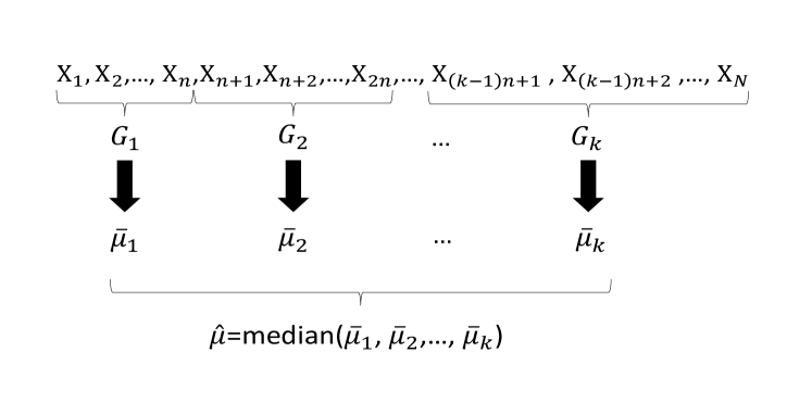
Figure 1: Feasibility of NP-EO oracle. The downward curve represents the critical values $c_{a}$ and $c_{b}$ in the classifier (5) such that the probability of type I error is $\alpha$, whereas the upward curve depicts the classifiers satisfying $R_{1}^{a}-R_{1}^{b}=\varepsilon$. The intersection of these two curves gives the critical values for the NP-EO classifier.

The existence of such a pair in one scenario is illustrated by Figure 1, where we assume that $R^{a}_{1}-R^{b}_{1}>\varepsilon$ for the NP oracle. More general discussion can be found in the proof of Theorem 1. In Figure 1, the vertical and horizontal axes are $c_{a}$ and $c_{b}$, representing respectively the $S=a$ and $S=b$ part of the thresholds in the classifier in (5). Thus, every point in the first quadrant represents such a classifier. In this figure, $c_{b}^{\prime}$ is the constant such that its corresponding $R_{1}^{b}=1-\varepsilon$. The solid downward curve represents pairs $(c_{a},c_{b})$ such that $R_{0}=\alpha$; note that

$$R_{0}(\phi^{\#}_{c_{a},c_{b}})=(1-F_{0,a}(c_{a}))\cdot p_{a|0}+(1-F_{0,b}(c_{b}))\cdot p_{b|0}\,,$$

so when $R_{0}$ is fixed at $\alpha$, $c_{a}$ is non-increasing as $c_{b}$ increases, which is shown in Figure 1. At the same time, the solid upward curve represents the threshold pairs $(c_{a},c_{b})$ such that $R_{1}^{a}-R_{1}^{b}=\varepsilon$. Since $R_{1}^{a}(\phi^{\#}_{c_{a},c_{b}})-R_{1}^{b}(\phi^{\#}_{c_{a},c_{b}})=F_{1,a}(c_{a})-F_{1,b}(c_{b}),$ so when $R_{1}^{a}-R_{1}^{b}$ is fixed at $\varepsilon$, $c_{a}$ is non-decreasing when $c_{b}$ increases, and hence the curve should be upward. As indicated in Figure 1, it can be shown that there must be an intersection of the two curves, which satisfies both the NP and EO constraints. Then, the generalized Neyman-Pearson lemma implies that the intersection must be an NP-EO oracle classifier.

Now we rationalize results in Theorem 1 on an intuitive level. Theorem 1 states that an NP-EO oracle can be formed by two separate parts, namely, $S=a$ component and $S=b$ component. This is understandable because, as long as a classifier $\phi$ takes into consideration the protected attribute $S$, it can always be rewritten as a two-part form, i.e., $\phi(X,S)=\phi^{a}(X)\cdot{\rm 1}\kern-2.40005pt{\rm I}\{S=a\}+\phi^{b}(X)\cdot{\rm 1}\kern-2.40005pt{\rm I}\{S=b\},$ where $\phi^{a}(\cdot)=\phi(\cdot,a)$ and $\phi^{b}(\cdot)=\phi(\cdot,b)$. Then, given the two-part form, it is not surprising that the best $\phi^{a}$ and $\phi^{b}$, in terms of group-wise type II error performance for a type I error level, adopt density ratios as scoring functions. Thus, as long as the two thresholds are adjusted so that NP and EO constraints are satisfied, the classifier in the form of equation (5) will have smaller $R_{1}^{a}$ and $R_{1}^{b}$ than other feasible classifiers and thus a smaller $R_{1}$.

We now present a simple example to illustrate the NP-EO oracle.

Example 1

Let $X^{0,a},X^{1,a},X^{0,b}$ and $X^{1,b}$ be $\mathcal{N}(0,1),\mathcal{N}(4,1),\mathcal{N}(0,9)$ and $\mathcal{N}(4,9)$ distributed random variables, respectively, and set ${\rm I}\kern-1.79993pt{\rm P}(S=a,Y=0)={\rm I}\kern-1.79993pt{\rm P}(S=a,Y=1)={\rm I}\kern-1.79993pt{\rm P}(S=b,Y=1)={\rm I}\kern-1.79993pt{\rm P}(S=b,Y=1)=0.25$. Then, the Bayes classifier is $\phi_{\text{Bayes}}={\rm 1}\kern-2.40005pt{\rm I}\{X>2\}$ and the NP oracle classifier for $\alpha=0.1$ is $\phi_{\text{NP}}={\rm 1}\kern-2.40005pt{\rm I}\{X>2.58\}$. If $\alpha=\varepsilon=0.1$, the NP-EO oracle classifier is $\phi_{\text{NP-EO}}={\rm 1}\kern-2.40005pt{\rm I}\{X>3.20\}{\rm 1}\kern-2.40005pt{\rm I}\{S=a\}+{\rm 1}\kern-2.40005pt{\rm I}\{X>2.53\}{\rm 1}\kern-2.40005pt{\rm I}\{S=b\}$. The graphical illustration of this example is depicted in Figure 2. We can calculate that $R_{0}(\phi_{\text{Bayes}})=0.137$, $R_{1}(\phi_{\text{Bayes}})=0.137$ and $L_{1}(\phi_{\text{Bayes}})=0.23$, violating both NP and EO constraints. The NP oracle, compared with the Bayes classifier, has a larger threshold. Consequently, $R_{0}(\phi_{\text{NP}})=0.1$, $R_{1}(\phi_{\text{NP}})=0.198$ and $L_{1}(\phi_{\text{NP}})=0.24$. The NP oracle classifier satisfies the NP constraint but violates the EO constraint. The NP-EO oracle classifier is more subtle. Its $S=a$ part threshold is larger than that of NP oracle classifier whereas the $S=b$ part threshold is slightly smaller, resulting in $R_{0}(\phi_{\text{NP-EO}})=0.100$, $R_{1}(\phi_{\text{NP-EO}})=0.262$ and $L_{1}(\phi_{\text{NP-EO}})=0.1$, so that the NP-EO oracle classifier satisfies both NP and EO constraints.

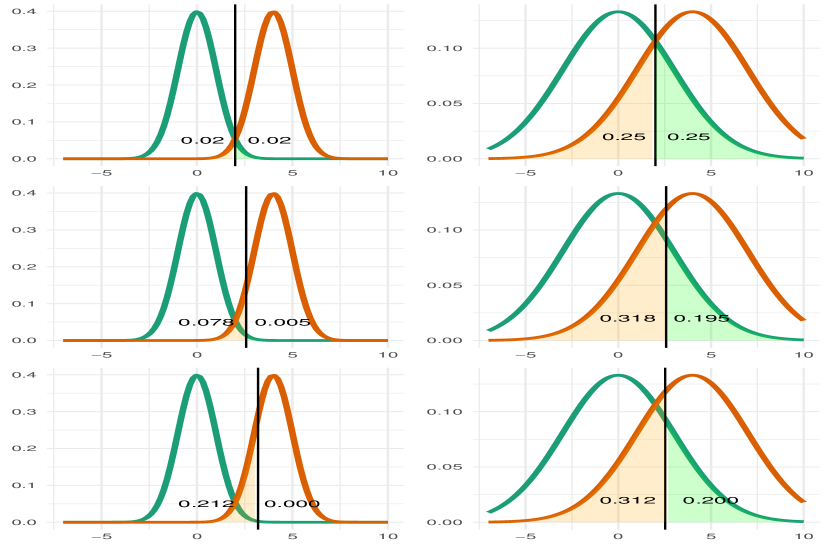
Figure 2: Plots of three classifiers in Example 1. The three rows, from top to bottom, represent figure illustration of the Bayes classifier, NP oracle classifier and NP-EO oracle classifier, respectively. The left panel illustrates the densities of $X^{0,a}$ and $X^{1,a}$ and the right panel those of $X^{0,b}$ and $X^{1,b}$. In every sub-figure, the green curve represents class $0$ density and the orange curve represents class $1$ density. In each row, the two thresholds of the classifier are indicated by the two black vertical lines. The type I and type II errors conditional on sensitive attribute are depicted respectively as the light green and light orange regions in every sub-figure with their values marked.

An NP-EO oracle classifier has a nice property: it is invariant to the changes in the proportions of class labels. This insight is concretized by the following proposition.

Proposition 1

Under conditions of Theorem 1, an NP-EO oracle classifier is invariant to the change in ${\rm I}\kern-1.79993pt{\rm P}(Y=0)$ (or equivalently ${\rm I}\kern-1.79993pt{\rm P}(Y=1)$), as long as the distributions of $X\mid(Y=y,S=s)$ (i.e., $X^{y,s}$) and $S\mid(Y=y)$ stay the same for each $y\in\{0,1\}$ and $s\in\{a,b\}$.

4 Methodology

In this section, we propose two sample-based NP-EO umbrella algorithms. Theorem 1 indicates that the density ratios are the best scores, with proper threshold choices. Hence plugging the density ratio estimates in equation (5) would lead to classifiers with good theoretical properties. In practice and more generally, however, practitioners can and might prefer to use scores from canonical classification methods (e.g., logistic regression and neural networks), which we also refer to as base algorithms. Inspired by (5), we construct classifiers of the generic form

$$\widehat{\phi}(X,S)={\rm 1}\kern-2.40005pt{\rm I}\{T^{a}(X)>c_{a}\}\cdot{\rm 1}\kern-2.40005pt{\rm I}\{S=a\}+{\rm 1}\kern-2.40005pt{\rm I}\{T^{b}(X)>c_{b}\}\cdot{\rm 1}\kern-2.40005pt{\rm I}\{S=b\}\,,$$ (6)

where $T^{a}(\cdot)$ and $T^{b}(\cdot)$ are given scoring functions for groups $S=a$ and $S=b$, respectively, and our task is to choose proper data-driven thresholds $c_{a}$ and $c_{b}$ that take into account the NP and EO constraints. This form is inspired by the NP-EO oracle classifier in the previous section by regarding $T^{a}$ and $T^{b}$ as the density ratios. We leave the more theory-oriented investigation on density ratio plug-ins for the future.

The classifier $\widehat{\phi}$ in (6) is trained on finite sample; thus it is random due to randomness of the sample, and the constraints in program (4) cannot be satisfied with probability $1$ in general. Therefore, we aim to achieve high-probability NP and EO constraints as follows,

$${\rm I}\kern-1.79993pt{\rm P}\left(R_{0}(\widehat{\phi})>\alpha\right)\leq\delta\,,$$ (7)

$${\rm I}\kern-1.79993pt{\rm P}\left(L_{1}(\widehat{\phi})>\varepsilon\right)\leq\gamma\,,$$ (8)

for pre-specified small $\delta,\gamma\in(0,1)$. Here, ${\rm I}\kern-1.79993pt{\rm P}$ is taken over the randomness of the training sample.

In Sections 4.1 and 4.2, we will present two umbrella algorithms: $\text{NP-EO}_{\text{OP}}$ and $\text{NP-EO}_{\text{MP}}$. The meaning of their names will become clear later. $\text{NP-EO}_{\text{OP}}$ is simpler and computationally lighter than $\text{NP-EO}_{\text{MP}}$. It is also “safer” in the sense that it achieves at least $1-\delta$ probability type I error control whereas $\text{NP-EO}_{\text{MP}}$ is only theoretically guaranteed to achieve at least $1-\delta^{+}$ probability control for some $\delta^{+}\searrow\delta$ as sample size grows. However, $\text{NP-EO}_{\text{OP}}$ sacrifices the power. In contrast, $\text{NP-EO}_{\text{MP}}$ achieves smaller type II error and does not violate exact high-probability NP constraint in numerical analysis, as demonstrated in Section 5. Moreover, $\text{NP-EO}_{\text{MP}}$ is a generalization of $\text{NP-EO}_{\text{OP}}$ in terms of threshold selection. Thus, it is convenient for readers to encounter $\text{NP-EO}_{\text{OP}}$ first.

4.1 The $\text{NP-EO}_{\text{OP}}$ umbrella algorithm

We now construct an algorithm that respects (7) and (8), and achieves type II error as small as possible. Denote by $\mathcal{S}^{y,s}$ the set of $X$ feature observations whose labels are $y$ and sensitive attributes are $s$, where $y\in\{0,1\}$ and $s\in\{a,b\}$. We assume that all the $\mathcal{S}^{y,s}$’s are independent, and instances within each $\mathcal{S}^{y,s}$ are i.i.d. Each $\mathcal{S}^{y,s}$ is divided into two halves: $\mathcal{S}^{y,s}_{\text{train}}$ for training scoring functions, and $\mathcal{S}^{y,s}_{\text{left-out}}$ for estimating the thresholds in the classifier (6).

First, all $\mathcal{S}^{y,s}_{\text{train}}$’s are combined together to train a scoring function (e.g., sigmoid function in logistic regression) $T:\mathcal{X}\times\{a,b\}\mapsto{\rm I}\kern-1.79993pt{\rm R}$; then we take $T^{a}(\cdot)=T(\cdot,a)$ and $T^{b}(\cdot)=T(\cdot,b)$. To determine $c_{a}$ and $c_{b}$, we select pivots to fulfill the NP constraint first and then adjust them for the EO constraint. A prior result leveraged to achieve the high-probability NP constraint is the NP umbrella algorithm developed by Tong et al., (2018). This algorithm adapts to all scoring-type classification methods (e.g., logistic regression and neural-nets), which we now describe. For an arbitrary (random) scoring function $S:\mathcal{X}\mapsto{\rm I}\kern-1.79993pt{\rm R}$ and i.i.d. class $0$ observations $\{X_{1}^{0},X_{2}^{0},\cdots,X_{n}^{0}\}$, a classifier that controls type I error under $\alpha$ with probability at least $1-\delta$ and achieves small type II error can be built as ${\rm 1}\kern-2.40005pt{\rm I}\{S(X)>s_{(k^{*})}\},$ where $s_{(k^{*})}$ is the $(k^{*})^{\text{th}}$ order statistic of $\{s_{1},s_{2},\cdots,s_{n}\}:=\{S(X_{1}^{0}),S(X_{2}^{0}),\cdots,S(X_{n}^{0})\}$ and $k^{*}$ is the smallest $k\in\{1,2,\cdots,n\}$ such that $\sum_{j=k}^{n}{n\choose j}(1-\alpha)^{j}\alpha^{n-j}\leq\delta.$ The smallest such $k$ is chosen to achieve the smallest type II error. The only condition for this high-probability type I error control is $n\geq\lceil\log\delta/\log(1-\alpha)\rceil$, a mild sample size requirement. More details of this algorithm are recollected from Tong et al., (2018) and provided in Appendix A.1.

Motivated by the NP umbrella algorithm, we apply $T^{s}(\cdot)$ to each instance in $\mathcal{S}^{y,s}_{\text{left-out}}$ to obtain $\mathcal{T}^{y,s}=\{t^{y,s}_{1},t^{y,s}_{2},\cdots,t^{y,s}_{n^{y}_{s}}\}$, where $n^{y}_{s}=|\mathcal{S}^{y,s}_{\text{left-out}}|$, $y\in\{0,1\}$, and $s\in\{a,b\}$. A natural starting point is to apply the NP umbrella algorithm (Tong et al.,, 2018) to the data with sensitive attributes $a$ and $b$ separately so that they both satisfy the NP constraint (7). Concretely, from the sorted set $\mathcal{T}^{0,a}=\{t^{0,a}_{(1)},t^{0,a}_{(2)},\cdots,t^{0,a}_{(n^{0}_{a})}\}$, the pivot $t^{0,a}_{(k^{0,a}_{*})}$ is selected as the $\left(k^{0,a}_{*}\right)^{\text{th}}$ order statistic in $\mathcal{T}^{0,a}$, where $k^{0,a}_{*}$ is the smallest $k\in\{1,\cdots,n^{0}_{a}\}$ such that $\sum_{j=k}^{n^{0}_{a}}{n^{0}_{a}\choose j}(1-\alpha)^{j}\alpha^{n_{a}^{0}-j}\leq\delta.$ The pivot $t^{0,b}_{(k^{0,b}_{*})}$ is selected similarly on $\mathcal{T}^{0,b}$. If $c_{a}\geq t^{0,a}_{(k^{0,a}_{*})}$ and $c_{b}\geq t^{0,b}_{(k^{0,b}_{*})}$, then the classifier $\widehat{\phi}$ in (6) satisfies

$${\rm I}\kern-1.79993pt{\rm P}\left(R_{0}^{a}(\widehat{\phi})>\alpha\right)\leq\delta\quad\text{ and }\quad{\rm I}\kern-1.79993pt{\rm P}\left(R_{0}^{b}(\widehat{\phi})>\alpha\right)\leq\delta\,,$$ (9)

by Proposition 1 in Tong et al., (2018). In view of (1), the above inequalities guarantee that the NP constraint can be achieved with probability at least $1-2\delta$. If we want to strictly enforce the $1-\delta$ probability type I error control in theory as in inequality (7), the $\delta$ parameter in our algorithm can be replaced by $\delta/2$.

The next step is to adjust the thresholds so that the resulting classifier also satisfies inequality (8), i.e., the high-probability EO constraint. To keep the NP constraint, we increase the values of thresholds for both groups. Similar to $\mathcal{T}^{0,a}$ and $\mathcal{T}^{0,b}$, we denote the sorted $\mathcal{T}^{1,s}=\{t^{1,s}_{(1)},t^{1,s}_{(2)},\cdots,t^{1,s}_{(n^{1}_{s})}\}$ for $s\in\{a,b\}$ and select $c_{a}$ from $\mathcal{T}^{1,a}$ and $c_{b}$ from $\mathcal{T}^{1,b}$ in order to facilitate the power calculation. Let

$$l_{a}=\sum_{j=1}^{n^{1}_{a}}{\rm 1}\kern-2.40005pt{\rm I}\left\{t^{1,a}_{j}\leq t^{0,a}_{(k^{0,a}_{*})}\right\}\quad\text{ and }\quad l_{b}=\sum_{j=1}^{n^{1}_{b}}{\rm 1}\kern-2.40005pt{\rm I}\left\{t^{1,b}_{j}\leq t^{0,b}_{(k^{0,b}_{*})}\right\}\,.$$ (10)

Then, $c_{a}$ is selected from $\{t^{1,a}_{(j)}:l_{a}<j\leq n^{1}_{a}\}$ and $c_{b}$ is selected from $\{t^{1,b}_{(j)}:l_{b}<j\leq n^{1}_{b}\}$ so that (9) holds. To this end, we investigate the distributions of

$$r^{a}_{1}(i)={\rm I}\kern-1.79993pt{\rm P}_{X^{1,a}}\left(T^{a}(X^{1,a})\leq t^{1,a}_{(i)}\right)\quad\text{ and }\quad r^{b}_{1}(j)={\rm I}\kern-1.79993pt{\rm P}_{X^{1,b}}\left(T^{b}(X^{1,b})\leq t^{1,b}_{(j)}\right)\,,$$

for $i>l_{a}$ and $j>l_{b}$. They are respectively the $S=a$ and $S=b$ components of the type II error of the classifier in (6), if we take $c_{a}=t^{1,a}_{(i)}$ and $c_{b}=t^{1,b}_{(j)}$; they are random because only the randomness of $X^{1,a}$ and $X^{1,b}$ are taken in ${\rm I}\kern-1.79993pt{\rm P}_{X^{1,a}}$ and ${\rm I}\kern-1.79993pt{\rm P}_{X^{1,b}}$. We need to understand these two quantities, so as to choosing from all eligible pairs $i$ and $j$ that satisfy the EO constraint.

The left hand side of the inequality in equation (8) can be written as ${\rm I}\kern-1.79993pt{\rm P}\left(\left|r^{a}_{1}(i)-r^{b}_{1}(j)\right|>\varepsilon\right),$ since we can consider the scoring function $T(\cdot)$ (and hence $T^{a}(\cdot)$ and $T^{b}(\cdot)$) as fixed due to independent pretraining of $T(\cdot)$. Since the random variables $r^{a}_{1}(i)$ and $r^{b}_{1}(j)$ are independent and admit similar definitions, we need only to study one of them as follows.

Let $X$ and $Y_{1},Y_{2},\cdots,Y_{n}$ be continuous, independent and identically distributed random variables. Moreover, let $c$ be a random variable that is independent of $X,Y_{1},\cdots,Y_{n}$ and define by $l=\sum_{j=1}^{n}{\rm 1}\kern-2.40005pt{\rm I}\{Y_{j}\leq c\}$. Our goal is to approximate the distribution of ${\rm I}\kern-1.79993pt{\rm P}_{X}(X\leq Y_{(k)})$ conditional on $l$ for $k>l$, which is needed for $r^{a}_{1}(i)$ and $r^{b}_{1}(j)$. Note that the conditional probability does not depend on the original distribution of $X$ and

$${\rm I}\kern-1.79993pt{\rm P}_{X}(X\leq Y_{(k)}\mid l)={\rm I}\kern-1.79993pt{\rm P}_{X}(X\leq Y_{(l)}\mid l)+{\rm I}\kern-1.79993pt{\rm P}_{X}(Y_{(l)}<X\leq Y_{(k)}\mid l)\,.$$

By using the property of the uniform order statistics, it can be shown that the above quantity has the same distribuion as $g_{c,l}+\left(1-g_{c,l}\right)B_{k-l,n-k+1}$ for $k>l$ with independent random variables $g_{c,l}={\rm I}\kern-1.79993pt{\rm P}(Y_{1}\leq c\mid l)$ and $B_{k-l,n-k+1}\sim\text{Beta}(k-l,n-k+1)$. It remains to approximate the distribution of $g_{c,l}$, which is $l/n$ if $c$ is a constant. Recall that $c$ is a random variable and $g_{c,l}=\mathbb{E}(F(c)|l)$ where $F$ is the cdf of $Y_{1}$. Writing $\theta=F(c)$, from the Bayesian point of view, the distribution of $g_{c,l}$ is the posterior distribution of $\theta$ given $n$ i.i.d. Bernoulli($\theta$) observations with sufficient statistic $l$. By Bernstein-von Mises theorem, $g_{c,l}$ is “close” to be normally distributed with mean $l/n$ (MLE in frequestist view) and variance equal to the Fisher information of the Bernoulli trial at MLE: $n^{-1}(l/n)(1-l/n)$.

The above discussion reveals that the distribution of $(r^{a}_{1}(i)\mid l_{a})$ can be approximated by $G^{1,a}+(1-G^{1,a})B_{i-l_{a},n^{1}_{a}-i+1}$ where $G^{1,a}\sim\mathcal{N}\left(\frac{l_{a}}{n^{1}_{a}},\frac{l_{a}/n^{1}_{a}(1-l_{a}/n^{1}_{a})}{n^{1}_{a}}\right).$ Similarly, the distribution of $(r_{1}^{b}(j)\mid l_{b})$ can be approximated. Let $F^{1,a}(i)$ and $F^{1,b}(j)$ be two independent random variables such that $F^{1,a}(i)=G^{1,a}+(1-G^{1,a})B_{i-l_{a},n^{1}_{a}-i+1},$ in distribution and $F^{1,b}(j)$ is defined analogously. Then, we can pick $(i,j)$ such that

$${\rm I}\kern-1.79993pt{\rm P}\left(\left|F^{1,a}(i)-F^{1,b}(j)\right|>\varepsilon\right)\leq\gamma\,.$$ (11)

Among these feasible pairs, the one that minimizes the empirical type II error, which can be calculated as $\left((i-1)+(j-1)\right)/(n_{a}^{1}+n_{b}^{1})$, should be selected; i.e., we select

$$(k^{*}_{a},k^{*}_{b})=\min_{\text{all feasible }(i,j)\text{ that satisfy}\eqref{eq:selection_criterion}}\frac{i+j-2}{n_{a}^{1}+n_{b}^{1}}\,.$$ (12)

The process to arrive at $(k^{*}_{a},k^{*}_{b})$ is illustrated in Figure 3. We propose an NP-EO classifier

$$\widehat{\phi}^{*}(X,S)={\rm 1}\kern-2.40005pt{\rm I}\{T^{a}(X)>t^{1,a}_{(k^{*}_{a})}\}\cdot{\rm 1}\kern-2.40005pt{\rm I}\{S=a\}+{\rm 1}\kern-2.40005pt{\rm I}\{T^{b}(X)>t^{1,b}_{(k^{*}_{b})}\}\cdot{\rm 1}\kern-2.40005pt{\rm I}\{S=b\}\,.$$

Note that, if none of $i\in\{l_{a}+1,\cdots,n^{1}_{a}\}$ and $j\in\{l_{b}+1,\cdots,n^{1}_{b}\}$ satisfy inequality (11), we say our algorithm does not provide a viable NP-EO classifier. This kind of exceptions have not occured in simulation or real data studies.

We summarize the above NP-EO umbrella algorithm in Algorithm 1. Note that in Step 8, the NP violation rate control at $\delta/2$ is needed for theoretical purpose (c.f. Theorem 2 and its proof). We will demonstrate through numerical analysis that it suffices to use $\delta$ instead. We also note that the steps to reach $(k^{*}_{a},k^{*}_{b})$ is summarized as the EO violation algorithm (Step 10) inside Algorithm 1, also presented separately as Algorithm 3 in the appendix for clarity. The next theorem provides a theoretical guarantee for $\widehat{\phi}^{*}(X,S)$.

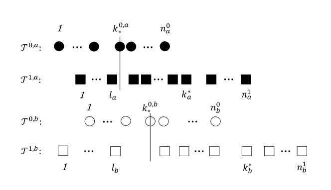
Figure 3: A cartoon illustration of the choices of $k_{a}^{*}$ and $k_{b}^{*}$. They are moved in the NP contrained feasible region (to the left) to search for the pairs that satisfy the EO constraint and to pick the most powerful pair. For every $\mathcal{T}^{y,s}$, the circles, or squares, in its corresponding row represent its sorted elements, ascending from left to right.

1

Input : $\mathcal{S}^{y,s}$: $X$ observations whose label $y\in\{0,1\}$ and sensitive attribute $s\in\{a,b\}$

$\alpha$: upper bound for type I error

$\delta$: type I error violation rate target

$\varepsilon$: upper bound for the type II error disparity

$\gamma$: type II error disparity violation rate target

2

3$\mathcal{S}^{y,s}_{\text{train}},\mathcal{S}^{y,s}_{\text{left-out}}\leftarrow$ random split on $\mathcal{S}^{y,s}$ for $y\in\{0,1\}$ and $s\in\{a,b\}$

4$\mathcal{S}_{\text{train}}\leftarrow\mathcal{S}^{0,a}_{\text{train}}\cup\mathcal{S}^{0,b}_{\text{train}}\cup\mathcal{S}^{1,a}_{\text{train}}\cup\mathcal{S}^{1,b}_{\text{train}}$

$T\leftarrow$ base classification algorithm$(\mathcal{S}_{\text{train}})$ ;

  // $T(\cdot,\cdot):\mathcal{X}\times\{a,b\}\mapsto{\rm I}\kern-1.79993pt{\rm R}$

5

6$T^{s}(\cdot)\leftarrow T(\cdot,s)$ for $s\in\{a,b\}$

7$\mathcal{T}^{y,s}\leftarrow T^{s}(\mathcal{S}^{y,s}_{\text{left-out}})$ for $y\in\{0,1\}$ and $s\in\{a,b\}$

8$n^{y}_{s}\leftarrow|\mathcal{T}^{y,s}|$ for $y\in\{0,1\}$ and $s\in\{a,b\}$

9$\mathcal{T}^{y,s}=\{t^{y,s}_{(1)},t^{y,s}_{(2)},\cdots,t^{y,s}_{(n^{y}_{s})}\}$ for $y\in\{0,1\}$ and $s\in\{a,b\}$

10$k^{0,s}_{*}\leftarrow\textsf{the NP umbrella algorithm}(n^{0}_{s},\alpha,\delta/2)$ for $s\in\{a,b\}$

11$l_{s}\leftarrow\max\{k\in\{1,2,\cdots,n_{s}^{1}\}:t^{1,s}_{(k)}\leq t^{0,s}_{(k^{0,s}_{*})}\}$ for $s\in\{a,b\}$

12$k^{*}_{a},k^{*}_{b}\leftarrow\textsf{EO violation algorithm}(l_{a},l_{b},n_{a}^{1},n_{b}^{1},\varepsilon,\gamma)$ in Appendix C.

Output : $\widehat{\phi}^{*}(X,S)={\rm 1}\kern-2.40005pt{\rm I}\{T^{a}(X)>t^{1,a}_{(k^{*}_{a})}\}\cdot{\rm 1}\kern-2.40005pt{\rm I}\{S=a\}+{\rm 1}\kern-2.40005pt{\rm I}\{T^{b}(X)>t^{1,b}_{(k^{*}_{b})}\}\cdot{\rm 1}\kern-2.40005pt{\rm I}\{S=b\}$

Algorithm 1 $\text{NP-EO}_{\text{OP}}$ umbrella algorithm [“OP” stands for One (pair of) Pivots]

Theorem 2

Let $\widehat{\phi}^{*}(\cdot,\cdot)$ be the classifier output by Algorithm 1 with parameters $(\alpha,\delta/2,\varepsilon,\gamma)$. Assume that the scoring function $T(\cdot,\cdot)$ is trained such that $T^{s}(X^{y,s})$ is a continuous random variable whose distribution function is strictly monotone for each $y\in\{0,1\}$ and $s\in\{a,b\}$, and that all distribution functions for $T^{s}(X^{y,s})$ have the same support. Furthermore, assume that $\min\{n^{0}_{a},n^{0}_{b}\}\geq\log(\delta/2)/\log(1-\alpha)$ Then it holds simultaneously that

$$\text{(a) }{\rm I}\kern-1.79993pt{\rm P}\left(R_{0}(\widehat{\phi}^{*})>\alpha\right)\leq\delta\quad\text{ and }\quad\text{(b) }{\rm I}\kern-1.79993pt{\rm P}\left(|R_{1}^{a}(\widehat{\phi}^{*})-R_{1}^{b}(\widehat{\phi}^{*})|>\varepsilon\right)\leq\gamma+\xi(n_{a}^{1},n_{b}^{1})\,,$$

in which $\xi(n^{1}_{a},n^{1}_{b})$ converges to $0$ as $n_{a}^{1}$ and $n_{b}^{1}$ diverge.

In Theorem 2, the conditions for distributions of $T^{s}(X^{y,s})$ ensure that the Bernstein-von Mises theorem can be invoked. Indeed, take the $S=a$ component for example, this theorem is applied to the class of binomial sample $l_{a}$ defined in equation (10), whose probability of success rate is ${\rm I}\kern-1.79993pt{\rm P}_{X^{1,a}}\left(T^{a}(X^{1,a})\leq t^{1,a}_{(i)}\right)$. The key issue here is that this random probability needs to be in the interior of $[0,1]$ with probability $1$, which is guaranteed by assumptions on $T^{s}(X^{y,s})$. Next, the assumptions for $n^{0}_{a}$ and $n^{0}_{b}$, adapted from Tong et al., (2018), are mild sample size requirements to ensure the high-probability NP constraint (c.f. part (a) of Theorem 2). We note that part (b) of Theorem 2 states that the type II error disparity violation rate can be controlled by $\gamma$ plus a term that vanishes asymptotically. This extra term, asymptotically negligible, is the price for the errors of Gaussian approximation on the distributions of $r_{1}^{a}$ and $r_{1}^{b}$.

4.2 The $\text{NP-EO}_{\text{MP}}$ umbrella algorithm

Algorithm 1 ($\text{NP-EO}_{\text{OP}}$) employs a “conservative” approach. Concretely, one pair of pivots, selected to ensure high-probability control on $R_{0}^{a}$ and $R_{0}^{b}$ simultaneously, serves as the lower bounds for the final thresholds. However, it could be suboptimal to control both $R_{0}^{a}$ and $R_{0}^{b}$, as our goal is to control $R_{0}$; indeed, it can induce unnecessarily small $R_{0}$, leading to large $R_{1}$ and hurting the power of the classifier. To amend this, we can start from a sensitive-attribute-agnostic NP classifier, and then adjust the thresholds for both groups while maintaining the overall type I error control. This gives us a wider class of pivots (than in the NP-EO${}_{\text{OP}}$ algorithm), and thus enables us to search for a more powerful classifier.

In our second and more general version of the NP-EO umbrella algorithm, we assume a slightly different sampling scheme for theoretical purpose. Denote by $\mathcal{S}^{y}$ the set of $(X,S)$ feature observations whose labels are $y$, where $y\in\{0,1\}$. We assume that $\mathcal{S}^{0}$ and $\mathcal{S}^{1}$ are independent and the instances within each $\mathcal{S}^{y}$ are i.i.d. Let $\mathcal{S}^{y,s}$ be the set of $X$ feature observations within $\mathcal{S}^{y}$ whose sensitive attribute is $s$, where $s\in\{a,b\}$. Under this sampling scheme, we assume that $n^{y}=|\mathcal{S}^{y}|$ is deterministic for $y\in\{0,1\}$. Denote by $n^{y}_{s}=|\mathcal{S}^{y,s}|$; then $n^{y}_{a}$ and $n^{y}_{b}$ are random, and $n^{y}=n^{y}_{a}+n^{y}_{b}$. Recall that we also denote $p_{s|y}={\rm I}\kern-1.79993pt{\rm P}(S=s\mid Y=y)$. Each $\mathcal{S}^{y,s}$ is split equally into $\mathcal{S}^{y,s}_{\text{train}}$ and $\mathcal{S}^{y,s}_{\text{left-out}}$. Training of scoring function $T$ (and thus $T^{a}$ and $T^{b}$) is the same as in Algorithm 1, and the scoring function $T$ is again applied to all elements in $\mathcal{S}^{y,s}_{\text{left-out}}$ to obtain the set of scores, $\mathcal{T}^{y,s}$, where $y\in\{0,1\}$ and $s\in\{a,b\}$. Similar to the approach outlined in Section 4.1, we first address the NP constraint. However, instead of two sensitive-attribute-specific thresholds, we start with an intermediate classifier that has the same threshold for both groups:

$$\widehat{\phi}_{*}(X,S) ={\rm 1}\kern-2.40005pt{\rm I}\{T(X,S)>t^{0}_{(k_{*})}\}$$

$$={\rm 1}\kern-2.40005pt{\rm I}\{T^{a}(X)>t^{0}_{(k_{*})}\}{\rm 1}\kern-2.40005pt{\rm I}\{S=a\}+{\rm 1}\kern-2.40005pt{\rm I}\{T^{b}(X)>t^{0}_{(k_{*})}\}{\rm 1}\kern-2.40005pt{\rm I}\{S=b\}\,,$$ (13)

where $t^{0}_{(k_{*})}$ is the $(k_{*})^{\text{th}}$ order statistic in $\mathcal{T}^{0}=\mathcal{T}^{0,a}\cup\mathcal{T}^{0,b}$ and $k_{*}$ is selected by the NP umbrella algorithm on $\mathcal{T}^{0}$. This threshold selection guarantees that $R_{0}(\widehat{\phi}_{*})$ is controlled under $\alpha$ with high probability. We will use $\widehat{\phi}_{*}$ as a bridge. Concretely, if a classifier of the form in (6) admits the same empirical type I error on $\mathcal{T}^{0}$ as $\widehat{\phi}_{*}$, their population-level type I errors should be close, and thus they can be both controlled under $\alpha$ with probability close to $1-\alpha$. One can see that $\widehat{\phi}_{*}$ makes $k^{0}_{a}+k^{0}_{b}$ correct classifications on $\mathcal{T}^{0}$, where

$$k^{0}_{a}=\sum_{j=1}^{n^{0}_{a}}{\rm 1}\kern-2.40005pt{\rm I}\{t^{0,a}_{j}\leq t^{0}_{(k_{*})}\}\quad\text{and}\quad k^{0}_{b}=\sum_{j=1}^{n^{0}_{b}}{\rm 1}\kern-2.40005pt{\rm I}\{t^{0,b}_{j}\leq t^{0}_{(k_{*})}\}\,.$$ (14)

In fact, if any $t^{0,a}_{(k_{a})}\in\mathcal{T}_{0,a}$ and $t^{0,b}_{(k_{b})}\in\mathcal{T}_{0,b}$, where $k_{a}\in[n^{0}_{a}]$ and $k_{b}\in[n^{0}_{b}]$, are chosen as the thresholds for $T^{a}$ and $T^{b}$ respectively, then as long as $k_{a}+k_{b}=k^{0}_{a}+k^{0}_{b}$, a classifier would have the same empirical type I error on $\mathcal{T}^{0}$ as $\widehat{\phi}_{*}$. Thus, to respect the high-probability NP constraint, we might choose any pair of thresholds $c_{a},c_{b}$ such that $c_{a}\geq t^{0,a}_{(k_{a})}$ and $c_{b}\geq t^{0,b}_{(k_{b})}$, where the pivots $t^{0,a}_{(k_{a})}$ and $t^{0,b}_{(k_{b})}$ satisfy $k_{a}+k_{b}=k^{0}_{a}+k^{0}_{b}$. This larger collection of pivot pairs makes power improvement possible.

The next goal is to satisfy the high-probability EO constraint. Here, the steps and reasoning are similar to Algorithm 1. Let $l_{a}(k_{a})$ and $l_{b}(k_{b})$, functions of $k_{a}$ and $k_{b}$, be defined analogously to (10), with $t^{0,a}_{(k^{0,a}_{*})}$ and $t^{0,b}_{(k^{0,b}_{*})}$ replaced by $t^{0,a}_{(k_{a})}$ and $t^{0,b}_{(k_{b})}$, respectively. Denote by $\ell_{a}=\{l_{a}(1),\cdots,l_{a}(n^{0}_{a})\}$, and $\ell_{b}=\{l_{b}(1),\cdots,l_{b}(n^{0}_{b})\}$. Similar to (10), as long as the two thresholds $c_{a},c_{b}$ are selected from $\left\{t^{1,a}_{(j)}:l_{a}(k_{a})+1<j\leq l_{a}(k_{a}+1)\right\}$ and $\left\{t^{1,b}_{(j)}:l_{b}(k_{b})+1<j\leq l_{b}(k_{b}+1)\right\}$, respectively, and $k_{a}+k_{b}=k_{a}^{0}+k_{b}^{0}$, the high probability NP constraint can be respected. Write

$${\rm I}\kern-1.79993pt{\rm P}\left(\left|r^{a}_{1}(i)-r^{b}_{1}(j)\right|>\varepsilon\right)={\rm I}\kern-1.79993pt{\rm E}_{s_{r},\ell_{a},\ell_{b}}{\rm I}\kern-1.79993pt{\rm P}\left(\left|r^{a}_{1}(i)-r^{b}_{1}(j)\right|>\varepsilon\mid s_{r},\ell_{a},\ell_{b}\right)\,.$$ (15)

In the above, $s_{r}$ stores the vector of the sensitive attributes associated with all instances in $\mathcal{S}^{y,s}_{\text{left-out}}$’s for $y\in\{0,1\}$ and $s\in\{a,b\}$. Recall that $r_{1}^{a}(i)$ and $r_{1}^{b}(j)$ are $R_{1}^{a}$ and $R_{1}^{b}$ if $t^{1,a}_{(i)}$ and $t^{1,b}_{(j)}$ are selected as thresholds. The next step is to approximate the conditional distributions of $r^{a}_{1}(i)$ and $r^{b}_{1}(j)$.

The arguments here are similar to the ones in Section 4.1 and we will start from a similar motivating example. Let $X$ and $Y_{1},Y_{2},\cdots,Y_{n}$ be continuous, independent, and identically distributed random variables. Now, let $c_{1},c_{2},\cdots,c_{m}$ be i.i.d. random variables that are independent of $X,Y_{1},\cdots,Y_{n}$ and define $l_{i}=\sum_{j=1}^{n}{\rm 1}\kern-2.40005pt{\rm I}\{Y_{j}\leq c_{i}\}$ for $i\in[m]$ and $\ell=\{l_{1},\cdots,l_{m}\}$. We will approximate the distribution of ${\rm I}\kern-1.79993pt{\rm P}_{X}(X\leq Y_{(k)})$ conditional on $\ell$, which equals

$${\rm I}\kern-1.79993pt{\rm P}_{X}(X\leq Y_{(k)})\mid\ell\overset{d}{=}\begin{cases}B_{k,l_{(1)}-k+1}G_{c,\ell}^{(1)},&k\leq l_{(1)}\,,\\ G_{c,\ell}^{(p)}+(G_{c,\ell}^{(p+1)}-G_{c,\ell}^{(p)})B_{k-l_{(p)},l_{(p+1)}-k+1},&l_{(p)}<k\leq l_{(p+1)},p\in[m-1]\,,\\ G_{c,\ell}^{(m)}+(1-G_{c,\ell}^{(m)})B_{k-l_{(m)},n-k+1}\,,&k>l_{(m)}\,,\end{cases}$$

where $\overset{d}{=}$ means “equal in distribution”, $B_{p,q}\sim Beta(p,q)$ and

$$G_{c,\ell}:=\left[G^{(1)}_{c,\ell},G^{(2)}_{c,\ell},\cdots,G^{(m)}_{c,\ell}\right]^{\top}:=[{\rm I}\kern-1.79993pt{\rm P}_{Y_{1}}(Y_{1}\leq c_{(1)}),{\rm I}\kern-1.79993pt{\rm P}_{Y_{1}}(Y_{1}\leq c_{(2)}),\cdots,{\rm I}\kern-1.79993pt{\rm P}_{Y_{1}}(Y_{1}\leq c_{(m)})]^{\top}\mid\ell\,.$$

Here, $G_{c,\ell}$ and the Beta random variables are independent. The next step is to approximate the distribution of $G_{c,\ell}$. With a slight abuse of notation, denote $c_{(0)}=-\infty,c_{(m+1)}=+\infty$ and $l_{(0)}=0,l_{(m+1)}=n$. It suffices to consider the joint distribution of the quantity

$$\Delta G_{c}\mid\Delta\ell:=[{\rm I}\kern-1.79993pt{\rm P}_{Y_{1}}\left(c_{(j-1)}<Y_{1}\leq c_{(j)}\right),j\in[m+1]]^{\top}\mid[l_{(i)}-l_{(i-1)},i\in[m]]^{\top}\,.$$

For fixed $c_{j}$, $\Delta G_{c}=[{\rm I}\kern-1.79993pt{\rm P}_{Y_{1}}\left(c_{(j-1)}<Y_{1}\leq c_{(j)}\right),j\in[m+1]]^{\top}$ can be viewed as the vector of probabilities for a multinomial distribution, and $\Delta\ell=[l_{(i)}-l_{(i-1)},i\in[m+1]]^{\top}$ is a multinomial random variable of size $n$ generated from this distribution. Then, the maximum likelihood estimator for $\Delta G_{c}$ is $\frac{\Delta\ell}{n}$. Therefore, when $c_{j}$ is random for $j\in[m]$, the distribution of $\Delta G_{c}\mid\Delta\ell$ is the posterior distribution of $\Delta G_{c}$ given $\Delta\ell$, and thus, by invoking Bernstein-von Mises theorem again, is “close to” Gaussian centered at $\frac{\Delta\ell}{n}$ with covariance matrix $\Sigma$ where

$$\Sigma_{i,j}=\begin{cases}\frac{1}{n}{\rm I}\kern-1.79993pt{\rm P}_{Y_{1}}\left(c_{(j-1)}<Y_{1}\leq c_{(j)}\right)\left(1-{\rm I}\kern-1.79993pt{\rm P}_{Y_{1}}\left(c_{(j-1)}<Y_{1}\leq c_{(j)}\right)\right),&i=j\,,\\ -\frac{1}{n}{\rm I}\kern-1.79993pt{\rm P}_{Y_{1}}\left(c_{(i-1)}<Y_{1}\leq c_{(i)}\right){\rm I}\kern-1.79993pt{\rm P}_{Y_{1}}\left(c_{(j-1)}<Y_{1}\leq c_{(j)}\right),&i\neq j\,.\end{cases}$$

Furthermore, we can use $(l_{(j)}-l_{(j-1)})/n$ to replace ${\rm I}\kern-1.79993pt{\rm P}_{Y_{1}}\left(c_{(j-1)}<Y_{1}\leq c_{(j)}\right)$ and obtain an estimated covariance matrix $\widehat{\Sigma}$. Thus, the estimation of ${\rm I}\kern-1.79993pt{\rm P}_{X}(X\leq Y_{(k)})\mid\ell$ is finished.

Despite being lengthy, it is actually straightforward to relate this example with the problem in this section. Recall that in view of (15), the goal is to approximate the distribution of $(r_{1}^{a}(i)\mid\ell_{a})$. Note that conditional on scoring function $T^{a}$ and $s_{r}$, the scores $t^{1,a},t^{1,a}_{1},t^{1,a}_{2},\cdots,t^{1,a}_{n^{1}_{a}}$ are i.i.d. random variables, and $t^{0,a}_{1},t^{0,a}_{2},\cdots,t^{0,a}_{n^{0}_{a}}$ are also i.i.d. random variables. Furthermore, the two groups of random variables are mutually independent. Moreover, $r_{1}^{a}(i)={\rm I}\kern-1.79993pt{\rm P}_{t^{1,a}}\left(t^{1,a}\leq t^{1,a}_{(i)}\right)$ and $l_{a}(j)=\sum_{h=1}^{n^{1}_{a}}{\rm 1}\kern-2.40005pt{\rm I}\{t^{1,a}_{h}\leq t^{0,a}_{(j)}\}$ for every $i\in[n^{1}_{a}]$ and $j\in[n^{0}_{a}]$. Therefore, the problem setting is in line with the previous motivating example, and thus, the distribution of $r_{1}^{a}(i)\mid\ell_{a}$ can be approximated in the same way. And the same procedure can be applied to the $S=b$ component. To conclude, we select $i$ and $j$ such that

$${\rm I}\kern-1.79993pt{\rm P}\left(\left\lvert\tilde{F}^{1,a}(i)-\tilde{F}^{1,b}(j)\right\rvert>\varepsilon\right)\leq\gamma\,,$$ (16)

where

$$\tilde{F}^{1,a}(i)\overset{d}{=}\begin{cases}B_{k,l_{a}(1)-k+1}\tilde{G}^{1,a}_{1},&k\leq l_{a}(1)\,,\\ \tilde{G}^{1,a}_{p}+\left(\tilde{G}^{1,a}_{p+1}-\tilde{G}^{1,a}_{p}\right)B_{k-l_{a}(p),l_{a}(p+1)-k+1},&l_{a}(p)<k\leq l_{a}(p+1),p\in[n^{0}_{a}-1]\,,\\ \tilde{G}^{1,a}_{n^{0}_{a}}+(1-\tilde{G}^{1,a}_{n^{0}_{a}})B_{k-l_{a}(n^{0}_{a}),n^{1}_{a}-k+1},&k>l_{a}(n^{0}_{a})\,,\end{cases}$$

and $\tilde{G}^{1,a}=\left[G^{1,a}_{1},\cdots,G^{1,a}_{n^{0}_{a}}\right]^{\top}$ is a Gaussian vector with mean $[l_{a}(1)/n^{1}_{a},\ldots,l_{a}(n^{0}_{a})/n^{1}_{a}]^{\top}$ and covariance matrix

$$\begin{bmatrix}\frac{(d_{a}(1)/n^{1}_{a})(1-d_{a}(1)/n^{1}_{a})}{n^{1}_{a}}&-\frac{(d_{a}(1)/n^{1}_{a})(d_{a}(2)/n^{1}_{a})}{n^{1}_{a}}&\cdots&-\frac{(d_{a}(1)/n^{1}_{a})(d_{a}(n^{0}_{a}+1)/n^{1}_{a})}{n^{1}_{a}}\\ -\frac{(d_{a}(2)/n^{1}_{a})(d_{a}(1)/n^{1}_{a})}{n^{1}_{a}}&\frac{(d_{a}(2)/n^{1}_{a})(1-d_{a}(2)/n^{1}_{a})}{n^{1}_{a}}&\cdots&-\frac{(d_{a}(2)/n^{1}_{a})(d_{a}(n^{0}_{a}+1)/n^{1}_{a})}{n^{1}_{a}}\\ \vdots&\vdots&\ddots&\vdots\\ -\frac{(d_{a}(n^{1}_{a}+1)/n^{1}_{a})(d_{a}(1)/n^{1}_{a})}{n^{1}_{a}}&-\frac{(d_{a}(n^{1}_{a}+1)/n^{1}_{a})(d_{a}(2)/n^{1}_{a})}{n^{1}_{a}}&\cdots&\frac{(d_{a}(n^{0}_{a}+1)/n^{1}_{a})(1-d_{a}(n^{0}_{a}+1)/n^{1}_{a})}{n^{1}_{a}}\end{bmatrix}\,.$$

Here,

$$d_{a}(k)=\begin{cases}l_{a}(1),&k=1\,,\\ l_{a}(k+1)-l_{a}(k),&k=2,3,\cdots,n^{0}_{a}-1\,,\\ n^{1}_{a}-l_{a}(n^{0}_{a}),&k=n^{0}_{a}\,.\end{cases}$$

Moreover, $\tilde{F}^{1,b}(j)$ is defined analogously. Details of this approximation can be found in Algorithm 4 in the Appendix. Next, one pair of $i$ and $j$ needs to be selected among all possible pairs satisfying (16). In Algorithm 1, we traverse all feasible pairs of $i$ and $j$ and choose one that minimizes the empirical type II error. It was computationally feasible because only $i,j$ such that $t^{1,a}_{(i)}>t^{0,a}_{(k^{0,a}_{*})}$ and $t^{1,b}_{(j)}>t^{0,b}_{(k^{0,b}_{*})}$ were considered. However, our generalized algorithm $\text{NP-EO}_{\text{MP}}$ has multiple pairs of pivots and it could be time-consuming to do the same. Therefore, we adopt the following heuristics:

1. Compute $t^{0}_{(k_{*})}$ by the NP umbrella algorithm. Then, select $k^{0}_{a}$ and $k^{0}_{b}$ by (14) and set $k_{a}=k^{0}_{a}$ and $k_{b}=k^{0}_{b}$.

2. Given $k_{a}$ and $k_{b}$, set $i=l_{a}(k_{a})+1$ and $j=l_{b}(k_{b})+1$, i.e., $i$ is such that $t^{1,a}_{(i)}$ is the smallest element in $\mathcal{T}^{1,a}$ larger than $t^{0,a}_{(k_{a})}$, and $j$ is selected analogously.

3. Apply Algorithm 4 to $i,j$ to calculate the approximate one-sided EO violation rates ${\rm I}\kern-1.79993pt{\rm P}(\tilde{F}^{1,a}(i)-\tilde{F}^{1,b}(j)\geq\varepsilon)$ and ${\rm I}\kern-1.79993pt{\rm P}(\tilde{F}^{1,b}(j)-\tilde{F}^{1,a}(i)\geq\varepsilon)$. If the former approximation is larger than $\gamma$, i.e., $\tilde{F}^{1,a}(i)$ is too large, increase $k_{b}$ by $1$ and decrease $k_{a}$ by $1$. If the latter approximation is larger than $\gamma$, increase $k_{a}$ by $1$ and decrease $k_{b}$ by $1$.

4. Repeat Steps (2) - (3) until the approximate value ${\rm I}\kern-1.79993pt{\rm P}(|\tilde{F}^{1,a}(i)-\tilde{F}^{1,b}(j)|\geq\varepsilon)$ is smaller than or equal to $\gamma$, then use $t^{1,a}_{(i)}$ and $t^{1,b}_{(j)}$ as thresholds.

Let us briefly discuss the above procedure. After key quantities $t^{0}_{(k_{*})},k^{0}_{a}$, and $k^{0}_{b}$ are determined, $k_{a}$ and $k_{b}$ are set to $k_{a}^{0}$ and $k_{b}^{0}$, respectively, in Step (1). In Step (2) and (3), an iterative method is used to find $i$ and $j$ that satisfy (16). For a pair of $k_{a}$ and $k_{b}$, we only look at $i$ and $j$ such that $t^{1,a}_{(i)}$ and $t^{1,b}_{(j)}$ are the smallest elements in $\mathcal{T}^{1,a}$ and $\mathcal{T}^{1,b}$ that are larger than $t^{0,a}_{(k_{a})}$ and $t^{0,b}_{(k_{b})}$, respectively. If this pair of $i$ and $j$ fails to satisfy (16), we adjust $k_{a}$ and $k_{b}$, and then update $i$ and $j$ accordingly. For example, if ${\rm I}\kern-1.79993pt{\rm P}(\tilde{F}^{1,a}(i)-\tilde{F}^{1,b}(j)\geq\varepsilon)>\gamma$, i.e., $\tilde{F}^{1,a}(i)$ is too large and $\tilde{F}^{1,b}(j)$ is too small, we decrease $k_{a}$ by $1$ and increase $k_{b}$ by $1$, so that $k_{a}+k_{b}=k_{a}^{0}+k_{b}^{0}$ and thus high-probability NP constraint is respected. After $k_{a}$ and $k_{b}$ are updated, $i$ and $j$ are selected in the same way described above. This updating procedure can be done iteratively until (16) is reached. Then, the scores $t^{1,a}_{(i)}$ and $t^{1,b}_{(j)}$ are selected as the thresholds of the resulting classifier.

1

Input : $\mathcal{S}^{y,s}$: $X$ observations whose label $y\in\{0,1\}$ and sensitive attribute $s\in\{a,b\}$

$\alpha$: upper bound for type I error

$\delta$: type I error violation rate target

$\varepsilon$: upper bound for the type II error disparity

$\gamma$: type II error disparity violation rate target

2

3$\mathcal{S}^{y,s}_{\text{train}},\mathcal{S}^{y,s}_{\text{left-out}}\leftarrow$ random split on $\mathcal{S}^{y,s}$ for $y\in\{0,1\}$ and $s\in\{a,b\}$

4$\mathcal{S}_{\text{train}}\leftarrow\mathcal{S}^{0,a}_{\text{train}}\cup\mathcal{S}^{0,b}_{\text{train}}\cup\mathcal{S}^{1,a}_{\text{train}}\cup\mathcal{S}^{1,b}_{\text{train}}$

$T\leftarrow$ base classification algorithm$(\mathcal{S}_{\text{train}})$ ;

  // $T(\cdot,\cdot):\mathcal{X}\times\{a,b\}\mapsto{\rm I}\kern-1.79993pt{\rm R}$

5

6$T^{s}(\cdot)\leftarrow T(\cdot,s)$ for $s\in\{a,b\}$

7$\mathcal{T}^{y,s}\leftarrow T^{s}(\mathcal{S}^{y,s}_{\text{left-out}})$ for $y\in\{0,1\}$ and $s\in\{a,b\}$

8$n^{y}_{s}\leftarrow|\mathcal{T}^{y,s}|$ for $y\in\{0,1\}$ and $s\in\{a,b\}$

9$\mathcal{T}^{0}=\mathcal{T}^{0,a}\cup\mathcal{T}^{0,b}=\{t^{0}_{(1)},t^{0}_{(2)},\cdots,t^{0}_{(n^{0})}\}$, where $n^{0}=n^{0}_{a}+n^{0}_{b}$

10$\mathcal{T}^{y,s}=\{t^{y,s}_{(1)},t^{y,s}_{(2)},\cdots,t^{y,s}_{(n^{y}_{s})}\}$ for $y\in\{0,1\}$ and $s\in\{a,b\}$

11$k_{*}\leftarrow\textsf{the NP umbrella algorithm}(n^{0},\alpha,\delta)$

12$\{l_{s}(1),\cdots,l_{s}(n^{0}_{s})\}\leftarrow\left\{\sum_{j=1}^{n^{1}_{s}}{\rm 1}\kern-2.40005pt{\rm I}\{t^{1,s}_{j}\leq t^{1,s}_{(1)}\},\cdots,\sum_{j=1}^{n^{1}_{s}}{\rm 1}\kern-2.40005pt{\rm I}\{t^{1,s}_{j}\leq t^{1,s}_{(n^{1}_{s})}\}\right\}$ for $s\in\{a,b\}$

13$k_{s}\leftarrow k^{0}_{s}\leftarrow\sum_{j=1}^{n^{0}_{s}}{\rm 1}\kern-2.40005pt{\rm I}\{t^{0,s}_{j}\leq t^{0}_{(k_{*})}\}$ for $s\in\{a,b\}$

14$(k^{*}_{a},k^{*}_{b})\leftarrow\textbf{Order selection algorithm}(k_{s},n^{y}_{s},l_{s}(1),\cdots,l_{s}(n^{0}_{s}),\varepsilon,\gamma)$ for $s\in\{a,b\}$

Output : $\widehat{\phi}^{**}(X,S)={\rm 1}\kern-2.40005pt{\rm I}\{T^{a}(X)>t^{1,a}_{(k^{*}_{a})}\}\cdot{\rm 1}\kern-2.40005pt{\rm I}\{S=a\}+{\rm 1}\kern-2.40005pt{\rm I}\{T^{b}(X)>t^{1,b}_{(k^{*}_{b})}\}\cdot{\rm 1}\kern-2.40005pt{\rm I}\{S=b\}$

Algorithm 2 $\text{NP-EO}_{\text{MP}}$ umbrella algorithm [“MP” means Multiple (Pairs of) Pivots]

This more general version of NP-EO umbrella algorithm is summarized as Algorithm 2. Instead of using only one pair of pivots in Algorithm 1, Algorithm 2 uses multiple pairs. Concretely, the two pivots $t^{0,a}_{(k_{a})}$ and $t^{0,b}_{(k_{b})}$ can be increased or decreased based on their resulting one-sided type II error disparities. Algorithm 1 controls $R^{a}_{0}$ and $R^{b}_{0}$ simultaneously to achieve the high-probability NP constraint. Algorithm 2, however, relieves the control on one of them but uses the empirical type I errors as a bridge to have an “approximate control” on the population-level type I error. This increases the risk of failing the exact probability target of type I error control. However, the advantage of this less conservative approach is obvious: lowering the pivot on one side allows a higher classification power. Indeed, numerical evidence from Section 5.1 suggests that Algorithm 2 has a lower type II error compared to Algorithm 1 and a higher type I error. Furthermore, both algorithms satisfy high-probability NP and EO constraints. Same as in Section 4.1, in theory there could be exceptions that no $(i,j)$ satisfies (16). However, we have not met this exception in data analysis.

Now we are ready to present the theoretical guarantee for Algorithm 2. Since the empirical type I errors are used as a bridge to link the population-level type I errors for different pairs of pivots, a concentration of empirical type I errors towards population-level type I error is needed. Thus, in the following theoretical result, we allow an $\eta$-error between empirical and population-level type I errors. That is, the target probability for type I error control will be set at $\alpha-\eta$ where $\eta$ is a small number compared with $\alpha$. However, this is not needed in numerical implementation of Algorithm 2.

Theorem 3

Let $\widehat{\phi}^{**}(\cdot,\cdot)$ be the classifier output by Algorithm 2 with parameters $(\alpha-\eta,\delta,\varepsilon,\gamma)$ for $0<\eta\ll\alpha$. Assume that the scoring function $T(\cdot,\cdot)$ is trained such that the same conditions in Theorem 2 hold and that $n^{0}\geq\log(\delta)/\log(1-\alpha)$. Then it holds simultaneously that

$$(a)\quad{\rm I}\kern-1.79993pt{\rm P}\left(R_{0}(\widehat{\phi}^{**})>\alpha\right)\leq\delta+2e^{-\frac{1}{32}n^{0}(p_{a|0}-\eta/8)\eta^{2}}+2e^{-\frac{1}{32}n^{0}(p_{b|0}-\eta/8)\eta^{2}}+2e^{-\frac{1}{32}n^{0}\eta^{2}}+2e^{-\frac{1}{2}n^{0}\eta^{2}}\,,$$

$$(b)\quad{\rm I}\kern-1.79993pt{\rm P}\left(|R_{1}^{a}(\widehat{\phi}^{**})-R_{1}^{b}(\widehat{\phi}^{**})|>\varepsilon\right)\leq\gamma+\xi^{\prime}(n^{1})\,,$$

in which $\xi^{\prime}(n^{1})$ converges to $0$ as $n^{1}=n^{1}_{a}+n^{1}_{b}$ diverges.

The proof of this theorem is presented in the Appendix. Here, we remark that the main difference between Theorems 2 and 3 is in part (a). In Theorem 2, the type I error is controlled with probability at least $1-\delta$, whereas in Theorem 3, $\widehat{\phi}^{**}$ only gives an “approximately” $1-\delta$ type I error control. This is not surprising since we use empirical type I errors to estimate population-level type I error for $\widehat{\phi}^{**}$ and thus to make sure their population-level type I errors are close by matching the empirical type I errors. As such, the exponential terms in part (a) of Theorem 3 compensate for this estimation.

5 Numerical results

In this section, we present simulation and real-data evidence that supports the effectiveness of the newly proposed NP-EO algorithms. In each simulation setting, all trained algorithms are evaluated on a large test set to the approximate the (population-level) type I and type II errors. This procedure is repeated $1{,}000$ times and thus $1{,}000$ copies of (approximate) type I and type II errors can be acquired. Then, the NP violation rate is computed as the proportion of type I error exceeding the target level defined in the NP constraint. Similarly, the EO violation rate is computed as the proportion of type II error disparity exceeding the target level defined in the EO constraint. Finally, recall that for $\text{NP-EO}_{\text{OP}}$ algorithm, we use $\delta$, instead of $\delta/2$, in Algorithm (1).

5.1 Simulation

In all settings, for each $y\in\{0,1\}$ and $s\in\{a,b\}$, we generate $n^{y,s}$ training observations and $100n^{y,s}$ test observations. We compare the $\text{NP-EO}_{\text{OP}}$ and $\text{NP-EO}_{\text{MP}}$ algorithms with three existing algorithms, namely, the classical algorithm, NP umbrella algorithm, and NP umbrella algorithm mixed with random guesses. Here, the classical algorithm (e.g., logistic regression, support vector machines) is the base algorithm without any adjustment for either the NP or EO constraint. The NP umbrella algorithm adjusts base algorithms for the NP constraint and it is described in Section A.1.

The NP umbrella algorithm mixed with random guesses, inspired by Hardt et al., (2016), works as follows. We start with an NP classifier, $\widehat{\phi}_{\text{NP}}$, trained by the NP umbrella algorithm. Without loss of generality, we assume $R_{1}^{a}(\widehat{\phi}_{\text{NP}})>R_{1}^{b}(\widehat{\phi}_{\text{NP}})$. A naive method to make the EO constraint satisfied is to increase type II error for $S=b$ by adding noise via a random guess classifier $\phi_{\text{RG}}$ with ${\rm I}\kern-1.79993pt{\rm P}(\phi_{\text{RG}}=1)=\alpha$. Then, for an observation in the testing sample with $S=a$, we use $\widehat{\phi}_{\text{NP}}$ only; for an observation with $S=b$, with probability $p$, $\widehat{\phi}_{\text{NP}}$ is selected to classify this observation, and with probability $1-p$, $\phi_{\text{RG}}$ is used. Note that $R_{1}^{b}(\phi_{\text{RG}})=1-\alpha$. Then, for this mixed classifier $\widehat{\phi}_{\text{mixed}}$, $R_{1}^{a}(\widehat{\phi}_{\text{mixed}})=R_{1}^{a}(\widehat{\phi}_{\text{NP}})$ and $R_{1}^{b}(\widehat{\phi}_{\text{mixed}})=pR_{1}^{b}(\widehat{\phi}_{\text{NP}})+(1-p)(1-\alpha)$. As long as $\widehat{\phi}_{\text{NP}}$ is more powerful than $\phi_{\text{RG}}$ on group $a$, i.e., $R_{1}^{a}(\widehat{\phi}_{\text{NP}})\leq 1-\alpha$, $\widehat{\phi}_{\text{mixed}}$ can achieve equality of opportunity by choosing $p$ properly.

In this simulation, we choose the probability $p$ by $20$-fold cross validation: we train an NP classifier on $19$ folds of the training data and compute the estimated $R^{a}_{1}(\widehat{\phi}_{\text{NP}})$ and $R_{1}^{b}(\widehat{\phi}_{\text{NP}})$ on the left-out fold. Since $R^{a}_{1}(\phi_{\text{RG}})$ and $R_{1}^{b}(\phi_{\text{RG}})$ are explicit, we can directly estimate $R^{a}_{1}(\widehat{\phi}_{\text{mixed}})$, $R^{b}_{1}(\widehat{\phi}_{\text{mixed}})$ and thus type II error disparity for every value of $p$ and the option of adding random guesses for either $S=a$ or $S=b$. We traverse all the combinations of $p=0,0.1,0.2,0.3,\cdots,0.9$ and the options of adding random guesses to both $S$ components. Next, for every combination, we calculate the estimated type II error disparity for every fold and thus can estimate the estimated probability of type II error disparity exceeding $\varepsilon$. Finally, we select the the combination such that this estimated probability is smaller than or equal to $\gamma$. If there are multiple such combinations, we select the one with the largest $p$. Then the resulting $\widehat{\phi}_{\text{mixed}}$ satisfies high-probability NP and EO constraints.

Simulation 1

Let $X^{y,s}$ be multidimensional Gaussian distributed with mean $\mu_{y,s}$ and covariance matrix $\Sigma_{y,s}$ for each $y\in\{0,1\}$ and $s\in\{a,b\}$. Here, $\mu_{0,a}=(1,2,1)^{\top}$, $\mu_{1,a}=(0,0,0)^{\top}$, $\mu_{0,b}=(0,0,2)^{\top}$ and $\mu_{1,b}=(1,0,-1)^{\top}$. Moreover

$$\Sigma_{y,a}=\begin{pmatrix}2&-1&0\\ -1&2&-1\\ 0&-1&2\end{pmatrix}\quad\quad\text{and}\quad\quad\Sigma_{y,b}=\begin{pmatrix}1&0&0\\ 0&2&0\\ 0&0&1\end{pmatrix}\,,$$

for every $y\in\{0,1\}$. Furthermore, $n^{0,a}=800$, $n^{1,a}=400$, $n^{0,b}=1200$ and $n^{1,b}=1600$. We set $\alpha=0.05$, $\delta=0.05$, $\varepsilon=0.2$ and $\gamma=0.05$. The base algorithm used is logistic regression. The numerical results associated with this simulation are reported in Table 1.

Table 1: Averages of type I and II errors, along with violation rates of the NP and EO constraints over $1{,}000$ repetitions for Simulation 1. Standard error of the means ($\times 10^{-4}$) in parentheses

average of type I errors average of type II errors NP violation rate EO violation rate $\text{NP-EO}_{\text{OP}}$ $.012(1.13)$ $.480(12.75)$ $0(0)$ $.046(66.28)$ $\text{NP-EO}_{\text{MP}}$ $.039(1.92)$ $.387(14.74)$ $.033(56.52)$ $.029(53.09)$ NP mixed with random guess $.035(1.61)$ $.657(23.25)$ $.010(31.48)$ $.037(59.72)$ NP $.039(1.97)$ $.163(3.78)$ $.047(66.96)$ $1(0)$ classical $.094(1.79)$ $.096(1.35)$ $1(0)$ $1(0)$

Simulation 2

Let $X^{y,s}$ be uniformly distributed in a three dimensional ball $B_{y,s}$ with radius $1$ and centered at $O_{y,s}$, where $O_{0,a}=(0,0,0)^{\top}$, $O_{1,a}=(1,0,-1)^{\top}$, $O_{0,b}=(1,1,1)^{\top}$ and $O_{1,b}=(-1,1,0)^{\top}$. Furthermore, $n^{0,a}=800$, $n^{1,a}=400$, $n^{0,b}=1200$ and $n^{1,b}=1600$. We also set $\alpha=0.05$, $\delta=0.05$, $\varepsilon=0.2$ and $\gamma=0.05$. The base algorithm used is logistic regression. The numerical results associated with this simulation are reported in Table 2.

Table 2: Averages of type I and II errors, along with violation rates of NP and EO constraints over $1{,}000$ repetitions for Simulation 2. Standard error of the means ($\times 10^{-4}$) in parentheses

average of type I errors average of type II errors NP violation rate EO violation rate $\text{NP-EO}_{\text{OP}}$ $.012(1.12)$ $.478(12.67)$ $0(0)$ $.053(70.88)$ $\text{NP-EO}_{\text{MP}}$ $.038(2.01)$ $.346(14.11)$ $.030(53.97)$ $.070(80.72)$ NP mixed with random guess $.035(1.55)$ $.588(21.11)$ $.006(24.43)$ $.009(29.88)$ NP $.034(2.45)$ $.191(6.43)$ $.029(53.09)$ $1(0)$ classical $.094(1.88)$ $.094(1.39)$ $1(0)$ $1(0)$

In both simulations, the classical classifier admits the lowest type II error; the NP classifier comes in the second place. This is not surprising as the NP paradigm controls the type I error to a low level with high probability, thereby resulting in a higher type II error. The NP and EO violation rates are both higher than the target levels for the classical classifier, whereas the NP classifier fails to keep the EO violation rate under the target level. These two classifiers adopt no design for EO adjustments; thus, it is expected that the EO requirement would fail.

The remaining three algorithms, $\text{NP-EO}_{\text{OP}}$, $\text{NP-EO}_{\text{MP}}$ and NP mixed with random guesses, are built to achieve the high-probability NP and EO constraints. All three algorithms produce an overall type II error larger than that of the NP paradigm. This is the price paid for equality in our classification algorithms. For reference, we remark that the “nearly trivial” NP-EO classifier, a random guess that return $1$ with probability $0.05$ and $0$ otherwise, has an overall type II error as high as $0.95$. Benchmarked against this result, the classifiers listed in both Tables 1 and 2 have much smaller type II errors. Moreover, in terms of the overall type II error, it is clear that $\text{NP-EO}_{\text{OP}}$ and $\text{NP-EO}_{\text{MP}}$ outperform NP mixed with random guesses, suggesting the effectiveness of our proposed algorithms. Between the two proposed algorithms, $\text{NP-EO}_{\text{MP}}$ yields larger average overall type I error and type I error violation rate, and smaller overall type II error than $\text{NP-EO}_{\text{OP}}$, which agrees with the argument in Section 4.2 that $\text{NP-EO}_{\text{MP}}$ uses multiple pivots to select thresholds more effectively. In conclusion, the two simulation studies illustrate that our proposed algorithms under the NP-EO paradigm are able to achieve the goals of regulating equality of opportunities and controlling type I error while only paying a modest price in terms of the less consequential type II error.

5.2 Real data analysis

In many countries, lenders’ discrimination against a certain social group other than creditworthiness is either illegal or socially unacceptable. Most notably, the Equal Credit Opportunity Act in the US explicitly makes it unlawful for any creditor to discriminate against any applicant on the basis of race, color, sex, and other non-credit related social factors. Nevertheless, ample evidence shows that Hispanic and Black borrowers have less access to credits or pay a higher price for mortgage loans in the US (Munnell et al.,, 1996; Charles et al.,, 2008; Hanson et al.,, 2016; Bayer et al.,, 2018).

With the emergence of the FinTech market, statistical and machine learning techniques have gained increasing popularity in lending decisions by both traditional financial institutions and peer-to-peer lending and crowd-sourcing platforms. An important regulatory concern in this development is whether algorithmic decision-making promotes or impedes impermissible discrimination. Recently, Bartlett et al., (2022) show that algorithmic lending reduces rate disparities between Latinx/African-American borrowers and other borrowers in consumer-lending markets but cannot eliminate the bias. Fuster et al., (2022) find that, in the US mortgage market, Black and Hispanic borrowers are disproportionately less likely to gain from the introduction of machine learning in lending decisions. Central in the welfare judgement of algorithmic lending is the tradeoff between efficiency (controlling default risk) and equality (non-disparate treatment). In the section, we illustrate how our proposed algorithms can help address this question with an example of potential gender bias in credit card consumption in Taiwan.

We focus on this case for two reasons. First, gender discrimination is a significant phenomenon in credit lending markets worldwide. Alesina et al., (2013) find that Italian women pay more for overdraft facilities than men. Bellucci et al., (2010) and Andrés et al., (2021) show that female entrepreneurs face tighter credit availability in Italy and Spain. Ongena and Popov, (2016) document a strong correlation between gender bias and credit access across developing countries. Second, practically, the Taiwanese credit card dataset is simple, transparent, and has clear labelling of payment status that enables an analysis of financial risk.

The dataset is from Yeh and Lien, (2009), which has been widely used to evaluate various data mining techniques. This dataset depicts the given credit, demographic features, and payment history of $30{,}000$ individuals during April 2005 to September 2005. Importantly, it includes a binary status of the payment: either default, encoded by $0$, or non-default, encoded by $1$. Among all $30{,}000$ records, $6{,}636$ of them are labelled as $0$, i.e., default. In this dataset, a person is default if they fail to repay the credit card in October 2005. The payment status defines the type I/II errors in the classification problem, and the protected attribute is gender. In this dataset, $11{,}888$ people are labelled as male and $18{,}112$ are labelled as female. Fitting such a typical credit-lending problem into the NP-EO classification framework, banks primarily want to control the risk of misclassifying someone who will default as non-default (type I error) although they also want to minimize the chance of letting go non-defaulters (type II error). Furthermore, by regulation or as a social norm, fairness requires banks not to discriminate against qualified applicants on the basis of gender. Therefore, to obtain the dual goal of risk control and fairness, our classification problem needs to satisfy the NP constraint and the EO constraint. We also note that since we already illustrated in Section 5.1 that the NP classifier mixed with random guesses performs worse than our proposed algorithms in all simulation settings, we do not include this classifier in this real data section.

We use $1/3$ of the data for training and the other $2/3$ for test, with stratification in both protected attribute and label. As an illustrative example, we set $\alpha=0.1$, $\delta=0.1$, $\varepsilon=0.05$ and $\gamma=0.1$. The base algorithm used is random forest. The process is repeated 1000 times, and the numerical results are presented in Table 3. Using the classical classifier, the high-probability EO constraint is satisfied. Indeed, the EO violation rate in Table 3 is $0$, indicating that the random forest under the classic paradigm is “fair” and “equal” in terms of gender. This is not entirely surprising given that gender bias in modern Taiwan is not a significant concern. The problem with this classifier is that it produces a type I error of $0.633$, which is prohibitively high for nearly any financial institution. Benchmarked against the modest NP constraint ($\alpha=0.1$), the violation rate is $1$, imposing too much risk to the banks.

Table 3: (Averages of type I and II errors, along with violation rates of NP and EO constraints over 1,000 repetitions for credit card dataset. Standard error of the means ($\times 10^{-4}$) in parentheses

average of type I errors average of type II errors NP violation rate EO violation rate $\text{NP-EO}_{\text{OP}}$ $.081(3.11)$ $.720(6.65)$ $.033(56.52)$ $.034(57.34)$ $\text{NP-EO}_{\text{MP}}$ $.089(2.99)$ $.701(6.23)$ $.114(100.55)$ $.054(71.51)$ NP $.088(3.02)$ $.700(6.26)$ $.111(99.39)$ $.482(158.10)$ classical $.633(4.02)$ $.059(1.31)$ $1(0)$ $0(0)$

When the NP paradigm alone is employed, the EO violation rate surges to $0.482$, demonstrating a conflict between the banks’ private gain of improving risk control and the society’s loss of achieving fairness. When the $\text{NP-EO}_{\text{OP}}$ and $\text{NP-EO}_{\text{MP}}$ algorithms are employed, both the NP and EO constraints are satisfied with very small violation rates, and the classifiers simultaneously achieve the goals of risk control and fairness. The cost that the banks have to bear is missing some potential business opportunities from non-defaulters, which is reflected in the higher overall type II error committed by either NP-EO algorithm. Consistent with the simulation results in Section 5.1, compared to $\text{NP-EO}_{\text{OP}}$, $\text{NP-EO}_{\text{MP}}$ produces a smaller the overall type II error while maintaining satisfactory (yet larger) violation rates.

6 Discussion

This paper is motivated by two practical needs in algorithmic design: a private user’s need to internalize social consideration and a social planner’s need to facilitate private users’ compliance with regulation. The challenge in fulfilling these needs stems from the conflict between the private and social goals. Notably, the social planner’s promotion of fairness and equality may constrain private users’ pursuit of profits and efficiency. In an ideal world without measurement and sampling problems, such a private-public conflict can be best resolved by maximizing a social welfare function with well-defined private and public components. Statistical tools hardly play any role in this process. However, when knowledge about the social welfare function is partial, measurement of each component in the objective is imperfect, and consequences of predictive errors are uncertain, statistical innovation is called for to step into the endeavor of resolving the private-public conflict. Our work is a response to this challenge.

In a classification setting, we propose the NP-EO paradigm, in which we incorporate a social consideration into a constrained optimization problem with the less-important private goal (type II error) being the objective while the social goal (equal opportunity) and the more-important private goal (type I error) as constraints. Algorithmic decisions with such restrictions provide safeguards against deviations from the social goal and avoid significant damage to the private goal, leaving the private-social conflict mostly absorbed by the less-consequential private consideration. We believe that our approach can be applied to a wide range of settings beyond the problem we are handling in this paper.

We do not claim that our proposed NP-EO paradigm is superior to other classification paradigms. Rather, we are proposing an alternative framework to handle private-social conflicts in algorithmic design. Central in our analysis is a perspective of gaining security through statistical control when multiple objectives have to be compromised. Key to our methodological innovation is a principled way to redistribute specific errors so that the resulting classifiers have high-probability statistical guarantees.

Possible future research direction include but not limited to: (i) extending the solutions to multiple constraints with respects to the social norms, which can be multiple attributes such as race and gender or multiple levels such as race, (ii) working with parametric models, such as the linear discriminant analysis (LDA) model, to derive model-specific NP-EO classifiers that address small sample size problem and satisfy oracle type inequalities, (iii) replacing type I error constraint by other efficiency constraints, and replacing the EO constraint by other fairness criteria, and (iv) studying fairness under other asymmetric efficiency frameworks such as isotonic subgroup selection in Müller et al., (2023).

Appendix A Preliminaries

A.1 NP umbrella algorithm

The NP umbrella algorithm developed in Tong et al., (2018) adapts all scoring-type classification methods (e.g., logistic regression, random forest, neural nets) so that the resulting classifiers have the type I error bounded from above by a user-specified level $\alpha$ with pre-specified high probability $1-\delta$. In this section, we provide a description of NP umbrella algorithm (without the protected attributes) for readers’ convenience.

Decompose the observations $\mathcal{S}$ by $\mathcal{S}=\mathcal{S}^{0}\cup\mathcal{S}^{1}$, where $\mathcal{S}^{0}$ is the set of all instances of class $0$ and $\mathcal{S}^{1}$ is the set of instances of class $1$. Assume that the observations in $\mathcal{S}^{0}$ and $\mathcal{S}^{1}$ are independent. Split $\mathcal{S}^{0}$ randomly into two parts $\mathcal{S}^{0}_{\text{train}}$ and $\mathcal{S}^{0}_{\text{left-out}}$. The sets $\mathcal{S}^{1}$ and $\mathcal{S}^{0}_{\text{train}}$ are combined to train a scoring function $T$ (e.g., sigmoid function in logistic regression). Apply $T$ to all instances of $\mathcal{S}^{0}_{\text{left-out}}=\{X^{0}_{1},\cdots,X^{0}_{n}\}$ and denote $\{t_{1},\cdots,t_{n}\}:=\{T(X^{0}_{1}),\cdots,T(X^{0}_{n})\}$. Then we have

Theorem 4

Denote $\mathcal{T}=\{t_{(1)},t_{(2)},\cdots,t_{(n)}\}$ where $t_{(1)}\leq t_{(2)}\leq\cdots\leq t_{(n)}$. Then, for any $\alpha\in(0,1)$,

$${\rm I}\kern-1.79993pt{\rm P}\left({\rm I}\kern-1.79993pt{\rm P}_{\mathcal{S}}\left(T(X)>t_{(k)}\mid Y=0\right)>\alpha\right)\leq\sum_{j=k}^{n}{n\choose j}\alpha^{n-j}(1-\alpha)^{j}\,,$$

where the outer ${\rm I}\kern-1.79993pt{\rm P}$ is taken with respect to the randomness of $\mathcal{S}$.

Hence, the classifier $\phi(X)={\rm 1}\kern-2.40005pt{\rm I}\{T(X)>t_{(k^{*})}\}$ is able to control the type I error under $\alpha$ with probability at least $1-\delta$, where $k^{*}$ is the smallest integer among $\{1,2,\cdots,n\}$ such that

$$\sum_{j=k}^{n}{n\choose j}\alpha^{n-j}(1-\alpha)^{j}\leq\delta\,.$$

The smallest $k$ was chosen because we want to achieve type II error as small as possible.

A.2 Bernstein-von Mises Theorem

Let $\{P_{\theta},\theta\in\Theta\}$ be a family of distributions where $\Theta$ is a measurable set. For every $\theta\in\Theta$, $P_{\theta}$ has density function $p_{\theta}$ with respect to a common measure $\mu$. Moreover, a prior distribution whose density $\pi$ is defined on $\Theta$. Furthermore, let $X_{1},X_{2},\cdots,X_{n}$ be i.i.d. random variables with distribution $P_{\theta_{0}}$ for some $\theta_{0}\in\Theta$. Then, the posterior distribution $\Pi(\cdot|X_{1},\cdots,X_{n})$ is defined as follows. By any measurable set $B\subset\Theta$,

$$\Pi(B|X_{1},\cdots,X_{n})=\frac{\int_{B}\Pi_{j=1}^{n}p_{\theta}(X_{j})\pi(\theta)d\theta}{\int_{\Theta}\Pi_{j=1}^{n}p_{\theta}(X_{j})\pi(\theta)d\theta}\,.$$

Next, define $\widehat{\theta}_{n}=\widehat{\theta}_{n}(X_{1},X_{2},\ldots,X_{n})$ be the maximum likelihood estimator of $\theta_{0}$, i.e.,

$$\widehat{\theta}_{n}=\mathrm{argmax}_{\theta\in\Theta}\Pi_{j=1}^{n}p_{\theta}(X_{j})$$

Then, the famous Bernstein-von Mises theorem links the Bayesian and frequenists’ points of view. Many versions of conditions for Bernstein-von Mises can be found in literature. We will adopt the version in Ghosh and Ramamoorthi, (2011).

1. $\{x:p_{\theta}(x)>0\}$ is the same for all $\theta\in\Theta$.

2. $L(\theta,x)=\log p_{\theta}(x)$ is thrice differentiable with respect to $\theta$ in $(\theta_{0}-a,\theta_{0}+a)$ for some small $a$. Denote $L^{\prime}(\theta),L^{\prime\prime}(\theta)$ and $L^{\prime\prime\prime}(\theta)$ to be the first, second and third derivative, respectively. Then, assume $E_{\theta_{0}}L^{\prime}(\theta_{0})$, $E_{\theta_{0}}L^{\prime\prime}(\theta_{0})$ to be finite and

   $$\sup_{\theta\in(\theta_{0}-a,\theta_{0}+a)}\left|L^{\prime\prime\prime}(\theta)\right|<M(x)\,,$$

   and $E_{\theta_{0}}M<\infty$, where $E_{\theta_{0}}$ is the expectation taken with respect to the measure $P_{\theta_{0}}$.

3. $$E_{\theta_{0}}L^{\prime}(\theta_{0})=\partial_{\theta}E_{\theta_{0}}L(\theta_{0})=0\text{ and }E_{\theta_{0}}L^{\prime\prime}(\theta_{0})=-E_{\theta_{0}}\left(L^{\prime}(\theta_{0})\right)^{2}<0\,.$$

4. For any $\delta>0$, there exists an $\varepsilon>0$ such that

   $$P_{\theta_{0}}\left(\sup_{|\theta-\theta_{0}|>\delta}\frac{1}{n}(L_{n}(\theta)-L_{n}(\theta_{0}))\leq-\varepsilon\right)\rightarrow 1\,,$$

   where $L_{n}(\theta)=\sum_{j=1}^{n}L(\theta,X_{j})$ for any $\theta$.

5. The prior $\pi$ is continuous and positive at $\theta_{0}$.

Theorem 5

Under the aforementioned conditions,

$$\left\|\Pi(\cdot|X_{1},\cdots,X_{n})-\mathcal{N}\left(\widehat{\theta}_{n},\frac{1}{n}i^{-1}(\theta_{0})\right)\right\|_{TV}\rightarrow 0\,,$$

in probability. Here, $i(\theta)=E_{\theta_{0}}\left(L^{\prime}(\theta_{0})\right)^{2}$ is the Fisher information of $\theta$ and $\|\cdot\|_{TV}$ is the total variation distance.

A.3 Generalized Neyman-Pearson Lemma

For the readers’ convenience, we reproduce the generalized Neyman-Pearson Lemma. This version is Theorem 3.6.1 from the textbook “Testing Statistical Hypotheses” (3rd edition) (Lehmann and Ramano,, 2005).

Theorem 6

Let $f_{1},\cdots,f_{m+1}$ be real-valued functions defined on a Euclidean space $\mathcal{X}$ and integrable $\mu$, and support that for given constants $c_{1},\cdots,c_{m}$, there exsits a critical function $\phi$ satisfying

$$\int\phi f_{i}d\mu=c_{i}\,,\text{ }\quad i=1,\cdots,m\,.$$ (17)

Let $\mathcal{C}$ be the class of critical functions $\phi$ for which (17) holds.

• Among all members of $\mathcal{C}$, there exists one that maximizes

  $$\int\phi f_{m+1}d\mu\,.$$

• A sufficient condition for a member of $\mathcal{C}$ to maximize

  $$\int\phi f_{m+1}d\mu$$

  is the existence of constants $k_{1},\cdots,k_{m}$ such that

  $$\phi(x)=1\quad\text{ when }\quad f_{m+1}(x)>\sum_{i=1}^{m}k_{i}f_{i}(x)\,,$$ (18)

  $$\phi(x)=0\quad\text{ when }\quad f_{m+1}(x)<\sum_{i=1}^{m}k_{i}f_{i}(x)\,.$$ (19)

• If a member of $\mathcal{C}$ satisfies (18) with $k_{1},\cdots,k_{m}\geq 0$, then it maximizes

  $$\int\phi f_{m+1}d\mu$$

  among all critical functions satisfying

  $$\int\phi f_{i}d\mu\leq c_{i}\,,\text{ }\quad i=1,\cdots,m\,.$$ (21)

• The set $M$ of points in $m$-dimensional space whose coordinates are

  $$\left(\int\phi f_{1}d\mu,\cdots,\int\phi f_{m}d\mu\right)$$

  for some critical function $\phi$ is convex and closed. If $(c_{1},\cdots,c_{m})$ is an inner point of $M$, then there exists constants $k_{1},\cdots,k_{m}$ and a test $\phi$ satisfying (17) and (18), and a necessary condition for a member of $\mathcal{C}$ to maximize

  $$\int\phi f_{m+1}d\mu$$

  is that (18) holds a.e. $\mu$.

Appendix B Proofs

B.1 Proof of Theorem 1

First, we state the mathematical foundation for the densities. Let $\mu=\mu_{d}\times\mathcal{M}$ be a measure defined on ${\rm I}\kern-1.79993pt{\rm R}^{d}\times\{a,b\}$, where $\mu_{d}$ is Lebesgue measure on ${\rm I}\kern-1.79993pt{\rm R}^{d}$ and $\mathcal{M}$ is the counting measure on $\{a,b\}$. Thus, the random variable $(X,S)\mid\{Y=0\}$ and $(X,S)\mid\{Y=1\}$ both have densities with respect to $\mu$; denote them by $f_{1}$ and $f_{0}$ respectively.

Consider the NP oracle (without $\varepsilon$-separation constraint). That is, a classifier that minimizes $R_{1}$ among all classifiers $\phi$ such that $R_{0}(\phi)\leq\alpha$. Assume for simplicity that there exists a constant $c_{\alpha}$ such that

$${\rm I}\kern-1.79993pt{\rm P}\left(\frac{f_{1}(X,S)}{f_{0}(X,S)}>c_{\alpha}\mid Y=0\right)=\alpha\,.$$

By the Neyman-Pearson lemma, the classifier

$$\phi^{**}_{\alpha}(X,S) ={\rm 1}\kern-2.40005pt{\rm I}\left\{\frac{f_{1}(X,S)}{f_{0}(X,S)}>c_{\alpha}\right\}$$

$$=\sum_{s=a,b}{\rm 1}\kern-2.40005pt{\rm I}\left\{\frac{f_{1,s}(X)}{f_{0,s}(X)}>c_{\alpha}\cdot\frac{{\rm I}\kern-1.79993pt{\rm P}(S=s|Y=0)}{{\rm I}\kern-1.79993pt{\rm P}(S=s|Y=1)}\right\}\cdot{\rm 1}\kern-2.40005pt{\rm I}\{S=s\}\,,$$

is the NP oracle classifier. Note that

$${\rm I}\kern-1.79993pt{\rm P}\left(\frac{f(X\mid S,Y=1){\rm I}\kern-1.79993pt{\rm P}(S\mid Y=1)}{f(X\mid S,Y=0){\rm I}\kern-1.79993pt{\rm P}(S\mid Y=0)}>z\mid Y=0\right)\\ ={\rm I}\kern-1.79993pt{\rm P}\left(\frac{f(X\mid S,Y=1){\rm I}\kern-1.79993pt{\rm P}(S\mid Y=1)}{f(X\mid S,Y=0){\rm I}\kern-1.79993pt{\rm P}(S\mid Y=0)}>z\mid Y=0,S=a\right)p_{a|0}\\ +{\rm I}\kern-1.79993pt{\rm P}\left(\frac{f(X\mid S,Y=1){\rm I}\kern-1.79993pt{\rm P}(S\mid\}Y=1)}{f(X\mid S,Y=0){\rm I}\kern-1.79993pt{\rm P}(S\mid Y=0)}>z\mid Y=0,S=b\right)p_{b|0}\\ =\left(1-F_{0,a}\left(zp_{a|0}p^{-1}_{a|1}\right)\right)p_{a|0}+\left(1-F_{0,b}\left(zp_{b|0}p^{-1}_{b|1}\right)\right)p_{b|0}\,.$$

Note that $\lim_{z\rightarrow\infty}F_{0,a}(z)=1$ and $F_{0,a}(0)=0$ by assumption. Similarly, $F_{0,b}$ has the same property. Then, since both $F_{0,a}$ and $F_{0,b}$ are continuous, there exists a $c_{\alpha}>0$ such that the above quantity equals $\alpha$. Note that $\phi^{**}_{\alpha}$ can be written in the following way.

$$\phi^{**}_{\alpha}(X,S)={\rm 1}\kern-2.40005pt{\rm I}\left\{\frac{f_{1,a}(X)}{f_{0,a}(X)}>c_{a}^{**}\right\}{\rm 1}\kern-2.40005pt{\rm I}\{S=a\}+{\rm 1}\kern-2.40005pt{\rm I}\left\{\frac{f_{1,b}(X)}{f_{0,b}(X)}>c_{b}^{**}\right\}{\rm 1}\kern-2.40005pt{\rm I}\{S=b\}\,,$$ (22)

where $c_{a}^{**}=c_{\alpha}p_{0,a}p^{-1}_{1,a}$ and $c_{b}^{**}=c_{\alpha}p_{0,b}p^{-1}_{1,b}$. Thus, $\phi^{**}_{\alpha}=\phi^{\#}_{c_{a}^{**},c_{b}^{**}}$.

Now, there are two cases, $L_{1}\left(\phi^{\#}_{c_{a}^{**},c_{b}^{**}}\right)\leq\varepsilon$ or $L_{1}\left(\phi^{\#}_{c_{a}^{**},c_{b}^{**}}\right)>\varepsilon$. For the first case, $\phi^{\#}_{c_{a}^{**},c_{b}^{**}}$ minimizes $R_{1}$ over $\{\phi:R_{0}(\phi)\leq\alpha,L_{1}(\phi)\leq\varepsilon\}$ since it is the NP oracle classifier and thus $\phi^{\#}_{c_{a}^{**},c_{b}^{**}}=\phi^{*}_{\alpha,\varepsilon}$.

For the second case, assume without loss of generality, $R_{1}^{b}\left(\phi^{\#}_{c_{a}^{**},c_{b}^{**}}\right)-R_{1}^{a}\left(\phi^{\#}_{c_{a}^{**},c_{b}^{**}}\right)>\varepsilon$. Consider the following optimization problem. For any classifier,

maximize $${\rm I}\kern-1.79993pt{\rm P}\left(\phi(X,S)=1\mid Y=1\right)=\int\phi f(x\mid S=s,Y=1){\rm I}\kern-1.79993pt{\rm P}(S=s\mid Y=1)d\mu_{d}\,,$$ (23)

subject to $$R_{0}(\phi)=\int\phi f(x\mid S=s,Y=0){\rm I}\kern-1.79993pt{\rm P}(S=s\mid Y=0)d\mu_{d}=\alpha$$ (24)

$$R_{1}^{b}(\phi)-R_{1}^{a}(\phi)$$ (25)

$$=\int\phi\left(f_{1,a}(x){\rm 1}\kern-2.40005pt{\rm I}\{S=a\}-f_{1,b}(x){\rm 1}\kern-2.40005pt{\rm I}\{S=b\}\right)d\mu_{d}=\varepsilon\,.$$ (26)

Here, recall that $\mu_{d}$ is the Lebesgue measure on ${\rm I}\kern-1.79993pt{\rm R}^{d}$. By the generalized Neyman-Pearson lemma, if there exist two non-negative numbers $k_{1},k_{2}$ such that the classifier

$$\phi^{\prime}(X,S) ={\rm 1}\kern-2.40005pt{\rm I}\left\{f_{1,S}(X)p_{S|1}>k_{1}f_{0,S}(X)p_{S|0}+k_{2}\left(f_{1,a}(X){\rm 1}\kern-2.40005pt{\rm I}\{S=a\}-f_{1,b}(X){\rm 1}\kern-2.40005pt{\rm I}\{S=b\}\right)\right\}$$

$$={\rm 1}\kern-2.40005pt{\rm I}\left\{\frac{f_{1,a}(X)}{f_{0,a}(X)}>\frac{k_{1}p_{a|0}}{p_{a|1}-k_{2}}\right\}{\rm 1}\kern-2.40005pt{\rm I}\{S=a\}+{\rm 1}\kern-2.40005pt{\rm I}\left\{\frac{f_{1,b}(X)}{f_{0,b}(X)}>\frac{k_{1}p_{b|0}}{p_{b|1}+k_{2}}\right\}{\rm 1}\kern-2.40005pt{\rm I}\{S=b\}\,,$$

satisfies $R_{0}(\phi^{\prime})=\alpha$ and $R_{1}^{b}(\phi)-R_{1}^{a}(\phi)=\varepsilon$, it maximizes ${\rm I}\kern-1.79993pt{\rm P}\left(\phi(X,S)=1\mid Y=1\right)$, i.e., minimizes $R_{1}(\phi)$ over all $\phi$ such that $R_{0}(\phi)\leq\alpha$ and $R_{1}^{b}(\phi)-R_{1}^{a}(\phi)\leq\varepsilon$, and thus validates the assertion in the theorem. Therefore, it suffices to show the existence of $k_{1}$ and $k_{2}$. In particular, $k_{1}>0$ and $k_{2}\in(0,p_{a|1})$. We claim that there exist two constants $C>C^{\prime}>0$ such that

$$R_{0}\left(\phi^{\#}_{Cp_{a|0}p^{-1}_{a|1},C^{\prime}p_{b|0}p^{-1}_{b|1}}\right)=\alpha\,,$$ (27)

and

$$R_{1}^{b}\left(\phi^{\#}_{Cp_{a|0}p^{-1}_{a|1},C^{\prime}p_{b|0}p^{-1}_{b|1}}\right)-R_{1}^{a}\left(\phi^{\#}_{Cp_{a|0}p^{-1}_{a|1},C^{\prime}p_{b|0}p^{-1}_{b|1}}\right)=\varepsilon\,.$$ (28)

In view of this, take

$$k_{1}=\frac{CC^{\prime}}{Cp_{b|1}+C^{\prime}p_{a|1}}\text{ and }k_{2}=\frac{C-C^{\prime}}{Cp^{-1}_{a|1}+C^{\prime}p^{-1}_{b|1}}\,,$$

and $\phi^{\prime}$ satisfies the conditions of optimization problem (23). Moreover, one can see $k_{1}>0$ and $k_{2}\in(0,p_{a|1})$ since $C>C^{\prime}>0$ and

$$k_{2}=\frac{C-C^{\prime}}{Cp^{-1}_{a|1}+C^{\prime}p^{-1}_{b|1}}<\frac{C}{Cp^{-1}_{a|1}}=p_{a|1}\,.$$

Then, generalized Neyman-Pearson lemma validates the assertion. The remaining proof relies on the following two key functions For $c\in[c_{\alpha},\infty)$,

$$f(c)=\inf\left\{z\geq 0:\left(1-F_{0,a}(cp_{a|0}p^{-1}_{a|1})\right)p_{a|0}+\left(1-F_{0,b}(zp_{b|0}p^{-1}_{b|1})\right)p_{b|0}\leq\alpha\right\}\,.$$

Conceptually, for a classifier whose $S=a$ section threshold is $cp_{a|0}p^{-1}_{a|1}$ and overall type I error is equal to or less than $\alpha$, $f(c)$ describes its smallest possible $S=b$ section threshold. Moreover, define

$$g(c)=\sup\left\{z\geq 0:F_{1,b}\left(zp_{b|0}p^{-1}_{b|1}\right)-F_{1,a}\left(cp_{a|0}p^{-1}_{a|0}\right)=\varepsilon\right\}\,.$$

on $[c_{\alpha},V)$ where $V=\sup\{z:F_{1,a}\left(zp_{b|0}p^{-1}_{b|1}\right)\leq 1-\varepsilon\}$. If a classifier whose $S=a$ section threshold is $c$ satisfies the $\varepsilon$-separation, $g(c)$ describes the largest possible $S=b$ section threshold. To check the domain of $g$ is indeed well defined, i.e., $c_{\alpha}<V$, note that by our assumption that $F_{1,b}\left(c_{\alpha}p_{b|0}p^{-1}_{b|1}\right)-F_{1,a}\left(c_{\alpha}p_{a|0}p^{-1}_{a|0}\right)>\varepsilon$, one can conclude that $F_{1,a}\left(c_{\alpha}p_{b|0}p^{-1}_{b|1}\right)<1-\varepsilon$ and thus $c_{\alpha}<V$ by continuity of $F_{1,a}$. Here, we make several remarks that are useful in the following proofs

• $f$ is non-increasing whereas $g$ is positive and non-decreasing;

• By the definition of $c_{\alpha}$, $0<g(c_{\alpha})<c_{\alpha}$ and $f(c_{\alpha})\leq c_{\alpha}$;

• By continuity of $F_{y,s}$ for every $y$ and $s$, if $f(c)>0$,

  $$\left(1-F_{0,a}(cp_{a|0}p^{-1}_{a|1})\right)p_{a|0}+\left(1-F_{0,b}(f(c)p_{b|0}p^{-1}_{b|1})\right)p_{b|0}=\alpha\,,$$

  and

  $$F_{1,b}\left(g(c)p_{b|0}p^{-1}_{b|1}\right)-F_{1,a}\left(cp_{a|0}p^{-1}_{a|0}\right)=\varepsilon\,.$$

Then, it remains to discuss several scenarios. If $f(c_{\alpha})\leq g(c_{\alpha})$, then the existence of $C>C^{\prime}>0$ is given by Lemma 1. The scenario where $f(c_{\alpha})>g(c_{\alpha})$ is more involved. Let $\mathcal{A}^{-}=\{c\in[c_{\alpha},V):g(c)<f(c)\}$ and $\mathcal{A}^{+}=\{c\in[c_{\alpha},V):g(c)\geq f(c)\}$. Furthermore, denote $A=\sup\mathcal{A}^{-}$. Depending on if $A<V$ or $A=V$, this scenario is further divided into two cases. For $A<V$, the proof is finished by Lemma B.8. Otherwise, the proof is done by Lemma B.10.

B.2 Proof of Proposition 1

Let $p_{1},p_{2}\in(0,1)$ be two distinct numbers. Moreover, define $(X_{p_{1}},S_{p_{1}},Y_{p_{1}})$ and $(X_{p_{2}},S_{p_{2}},Y_{p_{2}})$ be random triplets with the same distributions except ${\rm I}\kern-1.79993pt{\rm P}(Y_{p_{1}}=0)=p_{1}$ and ${\rm I}\kern-1.79993pt{\rm P}(Y_{p_{2}}=0)=p_{2}$, respectively. For any $p\in\{p_{1},p_{2}\}$ and arbitrary classifier $\phi$, we denote $R_{q}^{s}(\phi\mid p)$ to be the $R_{q}^{s}$ of $\phi$ based on the random variable $(X_{p},S_{p},Y_{p})$ for any $s\in\{a,b\}$ and $q\in\{0,1\}$. Similarly, $R_{0}(\phi\mid p)$ and $R_{1}(\phi\mid p)$ are the type I error and type II errors of $\phi$ based on $(X_{p},S_{p},Y_{p})$.

Note that by assumption, $X_{p_{1}}\mid(S_{p_{1}}=s,Y_{p_{1}}=s)$ actually has the same distribution as $X_{p_{2}}\mid(S_{p_{2}}=s,Y_{p_{2}}=s)$ for each $s\in\{a,b\},q\in\{0,1\}$. Then, for every $z\in[0,\infty)$,

$${\rm I}\kern-1.79993pt{\rm P}\left(\frac{f_{1,s}(X_{p_{1}})}{f_{0,s}(X_{p_{1}})}\leq z\mid Y_{p_{1}}=q,S_{p_{1}}=s\right)={\rm I}\kern-1.79993pt{\rm P}\left(\frac{f_{1,s}(X_{p_{2}})}{f_{0,s}(X_{p_{2}})}\leq z\mid Y_{p_{2}}=q,S_{p_{2}}=s\right)\,,$$

for each $s\in\{a,b\},q\in\{0,1\}$. This further implies that, given a classifier $\phi^{\#}_{c_{a},c_{b}}$ of the form in equation (5) for arbitrary constants $c_{a}$ and $c_{b}$, $R_{q}^{s}(\phi^{\#}_{c_{a},c_{b}}\mid p_{1})=R_{q}^{s}(\phi^{\#}_{c_{a},c_{b}}\mid p_{2})$. Thus,

$$R_{0}(\phi^{\#}_{c_{a},c_{b}}\mid p_{1}) =R_{0}^{a}(\phi^{\#}_{c_{a},c_{b}}\mid p_{1})p_{a|0}+R_{0}^{b}(\phi^{\#}_{c_{a},c_{b}}\mid p_{1})p_{b|0}$$

$$=R_{0}^{a}(\phi^{\#}_{c_{a},c_{b}}\mid p_{2})p_{a|0}+R_{0}^{b}(\phi^{\#}_{c_{a},c_{b}}\mid p_{2})p_{b|0}$$

$$=R_{0}(\phi^{\#}_{c_{a},c_{b}}\mid p_{2})\,.$$

Moreover,

$$R_{1}^{a}(\phi^{\#}_{c_{a},c_{b}}\mid p_{1})-R_{1}^{b}(\phi^{\#}_{c_{a},c_{b}}\mid p_{1})=R_{1}^{a}(\phi^{\#}_{c_{a},c_{b}}\mid p_{2})-R_{1}^{b}(\phi^{\#}_{c_{a},c_{b}}\mid p_{2})\,.$$

Denote $\phi^{\#}_{p_{1}}$ and $\phi^{\#}_{p_{2}}$ to be NP-EO oracle classifiers for $(X_{p_{1}},S_{p_{1}},Y_{p_{1}})$ and $(X_{p_{2}},S_{p_{2}},Y_{p_{2}})$, respectively. Since $\phi^{\#}_{p_{1}}$ is an NP-EO oracle classifier for $(X_{p_{1}},S_{p_{1}},Y_{p_{1}})$, it is also an NP-EO classifier for $(X_{p_{2}},S_{p_{2}},Y_{p_{2}})$. Similarly, $\phi^{\#}_{p_{2}}$ is also an NP-EO classifier for $(X_{p_{1}},S_{p_{1}},Y_{p_{1}})$.

To this end, it suffices to verify the $\phi^{\#}_{p_{1}}$ achieves the minimum $R_{1}$ for $(X_{p_{2}},S_{p_{2}},Y_{p_{2}})$ among all NP-EO classifier. Indeed, since $\phi^{\#}_{p_{1}}$ is also of the form in equation (5),

$$R_{1}(\phi^{\#}_{p_{1}}\mid p_{1}) =R_{1}^{a}(\phi^{\#}_{p_{1}}\mid p_{1})p_{a|1}+R_{1}^{b}(\phi^{\#}_{p_{1}}\mid p_{1})p_{b|1}$$

$$=R_{0}^{a}(\phi^{\#}_{p_{1}}\mid p_{2})p_{a|1}+R_{0}^{b}(\phi^{\#}_{p_{1}}\mid p_{2})p_{b|1}$$

$$=R_{1}(\phi^{\#}_{p_{1}}\mid p_{2})\,.$$

Similarly, $R_{1}(\phi^{\#}_{p_{2}}\mid p_{1})=R_{1}(\phi^{\#}_{p_{2}}\mid p_{2})$. If $R_{1}(\phi^{\#}_{p_{2}}\mid p_{2})<R_{1}(\phi^{\#}_{p_{1}}\mid p_{2})$, one can conclude that $R_{1}(\phi^{\#}_{p_{2}}\mid p_{1})<R_{1}(\phi^{\#}_{p_{1}}\mid p_{1})$, violating the fact that $\phi^{\#}_{p_{1}}$ is an NP-EO oracle classifier. Therefore, one can conclude $R_{1}(\phi^{\#}_{p_{2}}\mid p_{2})\geq R_{1}(\phi^{\#}_{p_{1}}\mid p_{2})$, and since $\phi^{\#}_{p_{2}}$ is also an NP-EO oracle classifier, $R_{1}(\phi^{\#}_{p_{2}}\mid p_{2})=R_{1}(\phi^{\#}_{p_{1}}\mid p_{2})$. Therefore, $\phi^{\#}_{p_{1}}$ achieves the minimum $R_{1}$ for $(X_{p_{2}},S_{p_{2}},Y_{p_{2}})$ among all NP-EO classifiers.

B.3 Proof of Theorem 2

The first assertion in this theorem is simple. By Theorem 4,

$${\rm I}\kern-1.79993pt{\rm P}\left({\rm I}\kern-1.79993pt{\rm P}_{X^{0,a}}\left(T^{a}(X^{0,a})>t^{0,a}_{k^{0,a}_{*}}\right)>\alpha\right)\leq\delta/2\,,$$

and

$${\rm I}\kern-1.79993pt{\rm P}\left({\rm I}\kern-1.79993pt{\rm P}_{X^{0,b}}\left(T^{b}(X^{0,b})>t^{0,b}_{k^{0,b}_{*}}\right)>\alpha\right)\leq\delta/2\,.$$

Given $R_{0}(\widehat{\phi}^{*})$ can be written as

$${\rm I}\kern-1.79993pt{\rm P}_{X^{0,a}}\left(T^{a}(X^{0,a})>t^{1,a}_{k^{*}_{a}}\right){\rm I}\kern-1.79993pt{\rm P}(S=a\mid Y=0)+{\rm I}\kern-1.79993pt{\rm P}_{X^{0,b}}\left(T^{b}(X^{0,b})>t^{1,b}_{k^{*}_{b}}\right){\rm I}\kern-1.79993pt{\rm P}(S=b\mid Y=0)\,,$$

along with the fact that $t^{1,a}_{k^{*}_{a}}\geq t^{0,a}_{k^{0,a}_{*}}$ and $t^{1,b}_{k^{*}_{b}}\geq t^{0,b}_{k^{0,b}_{*}}$, one can conclude that

$${\rm I}\kern-1.79993pt{\rm P}\left(R_{0}(\widehat{\phi}^{*})>\alpha\right) \leq{\rm I}\kern-1.79993pt{\rm P}\left({\rm I}\kern-1.79993pt{\rm P}_{X^{0,a}}\left(T^{a}(X^{0,a})>t^{0,a}_{k^{0,a}_{*}}\right){\rm I}\kern-1.79993pt{\rm P}(S=a\mid Y=0)>\alpha{\rm I}\kern-1.79993pt{\rm P}(S=a\mid Y=0)\right)$$

$$+{\rm I}\kern-1.79993pt{\rm P}\left({\rm I}\kern-1.79993pt{\rm P}_{X^{0,b}}\left(T^{a}(X^{0,b})>t^{0,b}_{k^{0,b}_{*}}\right){\rm I}\kern-1.79993pt{\rm P}(S=b\mid Y=0)>\alpha{\rm I}\kern-1.79993pt{\rm P}(S=b\mid Y=0)\right)$$

$$\leq\delta\,.$$

Next, we proceed to the second assertion. Before presenting the proof, we remark that as long as $l_{a},l_{b},n_{a}$ and $n_{b}$ are fixed, Algorithm 3 is a deterministic procedure. That is, $k^{*}_{a}=k^{*}_{a}(l_{a},l_{b},n_{a},n_{b})$ is a non-random quantity and neither is $k^{*}_{b}$.

Now, let us focus on the proof. We denote the classifier given by Algorithm 1 is

$$\widehat{\phi}^{*}(X,S)={\rm 1}\kern-2.40005pt{\rm I}\{T^{a}(X)>t^{1,a}_{k_{a}^{*}}\}{\rm 1}\kern-2.40005pt{\rm I}\{S=a\}+{\rm 1}\kern-2.40005pt{\rm I}\{T^{b}(X)>t^{1,b}_{k_{b}^{*}}\}{\rm 1}\kern-2.40005pt{\rm I}\{S=b\}\,.$$

Let $\xi^{a}_{j}={\rm 1}\kern-2.40005pt{\rm I}\{t^{1,a}_{j}\leq t^{0,a}_{(k^{0,a}_{*})}\}$ for every $t^{1,a}_{j}\in\mathcal{T}^{1,a}$ and $\xi^{b}_{i}={\rm 1}\kern-2.40005pt{\rm I}\{t^{1,b}_{i}\leq t^{0,b}_{(k^{0,b}_{*})}\}$ for every $t^{1,b}_{i}\in\mathcal{T}^{1,b}$. Note that

$${\rm I}\kern-1.79993pt{\rm P}\left(\left|R^{a}_{1}-R^{b}_{1}\right|>\varepsilon\right)={\rm I}\kern-1.79993pt{\rm E}_{\mathcal{S}_{\text{train}}}\left[{\rm I}\kern-1.79993pt{\rm P}_{\text{left-out}}\left(\left|R^{a}_{1}-R^{b}_{1}\right|>\varepsilon\right)\right]\,.$$

The probability ${\rm I}\kern-1.79993pt{\rm P}_{\text{left-out}}$ is taken with respect to the randomness of all $\mathcal{S}^{y,s}_{\text{left-out}}$. If this quantity can be shown to be at most $\gamma$, then ${\rm I}\kern-1.79993pt{\rm P}\left(\left|R^{a}_{1}-R^{b}_{1}\right|>\varepsilon\right)\leq\gamma$. Thus, till the end of the proof, we will only consider the randomness in ${\rm I}\kern-1.79993pt{\rm P}_{\text{left-out}}$ and take $T^{a}$ and $T^{b}$ to be fixed. Next, note that

$${\rm I}\kern-1.79993pt{\rm P}_{\text{left-out}}\left(\left|R^{a}_{1}-R^{b}_{1}\right|>\varepsilon\right)={\rm I}\kern-1.79993pt{\rm E}_{\xi}{\rm I}\kern-1.79993pt{\rm P}_{\text{left-out}}\left(\left|R^{a}_{1}-R^{b}_{1}\right|>\varepsilon\mid\xi^{a}_{1},\cdots,\xi^{a}_{n_{a}},\xi^{b}_{1},\ldots,\xi^{b}_{n_{b}}\right)$$

where ${\rm I}\kern-1.79993pt{\rm E}_{\xi}$ is the expectation taken with respect to $\xi^{a}_{1},\cdots,\xi^{a}_{n_{a}},\xi^{b}_{1},\ldots,\xi^{b}_{n_{b}}$. Moreover, denote $\xi^{a}=\left(\xi^{a}_{1},\xi^{a}_{2},\cdots,\xi^{a}_{n_{a}^{1}}\right)$ and $\xi^{b}=\left(\xi^{b}_{1},\xi^{b}_{2},\cdots,\xi^{b}_{n_{b}^{1}}\right)$. To this end, we will show ${\rm I}\kern-1.79993pt{\rm P}_{\text{left-out}}\left(\left|R^{a}_{1}-R^{b}_{1}\right|>\varepsilon\mid\xi^{a},\xi^{b}\right)$ is bounded by approximately $\gamma$ with high probability. Consider the quantity

$$R_{1}^{a}=R_{1}^{a}(\widehat{\phi}^{*})={\rm I}\kern-1.79993pt{\rm P}_{\text{left-out}}\left(T^{a}(X^{1,a})\leq t^{1,a}_{(k^{*}_{a})}\right).$$

We remark that conditional on $\mathcal{S}_{\text{train}}$, $R_{1}^{a}$ is solely determined by $\mathcal{S}^{0,a}_{\text{left-out}}$ and $\mathcal{S}^{1,a}_{\text{left-out}}$. Thus, $R_{1}^{a}$ is independent of $\xi^{b}$. Furthermore, conditional on $\xi^{a}$, $k^{*}_{a}$ is fixed. Thus, denote $k^{*}_{a}=k_{a}$, for any $s\in{\rm I}\kern-1.79993pt{\rm R}$ the conditional distribution function of $R_{1}^{a}$ can be written as

$${\rm I}\kern-1.79993pt{\rm P}_{\text{left-out}}\left[R_{1}^{a}\leq s\mid\xi^{a},\xi^{b}\right]={\rm I}\kern-1.79993pt{\rm P}_{\text{left-out}}\left[R_{1}^{a}\leq s\mid\xi^{a}\right]={\rm I}\kern-1.79993pt{\rm E}_{t^{0,a}_{k^{0,a}_{*}}}\left[{\rm I}\kern-1.79993pt{\rm P}_{\text{left-out}}\left(R_{1}^{a}\leq s\mid\xi^{a},t^{0,a}_{k^{0,a}_{*}}\right)\mid\xi^{a}\right]\,.$$

Define $G_{a}={\rm I}\kern-1.79993pt{\rm P}_{\text{left-out}}\left(t^{1,a}\leq t^{0,a}_{(k^{0,a}_{*})}\mid t^{0,a}_{(k^{0,a}_{*})}\right)$ where $t^{1,a}$ is another iid copy of $t^{1,a}_{1},\cdots,t^{1,a}_{n^{1}_{a}}$, then conditional on $\xi^{a}$ and $t^{0,a}_{k^{0,a}_{*}}$, $R_{1}^{a}$ is equal to distribution to $G_{a}+\left(1-G_{a}\right)B_{a}$ where $B_{a}$ is beta distributed with parameters $k_{a}-l_{a}$ and $n^{1}_{a}-k_{a}+1$ by Lemma B.12. Here, $l_{a}=\sum_{j=1}^{n_{a}}\xi^{a}_{j}$. Then, since

$${\rm I}\kern-1.79993pt{\rm P}_{\text{left-out}}\left[R_{1}^{a}\leq s\mid\xi^{a}\right] ={\rm I}\kern-1.79993pt{\rm E}_{t^{0,a}_{k^{0,a}_{*}}}\left[{\rm I}\kern-1.79993pt{\rm P}_{\text{left-out}}\left(R_{1}^{a}\leq s\mid\xi^{a},t^{0,a}_{k^{0,a}_{*}}\right)\mid\xi^{a}\right]$$

$$={\rm I}\kern-1.79993pt{\rm E}_{t^{0,a}_{k^{0,a}_{*}}}\left[{\rm I}\kern-1.79993pt{\rm P}_{B_{a}}\left(G_{a}+\left(1-G_{a}\right)B_{a}\leq s\right)\mid\xi^{a}\right]$$

$$={\rm I}\kern-1.79993pt{\rm E}_{B_{a}}{\rm I}\kern-1.79993pt{\rm P}_{t^{0,a}_{k^{0,a}_{*}}}\left(G_{a}+\left(1-G_{a}\right)B_{a}\leq s\mid\xi^{a}\right)$$

$$={\rm I}\kern-1.79993pt{\rm E}_{B_{a}}{\rm I}\kern-1.79993pt{\rm P}_{F_{a}}(F_{a}+(1-F_{a})B_{a}\leq s)\,,$$

where $F_{a}$ is a random variable such that ${\rm I}\kern-1.79993pt{\rm P}_{F_{a}}(F_{a}\leq t)={\rm I}\kern-1.79993pt{\rm P}_{t^{0,a}_{k^{0,a}_{*}}}(G_{a}\leq t\mid\xi^{a})$ for any constant $t$. Here, we use the fact $G_{a}$ is constant conditional on $t^{0,a}_{k^{0,a}_{*}}$ for the second equality and $B_{a}$ is independent of $t^{0,a}_{k^{0,a}_{*}}$ and $\xi^{a}$ for the third equality. Therefore, the distribution of $R^{a}_{1}\mid\xi^{a}$ is equal to $F_{a}+(1-F_{a})B_{a}$. Similarly, $R_{1}^{b}\mid\xi^{b}$ has the same distribution as $F_{b}+(1-F_{b})B_{b}$ where $F_{b}$ and $B_{b}$ are defined analogously.

Let $V_{a}=F_{a}+(1-W_{a})B_{a}$ and $V_{b}=F_{b}+(1-W_{b})B_{b}$. Given that $R_{1}^{a}$ and $R_{1}^{b}$ are independent,

$${\rm I}\kern-1.79993pt{\rm P}_{\text{left-out}}\left(\left|R^{a}_{1}-R^{b}_{1}\right|>\varepsilon\mid\xi^{a},\xi^{b}\right)={\rm I}\kern-1.79993pt{\rm P}_{\text{left-out}}\left(\left|V_{a}-V_{b}\right|>\varepsilon\mid\xi^{a},\xi^{b}\right)\,.$$

It remains to show that the distributions of $F_{a}$ and $F_{b}$ are close to Gaussian distributions described in Algorithm 3. This is true by Bernstein-von Mises theorem. In detail, it is not hard to realize that ${\rm I}\kern-1.79993pt{\rm P}_{F_{a}}(F_{a}\leq t)={\rm I}\kern-1.79993pt{\rm P}_{t^{0,a}_{k^{0,a}_{*}}}(G_{a}\leq t\mid\xi^{a})$ is exactly the posterior distribution of $G_{a}$ given $\xi^{a}$. One can show that $\xi^{a}$ is exactly the vector of independent Bernoulli random variables with success rate $G_{a}$. Moreover, for fixed $t^{0,a}_{k^{0,a}_{*}}$, $l_{a}/n^{1}_{a}$ is the maximum likelihood estimator of $G_{a}$ by the definition of $l_{a}$ in display (10). Then, Bernstein-von Mises theorem states that

$$\left\|{\rm I}\kern-1.79993pt{\rm P}_{F_{a}}\left(F_{a}\in\cdot\mid\xi^{a},\xi^{b}\right)-\mathcal{N}\left(\frac{l_{a}}{n^{1}_{a}},\frac{G^{*}_{a}(1-G^{*}_{a})}{n^{1}_{a}}\right)\right\|_{TV}\rightarrow 0\,,$$

in probability, where $G_{a}^{*}$ is true success probability of the Bernoulli distribution from which the Bernoulli trials $\xi^{a}$ are generated from. Furthermore,

$$\left\|\mathcal{N}\left(\frac{l_{a}}{n^{1}_{a}},\frac{G_{a}^{*}(1-G^{*}_{a})}{n^{1}_{a}}\right)-\mathcal{N}\left(\frac{l_{a}}{n^{1}_{a}},\frac{(l_{a}/n^{1}_{a})(1-l_{a}/n^{1}_{a})}{n^{1}_{a}}\right)\right\|_{TV}\rightarrow 0\,,$$

in probability as $l_{a}/n^{1}_{a}$ converges to $G^{*}_{a}$ in probability. Therefore,

$$\left\|{\rm I}\kern-1.79993pt{\rm P}_{F_{a}}\left(F_{a}\in\cdot\mid\xi^{a},\xi^{b}\right)-\mathcal{N}\left(\frac{l_{a}}{n_{a}},\frac{(l_{a}/n^{1}_{a})(1-l_{a}/n^{1}_{a})}{n^{1}_{a}}\right)\right\|_{TV}\rightarrow 0\,,$$

in probability. That is, for any $\varepsilon^{\prime}$, $\gamma^{\prime}$ and sufficiently large $n_{a}$,

$$\sup_{B}\left|{\rm I}\kern-1.79993pt{\rm P}_{F_{a}}\left(F_{a}\in B\mid\xi^{a},\xi^{b}\right)-{\rm I}\kern-1.79993pt{\rm P}_{Z_{a}}\left(Z_{a}\in B\right)\right|\leq\varepsilon^{\prime}\,,$$

with probability at least $1-\gamma^{\prime}/2$ where $Z_{a}\sim\mathcal{N}(l_{a}/n_{a},\frac{(l_{a}/n_{a})(1-l_{a}/n_{a})}{n_{a}})$. Here the supremum is taken with respect to all measurable sets. Similarly, for sufficiently large $n_{b}$

$$\sup_{B}\left|{\rm I}\kern-1.79993pt{\rm P}_{F_{b}}\left(F_{b}\in B\mid\xi^{a},\xi^{b}\right)-{\rm I}\kern-1.79993pt{\rm P}_{Z_{b}}\left(Z_{b}\in B\right)\right|\leq\varepsilon^{\prime}\,,$$

with probability at least $1-\gamma^{\prime}/2$. Therefore, denoting $V_{a}^{\prime}=Z_{a}+(1-Z_{a})B_{a}$ and $V_{b}^{\prime}=Z_{b}+(1-Z_{b})B_{b}$, with probability at least $1-\gamma^{\prime}$,

$${\rm I}\kern-1.79993pt{\rm P}_{\text{left-out}}\left(\left|R^{a}_{1}-R^{b}_{1}\right|>\varepsilon\mid\xi^{a},\xi^{b}\right) ={\rm I}\kern-1.79993pt{\rm E}_{W_{a}}{\rm I}\kern-1.79993pt{\rm E}_{W_{b}}{\rm I}\kern-1.79993pt{\rm E}_{B_{a}}{\rm I}\kern-1.79993pt{\rm E}_{B_{b}}{\rm 1}\kern-2.40005pt{\rm I}\{|V_{a}-V_{b}|>\varepsilon\}$$

$$\leq{\rm I}\kern-1.79993pt{\rm E}_{Z_{a}}{\rm I}\kern-1.79993pt{\rm E}_{Z_{b}}{\rm I}\kern-1.79993pt{\rm E}_{B_{a}}{\rm I}\kern-1.79993pt{\rm E}_{B_{b}}{\rm 1}\kern-2.40005pt{\rm I}\{|V^{\prime}_{a}-V^{\prime}_{b}|>\varepsilon\}+\varepsilon^{\prime}+(\varepsilon^{\prime})^{2}\,.$$

The expectation term on the right hand side of the inequality is $\gamma$ by design of Algorithm 1. Therefore,

$${\rm I}\kern-1.79993pt{\rm E}_{\xi}{\rm I}\kern-1.79993pt{\rm P}_{\text{left-out}}\left(\left|R^{a}_{1}-R^{b}_{1}\right|>\varepsilon\mid\xi^{a},\xi^{b}\right)\leq\gamma+\varepsilon^{\prime}+(\varepsilon^{\prime})^{2}+\gamma^{\prime}\,.$$

Let $\xi(n_{a}^{1},n_{b}^{1})=\varepsilon^{\prime}+(\varepsilon^{\prime})^{2}+\gamma^{\prime}$. Then, $\xi(n_{a}^{1},n_{b}^{1})$ is a function of $n_{a}^{1}$ and $n_{b}^{1}$ that converges to $0$ as $n_{a}^{1}$ and $n_{b}^{1}$ go to infinity and the proof is finished.

B.4 Proof of Theorem 3

We start with the proof of the NP part. By NP umbrella algorithm (4), with probability at least $1-\delta$, $R_{0}(\widehat{\phi}_{*})\leq\alpha$, where $\widehat{\phi}_{*}$ is defined in (4.2). Next, let $\widehat{R}_{0}(\phi)$ be the empirical type I error of a classifier $\phi$. It is not hard to see that

$$\widehat{R}_{0}(\widehat{\phi}_{*})=\frac{1}{n^{0}_{a}+n^{0}_{b}}\left(\sum_{i=1}^{n^{0}_{a}}{\rm 1}\kern-2.40005pt{\rm I}\{t^{0,a}_{i}>t^{0}_{(k_{*})}\}+\sum_{j=1}^{n^{0}_{b}}{\rm 1}\kern-2.40005pt{\rm I}\{t^{0,b}_{j}>t^{0}_{(k_{*})}\}\right)\,.$$

Next, for any $c_{a},c_{b}\in{\rm I}\kern-1.79993pt{\rm R}$, define

$$\widehat{\phi}_{c_{a},c_{b}}(X,S)={\rm 1}\kern-2.40005pt{\rm I}\{T^{a}(X)>c_{a}\}{\rm 1}\kern-2.40005pt{\rm I}\{S=a\}+{\rm 1}\kern-2.40005pt{\rm I}\{T^{b}(X)>c_{b}\}{\rm 1}\kern-2.40005pt{\rm I}\{S=b\}\,.$$

By the definition of $k^{0}_{a}$ and $k^{0}_{b}$ in (14), if $t^{0,a}_{(k^{0}_{a})}$ and $t^{0,b}_{(k^{0}_{b})}$ are chosen as the thresholds,

$$\widehat{R}_{0}\left(\widehat{\phi}_{t^{0,a}_{\left(k^{0}_{a}\right)},t^{0,b}_{\left(k^{0}_{b}\right)}}\right)=\frac{1}{n^{0}_{a}+n^{0}_{b}}\left(\sum_{i=1}^{n^{0}_{a}}{\rm 1}\kern-2.40005pt{\rm I}\{t^{0,a}_{i}>t^{0,a}_{(k^{0}_{a})}\}+\sum_{j=1}^{n^{0}_{b}}{\rm 1}\kern-2.40005pt{\rm I}\{t^{0,b}_{j}>t^{0,b}_{(k^{0}_{b})}\}\right)\\ =\frac{1}{n^{0}_{a}+n^{0}_{b}}\left(\sum_{i=1}^{n^{0}_{a}}{\rm 1}\kern-2.40005pt{\rm I}\{t^{0,a}_{i}>t^{0}_{(k_{*})}\}+\sum_{j=1}^{n^{0}_{b}}{\rm 1}\kern-2.40005pt{\rm I}\{t^{0,b}_{j}>t^{0}_{(k_{*})}\}\right)=\widehat{R}_{0}(\widehat{\phi}_{*})\,.$$

Then, for any $k_{a},k_{b}$ such that $k_{a}+k_{b}=k^{0}_{a}+k^{0}_{b}$, $\widehat{R}_{0}\left(\widehat{\phi}_{t^{0,a}_{\left(k^{0}_{a}\right)},t^{0,b}_{\left(k^{0}_{b}\right)}}\right)=\widehat{R}_{0}\left(\widehat{\phi}_{t^{0,a}_{\left(k_{a}\right)},t^{0,b}_{\left(k_{b}\right)}}\right)=\widehat{R}_{0}(\widehat{\phi}_{*})$. Then, for any $c$,

$$\left\lvert R_{0}\left(\widehat{\phi}_{t^{0,a}_{\left(k^{0}_{a}\right)},t^{0,b}_{\left(k^{0}_{b}\right)}}\right)-R_{0}(\widehat{\phi}_{*})\right\rvert\\ \leq\left\lvert R_{0}\left(\widehat{\phi}_{t^{0,a}_{\left(k^{0}_{a}\right)},t^{0,b}_{\left(k^{0}_{b}\right)}}\right)-\widehat{R}_{0}\left(\widehat{\phi}_{t^{0,a}_{\left(k^{0}_{a}\right)},t^{0,b}_{\left(k^{0}_{b}\right)}}\right)\right\rvert+\left\lvert R_{0}\left(\widehat{\phi}_{*}\right)-\widehat{R}_{0}\left(\widehat{\phi}_{*}\right)\right\rvert\,.$$

Next, it suffices to bound the two quantities on the right hand side by $\eta/2$ respectively. Note that

$$\left\lvert R_{0}\left(\widehat{\phi}_{*}\right)-\widehat{R}_{0}\left(\widehat{\phi}_{*}\right)\right\rvert\\ \leq\left\lvert\frac{1}{n^{0}}\left(\sum_{i=1}^{n^{0}_{a}}{\rm 1}\kern-2.40005pt{\rm I}\{t^{0,a}_{i}>t^{0}_{(k_{*})}\}+\sum_{j=1}^{n^{0}_{b}}{\rm 1}\kern-2.40005pt{\rm I}\{t^{0,b}_{j}>t^{0}_{(k_{*})}\}\right)-{\rm I}\kern-1.79993pt{\rm P}\left(T(X,S)>t^{0}_{(k_{*})}\mid Y=0\right)\right\rvert\leq\eta/2\,,$$

with probability at least $1-2\exp{(-\frac{1}{2}n^{0}\eta^{2})}$ by the Dvoretzky-Kiefer-Wolfowitz inequality. For the concentration of $\widehat{R}_{0}\left(\widehat{\phi}_{t^{0,a}_{\left(k^{0}_{a}\right)},t^{0,b}_{\left(k^{0}_{b}\right)}}\right)$, we first consider the concentration of $n^{0}_{a}$ and $n^{0}_{b}$. Define $\mathcal{A}_{\eta}=\left\{\left\lvert\frac{n^{0}_{a}}{n^{0}}-p_{a|0}\right\rvert\leq\frac{\eta}{8}\right\}$. Hoeffding’s inequality implies ${\rm I}\kern-1.79993pt{\rm P}(\mathcal{A}_{\eta}^{c})\leq 2\exp(-\frac{1}{32}n^{0}\eta^{2})$. On the event $\mathcal{A}_{\eta}$, note that

$$R_{0}\left(\widehat{\phi}_{t^{0,a}_{\left(k^{0}_{a}\right)},t^{0,b}_{\left(k^{0}_{b}\right)}}\right)-\widehat{R}_{0}\left(\widehat{\phi}_{t^{0,a}_{\left(k^{0}_{a}\right)},t^{0,b}_{\left(k^{0}_{b}\right)}}\right)\\ \leq\left(\frac{1}{n^{0}_{a}}\sum_{i=1}^{n^{0}_{a}}{\rm 1}\kern-2.40005pt{\rm I}\{t^{0,a}_{i}>t^{0,a}_{(k^{0}_{a})}\}\right)\left(\frac{n^{0}_{a}}{n^{0}_{a}+n^{0}_{b}}\right)-R_{0}^{a}\left(\widehat{\phi}_{t^{0,a}_{\left(k^{0}_{a}\right)},t^{0,b}_{\left(k^{0}_{b}\right)}}\right)p_{a|0}\\ +\left(\frac{1}{n^{0}_{b}}\sum_{i=1}^{n^{0}_{b}}{\rm 1}\kern-2.40005pt{\rm I}\{t^{0,b}_{i}>t^{0,a}_{(k^{0}_{b})}\}\right)\left(\frac{n^{0}_{b}}{n^{0}_{a}+n^{0}_{b}}\right)-R_{0}^{b}\left(\widehat{\phi}_{t^{0,a}_{\left(k^{0}_{a}\right)},t^{0,b}_{\left(k^{0}_{b}\right)}}\right)p_{b|0}\,.$$

Since the $\{S=a\}$ and $\{S=b\}$ parts are symmetric, we will only focus on the $\{S=a\}$ part. Note that

$$\left\lvert\left(\frac{1}{n^{0}_{a}}\sum_{i=1}^{n^{0}_{a}}{\rm 1}\kern-2.40005pt{\rm I}\{t^{0,a}_{i}>t^{0,a}_{(k^{0}_{a})}\}\right)\left(\frac{n^{0}_{a}}{n^{0}_{a}+n^{0}_{b}}\right)-R_{0}^{a}\left(\widehat{\phi}_{t^{0,a}_{\left(k^{0}_{a}\right)},t^{0,b}_{\left(k^{0}_{b}\right)}}\right)p_{a|0}\right\rvert\\ \leq\left\lvert\frac{1}{n^{0}_{a}}\sum_{i=1}^{n^{0}_{a}}{\rm 1}\kern-2.40005pt{\rm I}\{t^{0,a}_{i}>t^{0,a}_{(k^{0}_{a})}\}-R_{0}^{a}\left(\widehat{\phi}_{t^{0,a}_{\left(k^{0}_{a}\right)},t^{0,b}_{\left(k^{0}_{b}\right)}}\right)\right\rvert+\left\lvert\frac{n^{0}_{a}}{n^{0}_{a}+n^{0}_{b}}-p_{a|0}\right\rvert\,.$$

On $\mathcal{A}_{\eta}$, the second term on the right hand side of this inequality is at most $\eta/8$. It suffices to bound the first term. Note that $\mathcal{A}_{\eta}$ is equivalent to $n^{0}(p_{a|0}-\eta/8)\leq n^{0}_{a}\leq n^{0}(p_{a|0}+\eta/8)$. Thus, on this event, the first term is bounded by $\eta/8$ with probability at least $1-2\exp(-\frac{1}{32}n^{0}(p_{a|0}-\eta/8)\eta^{2})$ by Lemma B.22. Apply the same procedure to $\{S=b\}$ part, one can have similar results. Therefore,

$${\rm I}\kern-1.79993pt{\rm P}\left(\sup_{t^{0,a}_{\left(k^{0}_{a}\right)},t^{0,b}_{\left(k^{0}_{b}\right)}}\left\lvert R_{0}\left(\widehat{\phi}_{t^{0,a}_{\left(k^{0}_{a}\right)},t^{0,b}_{\left(k^{0}_{b}\right)}}\right)-\widehat{R}_{0}\left(\widehat{\phi}_{t^{0,a}_{\left(k^{0}_{a}\right)},t^{0,b}_{\left(k^{0}_{b}\right)}}\right)\right\rvert>\frac{\eta}{2}\right)\\ \leq 2e^{-\frac{1}{32}n^{0}(p_{a|0}-\eta/8)\eta^{2}}+2e^{-\frac{1}{32}n^{0}(p_{b|0}-\eta/8)\eta^{2}}+2e^{-\frac{1}{32}n^{0}\eta^{2}}\,,$$

and thus

$${\rm I}\kern-1.79993pt{\rm P}\left(\sup_{t^{0,a}_{\left(k^{0}_{a}\right)},t^{0,b}_{\left(k^{0}_{b}\right)},t^{0}_{(k_{*})}}\left\lvert R_{0}\left(\widehat{\phi}_{t^{0,a}_{\left(k^{0}_{a}\right)},t^{0,b}_{\left(k^{0}_{b}\right)}}\right)-R_{0}(\widehat{\phi}_{*})\right\rvert>\eta\right)\\ \leq 2e^{-\frac{1}{32}n^{0}(p_{a|0}-\eta/8)\eta^{2}}+2e^{-\frac{1}{32}n^{0}(p_{b|0}-\eta/8)\eta^{2}}+2e^{-\frac{1}{32}n^{0}\eta^{2}}+2e^{-\frac{1}{2}n^{0}\eta^{2}}\,.$$

The proof of the second assertion is similar to the proof of Theorem 2. Let us set $R_{1}^{a}:=R_{1}^{a}(\widehat{\phi}^{**})$ and recall that

$$l_{a}(i)=\sum_{j=1}^{n^{1}_{a}}{\rm 1}\kern-2.40005pt{\rm I}\left\{t^{1,a}_{j}\leq t^{0,a}_{(i)}\right\}\,,$$

for $i\in[n^{0}_{a}]$. One modification we need is to show

$$R_{1}^{a}\mid\{l_{a}(1),l_{a}(2),\cdots,l_{a}(n^{0}_{a}),t^{0,a}_{(1)},\cdots,t^{0,a}_{(n^{0}_{a})}\}\overset{d}{=}\\ \begin{cases}B_{k,l_{a}(1)-k+1}L^{a}_{1},&k\leq l_{a}(1)\,,\\ L^{a}_{p}+\left(L^{a}_{p+1}-L^{a}_{p}\right)B_{k-l_{a}(p),l_{a}(p+1)-k+1},&l_{a}(p)<k\leq l_{a}(p+1),p\in[n^{0}_{a}-1]\,,\\ L^{a}_{n^{0}_{a}}+(1-L^{a}_{n^{0}_{a}})B_{k-l_{a}(n^{0}_{a}),n^{1}_{a}-k+1},&k>l_{a}(n^{0}_{a})\,,\end{cases}$$ (29)

where $L^{a}_{j}={\rm I}\kern-1.79993pt{\rm P}_{\text{left-out}}\left(t^{1,a}\leq t^{0,a}_{(j)}\mid t^{0,a}_{(j)}\right)$ for $j\in[n^{0}_{a}]$ and $t^{1,a}$ is another iid copy of $t^{1,a}_{1},\cdots,t^{1,a}_{n^{1}_{a}}$. However, this is true by Lemma B.20. After this point is validated, one can mimic the proof of Theorem 2 and invoke the Bernstein-von Mises theorem to the multinomial posterior distribution of

$$\left[L^{a}_{1},L^{a}_{2}-L^{a}_{1},L^{a}_{3}-L^{a}_{2},\cdots,L^{a}_{n^{0}_{a}}-L^{a}_{n^{0}_{a}-1},n^{1}_{a}-L^{a}_{n^{0}_{a}}\right]^{\top}$$

given $\{l_{a}(1),l_{a}(2),\cdots,l_{a}(n^{0}_{a})\}$.

Another modification is that we need to make sure $n^{1}_{a}$ and $n^{1}_{b}$ diverge if $n^{1}$ goes to infinity. However, since $p_{a|1}$ and $p_{b|1}$ are strictly positive, $\left\lvert n^{1}_{a}/n^{1}-p_{a|1}\right|$ converges to $0$ in probability. This implies $n^{1}_{a}$ diverges with probability converging to $1$. Similarly, $n^{1}_{b}$ diverges with probability converging to $1$. Then the remainder of this proof follows the proof of Theorem 2.

B.5 Lemmas

Lemma 1

If $f(c_{\alpha})\leq g(c_{\alpha})$, there exist $C>C^{\prime}>0$ that satisfy equations (27) and (28).

Proof B.7.

By the definition of $c_{\alpha}$,

$$\left(1-F_{0,a}(c_{\alpha}p_{a|0}p^{-1}_{a|1})\right)p_{a|0}+\left(1-F_{0,b}(c_{\alpha}p_{b|0}p^{-1}_{b|1})\right)p_{b|0}=\alpha\,.$$

Moreover,

$$\left(1-F_{0,a}(c_{\alpha}p_{a|0}p^{-1}_{a|1})\right)p_{a|0}+\left(1-F_{0,b}(f(c_{\alpha})p_{b|0}p^{-1}_{b|1})\right)p_{b|0}=\alpha\,,$$

Since $f(c_{\alpha})\leq g(c_{\alpha})<c_{\alpha}$, we have

$$\left(1-F_{0,a}(c_{\alpha}p_{a|0}p^{-1}_{a|1})\right)p_{a|0}+\left(1-F_{0,b}(g(c_{\alpha})p_{b|0}p^{-1}_{b|1})\right)p_{b|0}=\alpha\,,$$

by monotonicity of $F_{0,a}$. Thus letting $C=c_{\alpha}$ and $C^{\prime}=g(c_{\alpha})$ yields the desired result.

Lemma B.8.

If $f(c_{\alpha})>g(c_{\alpha})$ and $A<V$, there exist $C>C^{\prime}>0$ that satisfy equation 27 and 28.

Proof B.9.

By monotonicity of $f$ and $g$, for any $c\in[c_{\alpha},V)$, one can conclude $c\in\mathcal{A}^{+}$ if $c\in(A,V)$ and $c\in\mathcal{A}^{-}$ if $c\in[c_{\alpha},A)$. Then, we claim that $A\in\mathcal{A}^{+}$ since if $A\in\mathcal{A}^{-}$, there exists an $a\in(g(A),f(A))$, and, for a sufficiently small positive number $\delta$, by continuity of $F_{0,a}$ and $F_{1,a}$, we have

$$\left(1-F_{0,a}((A+\delta)p_{a|0}p^{-1}_{a|1})\right)p_{a|0}+\left(1-F_{0,b}(ap_{b|0}p^{-1}_{b|1})\right)p_{b|0}>\alpha\,,$$

and

$$F_{1,b}\left(ap_{b|0}p^{-1}_{b|1}\right)-F_{1,a}\left((A+\delta)p_{a|0}p^{-1}_{a|0}\right)<\varepsilon\,.$$

Thus, $f(A+\delta)>a>g(A+\delta)$ and $A+\delta\in\mathcal{A}^{-}$, contradicting the fact that $A+\delta\in\mathcal{A}^{+}$. Furthermore, since $f(c_{\alpha})>g(c_{\alpha})$, replacing $A$ with $c_{\alpha}$ in all previous argument yields the conclusion that $A>c_{\alpha}$.

Now denote $F=\lim_{c\rightarrow A^{-}}f(c)$ and $G=\lim_{c\rightarrow A^{-}}g(c)$, whose existence is guaranteed by $f$ and $g$ being monotone and bounded by $f(c)>0$ and $g(c)<f(c)\leq f(c_{\alpha})\leq c_{\alpha}$. Furthermore, we have $G\geq g(c_{\alpha})>0$ by monotonicity of $g$ and $F\geq G$ as $f>g$ on $\mathcal{A}^{-}$. Then, by continuity of $F_{0,a}$ and $F_{0,b}$,

$$\left(1-F_{0,a}(Ap_{a|0}p^{-1}_{a|1})\right)p_{a|0}+\left(1-F_{0,b}(Fp_{b|0}p^{-1}_{b|1})\right)p_{b|0}\\ =\left(1-F_{0,a}(Ap_{a|0}p^{-1}_{a|1})\right)p_{a|0}+\lim_{c\rightarrow A^{-}}\left(1-F_{0,b}(f(c)p_{b|0}p^{-1}_{b|1})\right)p_{b|0}\\ =\left(1-F_{0,a}(Ap_{a|0}p^{-1}_{a|1})\right)p_{a|0}+\lim_{c\rightarrow A^{-}}\left[\alpha-\left(1-F_{0,a}(cp_{a|0}p^{-1}_{a|1})\right)p_{a|0}\right]=\alpha\,.$$ (30)

Similarly, we have

$$F_{1,b}\left(Gp_{b|0}p^{-1}_{b|1}\right)-F_{1,a}\left(Ap_{a|0}p^{-1}_{a|0}\right)=\lim_{c\rightarrow A^{-}}F_{1,b}\left(g(c)p_{b|0}p^{-1}_{b|1}\right)-F_{1,a}\left(Ap_{a|0}p^{-1}_{a|0}\right)\\ =\varepsilon+\lim_{c\rightarrow A^{-}}F_{1,a}\left(cp_{a|0}p^{-1}_{a|0}\right)-F_{1,a}\left(Ap_{a|0}p^{-1}_{a|0}\right)=\varepsilon\,.$$ (31)

Therefore, by monotonicity, $F_{1,b}\left(zp_{b|0}p^{-1}_{b|1}\right)-F_{1,a}\left(Ap_{a|0}p^{-1}_{a|0}\right)=\varepsilon$ for any $z\in[G,g(A)]$ and $\left(1-F_{0,a}(Ap_{a|0}p^{-1}_{a|1})\right)p_{a|0}+\left(1-F_{0,b}(zp_{b|0}p^{-1}_{b|1})\right)p_{b|0}=\alpha$ for any $z\in[f(A),F]$. Since $A\in\mathcal{A}^{+}$, $g(A)\geq f(A)$. Additionally, $F\geq G$. Then, $[G,g(A)]\cap[f(A),F]\neq\emptyset$. Let $A^{\prime}$ be an element in this intersection. One can show $A^{\prime}\leq F\leq f(c_{\alpha})\leq c_{\alpha}<A$ and $A^{\prime}\geq G\geq g(c_{\alpha})>0$. Taking $C=A$ and $C^{\prime}=A^{\prime}$, we have $C>C^{\prime}>0$ and constraints (27) and (28) are satisfied.

Lemma B.10.

If $f(c_{\alpha})>g(c_{\alpha})$ and $A=V$, there exist $C>C^{\prime}>0$ that satisfy equation 27 and 28.

Proof B.11.

Let $G$ and $F$ be defined as in the proof of Lemma B.8. Then, similar to equation (31), we have $F_{1,b}\left(Gp_{b|0}p^{-1}_{b|1}\right)-F_{1,a}\left(Vp_{a|0}p^{-1}_{a|0}\right)=\varepsilon$. Then, for every $z\in[G,\infty)$,

$$F_{1,b}\left(zp_{b|0}p^{-1}_{b|1}\right)-F_{1,a}\left(Vp_{a|0}p^{-1}_{a|0}\right)=\varepsilon\,,$$

as $F_{1,a}\left(Vp_{a|0}p^{-1}_{a|0}\right)=1-\varepsilon$. Furthermore, similar to equation (30)

$$\left(1-F_{0,a}(Vp_{a|0}p^{-1}_{a|1})\right)p_{a|0}+\left(1-F_{0,b}(Fp_{b|0}p^{-1}_{b|1})\right)p_{b|0}=\alpha\,,$$

and $0<G\leq F$. Then, taking $C=V$ and $C^{\prime}=F$ suffices as $C=V>c_{\alpha}\geq f(c_{\alpha})\geq F=C^{\prime}\geq G>0$.

Lemma B.12.

Conditional on $\xi^{a}$, $t^{0,a}_{(k^{0,a}_{*})}$ and $T$, $R_{1}^{a}$ is equal in distribution to $G_{a}+\left(1-G_{a}\right)B_{a}$. Furthermore, $B_{a}$ is independent of $\xi^{a},t^{0,a}_{(k^{0,a}_{*})}$ and $G_{a}$.

Proof B.13.

For all $\mathcal{T}^{1,a}=\{t^{1,a}_{1},t^{1,a}_{2},\cdots,t^{1,a}_{n^{1}_{a}}\}$ and $j=1,2,\cdots,n^{1}_{a}$, let $U_{j}={\rm I}\kern-1.79993pt{\rm P}_{\text{left-out}}\left(T^{a}(X^{1,a})\leq t^{1,a}_{j}\right)$. Then, $U_{j}$’s are independent random variables uniformly distributed on $(0,1)$. To see this, denote $F^{1,a}(z)={\rm I}\kern-1.79993pt{\rm P}_{\text{left-out}}\left(T^{a}(X^{1,a})\leq z\right)$, then, for any $z\in(0,1)$,

$${\rm I}\kern-1.79993pt{\rm P}_{\text{left-out}}\left(U_{j}\leq z\right)={\rm I}\kern-1.79993pt{\rm P}_{\text{left-out}}\left(F^{1,a}(t^{1,a}_{j})\leq z\right)\\ ={\rm I}\kern-1.79993pt{\rm P}_{\text{left-out}}\left(t^{1,a}_{j}\leq(F^{1,a})^{-1}(z)\right)=F^{1,a}((F^{1,a})^{-1}(z))=z\,,$$

and the independence is guaranteed by the independence of $t^{1,a}_{j}$’s. Moreover, for fixed $t^{0,a}_{k^{0,a}_{*}}$, $\xi^{a}_{j}={\rm 1}\kern-2.40005pt{\rm I}\{t^{1,a}_{j}\leq t^{0,a}_{(k^{0,a}_{*})}\}={\rm 1}\kern-2.40005pt{\rm I}\{U_{j}\leq F^{1,a}(t^{0,a}_{(k^{0,a}_{*})})\}$. Then, conditional on $t^{0,a}_{(k^{0,a}_{*})},F^{1,a}$ and $\xi^{a}$, the assertion is given by Lemma B.14.

Lemma B.14.

Let $U_{1},U_{2},\cdots,U_{n}$ be $n$ independent random variables that are uniformly distributed over $[0,1]$ and $\xi_{j}={\rm 1}\kern-2.40005pt{\rm I}\{U_{j}\leq c\}$ for every $j=1,2,\cdots,n$ an arbitrary deterministic constant $c\in[0,1]$. Then, for any $1\leq p<q\leq n$ and $0\leq c\leq s\leq 1$,

$${\rm I}\kern-1.79993pt{\rm P}\left(U_{(q)}\leq s\mid\sum_{j=1}^{n}\xi_{j}=p\right)=\sum_{k=q-p}^{n-p}{n-p\choose k}\frac{(s-c)^{k}(1-s)^{n-p-k}}{(1-c)^{n-p}}\,.$$

That is, $U_{(j)}\mid\left\{\sum_{j=1}^{n}\xi_{j}=q\right\}$ is equal in distribution to $c+(1-c)B$ where $B$ is Beta distributed with parameters $q-p$ and $n-q+1$. Furthermore

Proof B.15.

Note that

$${\rm I}\kern-1.79993pt{\rm P}\left(U_{(q)}\leq s\mid\sum_{j=1}^{n}\xi_{j}=p\right)=\frac{{\rm I}\kern-1.79993pt{\rm P}\left(U_{(p)}\leq c<U_{(p+1)}\leq U_{(q)}\leq s\right)}{{\rm I}\kern-1.79993pt{\rm P}\left(\sum_{j=1}^{n}\xi_{j}=p\right)}\,.$$

The probability on the numerator equals

$${n\choose p}c^{p}\sum_{k=q-p}^{n-p}{n-p\choose k}(s-c)^{k}(1-s)^{n-p-k}\,,$$

whereas the probability on the denominator is

$${n\choose p}c^{p}(1-c)^{n-p}\,.$$

Then, elementary algebra finishes the proof.

Lemma B.16.

Let $\{\mu\}_{n\geq 1}$ be an arbitrary sequence of numbers. Furthermore, let $\{\sigma_{n}\}_{n\geq 1}$ and $\{\varsigma_{n}\}_{n\geq 1}$ be two positive sequences such that $|\sigma_{n}-\varsigma_{n}|\rightarrow 0$, then

$$\|\mathcal{N}(\mu_{n},\sigma^{2}_{n})-\mathcal{N}(\mu_{n},\varsigma^{2}_{n})\|_{TV}\rightarrow 0\,.$$

Proof B.17.

By Pinsker’s inequality, it is sufficient to show the convergence of the Kulbeck-Leibler divergence of the two distributions. However, the Kulbeck-Leibler divergence of the two normal distributions $D_{KL}\left(\mathcal{N}(\mu_{n},\sigma^{2}_{n})||\mathcal{N}(\mu_{n},\varsigma^{2}_{n})\right)$ in the assertiona equals $\frac{1}{2}\left(\log(\sigma^{2}_{n}/\varsigma^{2}_{n})+{\sigma_{n}}/{\varsigma_{n}}-1\right)$ and converges to $0$.

Lemma B.18.

Let $P$ and $Q$ be two probability measures defined on $(\Omega,\mathcal{F})$. Assume, for some $\varepsilon$

$$\sup_{B\in\mathcal{F}}|P(B)-Q(B)|\leq\varepsilon\,.$$

Then, for any non-negative measurable function $f$ bounded by a constant $c$,

$$|{\rm I}\kern-1.79993pt{\rm E}_{P}(f)-{\rm I}\kern-1.79993pt{\rm E}_{Q}(f)|\leq c\varepsilon\,.$$

Proof B.19.

Let $g$ be an arbitrary positive step function defined on $\Omega$ bounded by $c$, i.e.,

$$g(x)=\sum_{j=1}^{n}c_{j}{\rm 1}\kern-2.40005pt{\rm I}\{x\in A_{j}\}\,,$$

where $A_{j}$’s are disjoint sets in $\mathcal{F}$, $n$ is a constant and $c_{j}\leq c$ for all $1\leq j\leq n$. Let $\mathcal{G}_{p}=\{A_{j}:P(A_{j})\geq Q(A_{j})\}$ and $\mathcal{G}_{q}=\{A_{j}:P(A_{j})<Q(A_{j})\}$. Then,

$$|{\rm I}\kern-1.79993pt{\rm E}_{P}(g)-{\rm I}\kern-1.79993pt{\rm E}_{Q}(g)| \leq\max_{\mathcal{G}\in\{\mathcal{G}_{p},\mathcal{G}_{q}\}}\sum_{j\in\mathcal{G}}c_{j}\left(P(A_{j})-Q(A_{j})\right)$$

$$\leq c\max_{\mathcal{G}\in\{\mathcal{G}_{p},\mathcal{G}_{q}\}}\sum_{j\in\mathcal{G}}\left(P(A_{j})-Q(A_{j})\right)$$

$$\leq c\varepsilon\,,$$

where the last inequality is given by the definition of total variation distance. Then, let $\{f_{m}\}_{m\geq 1}$ be a sequence of increasing step functions that converge to $f$ pointwise as $m\rightarrow\infty$. Then, ${\rm I}\kern-1.79993pt{\rm E}_{P}f_{m}\rightarrow{\rm I}\kern-1.79993pt{\rm E}_{P}f$ and ${\rm I}\kern-1.79993pt{\rm E}_{Q}f_{m}\rightarrow{\rm I}\kern-1.79993pt{\rm E}_{Q}f$. Thus,

$$|{\rm I}\kern-1.79993pt{\rm E}_{P}(f)-{\rm I}\kern-1.79993pt{\rm E}_{Q}(f)| \leq|{\rm I}\kern-1.79993pt{\rm E}_{P}(f)-{\rm I}\kern-1.79993pt{\rm E}_{P}f_{m}|+|{\rm I}\kern-1.79993pt{\rm E}_{P}(f_{m})-{\rm I}\kern-1.79993pt{\rm E}_{Q}(f_{m})|+|{\rm I}\kern-1.79993pt{\rm E}_{Q}(f)-{\rm I}\kern-1.79993pt{\rm E}_{Q}f_{m}|$$

$$\leq|{\rm I}\kern-1.79993pt{\rm E}_{P}(f)-{\rm I}\kern-1.79993pt{\rm E}_{P}f_{m}|+c\varepsilon+|{\rm I}\kern-1.79993pt{\rm E}_{Q}(f)-{\rm I}\kern-1.79993pt{\rm E}_{Q}f_{m}|\,.$$

Letting $m$ go to infinity on both sides of the inequality yields the result.

Lemma B.20.

The equality in distribution in (29) holds. Furthermore, the Beta distribution $B_{p,q}$ is independent of the conditional distribution $L^{a}_{r}$ in (29), regardless of their indices $p,q$ and $r$.

Proof B.21.

The first part of the proof follows the proof of Lemma B.14 Then, let a $U_{1},\cdots,U_{n}$ be $n$ independent uniform random variables and $l_{i}=\sum_{j=1}^{n}{\rm 1}\kern-2.40005pt{\rm I}\{U_{j}\leq c_{i}\},i\in[m]$, where $c_{1}\leq c_{2}\leq\cdots\leq c_{m}$ is a sequence of increasing constants. Furthermore, set $c_{0}=0,c_{m+1}=1,l_{0}=0$ and $l_{m+1}=n$. It suffices to show that $U_{(q)}\mid\{l_{1},l_{2},\cdots,l_{m}\}$ has a scaled and shifted Beta distribution. That is, if $l_{i}<q\leq l_{i+1}$ for any constant $s$,

$${\rm I}\kern-1.79993pt{\rm P}\left(U_{(q)}\leq s\mid l_{1},l_{2},\cdots,l_{m}\right)=\sum_{j=q}^{l_{i+1}}{l_{i+1}-l_{i}\choose q-l_{i}}\left(\frac{s-c_{i}}{c_{i+1}-c_{i}}\right)^{q-l_{i}}\left(1-\frac{s-c_{i}}{c_{i+1}-c_{i}}\right)^{l_{i+1}-q}\,.$$

Indeed, one can write

$${\rm I}\kern-1.79993pt{\rm P}\left(U_{(q)}\leq s\mid l_{1},l_{2},\cdots,l_{m}\right)=\frac{{\rm I}\kern-1.79993pt{\rm P}\left(U_{(q)}\leq s,U_{(l_{1})}\leq c_{1}<U_{(l_{1}+1)}\leq\cdots U_{(l_{m}-1)}\leq c_{m-1}<U_{(l_{m})}\leq c_{m}\right)}{{\rm I}\kern-1.79993pt{\rm P}\left(U_{(l_{1})}\leq c_{1}<U_{(l_{1}+1)}\leq\cdots U_{(l_{m}-1)}\leq c_{m-1}<U_{(l_{m})}\leq c_{m}\right)}\,.$$

The denominator is a multinomial probability, and thus equals

$${m+1\choose l_{1},l_{2}-l_{1},l_{3}-l_{2},\cdots,n-l_{m}}c_{1}^{l_{1}}(c_{2}-c_{1})^{l_{2}-l_{1}}\cdots(1-c_{m})^{n-l_{m}}\,.$$

The numerator equals

$$\sum_{j=q}^{l_{i+1}}{m+1\choose l_{1}-l_{0},l_{2}-l_{1},\cdots,j-l_{i},l_{i+1}-j,\cdots,l_{m+1}-l_{m}}(s-c_{i})^{j-l_{i}}(c_{i+1}-s)^{l_{i+1}-j}\\ \times\Pi_{k\in[m+1],k\neq i}(c_{k+1}-c_{k})^{l_{k+1}-l_{k}}\,.$$

Then elementary algebra gives the desired result.

Lemma B.22.

Let $\{(T_{j},S_{j})\}_{j=1}^{n}$ be i.i.d. copies of the random couple $(T,S)\in{\rm I}\kern-1.79993pt{\rm R}\times\{a,b\}$ and $n_{a}=\sum_{j=1}^{n}{\rm 1}\kern-2.40005pt{\rm I}\{S_{j}=a\}$. Define $\mathcal{A}=\{c_{1}\leq n_{a}\leq c_{2}\}$ for deterministic constants $c_{1},c_{2}$. Then, for any $\eta$

$${\rm I}\kern-1.79993pt{\rm P}\left(\left\{\sup_{c\in{\rm I}\kern-1.25995pt{\rm R}}\left\lvert\frac{1}{n_{a}}\sum_{i:S_{i}=a}{\rm 1}\kern-2.40005pt{\rm I}\{T_{i}>c\}-{\rm I}\kern-1.79993pt{\rm P}(T>c\mid S=a)\right\rvert>\eta\right\}\cap\mathcal{A}\right)\leq 2e^{-\frac{1}{2}c_{1}\eta^{2}}\,.$$

Proof B.23.

Let $\mathcal{I}_{n}^{j}=\{I\subset[n]:\lvert I\rvert=j\}$ be the collection of subsets of $[n]$ that have cardinality $j$. Note that $\mathcal{A}=\bigcup_{j=\lceil c_{1}\rceil}^{\lfloor c_{2}\rfloor}\bigcup_{I\in\mathcal{I}^{j}_{n}}\mathcal{A}_{I}$ where $\mathcal{A}_{I}=\{S_{i}=a,\forall i\in I,\text{ and }S_{i}=b,\forall i\in[n]\backslash I\}$. Thus,

$${\rm I}\kern-1.79993pt{\rm P}\left(\left\{\sup_{c\in{\rm I}\kern-1.25995pt{\rm R}}\left\lvert\frac{1}{n_{a}}\sum_{i:S_{i}=a}{\rm 1}\kern-2.40005pt{\rm I}\{T_{i}>c\}-{\rm I}\kern-1.79993pt{\rm P}(T>c\mid S=a)\right\rvert>\eta\right\}\cap\mathcal{A}\right)\\ =\sum_{j=\lceil c_{1}\rceil}^{\lfloor c_{2}\rfloor}\sum_{I\in\mathcal{I}^{j}_{n}}{\rm I}\kern-1.79993pt{\rm P}\left(\left\{\sup_{c\in{\rm I}\kern-1.25995pt{\rm R}}\left\lvert\frac{1}{n_{a}}\sum_{i:S_{i}=a}{\rm 1}\kern-2.40005pt{\rm I}\{T_{i}>c\}-{\rm I}\kern-1.79993pt{\rm P}(T>c\mid S=a)\right\rvert>\eta\right\}\cap\mathcal{A}_{I}\right)\\ =\sum_{j=\lceil c_{1}\rceil}^{\lfloor c_{2}\rfloor}\sum_{I\in\mathcal{I}^{j}_{n}}{\rm I}\kern-1.79993pt{\rm P}\left(\sup_{c\in{\rm I}\kern-1.25995pt{\rm R}}\left\lvert\frac{1}{j}\sum_{i:S_{i}=a}{\rm 1}\kern-2.40005pt{\rm I}\{T_{i}>c\}-{\rm I}\kern-1.79993pt{\rm P}(T>c\mid S=a)\right\rvert>\eta\mid\mathcal{A}_{I}\right){\rm I}\kern-1.79993pt{\rm P}(\mathcal{A}_{I})\,.$$

It is easy to check that $T_{1},\ldots,T_{n}$ are independent conditional on $S_{1},\ldots,S_{n}$. Therefore,

$${\rm I}\kern-1.79993pt{\rm P}\left(\sup_{c\in{\rm I}\kern-1.25995pt{\rm R}}\left\lvert\frac{1}{j}\sum_{i:S_{i}=a}{\rm 1}\kern-2.40005pt{\rm I}\{T_{i}>c\}-{\rm I}\kern-1.79993pt{\rm P}(T>c\mid S=a)\right\rvert>\eta\mid\mathcal{A}_{I}\right)\leq 2e^{-\frac{1}{2}j\eta^{2}}\,,$$

by Dvoretzky–Kiefer–Wolfowitz inequality. Then,

$$\sum_{j=\lceil c_{1}\rceil}^{\lfloor c_{2}\rfloor}\sum_{I\in\mathcal{I}^{j}_{n}}2e^{-\frac{1}{2}j\eta^{2}}{\rm I}\kern-1.79993pt{\rm P}(\mathcal{A}_{I})\leq 2e^{-\frac{1}{2}c_{1}\eta^{2}}\sum_{j=\lceil c_{1}\rceil}^{\lfloor c_{2}\rfloor}\sum_{I\in\mathcal{I}^{j}_{n}}{\rm I}\kern-1.79993pt{\rm P}(\mathcal{A}_{I})\leq 2e^{-\frac{1}{2}c_{1}\eta^{2}}\,.$$

Appendix C Algorithms

In this section, we present the supplementary algorithms in this work.

1

Input :  $l_{a},l_{b},n_{a},n_{b}$ : constants such that $l_{a}\leq n_{a}$ and $l_{b}\leq n_{b}$

$\varepsilon$: upper bound for the type II error disparity

$\gamma$: type II error disparity violation rate target

2 $\widehat{\gamma}\leftarrow 1$

3$\widehat{R}_{1}\leftarrow 1$

4$k_{a}^{*}\leftarrow n_{a}^{1}$

5$k_{b}^{*}\leftarrow n_{b}^{1}$

6for $i=l_{a}+1,l_{a}+2,\cdots,n^{1}_{a}$ do

7       for $j=l_{b}+1,l_{b}+2,\cdots,n^{1}_{b}$ do

8            

            /* Estimating ${\rm I}\kern-1.79993pt{\rm P}\left(\left\lvert F^{1,a}(i)-F^{1,b}(j)\right\rvert>\varepsilon\right)$ in (11) by Monte-Carlo simulation */

9            

            $K\leftarrow 1000$ ;

              // $K$ is the number of copies of $F^{1,a}(i)$ and $F^{1,b}(j)$ generated. It is set to $1000$ in all numerical experiments in this work.

10            

11            for $k=1,2,\cdots,K$ do

12                   $G^{a}_{k}\leftarrow\mathcal{N}\left(l_{a}/n^{1}_{a},\frac{(l_{a}/n^{1}_{a})((1-l_{a})/n^{1}_{a})}{n^{1}_{a}}\right)$

                  $G^{b}_{k}\leftarrow\mathcal{N}\left(l_{b}/n^{1}_{b},\frac{(l_{b}/n^{1}_{b})((1-l_{b})/n^{1}_{b})}{n^{1}_{b}}\right)$ ;

                    // $W_{a},W_{b}$ are two normal random variables

13                  

14                  $B^{a}_{k}\leftarrow\text{Beta}(i-l_{a},n_{a}-i+1)$

                  $B^{b}_{k}\leftarrow\text{Beta}(j-l_{b},n_{b}-j+1)$ ;

                    // $B^{a}_{k},B^{b}_{k}$ are two Beta distributed random variables

15                  

16                  $F^{a}_{k}\leftarrow G^{a}_{k}+(1-G^{a}_{k})B^{a}_{k}$

17                  $F^{b}_{k}\leftarrow G^{b}_{k}+(1-G^{b}_{k})G^{b}_{k}$

18             end for

19            

20            $\widehat{\gamma}\leftarrow\frac{1}{K}\sum_{k=1}^{K}{\rm 1}\kern-2.40005pt{\rm I}\{|F^{a}_{k}-F^{b}_{k}|>\varepsilon\}$

21            $\widehat{R}_{1}^{\text{new}}\leftarrow\frac{(i-1)+(j-1)}{n_{a}+n_{b}}$

22            if $\widehat{\gamma}\leq\gamma\text{ and }\widehat{R}_{1}^{\text{new}}<\widehat{R}_{1}$ then

23                   $k_{a}^{*}\leftarrow i$

24                  $k_{b}^{*}\leftarrow j$

25                  $\widehat{R}_{1}\leftarrow\widehat{R}_{1}^{\text{new}}$

26             end if

27            

28       end for

29      

30 end for

31

Output : $(k_{a}^{*},k_{b}^{*})$

32

Algorithm 3 EO violation algorithm

1

Input :  $k(a),k(b)$: orders of possible thresholds

$n^{0}_{a},n^{0}_{b},n^{1}_{a},n^{1}_{b}$: sample sizes

$l_{a}(1),l_{a}(2),\cdots,l_{a}(n^{0}_{a}),l_{b}(1),l_{b}(2),\cdots,l_{b}(n^{0}_{b})$: integers such that $0\leq l_{a}(1)\leq l_{a}(2)\leq\cdots\leq l_{a}(n^{0}_{a})\leq n^{1}_{a}$ and $0\leq l_{b}(1)\leq l_{b}(2)\leq\cdots\leq l_{b}(n^{0}_{b})\leq n^{1}_{b}$

$\varepsilon$: upper bound for the type II error disparity

2

3for $s=a,b$ do

4       $l_{s}(0)\leftarrow 0$

5      $l_{s}(n^{0}_{s}+1)\leftarrow n^{1}_{s}$

      /* Specifying parameters for the Gaussian distribution by Bernstein-von Mises theorem */

6      

7      $d_{s}(j)\leftarrow l_{s}(j)-l_{s}(j-1),j\in[n^{0}_{s}+1]$

      $\mu^{s}\leftarrow\left(\frac{d_{s}(1)}{n^{1}_{s}},\frac{d_{s}(2)}{n^{1}_{s}},\cdots,\frac{d_{s}(n^{0}_{s}+1)}{n^{1}_{s}}\right)^{\top}$ ;

        // $\mu^{s}$ is the mean vector for multivariate normal

8      

      $\Sigma^{s}\leftarrow\begin{bmatrix}\frac{(d_{s}(1)/n^{1}_{s})(1-d_{s}(1)/n^{1}_{s})}{n^{1}_{s}}&-\frac{(d_{s}(1)/n^{1}_{s})(d_{s}(2)/n^{1}_{s})}{n^{1}_{s}}&\cdots&-\frac{(d_{s}(1)/n^{1}_{s})(d_{s}(n^{0}_{s}+1)/n^{1}_{s})}{n^{1}_{s}}\\ -\frac{(d_{s}(2)/n^{1}_{s})(d_{s}(1)/n^{1}_{s})}{n^{1}_{s}}&\frac{(d_{s}(2)/n^{1}_{s})(1-d_{s}(2)/n^{1}_{s})}{n^{1}_{s}}&\cdots&-\frac{(d_{s}(2)/n^{1}_{s})(d_{s}(n^{0}_{s}+1)/n^{1}_{s})}{n^{1}_{s}}\\ \vdots&\vdots&\ddots&\vdots\\ -\frac{(d_{s}(n^{1}_{s}+1)/n^{1}_{s})(d_{s}(1)/n^{1}_{s})}{n^{1}_{s}}&-\frac{(d_{s}(n^{1}_{s}+1)/n^{1}_{s})(d_{s}(2)/n^{1}_{s})}{n^{1}_{s}}&\cdots&\frac{(d_{s}(n^{0}_{s}+1)/n^{1}_{s})(1-d_{s}(n^{0}_{s}+1)/n^{1}_{s})}{n^{1}_{s}}\end{bmatrix}$ ;

        // $\Sigma^{a}$ is the covariance matrix

9      

      /* Specifying parameters for Beta distribution */

10      

11      $k_{s}\leftarrow\max\{j\in[n^{0}_{s}+1]:l_{s}(j)<k(s)\}$

12      $k^{s}_{l}\leftarrow l_{s}(k_{s})$

13      $k^{s}_{u}\leftarrow l_{s}(k_{s}+1)$

14      $K\leftarrow 1000$

15      for $h=1,2,\cdots,K$ do

16            

            $W^{s}_{h}\leftarrow\mathcal{N}(\mu^{s},\Sigma^{s})$ ;

              // $W^{s}_{h}$ is a $(n^{0}_{s}+1)$-dimensional Gaussian vector

17            

18            $B^{s}_{h}=\text{Beta}\left(k(s)-k^{s}_{l},k^{s}_{u}-k(s)+1\right)$

19            if $k_{s}=0$ then

                   $Z^{s}_{h}=[W^{s}_{h}]_{1}$ ;

                    // $[W^{s}_{h}]_{j}$ is the $j^{\text{th}}$ element of $W^{s}_{h}$

20                  

21                  $V^{s}_{h}=Z^{s}_{h}B^{s}_{h}$

22            else if $k_{s}=n^{0}_{s}$ then

23                   $Z^{s}_{h}=\sum_{j=1}^{n^{0}_{s}}[W^{s}_{h}]_{j}$

24                  $V^{s}_{h}=Z^{s}_{h}+(1-Z^{s}_{h})B^{s}_{h}$

25            else

26                   $Z^{s}_{h}=\sum_{j=1}^{k_{s}}[W^{s}_{h}]_{j}$

27                  $V^{s}_{h}=Z^{s}_{h}+[W^{s}_{h}]_{k_{s}+1}B^{s}_{h}$

28             end if

29            

30       end for

31      

32 end for

33

34$v_{a}=\frac{1}{K}\sum_{h=1}^{K}{\rm 1}\kern-2.40005pt{\rm I}\{V^{a}_{h}-V^{b}_{h}>\varepsilon\}$

$v_{b}=\frac{1}{K}\sum_{h=1}^{K}{\rm 1}\kern-2.40005pt{\rm I}\{V^{b}_{h}-V^{a}_{h}>\varepsilon\}$ ;

  // $v_{a},v_{b}$ are one-sided violation rate

35

Output : $(v_{a},v_{b})$

36

Algorithm 4 Adjusted EO violation algorithm

1

Input :  $k_{a},k_{b}$: starting pivots

$n^{0}_{a},n^{0}_{b},n^{1}_{a},n^{1}_{b}$: sample sizes

$l_{a}(1),l_{a}(2),\cdots,l_{a}(n^{0}_{a}),l_{b}(1),l_{b}(2),\cdots,l_{b}(n^{0}_{b})$: two increasing sequences

$\varepsilon$: upper bound for the type II error disparity

$\gamma$: type II error disparity violation rate target

2 $l_{s}(0)\leftarrow 0$ for $s\in\{a,b\}$

3$l_{s}(n^{0}_{s}+1)\leftarrow n^{1}_{s}$ for $s\in\{a,b\}$

4$k(s)\leftarrow l_{s}(k_{s})+1$ for $k\in\{a,b\}$

5while TRUE do

6      

7      $(v_{a},v_{b})\leftarrow\textbf{Adjusted EO violation algorithm}(k(s),n^{y}_{s},l_{s}(1),\cdots,l_{s}(n^{0}_{s}),\varepsilon)$ for $s\in\{a,b\}$ and $y\in\{0,1\}$

8      if $v_{a}>\gamma$ and $v_{b}>\gamma$ then

9             $k_{s}\leftarrow k_{s}+1$ for $s\in\{a,b\}$

10            $k(s)\leftarrow l_{s}(k_{s})+1$ for $k\in\{a,b\}$

11      else if $v_{a}>\gamma$ then

12             if $k_{a}=0$ or $k_{b}=n^{0}_{b}$ then

13                   $k(b)\leftarrow k(b)+1$

14            else

15                   $k_{a}^{\text{new}}\leftarrow k_{a}^{\text{new}}-1$

16                  $k_{b}^{\text{new}}\leftarrow k_{b}^{\text{new}}+1$

17                  $k^{\text{new}}(s)\leftarrow l_{s}(k_{s})+1$ for $k\in\{a,b\}$

18                  $(v^{\text{new}}_{a},v^{\text{new}}_{b})\leftarrow\textbf{Adjusted EO violation algorithm}(k^{\text{new}}(s),n^{y}_{s},l_{s}(1),\cdots,l_{s}(n^{0}_{s}),\varepsilon)$ for $s\in\{a,b\}$ and $y\in\{0,1\}$

19                  if $v^{\text{new}}_{b}\leq\gamma$ then

20                         $k_{s}=k_{s}^{\text{new}}$ for $s\in\{a,b\}$

21                        $k(s)\leftarrow k^{\text{new}}(s)$ for $s\in\{a,b\}$

22                  else

23                        $k(b)\leftarrow k(b)+1$

24                   end if

25                  

26             end if

27            

28      else if $v_{b}>\gamma$ then

29             do Step 10 - 22 with $a$ and $b$ switched

30      else

             Output : $(k_{a},k_{b})$

31            

32       end if

33      

34 end while

Algorithm 5 Order selection algorithm

References

• Agarwal et al., (2018) Agarwal, A., Beygelzimer, A., Dudík, M., Langford, J., and Wallach, H. (2018). A reductions approach to fair classification. In International Conference on Machine Learning, pages 60–69. PMLR.
• Alesina et al., (2013) Alesina, A. F., Lotti, F., and Mistrulli, P. E. (2013). Do women pay more for credit? evidence from italy. Journal of the European Economic Association, 11:45–66.
• Andrés et al., (2021) Andrés, P., Gimeno, R., and de Cabo, R. M. (2021). The gender gap in bank credit access. Journal of Corporate Finance, 71.
• Arnold et al., (2018) Arnold, D., Dobbie, W., and Yang, C. S. (2018). Racial bias in bail decisions. The Quarterly Journal of Economics, 133(4):1885–1932.
• Barocas et al., (2019) Barocas, S., Hardt, M., and Narayanan, A. (2019). Fairness and Machine Learning. fairmlbook.org. http://www.fairmlbook.org.
• Barocas and Selbst, (2016) Barocas, S. and Selbst, A. D. (2016). Big data’s disparate impact. Calif. L. Rev., 104:671.
• Bartlett et al., (2022) Bartlett, R., Morse, A., Stanton, R., and Wallace, N. (2022). Consumer-lending discrimination in the fintech era. Journal of Financial Economics, 143(1):30–56.
• Bayer et al., (2018) Bayer, P., Ferreira, F., and Ross, S. L. (2018). What drives racial and ethnic differences in high-cost mortgages? the role of high-risk lenders. The Review of Financial Studies, 31:175–205.
• Bellucci et al., (2010) Bellucci, A., Borisov, A., and Zazzaro, A. (2010). Does gender matter in bank-firm relationships? evidence from small business lending. Journal of Banking and Finance, 34:2968–2984.
• Cannon et al., (2002) Cannon, A., Howse, J., Hush, D., and Scovel, C. (2002). Learning with the neyman-pearson and min-max criteria. Los Alamos National Laboratory, Tech. Rep. LA-UR, pages 02–2951.
• Chalfin et al., (2016) Chalfin, A., Danieli, O., Hillis, A., Jelveh, Z., Luca, M., Ludwig, J., and Mullainathan, S. (2016). Productivity and selection of human capital with machine learning. American Economic Review, 106(5):124–27.
• Charles et al., (2008) Charles, K. K., Hurst, E., and Stephens, M. (2008). Rates for vehicle loans: Race and loan source. American Economic Review, 98:315–320.
• Corbett-Davies et al., (2017) Corbett-Davies, Sam, E. P., Feller, A., Goel, S., and Huq, A. (2017). Algorithmic decision making and the cost of fairness. arXiv:1701.08230.
• Cowgill and Tucker, (2020) Cowgill, B. and Tucker, C. E. (2020). Algorithmic fairness and economics. Columbia Business School Research Paper.
• Donini et al., (2018) Donini, M., Oneto, L., Ben-David, S., Shawe-Taylor, J. S., and Pontil, M. (2018). Empirical risk minimization under fairness constraints. Advances in Neural Information Processing Systems, 31.
• Fuster et al., (2022) Fuster, A., Goldsmith-Pinkham, P., Ramadorai, T., and Walther, A. (2022). Predictably unequal? the effects of machine learning on credit markets. The Journal of Finance, 77(1):5–47.
• Ghosh and Ramamoorthi, (2011) Ghosh, J. and Ramamoorthi, R. (2011). Bayesian nonparametrics. Springer Series in Statistics, 16.
• Hanson et al., (2016) Hanson, A., Hawley, Z., Martin, H., and Liu, B. (2016). Discrimination in mortgage lending: Evidence from a correspondence experiment. Journal of Urban Economics, 92:48–65.
• Hardt et al., (2016) Hardt, M., Price, E., and Srebro, N. (2016). Equality of opportunity in supervised learning. In Advances in neural information processing systems, pages 3315–3323.
• Kleinberg et al., (2018) Kleinberg, J., Lakkaraju, H., Leskovec, J., Ludwig, J., and Mullainathan, S. (2018). Human decisions and machine predictions. The Quarterly Journal of Economics, 133(1):237–293.
• Kleinberg et al., (2017) Kleinberg, J., Mullainathan, S., and Raghavan, M. (2017). Inherent trade-offs in the fair determination of risk scores. Proceedings of the 8th Conference on Innovation in Theoretical Computer Science, 43(23):1–43.
• Lambrecht and Tucker, (2019) Lambrecht, A. and Tucker, C. (2019). Algorithmic bias? an empirical study of apparent gender-based discrimination in the display of stem career ads. Management Science, 65(7):2966–2981.
• Lehmann and Ramano, (2005) Lehmann, E. and Ramano, J. (2005). Testing Statistical Hypotheses. Springer.
• Mullainathan and Obermeyer, (2017) Mullainathan, S. and Obermeyer, Z. (2017). Does machine learning automate moral hazard and error? American Economic Review, 107(5):476–80.
• Müller et al., (2023) Müller, M. M., Reeve, H. W., Cannings, T. I., and Samworth, R. J. (2023). Isotonic subgroup selection. arXiv preprint arXiv:2305.04852.
• Munnell et al., (1996) Munnell, A. H., Browne, L., McEneaney, J., and Tootel, G. (1996). Mortgage lending in boston: Interpreting hmda data. American Economic Review, 86:25–54.
• Obermeyer et al., (2019) Obermeyer, Z., Powers, B., Vogeli, C., and Mullainathan, S. (2019). Dissecting racial bias in an algorithm used to manage the health of populations. Science, 366(6464):447–453.
• Ongena and Popov, (2016) Ongena, S. and Popov, A. (2016). Gender bias and credit access. Journal of Money, Credit, and Banking, 48:1691–1724.
• Rambachan et al., (2020) Rambachan, A., Kleinberg, J., Ludwig, J., and Mullainathan, S. (2020). An economic perspective on algorithmic fairness. In AEA Papers and Proceedings, volume 110, pages 91–95.
• Rambachan and Roth, (2019) Rambachan, A. and Roth, J. (2019). Bias in, bias out? evaluating the folk wisdom. arXiv preprint arXiv:1909.08518.
• Rigollet and Tong, (2011) Rigollet, P. and Tong, X. (2011). Neyman-pearson classification, convexity and stochastic constraints. Journal of Machine Learning Research, 12(Oct):2831–2855.
• Scott and Nowak, (2005) Scott, C. and Nowak, R. (2005). A neyman-pearson approach to statistical learning. IEEE Transactions on Information Theory, 51(11):3806–3819.
• Tong et al., (2018) Tong, X., Feng, Y., and Li, J. J. (2018). Neyman-pearson classification algorithms and np receiver operating characteristics. Science Advances, 4(2):eaao1659.
• Woodworth et al., (2017) Woodworth, B., Gunasekar, S., Ohannessian, M. I., and Srebro, N. (2017). Learning non-discriminatory predictors. In Conference on Learning Theory, pages 1920–1953. PMLR.
• Yao et al., (2022) Yao, S., Rava, B., Tong, X., and James, G. (2022). Asymmetric error control under imperfect supervision: A label-noise-adjusted neyman-pearson umbrella algorithm. Journal of the American Statistical Association, 0(0):1–13.
• Yeh and Lien, (2009) Yeh, I.-C. and Lien, C.-h. (2009). The comparisons of data mining techniques for the predictive accuracy of probability of default of credit card clients. Expert systems with applications, 36(2):2473–2480.