Handling of Past and Future with Phenesthe+

Manolis Pitsikalis Department of Computer Science, University of Liverpool, United Kingdom    Alexei Lisitsa Department of Computer Science, University of Liverpool, United Kingdom    Patrick Totzke

Department of Computer Science, University of Liverpool, United Kingdom {e.pitsikalis, a.lisitsa, totzke}@liverpool.ac.uk
Abstract

Writing temporal logic formulae for properties that combine instantaneous events with overlapping temporal phenomena of some duration is difficult in classical temporal logics. To address this issue, in previous work we introduced a new temporal logic with intuitive temporal modalities specifically tailored for the representation of both instantaneous and durative phenomena. We also provided an implementation of a complex event processing system, Phenesthe, based on this logic, that has been applied and tested on a real maritime surveillance scenario.

In this work, we extend our temporal logic with two extra modalities to increase its expressive power for handling future formulae. We compare the expressive power of different fragments of our logic with Linear Temporal Logic and dyadic first-order logic. Furthermore, we define correctness criteria for stream processors that use our language. Last but not least, we evaluate empirically the performance of Phenesthe+, our extended implementation, and show that the increased expressive power does not affect efficiency significantly.

1 Introduction

Temporal logics are widely used in many domains as they allow the formalisation of time dependent properties. For example in philosophy temporal logics can be used to reason about issues involving the temporal domain [29], in computer science and specifically, in monitoring, temporal logics are used to specify and monitor specific properties of a system [22, 7], in complex event processing or recognition [13, 4, 8]—which is the focus of this work—temporal logics are used for specifying temporal phenomena and detecting them in streams of information. Naturally, each temporal logic comes with its own focus and limitations.

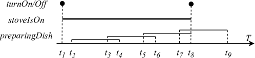
The starting point for many monitoring systems is Linear Temporal Logic (LTL) [25], where formulae are interpreted over single event sequences. This makes it difficult to incorporate concurrent activities such as, for instance, those carried out by a chef following some recipe to create a meal (see Figure 1). They may prepare multiples dishes of the same course in parallel, however the preparation of each dish happens on different overlapping intervals. This is difficult to formalise with logics that talk about single traces of events. Temporal logics that allow the representation of concurrent activities directly are those of Halpern and Shoham (HS) [17] and Allen’s Algebra [3]. Both logics are interpreted over sets of (possibly overlapping, discrete) time intervals, and model instantaneous events via point intervals ([t,t]).

Refer to caption
Figure 1: Example of instantaneous and durative temporal phenomena. ${\mathit{turnOn/Off}}$ is instantaneous and true when the stove is turned on/off, ${\mathit{stoveIsOn}}$ is durative and holds when the stove is on, and finally ${\mathit{preparingDish}}$ is also durative and holds when a dish is being prepared.

In previous work [23], we introduced a temporal logic similar to those of Halpern/Shoham and Allen, which is interpreted over separate (sets of) time intervals and instantaneous events, which was specifically designed for a maritime application domain. It allows to easily specify concurrent activities and related start and endpoints. Deliberately absent in our logics (and related prior ones) are explicit negations/complements of formulae that hold on overlapping intervals. We implemented an event processing system111https://manospits.github.io/Phenesthe/ and evaluated it on a real maritime monitoring scenario [24]—whereby maritime experts authored maritime phenomena of interest—proving that our system is capable of producing phenomena detections in real time.

In this work, we extend our language with two extra temporal modalities: minimal range ($\looparrowright$), and interval filtering ($\textsf{\small filter})$. The minimal range operator allows to capture durative temporal phenomena that start at the latest occurrence of a starting condition before the stopping condition, for example, the last working period of machine since someone operated it until it broke down. Filtering is very important for specifying the duration constraints of a temporal phenomenon, e.g., a steak is cooked rare if its on a hot pan for approximately 90 seconds on each side. Both examples are impossible to formalise in the original version of our temporal logic. It is evident that $\looparrowright$ has similar semantics to the ‘until’ operator of LTL. However, formulae that utilise ‘until’ are true on instants of time, while formulae that utilise ‘$\looparrowright$’ are true on intervals. While in terms of expressive power the two operators are similar, $\looparrowright$, in practice, allows efficient computations and more concise formulae. Similarly, in the case of filtering, writing an LTL formula for filtering periods based on some fixed threshold is possible, however the formula is not trivial and its length depends the threshold. Comparing LTL and our temporal logic, we show that the fragment of our original language that is comparable with LTL was at most as expressive as the pure past fragment of LTL, while the same fragment but with the addition of the ‘$\looparrowright$’ and ‘filter’ operators has equal expressive power to LTL. Concerning our full temporal logic, a comparison with LTL is impossible since the structures on which their respective semantics are based, are incomparable, however we show that our language is expressible in Dyadic First Order logic (DFO) and is strictly less expressive. As expected, including temporal modalities that involve the future requires additional steps for complex event processing. In order to guarantee that our extended implementation, Phenesthe+, is correct, inspired from runtime monitoring and verification [2, 6], we define criteria for proper stream processors of our language and discuss how Phenesthe+ conforms to them. Finally, we illustrate through experimental evaluation that the efficiency of Phenesthe+, is not significantly compromised. Therefore the contributions of this paper are:

  • We extend the expressiveness of our language for representing “look ahead happenings”,

  • We formally study the expressive power of the temporal logic introduced in [23] and its extension,

  • We define criteria for proper stream processors utilising our temporal logic,

  • We showcase that our stream processing engine is capable of performing real-time complex event processing by adopting a maritime surveillance use-case.

The paper is organised as follows. First in Section 2 we describe our temporal logic. Next, in Section 3 we illustrate through examples inspired by the maritime domain the usage of the new temporal modalities. In Section 4 we study the expressive power of our temporal logic. Then, in Section 5 we describe the requirements a stream processor should satisfy for processing formulae of our language, while in Section 6 we empirically evaluate Phenesthe+. Finally, in Section 7 we present work related to ours, summarise, and discuss further directions.

2 The Language of Phenesthe

The key components of our language are instantaneous events, durative disjoint states and durative, possibly non disjoint, dynamic temporal phenomena. In what follows, ‘temporal phenomena’ includes all of the three aforementioned categories.

Syntax. Formally, our Temporal Phenomena Definition Language (TPhL) is described by the triplet $\langle\mathcal{P}^{esd},L,\Phi\rangle$, where $\mathcal{P}^{esd}$ is a predicate set defined by the union of the event, state or dynamic temporal phenomenon predicates sets (in symbols $\mathcal{P}^{e/s/d}$ resp.); $L$ is a set defined by the union of the set of the logical connectives $\{\wedge,\vee,\neg,\in\}$, the set of temporal operators, $\{\rightarrowtail,\looparrowright,\sqcup,\sqcap,\setminus,\textsf{\small filter}_{\square}\}$ where the ‘$\square$’ symbol may be one of the following symbols ${\{<,\geq,=\}}$, the set of temporal relations $\{\textsf{\small before}$, meets, overlaps, finishes, starts, equals, $\textsf{\small contains}\}$ and finally the set of the $\{\textsf{\small start},\textsf{\small end}\}$ operators; $\Phi$ is the set of formulae defined by the union of the formulae sets $\Phi^{\mathchoice{\mathbin{\vbox{\hbox{\scalebox{0.5}{$\displaystyle\bullet$}}}}}{\mathbin{\vbox{\hbox{\scalebox{0.5}{$\textstyle\bullet$}}}}}{\mathbin{\vbox{\hbox{\scalebox{0.5}{$\scriptstyle\bullet$}}}}}{\mathbin{\vbox{\hbox{\scalebox{0.5}{$\scriptscriptstyle\bullet$}}}}}}$, $\Phi^{-}$ and $\Phi^{=}$. We assume that the set of predicate symbols includes those with atemporal and fixed semantics, such as arithmetic comparison operators etc., however for simplification reasons in what follows we omit their presentation. Formulae of $\Phi^{\mathchoice{\mathbin{\vbox{\hbox{\scalebox{0.5}{$\displaystyle\bullet$}}}}}{\mathbin{\vbox{\hbox{\scalebox{0.5}{$\textstyle\bullet$}}}}}{\mathbin{\vbox{\hbox{\scalebox{0.5}{$\scriptstyle\bullet$}}}}}{\mathbin{\vbox{\hbox{\scalebox{0.5}{$\scriptscriptstyle\bullet$}}}}}}$ describe instantaneous temporal phenomena, and formulae of $\Phi^{-}$ describe durative temporal phenomena that hold (are true) in disjoint maximal intervals, finally formulae of $\Phi^{=}$ describe durative temporal phenomena that may hold in non-disjoint intervals. Figure 1 shows an example of an event (${\mathit{turnOn/Off}}$), a state (${\mathit{stoveIsOn}}$) and a dynamic temporal phenomenon (${\mathit{preparingDish}}$).

Therefore given a set of event, state and dynamic phenomena predicates $\mathcal{P}^{esd}$ the formulae of TPhL are defined as follows:

$\displaystyle\phi$ $\displaystyle:=\phi^{\mathchoice{\mathbin{\vbox{\hbox{\scalebox{0.5}{$\displaystyle\bullet$}}}}}{\mathbin{\vbox{\hbox{\scalebox{0.5}{$\textstyle\bullet$}}}}}{\mathbin{\vbox{\hbox{\scalebox{0.5}{$\scriptstyle\bullet$}}}}}{\mathbin{\vbox{\hbox{\scalebox{0.5}{$\scriptscriptstyle\bullet$}}}}}}\ |\ \phi^{-}\ |\ \phi^{=}$
$\displaystyle\phi^{\mathchoice{\mathbin{\vbox{\hbox{\scalebox{0.5}{$\displaystyle\bullet$}}}}}{\mathbin{\vbox{\hbox{\scalebox{0.5}{$\textstyle\bullet$}}}}}{\mathbin{\vbox{\hbox{\scalebox{0.5}{$\scriptstyle\bullet$}}}}}{\mathbin{\vbox{\hbox{\scalebox{0.5}{$\scriptscriptstyle\bullet$}}}}}}$ $\displaystyle:=P^{e}(a_{1},...,a_{k})\ |\ \neg\phi^{\mathchoice{\mathbin{\vbox{\hbox{\scalebox{0.5}{$\displaystyle\bullet$}}}}}{\mathbin{\vbox{\hbox{\scalebox{0.5}{$\textstyle\bullet$}}}}}{\mathbin{\vbox{\hbox{\scalebox{0.5}{$\scriptstyle\bullet$}}}}}{\mathbin{\vbox{\hbox{\scalebox{0.5}{$\scriptscriptstyle\bullet$}}}}}}\ |\ \phi^{\mathchoice{\mathbin{\vbox{\hbox{\scalebox{0.5}{$\displaystyle\bullet$}}}}}{\mathbin{\vbox{\hbox{\scalebox{0.5}{$\textstyle\bullet$}}}}}{\mathbin{\vbox{\hbox{\scalebox{0.5}{$\scriptstyle\bullet$}}}}}{\mathbin{\vbox{\hbox{\scalebox{0.5}{$\scriptscriptstyle\bullet$}}}}}}\ [\wedge,\vee]\ \phi^{\mathchoice{\mathbin{\vbox{\hbox{\scalebox{0.5}{$\displaystyle\bullet$}}}}}{\mathbin{\vbox{\hbox{\scalebox{0.5}{$\textstyle\bullet$}}}}}{\mathbin{\vbox{\hbox{\scalebox{0.5}{$\scriptstyle\bullet$}}}}}{\mathbin{\vbox{\hbox{\scalebox{0.5}{$\scriptscriptstyle\bullet$}}}}}}\ |\ \textsf{\small start}(\phi^{-})\ |\ \textsf{\small end}(\phi^{-})\ |\ \phi^{\mathchoice{\mathbin{\vbox{\hbox{\scalebox{0.5}{$\displaystyle\bullet$}}}}}{\mathbin{\vbox{\hbox{\scalebox{0.5}{$\textstyle\bullet$}}}}}{\mathbin{\vbox{\hbox{\scalebox{0.5}{$\scriptstyle\bullet$}}}}}{\mathbin{\vbox{\hbox{\scalebox{0.5}{$\scriptscriptstyle\bullet$}}}}}}\in\phi^{-}$
$\displaystyle\phi^{-}$ $\displaystyle:=P^{s}(a_{1},...,a_{k})\ |\phi^{\mathchoice{\mathbin{\vbox{\hbox{\scalebox{0.5}{$\displaystyle\bullet$}}}}}{\mathbin{\vbox{\hbox{\scalebox{0.5}{$\textstyle\bullet$}}}}}{\mathbin{\vbox{\hbox{\scalebox{0.5}{$\scriptstyle\bullet$}}}}}{\mathbin{\vbox{\hbox{\scalebox{0.5}{$\scriptscriptstyle\bullet$}}}}}}\ [\rightarrowtail,\looparrowright]\ \phi^{\mathchoice{\mathbin{\vbox{\hbox{\scalebox{0.5}{$\displaystyle\bullet$}}}}}{\mathbin{\vbox{\hbox{\scalebox{0.5}{$\textstyle\bullet$}}}}}{\mathbin{\vbox{\hbox{\scalebox{0.5}{$\scriptstyle\bullet$}}}}}{\mathbin{\vbox{\hbox{\scalebox{0.5}{$\scriptscriptstyle\bullet$}}}}}}\ |\ \phi^{-}\ [\sqcup,\sqcap,\setminus]\ \phi^{-}|\phi^{-}\textsf{\small filter}\ n\ (\text{where}\ n\in\mathbb{N}\cup\{\infty\})$
$\displaystyle\phi^{=}$ $\displaystyle:=P^{d}(a_{1},...,a_{k})\ |\ [\phi^{-},\phi^{=}]\ [\textsf{\small meets},\textsf{\small overlaps},\textsf{\small equals}]\ [\phi^{-},\phi^{=}]$
$\displaystyle\quad\qquad|\ [\phi^{\mathchoice{\mathbin{\vbox{\hbox{\scalebox{0.5}{$\displaystyle\bullet$}}}}}{\mathbin{\vbox{\hbox{\scalebox{0.5}{$\textstyle\bullet$}}}}}{\mathbin{\vbox{\hbox{\scalebox{0.5}{$\scriptstyle\bullet$}}}}}{\mathbin{\vbox{\hbox{\scalebox{0.5}{$\scriptscriptstyle\bullet$}}}}}},\phi^{-},\phi^{=}]\ [\textsf{\small starts},\textsf{\small finishes}]\ [\phi^{-},\phi^{=}]$
$\displaystyle\quad\qquad|\ [\phi^{-},\phi^{=}]\ \textsf{\small contains}\ [\phi^{\mathchoice{\mathbin{\vbox{\hbox{\scalebox{0.5}{$\displaystyle\bullet$}}}}}{\mathbin{\vbox{\hbox{\scalebox{0.5}{$\textstyle\bullet$}}}}}{\mathbin{\vbox{\hbox{\scalebox{0.5}{$\scriptstyle\bullet$}}}}}{\mathbin{\vbox{\hbox{\scalebox{0.5}{$\scriptscriptstyle\bullet$}}}}}},\phi^{-},\phi^{=}]$
$\displaystyle\quad\qquad|\ [\phi^{\mathchoice{\mathbin{\vbox{\hbox{\scalebox{0.5}{$\displaystyle\bullet$}}}}}{\mathbin{\vbox{\hbox{\scalebox{0.5}{$\textstyle\bullet$}}}}}{\mathbin{\vbox{\hbox{\scalebox{0.5}{$\scriptstyle\bullet$}}}}}{\mathbin{\vbox{\hbox{\scalebox{0.5}{$\scriptscriptstyle\bullet$}}}}}},\phi^{-},\phi^{=}]\ \textsf{\small before}\ [\phi^{\mathchoice{\mathbin{\vbox{\hbox{\scalebox{0.5}{$\displaystyle\bullet$}}}}}{\mathbin{\vbox{\hbox{\scalebox{0.5}{$\textstyle\bullet$}}}}}{\mathbin{\vbox{\hbox{\scalebox{0.5}{$\scriptstyle\bullet$}}}}}{\mathbin{\vbox{\hbox{\scalebox{0.5}{$\scriptscriptstyle\bullet$}}}}}},\phi^{-},\phi^{=}]$

where $a_{1},...,a_{k}$ correspond to terms denoting atemporal properties.

Semantics. We assume time is discrete and represented by the natural numbers $T=\mathbb{N}$ ordered via the ‘$<$’ relation. In what follows we assume that for all models discussed in this paper time is represented by $\mathbb{N}$. For the formulae sets $\Phi^{\mathchoice{\mathbin{\vbox{\hbox{\scalebox{0.5}{$\displaystyle\bullet$}}}}}{\mathbin{\vbox{\hbox{\scalebox{0.5}{$\textstyle\bullet$}}}}}{\mathbin{\vbox{\hbox{\scalebox{0.5}{$\scriptstyle\bullet$}}}}}{\mathbin{\vbox{\hbox{\scalebox{0.5}{$\scriptscriptstyle\bullet$}}}}}},\Phi^{-}$ and $\Phi^{=}$ we define the model $\mathcal{M}=\langle T,I,<,V^{\mathchoice{\mathbin{\vbox{\hbox{\scalebox{0.5}{$\displaystyle\bullet$}}}}}{\mathbin{\vbox{\hbox{\scalebox{0.5}{$\textstyle\bullet$}}}}}{\mathbin{\vbox{\hbox{\scalebox{0.5}{$\scriptstyle\bullet$}}}}}{\mathbin{\vbox{\hbox{\scalebox{0.5}{$\scriptscriptstyle\bullet$}}}}}},V^{-},V^{=}\rangle$ where $V^{\mathchoice{\mathbin{\vbox{\hbox{\scalebox{0.5}{$\displaystyle\bullet$}}}}}{\mathbin{\vbox{\hbox{\scalebox{0.5}{$\textstyle\bullet$}}}}}{\mathbin{\vbox{\hbox{\scalebox{0.5}{$\scriptstyle\bullet$}}}}}{\mathbin{\vbox{\hbox{\scalebox{0.5}{$\scriptscriptstyle\bullet$}}}}}}:\mathcal{P}^{e}\rightarrow 2^{T}$, $V^{-}:\mathcal{P}^{s}\rightarrow 2^{I}$, $V^{=}:\mathcal{P}^{d}\rightarrow 2^{I}$ are valuations, and $I=\{[ts,te]:ts<te\ \text{and}\ ts,te\in T\}\cup\{[ts,\infty):ts\in T\}$ is the set of time intervals of $T$. Intervals of the form $[ts,\infty)$ denote that a phenomenon started being true at $ts$, and continues being true forever. Intervals of the form $[ts,te]$ denote that a phenomenon started being true at $ts$ and stopped being true at $te$. In what follows, we will use the abbreviated version for bounded quantifiers, i.e., $\forall_{>z_{1}}^{<z_{2}}x(...)$ denotes $\forall x\ (x>z_{1}\wedge x<z_{2})\rightarrow(...)$, and $\exists_{>z_{1}}^{<z_{2}}x(...)$ denotes $\exists x\ (x>z_{1}\wedge x<z_{2})\wedge(...)$.

Given a model $\mathcal{M}$, the validity of a formula $\phi\in\Phi^{\mathchoice{\mathbin{\vbox{\hbox{\scalebox{0.5}{$\displaystyle\bullet$}}}}}{\mathbin{\vbox{\hbox{\scalebox{0.5}{$\textstyle\bullet$}}}}}{\mathbin{\vbox{\hbox{\scalebox{0.5}{$\scriptstyle\bullet$}}}}}{\mathbin{\vbox{\hbox{\scalebox{0.5}{$\scriptscriptstyle\bullet$}}}}}}$ at a timepoint $t\in T$ (in symbols $\mathcal{M},t\models\phi$) is determined by the rules below, starting with the boolean connectives.

  • $\mathcal{M},t\models P^{e}(a_{1},...,a_{n})$ iff $t\in$ $V^{\mathchoice{\mathbin{\vbox{\hbox{\scalebox{0.5}{$\displaystyle\bullet$}}}}}{\mathbin{\vbox{\hbox{\scalebox{0.5}{$\textstyle\bullet$}}}}}{\mathbin{\vbox{\hbox{\scalebox{0.5}{$\scriptstyle\bullet$}}}}}{\mathbin{\vbox{\hbox{\scalebox{0.5}{$\scriptscriptstyle\bullet$}}}}}}(P^{e}(a_{1},...,a_{n}))$.

  • $\mathcal{M},t\models\neg\phi$ iff $\mathcal{M},t\not\models\phi$.

  • $\mathcal{M},t\models\phi[\wedge,\vee]\psi$ iff $\mathcal{M},t\models\phi$ [and, or]$\ \mathcal{M},t\models\psi$.

Next we define the semantics for $\textsf{\small start},\textsf{\small end}$ and $\in$ which allow interaction between formulae of $\Phi^{\mathchoice{\mathbin{\vbox{\hbox{\scalebox{0.5}{$\displaystyle\bullet$}}}}}{\mathbin{\vbox{\hbox{\scalebox{0.5}{$\textstyle\bullet$}}}}}{\mathbin{\vbox{\hbox{\scalebox{0.5}{$\scriptstyle\bullet$}}}}}{\mathbin{\vbox{\hbox{\scalebox{0.5}{$\scriptscriptstyle\bullet$}}}}}}$ and $\Phi^{-}$ via the starting, ending, and intermediate points of intervals at which $\Phi^{-}$ formulae hold.

  • $\mathcal{M},t\models\textsf{\small start}(\phi)$ iff $\exists te.\ \mathcal{M},[t,te]\models\phi$ or $\mathcal{M},[t,\infty)\models\phi$, where $\mathcal{M},[t,te]\models\phi$ denotes the validity of a formula $\phi\in\Phi^{-}$ at an interval $[t,te]$ as defined below.

  • $\mathcal{M},t\models\textsf{\small end}(\phi)$ iff $\exists ts.\ \mathcal{M},[ts,t]\models\phi$.

  • $\mathcal{M},t\models\phi\in\psi$ iff $\mathcal{M},t\models\phi$ and $\exists^{\leq t}ts.\exists_{\geq t}te.\ \mathcal{M},[ts,te]\models\psi$.

Given a model $\mathcal{M}$, the validity of a formula $\phi\in\Phi^{-}$ at a time interval $i=[ts,te]\in I$ (in symbols $\mathcal{M},[ts,te]\models\phi$) is defined as follows. We start with the $\looparrowright$ and $\rightarrowtail$ operators which allow specifying minimal or maximal intervals between instants where formulae of $\Phi^{\mathchoice{\mathbin{\vbox{\hbox{\scalebox{0.5}{$\displaystyle\bullet$}}}}}{\mathbin{\vbox{\hbox{\scalebox{0.5}{$\textstyle\bullet$}}}}}{\mathbin{\vbox{\hbox{\scalebox{0.5}{$\scriptstyle\bullet$}}}}}{\mathbin{\vbox{\hbox{\scalebox{0.5}{$\scriptscriptstyle\bullet$}}}}}}$ are true.

  • $\mathcal{M},i\models P^{s}(a_{1},...,a_{n})$ iff $i\in$ $V^{-}(P^{s}(a_{1},...,a_{n}))$.

  • $\mathcal{M},[ts,te]\models\phi\looparrowright\psi$ iff $\mathcal{M},ts\models\phi$ and $\mathcal{M},te\models\psi\wedge\neg\phi$ and $\forall_{>ts}^{<te}t.\bigl{[}\mathcal{M},t\not\models\phi$ and $\mathcal{M},t\not\models\psi\wedge\neg\phi\bigr{]}$. Therefore, $\phi\looparrowright\psi$ holds for the intervals that start at the latest instant $ts$ at which $\phi$ is true and end at first instant $te$ after $ts$ where $\psi\wedge\neg\phi$ is true.

  • $\mathcal{M},[ts,te]\models\phi\rightarrowtail\psi$ iff $\mathcal{M},ts\models\phi$ and $\mathcal{M},te\models\psi\wedge\neg\phi$ and $\forall_{>ts}^{<te}t.\ \mathcal{M},t\not\models\psi\wedge\neg\phi$ and $\forall^{<ts}ts^{\prime}.$ $\mathcal{M},ts^{\prime}\models\phi\rightarrow\exists^{<ts}_{>ts^{\prime}}te^{\prime}.\ \mathcal{M},te^{\prime}\models\psi\wedge\neg\phi$.

    Essentially, $\phi\rightarrowtail\psi$ holds for the disjoint maximal intervals that start at the earliest instant $ts$ where $\phi$ is true and end at the earliest instant $te$ where $\psi$ is true and $\phi$ is false.

  • $\mathcal{M},[ts,\infty)\models\phi\rightarrowtail\psi$ iff $\mathcal{M},ts\models\phi$ and $\forall_{>ts}t.\ \mathcal{M},t\not\models\psi\wedge\neg\phi$ and $\forall^{<ts}ts^{\prime}.\ \mathcal{M},ts^{\prime}\models\phi\rightarrow\exists^{<ts}_{>ts^{\prime}}te^{\prime}.$ $\mathcal{M},te\models\psi\wedge\neg\phi$.

    Therefore a formula $\phi\rightarrowtail\psi$ may hold indefinitely if there does not exist an instant after $ts$ at which $\psi\wedge\neg\phi$ is satisfied. For simplification reasons in the semantics below we omit intervals open at the right to infinity since they can be treated in a similar manner.

We continue with the definition of semantics for $\sqcup,\sqcap$ and $\setminus$ which correspond to the usual set operations but for time intervals.

  • $\mathcal{M},[ts,te]\models\phi\ \sqcup\ \psi$ iff222A first order definition of the semantics of $\sqcup$ is possible but more lengthy.

    • exists a sequence of length $k>1$ of intervals $i_{1},...,i_{k}\in I$ where $i_{k}=[ts_{k},te_{k}]$, $ts=ts_{1}$ and $te=te_{k}$ such that:

      1. 1.

        $\forall\alpha\in[1,k-1]$: $te_{\alpha}\in i_{\alpha+1}$, $ts_{\alpha}<ts_{\alpha+1}$ and $te_{\alpha}<te_{\alpha+1}$ ,

      2. 2.

        $\forall\beta\in[1,k]$: $\mathcal{M},[ts_{\beta},te_{\beta}]\models\phi$ or $\mathcal{M},[ts_{\beta},te_{\beta}]\models\psi$, and

      3. 3.

        $\nexists i_{\gamma}=[ts_{\gamma},te_{\gamma}]\in I-\{i_{1},...,i_{k}\}$ where $\mathcal{M},[ts_{\gamma},te_{\gamma}]\models\phi$ or $\mathcal{M},[ts_{\gamma},te_{\gamma}]\models\psi$ and $ts_{1}\in i_{\gamma}$ or $te_{k}\in i_{\gamma}$

    • or, $\mathcal{M},[ts,te]\models\phi$ or $\mathcal{M},[ts,te]\models\psi$ and $\nexists i_{\gamma}=[ts_{\gamma},te_{\gamma}]\in I-\{[ts,te]\}$ where $\mathcal{M},[ts_{\gamma},te_{\gamma}]\models\phi$ or $\mathcal{M},[ts_{\gamma},te_{\gamma}]\models\psi$ and $ts\in i_{\gamma}$ or $te\in i_{\gamma}$.

    For a sequence of intervals, conditions (1-2) ensure that intervals, at which $\phi$ or $\psi$ are valid, overlap or touch will coalesce, while condition (3) ensures that the resulting interval is maximal. In the case of a single interval, the conditions ensure that at the interval $[ts,te]$ $\phi$ or $\psi$ is valid, and that $[ts,te]$ is maximal. In simple terms, the temporal union $\phi\ \sqcup\ \psi$ holds for the intervals where at least one of $\phi$ or $\psi$ hold. The above definition of temporal union follows the definitions of temporal coalescing presented in [9, 15].

  • $\mathcal{M},[ts,te]\models\phi\ \setminus\ \psi$ iff $\exists[ts^{\prime},te^{\prime}]\in I$ where $\mathcal{M},[ts^{\prime},te^{\prime}]\models\phi$, $[ts,te]\subseteq[ts^{\prime},te^{\prime}]$ (i.e., $[ts,te]$ subinterval of $[ts^{\prime},te^{\prime}]$), $\forall[ts_{\psi},te_{\psi}]\in I$ where $\mathcal{M},[ts_{\psi},te_{\psi}]\models\psi$, $[ts,te]\cap[ts_{\psi},te_{\psi}]=\varnothing$ and finally $[ts,te]$ is maximal. In plain language, the temporal difference of formulae $\phi,\psi$ holds for the maximal subintervals of the intervals at which $\phi$ holds but $\psi$ doesn’t hold.

  • $\mathcal{M},[ts,te]\models\phi\ \sqcap\ \psi$ iff $\exists[ts_{\phi},te_{\phi}],[ts_{\psi},te_{\psi}]\in I$ where $\mathcal{M},[ts_{\phi},te_{\phi}]\models\phi$, $\mathcal{M},[ts_{\psi},te_{\psi}]\models\psi$ and $\exists[ts,te]\in I$ where $[ts,te]\subseteq[ts_{\phi},te_{\phi}]$, $[ts,te]\subseteq[ts_{\psi},te_{\psi}]$ and $[ts,te]$ is maximal. In other words, the temporal intersection of two formulae of $\Phi^{-}$ holds for the intervals at which both formulae hold.

We finish the semantics for formulae of $\Phi^{-}$, with the semantics of the filter operator, which allows specifying constraints on the length of intervals at which formulae of $\Phi^{-}$ hold.

  • $\mathcal{M},[ts,te]\models\phi\ \textsf{\small filter}_{\{<,\geq,=\}}\ n$ iff $\mathcal{M},[ts,te]\models\phi$ and $te-ts\ {\{<,\geq,=\}}\ n$.

Due to space limitations and for this part only we will adopt point intervals to refer to instants. This will allow us to define the semantics for formulae of $\Phi^{=}$ without specifying different rules for involved sub-formulae of $\Phi^{\mathchoice{\mathbin{\vbox{\hbox{\scalebox{0.5}{$\displaystyle\bullet$}}}}}{\mathbin{\vbox{\hbox{\scalebox{0.5}{$\textstyle\bullet$}}}}}{\mathbin{\vbox{\hbox{\scalebox{0.5}{$\scriptstyle\bullet$}}}}}{\mathbin{\vbox{\hbox{\scalebox{0.5}{$\scriptscriptstyle\bullet$}}}}}}$. In other words given a $\phi\in\Phi^{\mathchoice{\mathbin{\vbox{\hbox{\scalebox{0.5}{$\displaystyle\bullet$}}}}}{\mathbin{\vbox{\hbox{\scalebox{0.5}{$\textstyle\bullet$}}}}}{\mathbin{\vbox{\hbox{\scalebox{0.5}{$\scriptstyle\bullet$}}}}}{\mathbin{\vbox{\hbox{\scalebox{0.5}{$\scriptscriptstyle\bullet$}}}}}}$ we will denote the satisfaction relation $\mathcal{M},t\models\phi$ as $\mathcal{M},[t,t]\models\phi$. Given a model $\mathcal{M}$, the validity of a formula $\phi\in\Phi^{=}$ at a time interval $[ts,te]\in I$ (in symbols $\mathcal{M},[ts,te]\models\phi$) is defined as follows:

  • $\mathcal{M},[ts,te]\models P^{d}(a_{1},...,a_{n})$ iff $[ts,te]\in V^{=}(P^{d}(a_{1},...,a_{n}))$.

  • $\mathcal{M},[ts,te]\models\phi\ \textsf{\small before}\ \psi$ iff $\exists te^{\prime}.\exists_{>te^{\prime}}ts^{\prime}.\bigl{[}\mathcal{M},[ts,te^{\prime}]\models\phi$ and $\mathcal{M},[ts^{\prime},te]\models\psi$ and $\forall ts^{\prime\prime}.\forall_{>te^{\prime}}^{<ts^{\prime}}te^{\prime\prime}.$ $\mathcal{M},[ts^{\prime\prime},te^{\prime\prime}]\not\models\phi$ and $\forall_{>te^{\prime}}^{<ts^{\prime}}ts^{\prime\prime}.\forall te^{\prime\prime}.\mathcal{M},[ts^{\prime\prime},te^{\prime\prime}]\not\models\psi\bigr{]}$. In our approach the ‘before’ relation holds only for intervals where the pair of instants or intervals at which the participating formulae are true or hold, are contiguous. For example, for the intervals $[1,2]$, $[1,3]$ and $[5,6]$ only $[1,3]$ is before $[5,6]$. We chose to limit the intervals satisfying the before relation, as in practice it is usually the case that the interval directly before another one is required for specifying a dynamic phenomenon.

  • $\mathcal{M},[ts,te]\models\phi\ \textsf{\small meets}\ \psi$ iff $\exists t.\mathcal{M},[ts,t]\models\phi$ and $\mathcal{M},[t,te]\models\psi$.

  • $\mathcal{M},[ts,te]\models\phi\ \textsf{\small overlaps}\ \psi$ iff $\exists_{>ts}^{<te}ts^{\prime}.\exists_{>ts^{\prime}}^{<te}te^{\prime}.\bigl{[}\mathcal{M},[ts,te^{\prime}]\models\phi$ and $\mathcal{M},[ts^{\prime},te]\models\psi\bigr{]}$.

  • $\mathcal{M},[ts,te]\models\phi\ \textsf{\small finishes}\ \psi$ iff $\exists_{>ts}^{\leq te}ts^{\prime}.\bigl{[}\mathcal{M},[ts^{\prime},te]\models\phi$ and $\mathcal{M},[ts,te]\models\psi\bigr{]}$.

  • $\mathcal{M},[ts,te]\models\phi\ \textsf{\small starts}\ \psi$ iff $\exists^{<te}_{\geq ts}te^{\prime}.\bigl{[}\mathcal{M},[ts,te^{\prime}]\models\phi$ and $\mathcal{M},[ts,te]\models\psi\bigr{]}$.

  • $\mathcal{M},[ts,te]\models\phi\ \textsf{\small equals}\ \psi$ iff $\mathcal{M},[ts,te]\models\phi$ and $\mathcal{M},[ts,te]\models\psi$.

  • $\mathcal{M},[ts,te]\models\phi\ \textsf{\small contains}\ \psi$ iff $\mathcal{M},[ts,te]\models\phi$ and $\exists_{>ts}ts^{\prime}.\exists^{<te}te^{\prime}.$ $\mathcal{M},[ts^{\prime},te^{\prime}]\models\psi$.

3 Examples of maritime properties expressed in TPhL

We demonstrate the usability of TPhL and the new temporal modalities by adopting a maritime monitoring scenario. When it comes to maritime surveillance there are several resources available; for example the Automatic Identification System (AIS) allows the transmission of timestamped positional and ancillary data from vessels, maritime areas in the form of polygons can be used for producing vessel-area relations and so on. Similar to [23], we assume the input consists of AIS messages along with spatial events relating vessels to areas of interest e.g., port areas, fishing areas and so on. Therefore our task here involves detecting maritime phenomena of interest i.e., the instants, time periods at which they are true over a maritime input stream. Below we formalise some maritime temporal phenomena333The complete set of definitions is available in our online repository https://github.com/manospits/Phenesthe/tree/future. that utilise the new temporal modalities ($\looparrowright$ and filter).

Fishing warning. Illegal fishing is a very important issue. Vessels engaged in illegal fishing typically declare fake ship-types. Consider the formalisation below for detecting suspicious stops in fishing areas.

$\displaystyle\textsf{\small state\_phenomenon}\ {\mathit{fishing\_warning(V,F)}}:$
$\displaystyle\quad(({\mathit{in\_fishing\_area}}(V,F)\wedge\neg{\mathit{vessel\_type(V,fishing)}})\ \sqcap\ stopped(V))\ \textsf{\small filter}_{\geq}600.$

state_phenomenon is a keyword for declaring the phenomenon type, ${\mathit{in\_fishing\_area}}$ is a user defined state that holds for the time periods a vessel $V$ is within a fishing area $F$, while ${\mathit{stopped}}$ is a state that holds for the time periods a vessel is stopped. Finally, ${\mathit{vessel\_type}}(V,T)$ is an atemporal predicate that is true when vessel $V$ has type $T$. Therefore, a vessel performs a ${\mathit{fishing\_warning}}$, if it is not a fishing vessel, and it is stopped within a fishing area for a period longer that 10 min (600 sec). Here, filtering is used for minimising false detections occurring from AIS errors (e.g., zero speed) or normal activities.

Port waiting time. Monitoring the waiting time of vessels since they entered a port and until they get moored is highly useful for various operational and logistical reasons (e.g., efficient planning of resources). However, some vessels may enter and leave a port without mooring—due to weather conditions for example. We formalise port waiting time below.

$\displaystyle\textsf{\small state\_phenomenon}\ {\mathit{waiting\_time}}(V,P):$
$\displaystyle\quad\textsf{\small start}({\mathit{in\_port}}(V,P))\looparrowright\textsf{\small start}({\mathit{moored}}(V,P)).$

${\mathit{in\_port}}$ is a state that holds when a vessel is in a port, while ${\mathit{moored}}$ is a state that holds when a vessel is moored at a port. Note that the left and right arguments of $\looparrowright$ are formulae of $\Phi^{\mathchoice{\mathbin{\vbox{\hbox{\scalebox{0.5}{$\displaystyle\bullet$}}}}}{\mathbin{\vbox{\hbox{\scalebox{0.5}{$\textstyle\bullet$}}}}}{\mathbin{\vbox{\hbox{\scalebox{0.5}{$\scriptstyle\bullet$}}}}}{\mathbin{\vbox{\hbox{\scalebox{0.5}{$\scriptscriptstyle\bullet$}}}}}}$, therefore if these formulae were used in other definitions we could have defined corresponding events. Consequently, the ${\mathit{waiting\_time}}$ state holds for the minimal periods between the time a vessel enters a port and the time the vessel starts being moored. Here we are interested in the minimal period, as we want to detect only the cases where a vessel entered a port and got moored.

4 Expressiveness

In this section we study the expressive power of our language. We consider three syntactic fragments of TPhL. The first one, denoted as TPhL${}_{o}^{-}$, corresponds to the original version of the language (w/o $\looparrowright,\textsf{\small filter}$) and excluding formulae of $\Phi^{=}$ (recall that $\Phi^{=}$ formulae hold on possibly non-disjoint intervals). The second is TPhL-, which is the same as TPhL${}_{o}^{-}$ but includes $\looparrowright$ and filter, while the third, TPhL  corresponds to the complete language. Figure 2 (left) illustrates the syntactic relation between TPhL, TPhL- and TPhL${}^{-}_{o}$. In more detail, we will show that TPhL${}_{o}^{-}$ is equally expressive as pure past LTL, TPhL- has equal expressive power to LTL, and finally TPhL is strictly less expressive than DFO. The relations in terms of expressive power between the different language fragments are illustrated in Figure 2 (right).

4.1 Preliminaries

Before we continue with our analysis, as a reminder we present the syntax of LTL with past, and First Order Monadic Logic of Order (FOMLO).

Refer to caption
TPhL-TPhL${}_{o}^{-}$DFOTPhLLTL$[\texttt{Y}\texttt{S}]$LTL$[\texttt{X}\texttt{U},\texttt{Y}\texttt{S}]$
Figure 2: Syntactic relation between the fragments of TPhL (left). Expressive relations between different fragments of TPhL, LTL and DFO (right). A fragment $A$ is strictly more expressive from a fragment $B$ if they are connected via $A\rightarrow B$. Double lined edges denote equal expressive power.

LTL. The formulae of LTL$[\texttt{X}\texttt{U},\texttt{Y}\texttt{S}]$, given a set of propositions $\mathcal{P}$ are defined as follows:

$\displaystyle\phi::=\ \perp\ |\ p\ |\ \neg\phi_{1}\ |\ \phi_{1}\wedge\phi_{2}\ |\ \texttt{X}\phi_{1}\ |\ \phi_{1}\ \texttt{U}\ \phi_{2}\ |\ \texttt{Y}\phi_{1}\ |\ \phi_{1}\ \texttt{S}\ \phi_{2};$

where X, and U stand for the next and until modalities, while Y, and S stand for previous and since. The formulae of LTL$[\texttt{X}\texttt{U},\texttt{Y}\texttt{S}]$ are interpreted over a discrete, linear model of time, formally represented as $\mathcal{M}_{TL}=\langle T,<,V^{TL}\rangle$, where $T$ is equal to $\mathbb{N}$, $<$ is the linear order and $V^{TL}:\mathcal{P}\rightarrow 2^{T}$ is the interpretation function, mapping each proposition to a set of time instants. The satisfaction relation, i.e., that a formula $\phi$ is true at $t$, is defined as $\mathcal{M}_{TL},t\models\phi$. The semantics of LTL are defined as usual; more specifically in what follows we assume the reflexive444As we work with discrete linear orders, this choice makes no difference. semantics of S and U. We denote the pure past fragment of LTL i.e., LTL without X and U as LTL[YS].

FOMLO. Given a countable set of variables ${x,y,z,...}$, the formulae of FOMLO over a set of unary predicate symbols $\Sigma$ are defined a follows:

$\displaystyle\mathit{atomic}::=x<y\ |\ x=y\ |\ P(x)\ (\text{where}\ P\in\Sigma)$
$\displaystyle\phi::=\mathit{atomic}\ |\ \neg\phi_{1}\ |\ \phi_{1}\vee\phi_{2}\ |\ \phi_{1}\wedge\phi_{2}\ |\ \exists x.\ \phi_{1}\ |\ \forall x.\ \phi_{1}$

We interpret FOMLO formulae over structures of the form $\mathcal{M}_{FO}\langle T,<,V^{FO}\rangle$, where $T$ is equal to $\mathbb{N}$, ‘$<$’ is the linear order while $V^{FO}:\Sigma\rightarrow 2^{T}$ is the interpretation of $\Sigma$. $\mathcal{M}_{FO},t_{1},t_{2},\cdots,t_{n}\models\phi(x_{1},x_{2},\cdots,x_{n})$ denotes the satisfaction of a formula $\phi$ with free variables $x_{1},x_{2},\cdots,x_{n}$ when they are interpreted as elements $t_{i}$ of $\mathcal{M}_{FO}$. The semantics of the formulae are defined as usual (see for example [26]). We also define the FOMLO- fragment of FOMLO. Syntactically a formula with one free variable $\phi(x)$, is a formula of the fragment if any bounded variable in the negated normal form of $\phi(x)$ is bounded to be $\leq x$. Semantically, this means that for all models a formula $\phi(x)$ of FOMLO- satisfies:

$\displaystyle\begin{array}[]{l}\forall t\ \mathcal{M}_{FO},t\ \models\phi(x)\leftrightarrow\mathcal{M}_{FO}[0,t],t\models\phi(x)\end{array}$ (2)

where ${M}_{FO}[0,t]$ is a finite model starting from 00 and ending up to position $t$ inclusive. Intuitively, formulae of FOMLO- can talk only about the past and the present. In what follows, given a set of propositions $\mathcal{P}=\{p_{1},...,p_{k}\}$ and a set of predicate symbols $\Sigma=\{p_{1}(x),...,p_{k}(x)\}$ a FOMLO model $\mathcal{M}_{FO}$ is faithful to $\mathcal{M}_{TL}$ iff $\forall_{\geq 1}^{\leq k}i.V^{FO}(p_{i}(x))=V^{TL}(p_{i})$.

DFO. Finally, on our expressiveness analysis we will also consider DFO, which in contrast to FOMLO, uses dyadic predicate symbols e.g., $p(x,y)$.

4.2 TPhL${}_{o}^{-}$ and Pure Past LTL

In this section we will show that TPhL${}_{o}^{-}$ is expressively equal to the pure past fragment of LTL, i.e., LTL$[\texttt{Y}\texttt{S}]$. The TPhL${}_{o}^{-}$ fragment is described by the triplet $\langle\mathcal{P}^{es},L^{-}_{o},\Phi\rangle$, where $\mathcal{P}^{es}$ is a set defined by the union of event and state predicate sets ($\mathcal{P}^{e/s}$); $L^{-}_{o}$ is a set defined by the union of the set of the logical connectives $\{\wedge,\vee,\neg,\in\}$ and the set of temporal operators $\{\rightarrowtail,\sqcup,\sqcap,\setminus\}$. Formulae TPhL${}_{o}^{-}$ are evaluated over $\mathcal{M}^{-}=\langle T,I,<,V^{\mathchoice{\mathbin{\vbox{\hbox{\scalebox{0.5}{$\displaystyle\bullet$}}}}}{\mathbin{\vbox{\hbox{\scalebox{0.5}{$\textstyle\bullet$}}}}}{\mathbin{\vbox{\hbox{\scalebox{0.5}{$\scriptstyle\bullet$}}}}}{\mathbin{\vbox{\hbox{\scalebox{0.5}{$\scriptscriptstyle\bullet$}}}}}},V^{-}\rangle$ models which are defined in a similar manner to the models presented in Section 2.

Given a finite set of event propositions555In what follows, for simplicity, we will refer to atomic predicates of TPhL as propositions. $\mathcal{P}^{e}=\{e_{1},...,e_{k}\}$, and a finite set of state propositions $\mathcal{P}^{s}=\{s_{1},...,s_{k}\}$ we say the FOMLO- model $M_{FO}=\langle T,<,V^{FO}\rangle$ is faithful to the model $\mathcal{M}^{-}=\langle T,I,<,V^{\mathchoice{\mathbin{\vbox{\hbox{\scalebox{0.5}{$\displaystyle\bullet$}}}}}{\mathbin{\vbox{\hbox{\scalebox{0.5}{$\textstyle\bullet$}}}}}{\mathbin{\vbox{\hbox{\scalebox{0.5}{$\scriptstyle\bullet$}}}}}{\mathbin{\vbox{\hbox{\scalebox{0.5}{$\scriptscriptstyle\bullet$}}}}}},V^{-}\rangle$ of TPhL${}_{o}^{-}$ if it has the following properties:

  • for any proposition $e$ in $\mathcal{P}^{e}$, $V^{\mathchoice{\mathbin{\vbox{\hbox{\scalebox{0.5}{$\displaystyle\bullet$}}}}}{\mathbin{\vbox{\hbox{\scalebox{0.5}{$\textstyle\bullet$}}}}}{\mathbin{\vbox{\hbox{\scalebox{0.5}{$\scriptstyle\bullet$}}}}}{\mathbin{\vbox{\hbox{\scalebox{0.5}{$\scriptscriptstyle\bullet$}}}}}}(e)=V^{FO}(e_{t})$, and

  • for any proposition $s$ in $\mathcal{P}^{s}$, $V^{-}(s)=\rho(V^{FO}(s_{+}),V^{FO}(s_{\in}),V^{FO}(s_{-}))$

where $e_{t}$ corresponds to the monadic predicate $e_{t}(x)$ and the triplet ($s_{+},s_{\in},s_{-}$) corresponds to the monadic predicates $s_{+}(x)$, $s_{\in}(x)$, $s_{+}(x)$ which are true on instants corresponding to the start, intermediate, and end of an interval respectively at which $s$ is true. $\rho:2^{T}\times 2^{T}\times 2^{T}\rightarrow 2^{I}$ is a partial mapping from three set of points to a set of intervals of $I$. Given three sets $S,B$ and $E$, corresponding to starting, intermediate and ending points resp., $\rho$ is defined as follows:

$\displaystyle\rho(S,B,E)=\ \begin{aligned} &\bigl{\{}[ts,te]:ts<te\wedge ts\in S\wedge te\in E\wedge\forall_{>ts}^{<ts}t.(t\in B\wedge t\not\in S\wedge t\not\in E)\bigr{\}}\\ &\cup\bigl{\{}[ts,\infty):ts\in S\wedge\nexists_{>ts}te.\ te\in E\wedge\forall_{>ts}t.\ t\in B\bigr{\}}\end{aligned}$

For all $i\in I$ where a formula $\phi\in\Phi^{-}$ is true $\rho$ is bijective (recall that $\phi\in\Phi^{-}$ formulae always hold on disjoint intervals). For our expressiveness study, we will use the following theorem.

Theorem 1 (Gabbay et al. 1980 [16]).

For every formula of FOMLO- $\phi(x)$ we can find an LTL$[\texttt{Y}\texttt{S}]$ formula $\theta$ such that $\forall t.\mathcal{M}_{TL},t\models\phi\leftrightarrow\mathcal{M}_{FO},t\models\theta$ for all $\mathcal{M}_{FO}$ and their faithful models $\mathcal{M}_{TL}$.

Proof.

Dual proof of Theorem 2.2 in [16]. ∎

Theorem 2.

For every formula $\phi$ of TPhL${}_{o}^{-}$, for all TPhL${}_{o}^{-}$ models $\mathcal{M}^{-}$ and their faithful FOMLO- models $\mathcal{M}_{FO}$:

  1. 1.

    if $\phi\in\Phi^{\mathchoice{\mathbin{\vbox{\hbox{\scalebox{0.5}{$\displaystyle\bullet$}}}}}{\mathbin{\vbox{\hbox{\scalebox{0.5}{$\textstyle\bullet$}}}}}{\mathbin{\vbox{\hbox{\scalebox{0.5}{$\scriptstyle\bullet$}}}}}{\mathbin{\vbox{\hbox{\scalebox{0.5}{$\scriptscriptstyle\bullet$}}}}}}$, there exists a formula $\phi(t)$ with one free variable of FOMLO- such that $\mathcal{M}^{-},t\models\phi$ iff $\mathcal{M}_{FO},t\models\phi(t)$.

  2. 2.

    if $\phi\in\Phi^{-}$, there exist formulae $\phi^{+/\in/-}(t)$ with one free variable such that $\mathcal{M}^{-},[ts,te]\models\phi$ iff

    $\displaystyle\mathcal{M}_{FO},ts\models\phi^{+}(ts)\wedge\forall_{>ts}^{<te}t.\ \mathcal{M}_{FO},t\models\phi^{\in}(t)\wedge\mathcal{M}_{FO},te\models\phi^{-}(te)$

    and, $\mathcal{M}^{-},[ts,\infty)\models\phi$ iff $\mathcal{M}_{FO},ts\models\phi^{+}(ts)\wedge\forall_{>ts}t.\ \mathcal{M}_{FO},t\models\phi^{\in}(t)$

Proof.

The proof is straightforward by direct translations. We define the translation $\tau^{\mathchoice{\mathbin{\vbox{\hbox{\scalebox{0.5}{$\displaystyle\bullet$}}}}}{\mathbin{\vbox{\hbox{\scalebox{0.5}{$\textstyle\bullet$}}}}}{\mathbin{\vbox{\hbox{\scalebox{0.5}{$\scriptstyle\bullet$}}}}}{\mathbin{\vbox{\hbox{\scalebox{0.5}{$\scriptscriptstyle\bullet$}}}}}}$ from formulae of $\Phi^{\mathchoice{\mathbin{\vbox{\hbox{\scalebox{0.5}{$\displaystyle\bullet$}}}}}{\mathbin{\vbox{\hbox{\scalebox{0.5}{$\textstyle\bullet$}}}}}{\mathbin{\vbox{\hbox{\scalebox{0.5}{$\scriptstyle\bullet$}}}}}{\mathbin{\vbox{\hbox{\scalebox{0.5}{$\scriptscriptstyle\bullet$}}}}}}$ to $\textit{FOMLO}^{-}$ formulae as follows:

  • $\tau^{\mathchoice{\mathbin{\vbox{\hbox{\scalebox{0.5}{$\displaystyle\bullet$}}}}}{\mathbin{\vbox{\hbox{\scalebox{0.5}{$\textstyle\bullet$}}}}}{\mathbin{\vbox{\hbox{\scalebox{0.5}{$\scriptstyle\bullet$}}}}}{\mathbin{\vbox{\hbox{\scalebox{0.5}{$\scriptscriptstyle\bullet$}}}}}}(e,x)=e(x)$

  • $\tau^{\mathchoice{\mathbin{\vbox{\hbox{\scalebox{0.5}{$\displaystyle\bullet$}}}}}{\mathbin{\vbox{\hbox{\scalebox{0.5}{$\textstyle\bullet$}}}}}{\mathbin{\vbox{\hbox{\scalebox{0.5}{$\scriptstyle\bullet$}}}}}{\mathbin{\vbox{\hbox{\scalebox{0.5}{$\scriptscriptstyle\bullet$}}}}}}(\neg\phi,x)=\neg\tau^{\mathchoice{\mathbin{\vbox{\hbox{\scalebox{0.5}{$\displaystyle\bullet$}}}}}{\mathbin{\vbox{\hbox{\scalebox{0.5}{$\textstyle\bullet$}}}}}{\mathbin{\vbox{\hbox{\scalebox{0.5}{$\scriptstyle\bullet$}}}}}{\mathbin{\vbox{\hbox{\scalebox{0.5}{$\scriptscriptstyle\bullet$}}}}}}(\phi,x)$

  • $\tau^{\mathchoice{\mathbin{\vbox{\hbox{\scalebox{0.5}{$\displaystyle\bullet$}}}}}{\mathbin{\vbox{\hbox{\scalebox{0.5}{$\textstyle\bullet$}}}}}{\mathbin{\vbox{\hbox{\scalebox{0.5}{$\scriptstyle\bullet$}}}}}{\mathbin{\vbox{\hbox{\scalebox{0.5}{$\scriptscriptstyle\bullet$}}}}}}(\phi[\wedge,\vee]\psi,x)=\tau^{\mathchoice{\mathbin{\vbox{\hbox{\scalebox{0.5}{$\displaystyle\bullet$}}}}}{\mathbin{\vbox{\hbox{\scalebox{0.5}{$\textstyle\bullet$}}}}}{\mathbin{\vbox{\hbox{\scalebox{0.5}{$\scriptstyle\bullet$}}}}}{\mathbin{\vbox{\hbox{\scalebox{0.5}{$\scriptscriptstyle\bullet$}}}}}}(\phi,x)[\wedge,\vee]\tau^{\mathchoice{\mathbin{\vbox{\hbox{\scalebox{0.5}{$\displaystyle\bullet$}}}}}{\mathbin{\vbox{\hbox{\scalebox{0.5}{$\textstyle\bullet$}}}}}{\mathbin{\vbox{\hbox{\scalebox{0.5}{$\scriptstyle\bullet$}}}}}{\mathbin{\vbox{\hbox{\scalebox{0.5}{$\scriptscriptstyle\bullet$}}}}}}(\psi,x)$

  • $\tau^{\mathchoice{\mathbin{\vbox{\hbox{\scalebox{0.5}{$\displaystyle\bullet$}}}}}{\mathbin{\vbox{\hbox{\scalebox{0.5}{$\textstyle\bullet$}}}}}{\mathbin{\vbox{\hbox{\scalebox{0.5}{$\scriptstyle\bullet$}}}}}{\mathbin{\vbox{\hbox{\scalebox{0.5}{$\scriptscriptstyle\bullet$}}}}}}(\phi\in\psi,x)=\tau^{\mathchoice{\mathbin{\vbox{\hbox{\scalebox{0.5}{$\displaystyle\bullet$}}}}}{\mathbin{\vbox{\hbox{\scalebox{0.5}{$\textstyle\bullet$}}}}}{\mathbin{\vbox{\hbox{\scalebox{0.5}{$\scriptstyle\bullet$}}}}}{\mathbin{\vbox{\hbox{\scalebox{0.5}{$\scriptscriptstyle\bullet$}}}}}}(\phi,x)\wedge(\tau^{-}_{+}(\psi,x)\vee\tau^{-}_{\in}(\psi,x)\vee\tau^{-}_{\in}(\psi,x))$ (We define $\tau^{-}_{+/\in/-}$ below.)

Considering that disjoint intervals can be recreated by their starting points, intermediate and endpoints, we define the $\tau^{-}_{+},\tau^{-}_{\in},\tau^{-}_{-}$ translation functions respectively, from formulae of $\Phi^{-}$ to FOMLO- as follows.

  • $\tau^{-}_{\{+,\in,-\}}(s,x)=s_{\{+,\in,-\}}(x)$

  • $\tau^{-}_{+}(\phi\rightarrowtail\psi,x)=\tau^{\mathchoice{\mathbin{\vbox{\hbox{\scalebox{0.5}{$\displaystyle\bullet$}}}}}{\mathbin{\vbox{\hbox{\scalebox{0.5}{$\textstyle\bullet$}}}}}{\mathbin{\vbox{\hbox{\scalebox{0.5}{$\scriptstyle\bullet$}}}}}{\mathbin{\vbox{\hbox{\scalebox{0.5}{$\scriptscriptstyle\bullet$}}}}}}(\phi,x)\wedge\forall^{<x}z.\ \bigl{[}\tau^{\mathchoice{\mathbin{\vbox{\hbox{\scalebox{0.5}{$\displaystyle\bullet$}}}}}{\mathbin{\vbox{\hbox{\scalebox{0.5}{$\textstyle\bullet$}}}}}{\mathbin{\vbox{\hbox{\scalebox{0.5}{$\scriptstyle\bullet$}}}}}{\mathbin{\vbox{\hbox{\scalebox{0.5}{$\scriptscriptstyle\bullet$}}}}}}(\phi,z)\rightarrow\exists_{>z}^{<t}z^{\prime}.\ \tau^{\mathchoice{\mathbin{\vbox{\hbox{\scalebox{0.5}{$\displaystyle\bullet$}}}}}{\mathbin{\vbox{\hbox{\scalebox{0.5}{$\textstyle\bullet$}}}}}{\mathbin{\vbox{\hbox{\scalebox{0.5}{$\scriptstyle\bullet$}}}}}{\mathbin{\vbox{\hbox{\scalebox{0.5}{$\scriptscriptstyle\bullet$}}}}}}(\psi\wedge\neg\phi,z^{\prime})\bigr{]}$

  • $\tau^{-}_{\in}(\phi\rightarrowtail\psi,x)=\exists^{<x}z.\ \bigl{[}\tau^{-}_{+}(\phi\rightarrowtail\psi,z)\wedge\forall^{\leq x}_{>z}z^{\prime}.\ \neg\tau^{\mathchoice{\mathbin{\vbox{\hbox{\scalebox{0.5}{$\displaystyle\bullet$}}}}}{\mathbin{\vbox{\hbox{\scalebox{0.5}{$\textstyle\bullet$}}}}}{\mathbin{\vbox{\hbox{\scalebox{0.5}{$\scriptstyle\bullet$}}}}}{\mathbin{\vbox{\hbox{\scalebox{0.5}{$\scriptscriptstyle\bullet$}}}}}}(\psi\wedge\neg\phi,z^{\prime})\bigr{]}$

  • $\tau^{-}_{-}(\phi\rightarrowtail\psi,x)=\tau^{\mathchoice{\mathbin{\vbox{\hbox{\scalebox{0.5}{$\displaystyle\bullet$}}}}}{\mathbin{\vbox{\hbox{\scalebox{0.5}{$\textstyle\bullet$}}}}}{\mathbin{\vbox{\hbox{\scalebox{0.5}{$\scriptstyle\bullet$}}}}}{\mathbin{\vbox{\hbox{\scalebox{0.5}{$\scriptscriptstyle\bullet$}}}}}}(\psi\wedge\neg\phi,x)\wedge\exists^{<x}z.\ \bigl{[}\tau^{-}_{+}(\phi\rightarrowtail\psi,z)\wedge\forall^{\leq x}_{>z}z^{\prime}.\ \neg\tau^{\mathchoice{\mathbin{\vbox{\hbox{\scalebox{0.5}{$\displaystyle\bullet$}}}}}{\mathbin{\vbox{\hbox{\scalebox{0.5}{$\textstyle\bullet$}}}}}{\mathbin{\vbox{\hbox{\scalebox{0.5}{$\scriptstyle\bullet$}}}}}{\mathbin{\vbox{\hbox{\scalebox{0.5}{$\scriptscriptstyle\bullet$}}}}}}(\psi\wedge\neg\phi,z^{\prime})\bigr{]}$

  • $\begin{matrix}[l]\tau^{-}_{+}(\phi\sqcup\psi,x)=&\bigl{[}\tau^{-}_{+}(\phi,x)\wedge\neg\tau^{-}_{+}(\psi,x)\wedge\neg\tau^{-}_{\in}(\psi,x)\wedge\neg\tau^{-}_{-}(\psi,x)\bigr{]}\vee\ \bigl{[}\tau^{-}_{+}(\phi,x)\wedge\tau^{-}_{+}(\psi,x)\bigr{]}\\ &\vee\ \bigl{[}\tau^{-}_{+}(\psi,x)\wedge\neg\tau^{-}_{+}(\phi,x)\wedge\neg\tau^{-}_{\in}(\phi,x)\wedge\neg\tau^{-}_{-}(\phi,x)\bigr{]}\end{matrix}$

  • $\begin{matrix}[l]\tau^{-}_{\in}(\phi\sqcup\psi,x)=&\bigl{[}\tau^{-}_{+}(\phi,x)\vee\tau^{-}_{\in}(\psi,x)\bigr{]}\vee\bigl{[}\tau^{-}_{+}(\psi,x)\vee\tau^{-}_{\in}(\phi,x)\bigr{]}\vee\bigl{[}\tau^{-}_{+}(\phi,x)\wedge\tau^{-}_{-}(\psi,x)\bigr{]}\\ &\vee\ \bigl{[}\tau^{-}_{-}(\phi,x)\wedge\tau^{-}_{+}(\psi,x)\bigr{]}\end{matrix}$

  • $\begin{matrix}[l]\tau^{-}_{-}(\phi\sqcup\psi,x)=&\bigl{[}\tau^{-}_{-}(\phi,x)\wedge\neg\tau^{-}_{+}(\psi,x)\wedge\neg\tau^{-}_{\in}(\psi,x)\wedge\neg\tau^{-}_{-}(\psi,x)\bigr{]}\vee\ \bigl{[}\tau^{-}_{-}(\phi,x)\wedge\tau^{-}_{-}(\psi,x)\bigr{]}\\ &\vee\ \bigl{[}\tau^{-}_{-}(\psi,x)\wedge\neg\tau^{-}_{+}(\phi,x)\wedge\neg\tau^{-}_{\in}(\phi,x)\wedge\neg\tau^{-}_{-}(\phi,x)\bigr{]}\end{matrix}$

The remaining translations are similar to the ones already presented and therefore omitted. It is easy to see that the conditions for an instant to be the starting, intermediate or endpoint of a formula of TPhL- is described by FOMLO- formulae. Consequently, given a formula $\phi$ of $\Phi^{\mathchoice{\mathbin{\vbox{\hbox{\scalebox{0.5}{$\displaystyle\bullet$}}}}}{\mathbin{\vbox{\hbox{\scalebox{0.5}{$\textstyle\bullet$}}}}}{\mathbin{\vbox{\hbox{\scalebox{0.5}{$\scriptstyle\bullet$}}}}}{\mathbin{\vbox{\hbox{\scalebox{0.5}{$\scriptscriptstyle\bullet$}}}}}}$, $\mathcal{M}^{-},t\models\phi\leftrightarrow\mathcal{M}_{FO},t\models\tau^{\mathchoice{\mathbin{\vbox{\hbox{\scalebox{0.5}{$\displaystyle\bullet$}}}}}{\mathbin{\vbox{\hbox{\scalebox{0.5}{$\textstyle\bullet$}}}}}{\mathbin{\vbox{\hbox{\scalebox{0.5}{$\scriptstyle\bullet$}}}}}{\mathbin{\vbox{\hbox{\scalebox{0.5}{$\scriptscriptstyle\bullet$}}}}}}(\phi,t)$. Given a formula $\phi$ of $\Phi^{-}$ it holds:

$$\mathcal{M}^{-},[ts,te]\models\phi\ \text{iff}\ \mathcal{M}_{FO},ts\models\tau^{-}_{+}(\phi,ts)\wedge\forall_{>ts}^{<te}t.\ \mathcal{M}_{FO},t\models\tau^{-}_{\in}(\phi,t)\wedge\mathcal{M}_{FO},te\models\tau^{-}_{\in}(\phi,te)$$

Finally, given a formula $\phi$ of $\Phi^{-}$ it holds:

$$\mathcal{M}^{-},[ts,\infty)\models\phi\ \text{iff}\ \mathcal{M}_{FO},ts\models\tau^{-}_{+}(\phi,ts)\wedge\forall_{>ts}t.\ \mathcal{M}_{FO},t\models\tau^{-}_{\in}(\phi,t)\qed$$

From, Theorems 1 and 2 we deduct that:

Theorem 3.

For every formula $\phi$ of TPhL${}_{o}^{-}$, for all models $\mathcal{M}^{-}$ and their faithful models $\mathcal{M}_{TL}$666We omit the definition of faithful models of TPhL and LTL as they are defined in a similar manner to TPhL and FOMLO.:

  • if $\phi\in\Phi^{\mathchoice{\mathbin{\vbox{\hbox{\scalebox{0.5}{$\displaystyle\bullet$}}}}}{\mathbin{\vbox{\hbox{\scalebox{0.5}{$\textstyle\bullet$}}}}}{\mathbin{\vbox{\hbox{\scalebox{0.5}{$\scriptstyle\bullet$}}}}}{\mathbin{\vbox{\hbox{\scalebox{0.5}{$\scriptscriptstyle\bullet$}}}}}}$ then there exists a formula $\phi_{t}$ of LTL$[\texttt{Y}\texttt{S}]$ such that $\mathcal{M}^{-},t\models\phi$ iff $\mathcal{M}_{TL},t\models\phi_{t}$.

  • if $\phi\in\Phi^{-}$ then there exist formulae $\phi_{t}^{+},\phi_{t}^{\in},\phi_{t}^{-}$ of LTL$[\texttt{Y}\texttt{S}]$ such that $\mathcal{M}^{-},[ts,te]\models\phi$ iff:

    $$\mathcal{M}_{TL},ts\models\phi^{+}_{t}\wedge\forall_{>ts}^{<te}t.\ \mathcal{M}_{TL},t\models\phi^{\in}_{t}\wedge\mathcal{M}_{TL},te\models\phi^{-}_{t}$$

    and, $\mathcal{M}^{-},[ts,\infty)\models\phi$ iff $\mathcal{M}_{TL},ts\models\phi^{+}_{t}\wedge\forall_{>ts}t.\ \mathcal{M}_{TL},t\models\phi^{\in}_{t}$

Now we will show that LTL$[\texttt{Y}\texttt{S}]$ is expressible in TPhL${}^{-}_{o}$. We define the translation $\tau^{r}:\Phi_{t}\rightarrow\Phi^{\mathchoice{\mathbin{\vbox{\hbox{\scalebox{0.5}{$\displaystyle\bullet$}}}}}{\mathbin{\vbox{\hbox{\scalebox{0.5}{$\textstyle\bullet$}}}}}{\mathbin{\vbox{\hbox{\scalebox{0.5}{$\scriptstyle\bullet$}}}}}{\mathbin{\vbox{\hbox{\scalebox{0.5}{$\scriptscriptstyle\bullet$}}}}}}$ where $\Phi_{t}$ is the set of formulae of LTL$[\texttt{Y}\texttt{S}]$ and $\Phi^{\mathchoice{\mathbin{\vbox{\hbox{\scalebox{0.5}{$\displaystyle\bullet$}}}}}{\mathbin{\vbox{\hbox{\scalebox{0.5}{$\textstyle\bullet$}}}}}{\mathbin{\vbox{\hbox{\scalebox{0.5}{$\scriptstyle\bullet$}}}}}{\mathbin{\vbox{\hbox{\scalebox{0.5}{$\scriptscriptstyle\bullet$}}}}}}$ is a subset of TPhL${}^{-}_{o}$ formulae, as follows:

  • $\tau^{r}(p)=p$

  • $\tau^{r}(\neg\phi)=\neg\tau^{r}(\phi)$

  • $\tau^{r}(\phi\ [\wedge,\vee]\ \psi)=\tau^{r}(\phi)\ [\wedge,\vee]\ \tau^{r}(\psi)$

  • $\tau^{r}(\texttt{Y}\phi)=\bigl{(}\tau^{r}(\phi)\vee\neg\tau^{r}(\phi)\bigr{)}\in\bigl{(}\tau^{r}(\phi)\rightarrowtail\neg\tau^{r}(\phi)\bigr{)}\wedge\neg\textsf{\small start}\bigl{(}\tau^{r}(\phi)\rightarrowtail\neg\tau^{r}(\phi)\bigr{)}$

  • $\tau^{r}(\phi\ \texttt{S}\ \psi)=\bigl{(}\tau^{r}(\phi)\vee\neg\tau^{r}(\phi)\bigr{)}\in\bigl{(}\tau^{r}(\psi)\rightarrowtail\neg\tau^{r}(\phi)\bigr{)}$

Note that in the case of Y and S, $\tau^{r}(\phi)\vee\neg\tau^{r}(\phi)$ is true everywhere but is restricted via the $\in$ modality. It is clear that, given a finite set of propositions $\mathcal{P}$ of LTL$[\texttt{Y}\texttt{S}]$, for all models $\mathcal{M}_{TL}$ and their corresponding faithful TPhL${}^{-}_{o}$ models (for all $p\in\mathcal{P}$ it holds $V^{TL}(p)=V^{\mathchoice{\mathbin{\vbox{\hbox{\scalebox{0.5}{$\displaystyle\bullet$}}}}}{\mathbin{\vbox{\hbox{\scalebox{0.5}{$\textstyle\bullet$}}}}}{\mathbin{\vbox{\hbox{\scalebox{0.5}{$\scriptstyle\bullet$}}}}}{\mathbin{\vbox{\hbox{\scalebox{0.5}{$\scriptscriptstyle\bullet$}}}}}}(p_{e})$ where $p_{e}$ is an event proposition), and for all LTL$[\texttt{Y}\texttt{S}]$ formulae $\phi$ it holds $\mathcal{M}_{TL},t\models\phi$ iff $\mathcal{M}^{-},t\models\tau^{r}(\phi)$.

4.3 TPhL- and LTL$[\texttt{X}\texttt{U},\texttt{Y}\texttt{S}]$

In this section we will show that TPhL-, the extension of TPhL${}^{-}_{o}$ (i.e., with filter and $\looparrowright$), has equal expressive power with LTL$[\texttt{X}\texttt{U},\texttt{Y}\texttt{S}]$. Our approach is similar to the previous section, however this time we will translate formulae of TPhL- to FOMLO (instead of FOMLO-). We will use Kamp’s theorem:

Theorem 4 (Kamp [18]).

Given any FOMLO formula $\phi(x)$ with one free variable, there is an LTL formula $\theta$, such that $\theta\equiv\phi(x)$ for all models $\mathcal{M}_{FO}$ and $\mathcal{M}_{TL}$.

Consequently, the only thing that remains to prove that TPhL- is expressible in LTL$[\texttt{X}\texttt{U},\texttt{Y}\texttt{S}]$ is to show that formulae involving the minimal range operator ($\looparrowright$) and filtering (filter) are expressible in FOMLO. Similar to the proof of Theorem 2, this is straightforward by extending the translation functions $\tau^{-}_{+},\tau^{-}_{\in},\tau^{-}_{-}$ for supporting ‘$\looparrowright$’ and ‘filter’. We begin with the translation of formulae that involve the minimal range operator ($\looparrowright$):

$\displaystyle\tau^{-}_{+}(\phi\looparrowright\psi,x)=\tau^{\mathchoice{\mathbin{\vbox{\hbox{\scalebox{0.5}{$\displaystyle\bullet$}}}}}{\mathbin{\vbox{\hbox{\scalebox{0.5}{$\textstyle\bullet$}}}}}{\mathbin{\vbox{\hbox{\scalebox{0.5}{$\scriptstyle\bullet$}}}}}{\mathbin{\vbox{\hbox{\scalebox{0.5}{$\scriptscriptstyle\bullet$}}}}}}(\phi,x)\wedge\exists_{>x}te.\ \Bigl{[}\tau^{\mathchoice{\mathbin{\vbox{\hbox{\scalebox{0.5}{$\displaystyle\bullet$}}}}}{\mathbin{\vbox{\hbox{\scalebox{0.5}{$\textstyle\bullet$}}}}}{\mathbin{\vbox{\hbox{\scalebox{0.5}{$\scriptstyle\bullet$}}}}}{\mathbin{\vbox{\hbox{\scalebox{0.5}{$\scriptscriptstyle\bullet$}}}}}}(\psi\wedge\neg\phi,te)\wedge\forall_{>x}^{<te}t.\ \bigl{[}\neg\tau^{\mathchoice{\mathbin{\vbox{\hbox{\scalebox{0.5}{$\displaystyle\bullet$}}}}}{\mathbin{\vbox{\hbox{\scalebox{0.5}{$\textstyle\bullet$}}}}}{\mathbin{\vbox{\hbox{\scalebox{0.5}{$\scriptstyle\bullet$}}}}}{\mathbin{\vbox{\hbox{\scalebox{0.5}{$\scriptscriptstyle\bullet$}}}}}}(\phi,x)\wedge\neg\tau^{\mathchoice{\mathbin{\vbox{\hbox{\scalebox{0.5}{$\displaystyle\bullet$}}}}}{\mathbin{\vbox{\hbox{\scalebox{0.5}{$\textstyle\bullet$}}}}}{\mathbin{\vbox{\hbox{\scalebox{0.5}{$\scriptstyle\bullet$}}}}}{\mathbin{\vbox{\hbox{\scalebox{0.5}{$\scriptscriptstyle\bullet$}}}}}}(\psi\wedge\neg\phi,t)\bigr{]}\Bigr{]}$
$\displaystyle\tau^{-}_{\in}(\phi\looparrowright\psi,x)=\exists_{<x}ts.\exists_{>x}te.\ \Bigl{[}\tau^{\mathchoice{\mathbin{\vbox{\hbox{\scalebox{0.5}{$\displaystyle\bullet$}}}}}{\mathbin{\vbox{\hbox{\scalebox{0.5}{$\textstyle\bullet$}}}}}{\mathbin{\vbox{\hbox{\scalebox{0.5}{$\scriptstyle\bullet$}}}}}{\mathbin{\vbox{\hbox{\scalebox{0.5}{$\scriptscriptstyle\bullet$}}}}}}(\phi,ts)\wedge\tau^{\mathchoice{\mathbin{\vbox{\hbox{\scalebox{0.5}{$\displaystyle\bullet$}}}}}{\mathbin{\vbox{\hbox{\scalebox{0.5}{$\textstyle\bullet$}}}}}{\mathbin{\vbox{\hbox{\scalebox{0.5}{$\scriptstyle\bullet$}}}}}{\mathbin{\vbox{\hbox{\scalebox{0.5}{$\scriptscriptstyle\bullet$}}}}}}(\psi\wedge\neg\phi,te)\wedge\forall_{>ts}^{<te}t.\ \bigl{[}\neg\tau^{\mathchoice{\mathbin{\vbox{\hbox{\scalebox{0.5}{$\displaystyle\bullet$}}}}}{\mathbin{\vbox{\hbox{\scalebox{0.5}{$\textstyle\bullet$}}}}}{\mathbin{\vbox{\hbox{\scalebox{0.5}{$\scriptstyle\bullet$}}}}}{\mathbin{\vbox{\hbox{\scalebox{0.5}{$\scriptscriptstyle\bullet$}}}}}}(\phi,t)\wedge\neg\tau^{\mathchoice{\mathbin{\vbox{\hbox{\scalebox{0.5}{$\displaystyle\bullet$}}}}}{\mathbin{\vbox{\hbox{\scalebox{0.5}{$\textstyle\bullet$}}}}}{\mathbin{\vbox{\hbox{\scalebox{0.5}{$\scriptstyle\bullet$}}}}}{\mathbin{\vbox{\hbox{\scalebox{0.5}{$\scriptscriptstyle\bullet$}}}}}}(\psi\wedge\neg\phi,t)\bigr{]}\Bigr{]}$
$\displaystyle\tau^{-}_{-}(\phi\looparrowright\psi,x)=\exists_{<x}ts.\Bigl{[}\tau^{\mathchoice{\mathbin{\vbox{\hbox{\scalebox{0.5}{$\displaystyle\bullet$}}}}}{\mathbin{\vbox{\hbox{\scalebox{0.5}{$\textstyle\bullet$}}}}}{\mathbin{\vbox{\hbox{\scalebox{0.5}{$\scriptstyle\bullet$}}}}}{\mathbin{\vbox{\hbox{\scalebox{0.5}{$\scriptscriptstyle\bullet$}}}}}}(\phi,ts)\wedge\tau^{\mathchoice{\mathbin{\vbox{\hbox{\scalebox{0.5}{$\displaystyle\bullet$}}}}}{\mathbin{\vbox{\hbox{\scalebox{0.5}{$\textstyle\bullet$}}}}}{\mathbin{\vbox{\hbox{\scalebox{0.5}{$\scriptstyle\bullet$}}}}}{\mathbin{\vbox{\hbox{\scalebox{0.5}{$\scriptscriptstyle\bullet$}}}}}}(\psi\wedge\neg\phi,x)\wedge\forall_{>ts}^{<x}t.\ \bigl{[}\neg\tau^{\mathchoice{\mathbin{\vbox{\hbox{\scalebox{0.5}{$\displaystyle\bullet$}}}}}{\mathbin{\vbox{\hbox{\scalebox{0.5}{$\textstyle\bullet$}}}}}{\mathbin{\vbox{\hbox{\scalebox{0.5}{$\scriptstyle\bullet$}}}}}{\mathbin{\vbox{\hbox{\scalebox{0.5}{$\scriptscriptstyle\bullet$}}}}}}(\phi,t)\wedge\neg\tau^{\mathchoice{\mathbin{\vbox{\hbox{\scalebox{0.5}{$\displaystyle\bullet$}}}}}{\mathbin{\vbox{\hbox{\scalebox{0.5}{$\textstyle\bullet$}}}}}{\mathbin{\vbox{\hbox{\scalebox{0.5}{$\scriptstyle\bullet$}}}}}{\mathbin{\vbox{\hbox{\scalebox{0.5}{$\scriptscriptstyle\bullet$}}}}}}(\psi\wedge\neg\phi,t)\bigr{]}\Bigr{]}$

Essentially, the translation of $\phi\ \looparrowright\ \psi$ is similar to the translation of $\phi\ \rightarrowtail\psi$, however in this case it is clear that there is a need for future FOMLO formulae. Concerning the translation of formulae involving filtering (filter), first we define formulae $C^{k+}(x_{0},\phi,\psi)$ as follows:

$\displaystyle C^{k+}(x_{0},\phi,\psi)=$ $\displaystyle\exists_{>x_{0}}x_{1}.\cdots\exists_{>x_{i-1}}x_{i}.\cdots\exists_{>x_{k-1}}x_{k}.\nexists_{>x_{0}}^{<x_{1}}x_{0,1}.\nexists_{>x_{i}}^{<x_{i+1}}x_{i,i+1}.\cdots\nexists_{>x_{k-1}}^{<x_{k}}x_{k-1,k}.$
$\displaystyle\bigl{[}\phi(x_{1})\wedge\cdots\wedge\phi(x_{k-1})\wedge\psi(x_{k})\bigr{]}$

denoting that $\phi$ is true from $x_{1}$ to $x_{k-1}$, $\psi$ is true at $x_{k}$, and all $x_{i}$ are contiguous and right of $x_{0}$. Similar to $C^{k+}$ define the $C^{k-}$ for the left direction from $x_{0}$. Here, we will only define the translations for the $\textsf{\small filter}_{<}$ case as the remaining cases can be easily defined in a similar manner.

$\displaystyle\tau^{-}_{+}(\phi\ \textsf{\small filter}_{<}\ n,x)=\tau^{-}_{+}(\phi,x)\wedge\bigl{[}C^{1+}(x,\tau^{-}_{\in}(\phi),\tau^{-}_{-}(\phi))\vee\cdots\vee C^{n-1+}(x,\tau^{-}_{\in}(\phi),\tau^{-}_{-}(\phi))\bigl{]}$
$\displaystyle\tau^{-}_{\in}(\phi\ \textsf{\small filter}_{<}\ n,x)=\tau^{-}_{\in}(\phi,x)\wedge\Bigl{[}\bigl{[}C^{1-}(x,\tau^{-}_{\in}(\phi),\tau^{-}_{+}(\phi))\wedge C^{n-2+}(x,\tau^{-}_{\in}(\phi),\tau^{-}_{-}(\phi))\bigl{]}$
$\displaystyle\qquad\qquad\qquad\qquad\vee\bigl{[}C^{2-}(x,\tau^{-}_{\in}(\phi),\tau^{-}_{+}(\phi))\wedge C^{n-3+}(x,\tau^{-}_{\in}(\phi),\tau^{-}_{-}(\phi))\bigr{]}\vee\cdots$
$\displaystyle\qquad\qquad\qquad\qquad\vee\bigl{[}C^{n-2-}(x,\tau^{-}_{\in}(\phi),\tau^{-}_{+}(\phi))\wedge C^{1+}(x,\tau^{-}_{\in}(\phi),\tau^{-}_{-}(\phi))\bigr{]}\Bigr{]}$
$\displaystyle\tau^{-}_{-}(\phi\ \textsf{\small filter}_{<}\ n,x)=\tau^{-}_{-}(\phi,x)\wedge\bigl{[}C^{1-}(x,\tau^{-}_{\in}(\phi),\tau^{-}_{+}(\phi))\vee\cdots\vee C^{n-1-}(x,\tau^{-}_{\in}(\phi),\tau^{-}_{+}(\phi))\bigl{]}$

It can be seen that although a translation of $\phi\ \textsf{\small filter}_{<}n$ exists, the size of the translated formula is linear to $n$. Note that a translation with smaller size might be possible, however for our expressiveness study it is not required to find the optimal translation.

Given all of the above, from Theorem 4, it is clear that the analog of Theorem 3 also holds for TPhL- and LTL$[\texttt{X}\texttt{U},\texttt{Y}\texttt{S}]$. For the opposite direction, it suffices to show that there are $\tau^{r}$ translations from formulae involving the remaining LTL modalities, i.e., X and U, to TPhL- formulae. For convenience we first define $c(\phi)=\phi\rightarrowtail\neg\phi$ where $\phi\in\Phi^{\mathchoice{\mathbin{\vbox{\hbox{\scalebox{0.5}{$\displaystyle\bullet$}}}}}{\mathbin{\vbox{\hbox{\scalebox{0.5}{$\textstyle\bullet$}}}}}{\mathbin{\vbox{\hbox{\scalebox{0.5}{$\scriptstyle\bullet$}}}}}{\mathbin{\vbox{\hbox{\scalebox{0.5}{$\scriptscriptstyle\bullet$}}}}}}$. Essentially, $c(\phi)$ holds for the maximal intervals $[ts,te]$ or $[ts,\infty)$ for which $\forall_{\geq ts}^{<te}t.\mathcal{M},t\models\phi$ or $\forall_{\geq ts}t.\mathcal{M},t\models\phi$ respectively. Therefore we define the corresponding $\tau^{r}$ translations as follows.

$\displaystyle\tau^{r}(\texttt{X}\phi)=(\tau^{r}(\phi)\in c(\tau^{r}(\phi)))\wedge\neg\textsf{\small end}(c(\tau^{r}(\phi))))\ \vee\ \textsf{\small start}(\neg\tau^{r}(\phi)\looparrowright\textsf{\small end}(c(\neg\tau^{r}(\phi))))$
$\displaystyle\tau^{r}(\phi\ \texttt{U}\ \psi)=((\tau^{r}(\phi)\vee\neg\tau^{r}(\phi))\in(\textsf{\small start}(c(\tau^{r}(\phi))\sqcap c(\neg\tau^{r}(\psi)))\looparrowright$
$\displaystyle\qquad\qquad\qquad(\textsf{\small end}(c(\tau^{r}(\phi))\sqcap c(\neg\tau^{r}(\psi)))\wedge\tau^{r}(\psi))))\vee\ \tau^{r}(\psi)$

Concerning the translation of $\texttt{X}\phi$, the left part of the disjunction holds true for all instants included in an interval $[ts,te)$ where $c(\tau^{r}(\phi)))$ is true, while the right part is true at the start of an interval $[t,t+1]$ where $\neg\tau^{r}(\phi)\looparrowright\textsf{\small end}(c(\neg\tau^{r}(\phi)))$ is true. In the case of $\tau^{r}(\phi\ \texttt{U}\ \psi)$, the translation can be divided into two parts: the first part uses the inclusion operator between the tautology $\tau^{r}(\phi)\vee\neg\tau^{r}(\phi)$ (true everywhere) and the minimal range formula between (a) the start of a period at which both $\phi$ and $\neg\psi$ are true for all points (excluding the end) and (b) the end of a period $[ts,te)$ at which both $\phi$ and $\neg\psi$ are true and $\psi$ holds at $te$, thus capturing the cases where $\phi$ is true before $\psi$ becomes true; the second part of the translation is the case of $\tau^{r}(\psi)$ which captures single instances of $\psi$. Considering all of the above, we can now say that the TPhL- fragment of TPhL has equal expressive power with LTL$[\texttt{X}\texttt{U},\texttt{Y}\texttt{S}]$.

4.4 Expressiveness of TPhL

Concerning the complete language TPhL, a comparison with LTL is not possible as the structures on which semantics is based are incomparable, even for atomic entities. This is because dynamic temporal phenomena may hold on non-disjoint intervals which by default require the half plane of a 2-dimensional temporal space for their representation. When compared to DFO, it can be easily seen that for all formulae of TPhL there are equivalent formulae with two free variables of DFO. For example, a dynamic temporal phenomenon proposition $p$ can be represented by a dyadic predicate $p(x,y)$ such that $\mathcal{M},[ts,te]\models p\leftrightarrow\mathcal{M}_{DFO},ts,te\models p(x,y)$. In a similar manner to the previous sections, we can define translations from TPhL to DFO for the remaining formulae—this time however with two free variables corresponding to starting and ending instants. However, the reverse direction does not hold. This can be shown with the following example. Consider the DFO formula $\phi(x,y)=\neg p(x,y)$, since negation is not included for formulae777We chose to omit negation from formulae of $\Phi^{=}$ as it would affect significantly the performance of our implementation. of $\Phi^{=}$ there is no formula $\phi_{t}$ of TPhL such that $\mathcal{M},[ts,te]\models\phi_{t}\leftrightarrow\mathcal{M}_{DFO},ts,te\models\neg p(x,y)$ for all models. Therefore TPhL is strictly less expressive than DFO.

5 Stream processing

In this section, we formally present the correctness criteria for stream processing with the TPhL language. Given a stream, i.e., an arbitrary long sequence of time associated atomic formulae of $\Phi$, the evaluation at a given instant $t$, of formulae that refer only to the past ($\phi$ of TPhL${}^{-}_{o}$) is an easy task, as their truth value can be determined for all $t^{\prime}\leq t$ (see Equation (2)). However, this is not the case for formulae such as $\tau^{r}(\texttt{X}p)$ and $\tau^{r}(p\ \texttt{U}\ q$) that refer to the future, as their truth value at an instant $t$ may depend on future information ($>t$). Consequently, in order to guarantee correctness, monotonicity and punctuality—we will define these shortly—, the two valued semantics of TPhL, are not sufficient for the evaluation of formulae on constantly evolving streams. In order to treat the issue of evaluations with unknown status—i.e., when all required information is not available at current time—, we follow an approach similar to [7]. We extend the semantics of TPhL for stream processing, to utilise three values: true ($\top$), false ($\bot$) and unknown ($?$). Due to space limitations, we will omit the presentation of the three valued semantics888The complete three valued semantics are available in https://manospits.github.io/files/Three_valued_semantics.pdf. in this paper, instead we will focus on formalising the notions of stream, stream processor, and define the properties of correctness, punctuality and monotonicity for stream processors of TPhL.

A stream, at any instant $t$ can be represented by the finite model $\mathcal{M}_{t}=\langle T_{t},I_{t},<,V^{\mathchoice{\mathbin{\vbox{\hbox{\scalebox{0.5}{$\displaystyle\bullet$}}}}}{\mathbin{\vbox{\hbox{\scalebox{0.5}{$\textstyle\bullet$}}}}}{\mathbin{\vbox{\hbox{\scalebox{0.5}{$\scriptstyle\bullet$}}}}}{\mathbin{\vbox{\hbox{\scalebox{0.5}{$\scriptscriptstyle\bullet$}}}}}},V^{-},V^{=}\rangle$ where $T_{t}=\{0,1,\cdots,t\}$, $I_{t}=T_{t}\times T_{t}\cup\{[ts,\infty):ts\in T_{t}\}$, and $V^{\mathchoice{\mathbin{\vbox{\hbox{\scalebox{0.5}{$\displaystyle\bullet$}}}}}{\mathbin{\vbox{\hbox{\scalebox{0.5}{$\textstyle\bullet$}}}}}{\mathbin{\vbox{\hbox{\scalebox{0.5}{$\scriptstyle\bullet$}}}}}{\mathbin{\vbox{\hbox{\scalebox{0.5}{$\scriptscriptstyle\bullet$}}}}}},V^{-},V^{=}$ are valuation functions defined in similar manner to Section 2.

A stream processor, in symbols $\mathcal{SP}_{t}$, is defined by the triplet $\langle\Lambda^{\mathchoice{\mathbin{\vbox{\hbox{\scalebox{0.5}{$\displaystyle\bullet$}}}}}{\mathbin{\vbox{\hbox{\scalebox{0.5}{$\textstyle\bullet$}}}}}{\mathbin{\vbox{\hbox{\scalebox{0.5}{$\scriptstyle\bullet$}}}}}{\mathbin{\vbox{\hbox{\scalebox{0.5}{$\scriptscriptstyle\bullet$}}}}}}_{t},\Lambda^{-}_{t},\Lambda^{=}_{t}\rangle$ where $t\in T$, $\Lambda^{\mathchoice{\mathbin{\vbox{\hbox{\scalebox{0.5}{$\displaystyle\bullet$}}}}}{\mathbin{\vbox{\hbox{\scalebox{0.5}{$\textstyle\bullet$}}}}}{\mathbin{\vbox{\hbox{\scalebox{0.5}{$\scriptstyle\bullet$}}}}}{\mathbin{\vbox{\hbox{\scalebox{0.5}{$\scriptscriptstyle\bullet$}}}}}}_{t}:\Phi^{\mathchoice{\mathbin{\vbox{\hbox{\scalebox{0.5}{$\displaystyle\bullet$}}}}}{\mathbin{\vbox{\hbox{\scalebox{0.5}{$\textstyle\bullet$}}}}}{\mathbin{\vbox{\hbox{\scalebox{0.5}{$\scriptstyle\bullet$}}}}}{\mathbin{\vbox{\hbox{\scalebox{0.5}{$\scriptscriptstyle\bullet$}}}}}}\times T_{t}\rightarrow\{\top,\bot,?\}$, $\Lambda^{-}_{t}:\Phi^{-}\times(I_{t}^{c}\cup I^{+}_{T})\rightarrow\{\top,\bot,?\}$, and $\Lambda^{=}_{t}:\Phi^{=}\times(I^{c}_{t}\cup I^{+}_{t})\rightarrow\{\top,\bot,?\}$, are formulae valuation functions assigning truth values on formulae-instants/intervals pairs and $I^{c}_{t}=T_{t}\times T_{t}$ and $I^{+}_{t}=\{[ts,t+]:ts,t\in T_{t}\}$. Intervals of $I_{t}^{c}$, (e.g., [ts,te]) denote that a phenomenon started at $ts$ and ended at $te$, while intervals of $I^{+}_{t}$, (e.g., $[ts,t+]$) denote that a phenomenon started at $ts$, and continues to be true/unknown at $t$ but does not end at $t$. Intervals of $I^{+}_{t}$ are useful for capturing the truth value of valuations that are true but are still ongoing—see for example the semantics of $\phi\rightarrowtail\psi$ for intervals open to $\infty$. We assume that the input phenomena are ordered and their truth value is never unknown. Now, we define the correctness, punctuality and monotonicity properties for $\mathcal{SP}$.

Correctness. A stream processor has the correctness property iff given any stream, for all $t$ and for any $\phi\in\Phi$ evaluation by $\mathcal{SP}_{t}$ (i.e., via $\Lambda^{\mathchoice{\mathbin{\vbox{\hbox{\scalebox{0.5}{$\displaystyle\bullet$}}}}}{\mathbin{\vbox{\hbox{\scalebox{0.5}{$\textstyle\bullet$}}}}}{\mathbin{\vbox{\hbox{\scalebox{0.5}{$\scriptstyle\bullet$}}}}}{\mathbin{\vbox{\hbox{\scalebox{0.5}{$\scriptscriptstyle\bullet$}}}}}/-/=}$) that is true (false) at an instant $t_{i}$ or interval $i$, $\phi$ is also true (false) (i.e., via the semantics of Section 2) at $t_{i}$ or $i$ in $\mathcal{M}_{t}$.

Monotonicity. A stream processor has the motonocity property iff given any stream, for all $t$ and for $\phi\in\Phi$ evaluation by $\mathcal{SP}_{t}$ that is true (false) at an instant $t_{i}$ or interval $i$, will also be evaluated to be true (false) at $t_{i}$ or $i$ by all $\mathcal{SP}_{t^{\prime}}$ with $t^{\prime}>t$.

Punctuality. A stream processor has the punctuality property iff given any stream, for any $\phi$, and for all instants $t_{i}$ or intervals $i$ if there exists minimum $t\geq t_{i}$ such that $\phi$ is true (false) for all $t^{\prime}\geq t$ in all $\mathcal{M}_{t}^{\prime}$ at $t_{i}$ or $t$ then $\mathcal{SP}_{t}$ evaluates $\phi$ to be true (false) at an instant $t_{i}$ or interval $i$.

We say that a stream processor for TPhL is proper iff it has all the three aforementioned properties. It is easy to see that some formulae, given certain streams, can never be true but always stay unknown. For example, consider the formula $\tau^{r}(\texttt{G}p)$, where G is the ‘globally’ LTL operator, and a stream where $p$ is true at all instants; at any given point $t$ in time, the stream processor is agnostic to the future, therefore in order to maintain the monotonicity property, $\tau^{r}(\texttt{G}p)$ will be evaluated by $\mathcal{SP}_{t}$ for all $t^{\prime}\leq t$ to be unknown.

Phenesthe+, is a proper stream processor of TPhL. While we will not present a formal proof in this paper, we will briefly discuss its processing and its implementation. Phenesthe+ is a complex event processing engine that given an input stream and a set of temporal phenomena definitions, will produce an output stream of temporal phenomena detections i.e., phenomena associated with a set of instants or intervals at which they are true. Compared to automata based methods, the phenomena are compiled via rewriting into an internal Prolog representation which is then later used for processing. This procedure is linear with respect to the size of the formulae involved. The phenomena definitions can be hierarchical, and their processing, if possible, can happen in parallel. Phenesthe+ detects phenomena by performing temporal queries over tumbling temporal windows of size equal to a user defined step ($ST$) size. A temporal window contains all the new information that has arrived since the last temporal query, as well as information from previous windows that has a possible future use. For example, given the formula $\phi\looparrowright\psi$, if $\phi$ is true in the current window but $\psi$ is not, then $\phi$ must be retained. Note that information from previous windows was also retained in the previous version of Phenesthe for valuations that are true but ongoing, or involved dynamic temporal phenomena. All information outside the temporal window that does not have ‘future use’ is discarded. From a practical perspective it is not viable to keep everything from the past that can contribute to a future detection. Therefore, we allow setting a maximum limit for past information (retaining threshold $RT$). When this threshold is active Phenesthe+ is no longer proper with respect to the full stream, but remains proper for the part of the stream that is bounded by $RT$. Similarly, the punctuality property depends on $ST$, if $ST=1$, then Phenesthe+ is punctual, however if $ST>1$, detections will be produced at the latest $ST-1$ time units after their punctual time.

In terms of complexity, evaluation of formulae in Phenesthe+ happens via single-scan or in the worst case, i.e., when overlapping intervals are involved, polynomial algorithms with respect to the size of the structure (current temporal window). It has to be noted that while ${\textit{TPhL}}^{-}$ has equal expressive power with LTL, it can accomplish efficient processing of phenomena definitions by utilising intervals to represent set of points. For example an interval $[ts,te]$ produced by the evaluation of the formula $\phi\rightarrowtail\psi$ requires only two points for the representation of all the instants included in $[ts,te]$, therefore contributing significantly to space and processing time economy.

6 Experimental Evaluation

We presented the theoretical basis of TPhL. Now, we will evaluate the efficiency of our extended stream processing engine on a reproducible999https://github.com/manospits/Phenesthe/tree/future maritime monitoring scenario.

Experimental setup For our experimental evaluation we use a public dataset containing AIS vessel data, transmitted over a period of 6 months, from October 1st, 2015 to March 31st, 2016, in the area of Brest, France [27] along with spatio-temporal events relating vessels with areas (in total $\approx$ 16M input events). We run our experiments on machine with an Intel i7-3770 CPU running Ubuntu 20.04.6 LTS. The set of maritime phenomena we detect as well as the input events are summarised in Table 1. We compare stream processing efficiency when the set of maritime phenomena definitions includes and does not include phenomena marked with ${\ddagger}$, i.e., phenomena that utilise $\looparrowright$ and, or filter or depend on phenomena that utilise them.

Table 1: Input and output phenomena description. ‘IE’, ‘UE’, ‘US’ and ‘UD’ stand for Input/User Event/State/Dynamic temporal phenomenon. Phenomena with ${\dagger}$ have future dependencies while phenomena with ${\ddagger}$ utilise the new temporal modalities or depend on phenomena that utilise them. The last column lists approximately the number of input or output instants/intervals.
Type Phenomenon Description Number
IE ${\mathit{ais}}(V,S,C,H)$
AIS transmitted information (vessel ID, speed, course, heading)
15.8M
${\mathit{enters/leaves\{Port,Fishing\}}}(V,A)$ Vessel enters/leaves port/fishing area. 160K
UE ${\mathit{stop\_start/end}}(V)$ Start/end of a stop. 800K
US ${\mathit{in\_\{port,fishing\}\_area}}(V,A)$ In fishing/port area. 70K
${\mathit{stopped}}(V)$ Stopped vessel. 300K
${\mathit{underway}}(V)$ Vessel underway. 132K
${\mathit{moored}}(V)$ Moored vessel. 323K
${}^{{\dagger}{\ddagger}}{\mathit{fishing\_warning}}(V,F)$
Warning: Non fishing vessel possibly engaged in fishing.
7K
${}^{{\dagger}{\ddagger}}{\mathit{waiting\_time}}(V,P)$ Port waiting time. 42K
${}^{{\dagger}{\ddagger}}{\mathit{long\_waiting\_time}}$(V, P)
Warning: waiting time longer than a threshold.
28K
${\mathit{unusual\_stop}}(V)$
Warning: vessel performs a stop in an unexpected area.
27K
${}^{{\dagger}{\ddagger}}{\mathit{possible\_malfunction}}(V)$
Warning: Vessel might have a malfunction.
3K
UD ${}^{\dagger}{\mathit{trip}}(V,PA,PB)$ Vessel trip from PA to PB. 39K
${}^{{\dagger}{\ddagger}}{\mathit{suspicious\_trip}}(V,PA,PB)$ Trip from PA to PB contained warnings. 3K
${}^{\dagger}{\mathit{fishing\_trip}}(V,PA,FA,PB)$
Fishing trip from $PA$ to $PB$ contained fishing in $FA$.
6K

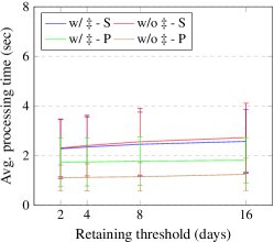
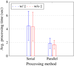
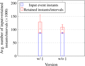
Experimental results The results of our evaluation are illustrated in Figure 3. We perform complex event processing with $ST=3h$, and $RT=\{2,4,8,16\}$ days. Figure 3 (left) shows the average processing time for each experiment. The results show that the addition of ${\ddagger}$ phenomena does not affect processing efficiency significantly, but also that Phenesthe+ is capable of producing detections in less than 2 seconds (multithreaded) when the data retaining threshold is set to 16 days. Note that the performance gain by running the multithreaded version of Phenesthe+ depends on the dependecies between phenomena and the computation of the processing order. For example, ${\mathit{fishing\_warning}}$ and ${\mathit{waiting\_time}}$ can be processed in parallel while ${\mathit{fishing\_warning}}$ and ${\mathit{suspicious\_trip}}$ cannot. In [23] we describe the computation of the processing order. With the addition of the new temporal phenomena, we limited the number of phenomena that can be processed in parallel. The results of Figure 3 (left) confirm this. We also perform complex event processing with $ST=24h$, and set $RT=\infty$ (i.e., keep non-redundant information forever)—recall that our dataset involves a 6 month period. Similar to the previous experiments we compare performance when Phenesthe+ is executed in parallel or serial manner, and with or without temporal phenomena marked with ${\ddagger}$ (see Table 1). Figure 3 (middle) shows the average processing time while Figure 3 (right) shows the average number of input entities plus retained instants/ intervals for each case. The results show, that in terms of processing time, performance is not significantly affected when including ${\ddagger}$ phenomena in both serial and parallel processing even when Phenesthe+ retains all information. In more detail, apart from the input events (on average 90K per temporal query) when we include ${\ddagger}$ phenomena the number of retained instants/intervals increases on average by 20K, therefore bringing the total number of input+retained entities up to 120K. Even in this setting Phenesthe+, produces detections in approximately 2 and 4 seconds (serial and parallel respectively).

Refer to caption
Refer to caption
Refer to caption
Figure 3: Experimental results. Average processing time per query with $ST=3h$ and $RT$ = $\{2,4,8,16\}$ days or $ST=24h$ and $RT$ = $\infty$ (left) and (middle) respectively. Average number of input plus retained instants/ intervals per query when $ST=24h$ and $RT=\infty$ (right).

7 Related work & Discussion

There are several very expressive temporal logics. The HS logic [17] is a very powerful logic for representing both instantaneous and durative temporal phenomena. When time is linear and the intervals homogeneous (therefore non overlapping) the HS logic is equally expressive with LTL but is exponentially more succinct [10]. In its original version, the HS logic does not make any assumptions on the nature of intervals. In this paper, we showed the TPhL- has equal expressive power to LTL, therefore concerning the linear HS variant studied in [10], TPhL- is equally expressive. It is well known, that the chop operator of Venema’s CDT logic [28] is inexpressible in the HS logic [21, 11]. TPhL supports the chop operator in the form of meets. While a formal expressiveness comparison of TPhL with the HS or CDT would be desirable, the omission of negation from $\Phi^{=}$ formulae makes this a challenging task.

Concerning our criteria for proper stream processors of TPhL, as mentioned earlier, their concepts are not entirely new. For example “correctness” has a similar notion with “soundness” in run-time verification [6] (i.e., the output should be correct with respect to the specification). Likewise, the “monotonicity” property as we have defined it, in run-time monitoring appears as the irrevocability property respectively for monitors [2]—a monitor that has the “irrevocability” property is unable to revoke the acceptance or the rejection of a trace. Finally, the “punctuality” property can be related to the “tightness” property of monitors [2], under which monitors are restricted to make a choice as soon as there is sufficient information available. In this work, we utilise the similar notions from run-time monitoring and verification for the task of complex event processing.

From a complex event processing perspective, LARS is a logic based framework for reasoning over streams [8]. While the language of LARS is expressible in LTL, the reverse direction does not hold, since LARS does not support ‘until’. A well known runtime monitoring system with point-based semantics is LOLA [14]. While LOLA does not allow durative phenomena, we saw in section 4 that formulae that hold on disjoint intervals can be expressed using point based modalities. It is not possible, however, to model formulae that hold on overlapping intervals. Furthermore, in the worst case LOLA requires memory equal to the size of the trace so far, which is not practical for large industrial applications such as maritime monitoring. In Phenesthe+ we allow the user to choose the retaining threshold. A complex event recognition framework is RTEC [5]. RTEC is a logic based formalism whereby events and fluents are expressed with a variant of the Event Calculus [19]. While there isn’t a formal study of the expressive power of the language of RTEC, its semantics suggest that it has at most equal expressive power with pure past LTL. Bauer et. al. [7], propose three valued semantics for monitoring LTL formulae. In our work, we also use three valued semantics, however for a more general case, as our language allows the representation of temporal phenomena that hold on overlapping intervals, which cannot be modeled in LTL. Team semantics for LTL [20] or HyperLTL [12] offer a promising direction towards the representation of concurrent temporal phenomena, however they are limited to a finite number of concurrent traces. In TPhL a dynamic temporal phenomenon may hold on possibly infinite overlapping intervals.

Closing, in this paper we presented TPhL and studied the expressive power of its different fragments. Specifically, we showed that TPhL${}^{-}_{o}$ has equal expressive power with pure past LTL while its extension, TPhL-, has equal expressive power with LTL. Concerning the complete logic TPhL, we showed that it is strictly less expressive than dyadic first-order logic. Moreover, we defined criteria for proper stream processors that use our language, and evaluated Phenesthe+, our stream processing implementation on real maritime data. Our results, show that Phenesthe+ is suitable for the task of maritime monitoring as it produces results in real-time. While the application of our experiment involved the maritime domain, Phenesthe+ is generic, and can be applied in other areas.

Regarding future work, we aim to study the expressive power of a theoretical variant of TPhL that includes negation on formulae of $\Phi^{=}$ in comparison with two-dimensional modal logics. Furthermore, as one of the main motivations for the creation of TPhL was facilitating writing temporal formulae, we plan to compare succinctness of TPhL- formulae with LTL formulae. Finally, we aim to apply Phenesthe+ for human activity monitoring in smart homes.

References

  • [1]
  • [2] Luca Aceto, Antonis Achilleos, Adrian Francalanza, Anna Ingólfsdóttir & Karoliina Lehtinen (2019): Adventures in Monitorability: From Branching to Linear Time and Back Again. Proc. ACM Program. Lang. 3(POPL), 10.1145/3290365.
  • [3] James F. Allen (1983): Maintaining knowledge about temporal intervals. Communications of the ACM 26(11), p. 832–843, 10.1145/182.358434.
  • [4] Darko Anicic, Paul Fodor, Sebastian Rudolph, Roland Stühmer, Nenad Stojanovic & Rudi Studer (2010): A Rule-Based Language for Complex Event Processing and Reasoning, p. 42–57. Lecture Notes in Computer Science 6333, Springer Berlin Heidelberg, 10.1007/978-3-642-15918-3_5.
  • [5] Alexander Artikis, Marek Sergot & Georgios Paliouras (2015): An Event Calculus for Event Recognition. IEEE Transactions on Knowledge and Data Engineering 27(4), pp. 895–908, 10.1109/TKDE.2014.2356476.
  • [6] Ezio Bartocci & Yliès Falcone, editors (2018): Lectures on Runtime Verification - Introductory and Advanced Topics. Lecture Notes in Computer Science 10457, Springer, 10.1007/978-3-319-75632-5.
  • [7] Andreas Bauer, Martin Leucker & Christian Schallhart (2011): Runtime Verification for LTL and TLTL. ACM Trans. Softw. Eng. Methodol. 20(4), 10.1145/2000799.2000800.
  • [8] Harald Beck, Minh Dao-Tran & Thomas Eiter (2018): LARS: A Logic-based framework for Analytic Reasoning over Streams. Artificial Intelligence 261, pp. 16–70, 10.1016/j.artint.2018.04.003.
  • [9] Michael H Bohlen, Renato Busatto & Christian S. Jensen (1998): Point-versus interval-based temporal data models. In: Proceedings 14th International Conference on Data Engineering, pp. 192–200, 10.1109/ICDE.1998.655777.
  • [10] Laura Bozzelli, Alberto Molinari, Angelo Montanari, Adriano Peron & Pietro Sala (2018): Interval vs. Point Temporal Logic Model Checking: An Expressiveness Comparison. ACM Trans. Comput. Logic 20(1), 10.1145/3281028.
  • [11] Davide Bresolin, Dario Della Monica, Valentin Goranko, Angelo Montanari & Guido Sciavicco (2008): Decidable and Undecidable Fragments of Halpern and Shoham’s Interval Temporal Logic: Towards a Complete Classification. In Iliano Cervesato, Helmut Veith & Andrei Voronkov, editors: Logic for Programming, Artificial Intelligence, and Reasoning, Springer Berlin Heidelberg, Berlin, Heidelberg, pp. 590–604, 10.1007/978-3-540-89439-1_41.
  • [12] Michael R. Clarkson, Bernd Finkbeiner, Masoud Koleini, Kristopher K. Micinski, Markus N. Rabe & César Sánchez (2014): Temporal Logics for Hyperproperties. In Martín Abadi & Steve Kremer, editors: Principles of Security and Trust - Third International Conference, POST 2014, Held as Part of the European Joint Conferences on Theory and Practice of Software, ETAPS 2014, Grenoble, France, April 5-13, 2014, Proceedings, Lecture Notes in Computer Science 8414, Springer, pp. 265–284, 10.1007/978-3-642-54792-8_15.
  • [13] Gianpaolo Cugola & Alessandro Margara (2010): TESLA: a formally defined event specification language. In: DEBS ’10, ACM Press, p. 50, 10.1145/1827418.1827427.
  • [14] Ben D’Angelo, Sriram Sankaranarayanan, Cesar Sanchez, Will Robinson, Bernd Finkbeiner, Henny B. Sipma, Sandeep Mehrotra & Zohar Manna (2005): LOLA: Runtime Monitoring of Synchronous Systems. In: Proceedings of the 12th International Symposium on Temporal Representation and Reasoning, TIME ’05, IEEE Computer Society, USA, p. 166–174, 10.1109/TIME.2005.26.
  • [15] Andreas Dohr, Christiane Engels & Andreas Behrend (2018): Algebraic Operators for Processing Sets of Temporal Intervals in Relational Databases. In Natasha Alechina, Kjetil Nørvåg & Wojciech Penczek, editors: 25th International Symposium on Temporal Representation and Reasoning (TIME 2018), Leibniz International Proceedings in Informatics (LIPIcs) 120, Schloss Dagstuhl–Leibniz-Zentrum fuer Informatik, Dagstuhl, Germany, pp. 11:1–11:16, 10.4230/LIPIcs.TIME.2018.11.
  • [16] Dov Gabbay, Amir Pnueli, Saharon Shelah & Jonathan Stavi (1980): On the Temporal Analysis of Fairness. In: Proceedings of the 7th ACM SIGPLAN-SIGACT Symposium on Principles of Programming Languages, POPL ’80, Association for Computing Machinery, New York, NY, USA, p. 163–173, 10.1145/567446.567462.
  • [17] Joseph Y. Halpern & Yoav Shoham (1991): A propositional modal logic of time intervals. Journal of the ACM 38(4), p. 935–962, 10.1145/115234.115351.
  • [18] Johan Anthony Wilem Kamp (1968): Tense Logic and the Theory of Linear Order. Ph.D. thesis, University of California, Los Angeles.
  • [19] Robert Kowalski & Marek Sergot (1986): A logic-based calculus of events. New Generation Computing 4(1), pp. 67–95, 10.1007/BF03037383.
  • [20] Andreas Krebs, Arne Meier, Jonni Virtema & Martin Zimmermann (2018): Team Semantics for the Specification and Verification of Hyperproperties. In Igor Potapov, Paul G. Spirakis & James Worrell, editors: 43rd International Symposium on Mathematical Foundations of Computer Science, MFCS 2018, August 27-31, 2018, Liverpool, UK, LIPIcs 117, Schloss Dagstuhl - Leibniz-Zentrum für Informatik, pp. 10:1–10:16, 10.4230/LIPIcs.MFCS.2018.10.
  • [21] Kamal Lodaya (2000): Sharpening the Undecidability of Interval Temporal Logic. In Jifeng He & Masahiko Sato, editors: Advances in Computing Science - ASIAN 2000, 6th Asian Computing Science Conference, Penang, Malaysia, November 25-27, 2000, Proceedings, Lecture Notes in Computer Science 1961, Springer, pp. 290–298, 10.1007/3-540-44464-5_21.
  • [22] Corto Mascle, Daniel Neider, Maximilian Schwenger, Paulo Tabuada, Alexander Weinert & Martin Zimmermann (2020): From LTL to RLTL Monitoring: Improved Monitorability through Robust Semantics. In: Proceedings of the 23rd International Conference on Hybrid Systems: Computation and Control, HSCC ’20, Association for Computing Machinery, New York, NY, USA, pp. 170–204, 10.1145/3365365.3382197.
  • [23] Manolis Pitsikalis, Alexei Lisitsa & Shan Luo (2021): Representation and Processing of Instantaneous and Durative Temporal Phenomena. In Emanuele De Angelis & Wim Vanhoof, editors: Logic-Based Program Synthesis and Transformation - 31st International Symposium, LOPSTR 2021, Tallinn, Estonia, September 7-8, 2021, Proceedings, Lecture Notes in Computer Science 13290, Springer, pp. 135–156, 10.1007/978-3-030-98869-2_8.
  • [24] Manolis Pitsikalis, Alexei Lisitsa, Patrick Totzke & Simon Lee (2022): Making Sense of Heterogeneous Maritime Data. In: 2022 23rd IEEE International Conference on Mobile Data Management (MDM), pp. 401–406, 10.1109/MDM55031.2022.00089.
  • [25] Amir Pnueli (1977): The temporal logic of programs. In: 18th Annual Symposium on Foundations of Computer Science (sfcs 1977), IEEE, Providence, RI, USA, p. 46–57, 10.1109/SFCS.1977.32.
  • [26] Alexander Rabinovich (2014): A Proof of Kamp’s theorem. Logical Methods in Computer Science Volume 10, Issue 1, 10.2168/LMCS-10(1:14)2014.
  • [27] Cyril Ray, Richard Dréo, Elena Camossi, Anne-Laure Jousselme & Clément Iphar (2019): Heterogeneous integrated dataset for Maritime Intelligence, surveillance, and reconnaissance. Data in Brief 25, p. 104141, 10.1016/j.dib.2019.104141.
  • [28] Yde Venema (1990): Expressiveness and completeness of an interval tense logic. Notre Dame Journal of Formal Logic 31(4), 10.1305/ndjfl/1093635589.
  • [29] Peter Øhrstrøm & Per Hasle (2006): Modern temporal logic: The philosophical background. In Dov M. Gabbay & John Woods, editors: Logic and the Modalities in the Twentieth Century, Handbook of the History of Logic 7, North-Holland, pp. 447–498, 10.1016/S1874-5857(06)80032-4.