Dynamic Manipulation of a Deformable Linear Object: Simulation and Learning

Abstract

We show that it is possible to learn an open-loop policy in simulation for the dynamic manipulation of a deformable linear object (DLO) – e.g., a rope, wire, or cable – that can be executed by a real robot without additional training. Our method is enabled by integrating an existing state-of-the-art DLO model (Discrete Elastic Rods) with MuJoCo, a robot simulator. We describe how this integration was done, check that validation results produced in simulation match what we expect from analysis of the physics, and apply policy optimization to train an open-loop policy from data collected only in simulation that uses a robot arm to fling a wire precisely between two obstacles. This policy achieves a success rate of 76.7% when executed by a real robot in hardware experiments without additional training on the real task.

I INTRODUCTION

The robotic manipulation of deformable linear objects (DLOs) is a popular area of research which finds many applications in the manufacturing and medical industry. Wire harness assembly is one such area which could benefit significantly from an automated assembly process. The final assembly process constitutes 70% of the production time while 90% of the process requires manual work [1]. Automation could be a means of cheaper and more efficient manufacturing in this area, especially when they are more widely used on safety-critical systems [2] and require stricter manufacturing processes which might not be suitable for less-experienced manual labour. An automated manufacturing process experiences failures which are more systematic, which are consequently easier to comprehend and anticipate. The objective of this work is to improve on learning the dynamic manipulation of DLOs, which could bring about future improvements in the automation of wire harness assembly. The flinging task is chosen to demonstrate this.

The main difficulties being faced in the manipulation of DLOs are their complex dynamics, the sensitivity of their movement to external and internal parameters, and the underactuated nature of their system [3]. To tackle this complex control task, forward sampling algorithms can be used. In recent years, reinforcement learning (RL) has also gained popularity as a solution to such problems. Both of these methods would benefit from an accurate simulator.

Dynamic manipulation of rigid objects could provide solutions to problems in which quasi-static methods are guaranteed to fail. The same could be the case when manipulating DLOs [4]. Other works on the dynamic manipulation of DLOs focus on learning a task by training an agent with real data to ensure that the training data obtained is accurate [5]. Works with training done in simulation did not focus on the accuracy of the simulation but was successful in bridging the sim-to-real gap by optimizing the actions of the system with a learnt implicit policy and adaptive action sampling to achieve its goal [6]. For both these methods, data has to be collected through real experiments.

Figure 1: Simulation environment with a wire and two obstacles in MuJoCo for the flinging task. The start (a) and a successful end (d) configuration are shown.

The first contribution of this paper is the implementation of an existing mathematical model of the Discrete Elastic Rods (DER) into MuJoCo*. The processes carried out before each time step in MuJoCo, and the simulator’s available functions, are taken into consideration when integrating the DER model into it. The implementation will be discussed more under Section III. This simulation will be useful for planning and learning accurate control tasks for wires. With it, we have designed a novel dynamic wire manipulation flinging task to demonstrate its use.

The second contribution is to show that the collection of real data for training can be reduced with the use of an accurate wire model when carrying out planning or learning. Real training data can be tedious to gather. With stiffness accurately modelled in the simulation, our method is able to successfully carry out the real task of flinging a wire, with a 76.7% success rate, using an agent that has only been trained in simulation.

II RELATED WORK

Simulation of DLOs have many uses apart from wire manipulation. DLOs have many different representations in simulation. These representations have been used in the study of polymers [7], musculoskeletal architectures [8], hair [9], and DNA [10]. Finite element models (FEMs) are a common way to represent DLOs. Many simulations make use of a mass-spring system. Despite their simplicity, an interpretation of the system parameters of these models as physical properties is lacking. To achieve the desired dynamic behavior could require substantial effort in tuning. The mass-spring system in MuJoCo is applied through ball joints between objects. The stiffness of the three rotational axes of a ball joint is represented by a single parameter. Consequently, the bending and twisting stiffness is represented by this stiffness parameter and cannot be adjusted independently. This limits its ability to accurately model DLOs. Position-based models [11] are widely used in computer animation for their visual plausibility but are not known for their physical accuracy. For the quasi-static manipulation of DLOs, their stable configurations are required where both the bending (curvature) and twisting (torsion) energy are at a local minimum. Minimal-energy curves have been successfully applied in both 2D [12] and 3D [13] to manipulate DLOs. The discrete elastic rod model [14] uses a similar concept of minimum energy to arrive at a stable configuration of the wire. In addition to bending and twisting, the Cosserat rod theory [15] [16] was able to include stretching and shearing to model elastic rods which have a wider array of applications. As wire stretching and shearing is relatively negligible for our application, the DER model will be used in this paper to reduce computational cost. More details will be discussed in Section III.

Manipulation of DLOs face many difficulties due to their complex dynamics and under-actuated nature. Past works have explored learning manipulation of ropes in a 2D space where the rope is placed flat against a table. In this way, moving a rope to pose proved successful through numerous learning techniques including learning from demonstrations [17] and learning from images [18]. Research has also been done to carry out more complex manipulation tasks on DLOs such as knot tying [19] by representing the DLO in its topological rather than geometrical state. In the 3D space, early works approached the manipulation problem by first sampling gripper pose, then using numerical simulation to approximate the wire configuration [13] [20]. Later, the set of all local solutions of a Kirchhoff elastic rod was shown to be a smooth manifold of finite dimension. As the smooth manifold can be parameterized by a single chart, manipulation planning was able to be carried out using sampling-based algorithms [21]. This was further brought to dual-arm manipulation of the rod [22] which was carried out using the path-connected property of the Kirchhoff elastic rod [23]. Another more specific manipulation task on DLOs uses a tactile sensor to trace a wire then insert it [24].

Dynamic manipulation of DLOs proves a greater challenge due to its high sensitivity to uncertainties. Iterative Residual Policy [6] was able accomplish tasks with complex dynamics by learning an implicit policy using delta dynamics and combining it with adaptive action sampling to optimize its actions to reach a goal. This technique was able to generalize to other scenarios better than alternative approaches. In Robots of the Lost Arc [5], three novel dynamic DLO manipulation tasks were introduced – vaulting, knocking, and weaving. A deep convolutional neural network along with quadratic programming has been successfully deployed in a pipeline to learn these tasks. When the learnt policy was deployed in real experiments, its results showed substantial improvement over a fixed and human-specified baseline. Their paper is what our work is largely inspired by. The simulation designed in their paper was used as a platform to experiment with the tasks and the learning algorithms before training is carried out with real experiments. By including an accurately modelled wire in simulation, our work will instead use the simulation to train a dynamic DLO manipulation policy. The intention of this is to reduce real training data required for learning. This will be explained further in Section IV.

III DYNAMIC WIRE SIMULATION

The method chosen in this paper for the simulation of a wire is using Discrete Elastic Rods (DER) [14]. This section will briefly introduce the DER model, along with some ideas behind it, followed by the structure of the simulation program.

III-A Discrete Elastic Rod

Modelling a wire continuously in simulation is infeasible due to its infinite dimensional property. DER theory splits a wire into discrete sections with which the wire dynamics can be analysed. The more discrete sections there are, the more closely the rod behaves like a real one. The DER paper differed from other approaches of its in terms of the kinematic description, where the twist of the material frame is represented by its angular deviation from the parallel-transported natural Bishop frame, and the dynamic treatment, where the material frame is treated as quasi-static while the centerline as dynamic. The explicit representation of the centerline makes it suitable for our simulation as it makes collision handling and rendering possible.

At each time step, the DER theory calculates the force on each node in the discrete rod as negative of the derivative of the energy with respect to the node position. This derivative can be obtained from the formulae of energy. Generally, the direction the force acts in is the direction in which expected node movement would most greatly decrease the sum of bending and twisting energy. This value is dependent on both the nodes positions and the twist in each discrete section. The formula is as follows. More details can be found in the original paper.

$$-\frac{dE(\Gamma)}{dx_{i}}=-\frac{\partial E(\Gamma)}{\partial x_{i}}-\sum_{j=0}^{n}\frac{\partial E(\Gamma)}{\partial\theta^{j}}\frac{\partial\theta^{j}}{\partial x_{i}}$$

III-B DER in MuJoCo

After calculating the centerline forces, constraint handling and integration of those forces will be carried out within MuJoCo [25]. Different physics simulators operate differently and have their own set of built-in functions. As such, they would require their own custom methods when integrating the DER model within them. Below details specifically the framework used to integrate the DER model into MuJoCo.

Modelling the Wire

Within the simulation, the wire is modelled as a continuous chain of discrete capsules (one of the base object types that can be simulated in MuJoCo) where the nodes are the joining points between these capsules. Each capsule is joined with the ’connect’ equality constraint in MuJoCo, which allows for rotational but not translational motions. These constraints will enforce the overall wire inextensibility constraint. As the capsules are free to rotate along the axis of their length without damping, an additional function is implemented in the simulation which resets the rotational velocity of all capsules at each time step. This is to ensure that the simulation does not become unstable from an unrestricted increase in the capsules’ rotational velocity.

Constraints-handling

In the original paper, an integration of the centerline using the forces calculated is applied, followed by a manifold projection method that is used to enforce constraint conditions, such as rod inextensibility. For this paper, we will make use of the constraint solver within MuJoCo to enforce constraints. The centerline forces calculated by the mathematical model is applied at each of the corresponding joints which connect the discrete bodies. A convex optimization problem is defined in the simulation where its global solution is the constraint forces. The solved constraint forces are then integrated to find the wire displacement.

III-C Implementation

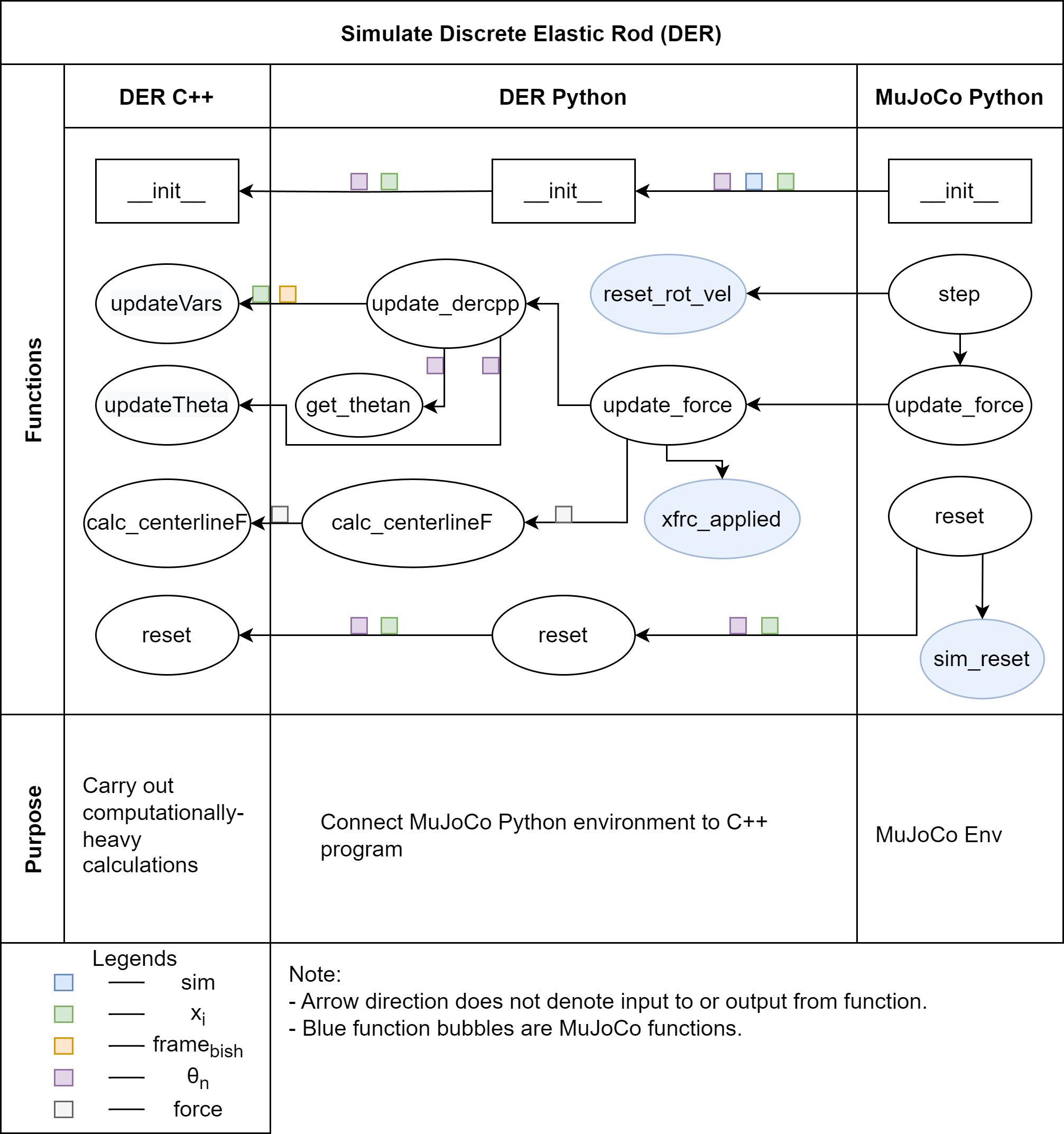
Figure 2: Overall simulation program structure

The MuJoCo simulation environment is created with mujoco-py. The structure of the overall program is reflected in Fig. 2. The program is first initialized along with the MuJoCo environment. At each time step, the update_force function is called which updates the program with the new twist angle, $\theta_{n}$, and the positions of the nodes, $x_{i}$. From these updated values, the program calculates the centerline forces on the wire. This force is applied to the nodes of the wire with the MuJoCo function, xfrc_applied, including these forces in the constraint equations of the simulator. The resultant movement of the wire is then calculated from the global solution of a formulated convex optimization problem solved by the MuJoCo simulator. The time step of the simulator has to be small enough such that no instability is caused when solving the optimization problem and to ensure that centerline forces are updated. Delayed calculation of the centerline forces due to large time steps might cause oscillations of the wire similar to a control system with its control frequency set too low. A suitable time step which balances the trade-off between the stability of the simulation and its computation time is found to be around 0.002 seconds. Open-source code of the wire model in MuJoCo is available on GitHub: https://github.com/qj25/der_mujoco.git.

Simulation Speeds

For both types of simulations, with and without DER calculations (WD and WOD, respectively), the wire is modelled as a continuous chain of discrete capsules, connected with the MuJoCo connect constraint, as described above. The connect constraint does not have bending nor twisting stiffness and only serves to keep the discrete capsules linked. WD includes the DER functions that calculate and exert the centerline forces which simulate wire stiffness, while WOD does not. These functions increase the computation time required. The computation times are shown in Table  I. The speed tests are a measure of the real computation time taken (average of 300 environment runs) to simulate one simulation time step (0.002s) with varying numbers of discrete rod sections, with and without the DER force calculations. As can be seen, the percentage increase in time taken decreases when more sections are simulated. This means that the number of sections can be increased without concerns that the time taken for stiffness calculations will increase exponentially.

Table I: Computation time to run one simulation time step (0.002s)

No. of Discrete Sections, $n$	Only Simulating Discrete Connected Sections in MuJoCo (s)	With additional DER calculations (ms)	Increase in time taken (%)
20	0.320	0.362	12.93
30	0.555	0.597	7.78
40	0.712	0.758	6.51
50	0.967	1.015	4.92
60	1.262	1.319	4.53

III-D Validation

To ensure that our simulation model of a straight isotropic wire is accurate, some validation tests from [14] are carried out here. The referenced work compares some testing results with available analytical solutions. Using the localized helical buckling and Michell’s buckling instability tests, consistency with those results will validate our simulation model.

Localized helical buckling

For a straight isotropic rod, localized helical buckling occurs when a twist is introduced to one rod end and the rods ends are brought towards each other, quasi-statically. The solution to this buckling can be described by an analytical solution. Our model is shown to converge to this analytical solution as the number of discrete section increases. A plot of the envelope of the helix, $f(\varphi)$ against the dimensionless arc length, $s/s*$, is shown in Fig. 3, where $\varphi=cos^{-1}(\mathbf{t}.\mathbf{e}_{x})$ is the angular deviation of the tangent away from the axis passing through the rod end points. $s$ is the rod arc length. The helix envelope can be simplified as $f(\varphi)=\frac{cos(\varphi)-cos(\varphi_{0})}{1-cos(\varphi_{0})}$ [26], where $s/s*=(\frac{\beta m}{2\alpha}\sqrt{\frac{1-cos(\varphi_{0})}{1+cos(\varphi_{0})}})s$, and the maximal angular deviation of the wire from the tangent can be calculated as $\varphi_{0}=max_{s}\varphi(s)$. $\alpha$ and $\beta$ are the bending and twisting stiffness, respectively. $m$ is the overall twist over the rod length. The graph is shown to converge towards the analytical solution as more discrete sections are used to represent the rod.

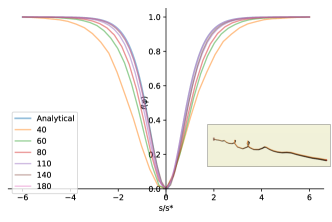
Figure 3: Localized Helical Buckling Test on a straight isotropic rod. A twist of 27 turns is imposed on one end of the rod. The rod has properties as follows: $L=9.29$, $\alpha=1.345$, $\beta=0.789$. The ends are brought closer together by 0.3 units which causes helical buckling on the rod. The test is carried out with different values of $n$ as shown in the legends. It can be seen that the plot converges to the analytical values as $n$ increases.

Table II: Validation Results for Localized Helical Buckling Test

Number of Discrete Sections, $n$	Average Error (unit per data point)
40	0.020736
60	0.008613
80	0.004083
110	0.001716
140	0.000782
180	0.000296

Michell’s Instability

Connecting the ends of a straight isotropic rod results in a loop being formed. This loop lies in a single plane. Michell’s instability occurs when one end is twisted along the tangent axis of the rod while the other is kept still. As this twist angle increases buckling of the loop occurs, causing the loop to fall out of the original plane. This phenomenon shows the coupling between the rod twist and its equilibrium configuration. Buckling occurs at a critical twist angle which can be determined analytically as $\theta^{n}_{c}=2\pi\sqrt{3}/(\beta/\alpha)$ when the loop radius, $R=1$ [27] [28]. Fig. 4 shows the graph of critical buckling angle against $\beta/\alpha$ that was obtained by testing our simulation model. It is shown that our model’s results are similar to that of the results obtained analytically with a maximum deviation of $1.68\%$ from the analytical plot when $\beta/\alpha=0.5$.

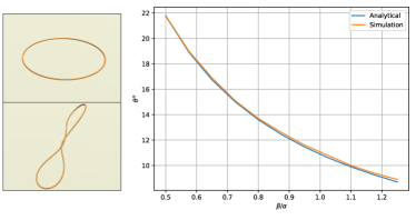
Figure 4: Michell’s Instability Test on a straight isotropic rod with ends connected to form an elastic ring. One end is twisted a certain amount until a critical value is reached whereby the circular shape buckles into a non-planar shape in the presence of small external disturbances. $\alpha=1$ and number of discrete rods, $n=50$, while $\beta$ is varied to achieve different values of $\beta/\alpha$ for which the critical twist, $\theta^{n}$ depends.

IV WIRE MANIPULATION

This section will focus on the dynamic manipulation of DLOs with robot arms. More specifically, how flinging, a complex dynamic task, can be accomplished with policy optimization in the environment created. In the environment, one end of the wire is fixed to a point in the world space and the other is attached to the end-effector of a 7R Panda robot arm.

IV-A Flinging Task

To demonstrate the usefulness of this simulation environment in robotics planning and learning for the manipulation of DLOs, we will carry out a single step policy optimization on the problem of flinging a 2-meter wire between two obstacles on a table. The task can not be easily accomplished with quasi-static manipulations due to the proximity of the wire ends and the restricted movement of the robot arm. Because of the complex dynamics of a wire and the under-actuated nature of manipulating one, classical methods have shown issues of being resolution incomplete. Therefore, optimization on dynamic actions is chosen as our solution. A render of the environment is shown in Fig. 1. Flinging too softly will not allow the wire to go over either obstacles, while flinging too hard will cause the wire to go over both obstacles. The movable end of the wire is assumed to be firmly grasped by the robot arm end-effector. The task is successful if, at the end of the robot arm motion, the wire comes to rest between the two obstacles.

IV-A1 Policy Optimization

To learn the task, we make use of the stochastic policy optimization algorithm within Proximal Policy Optimization (PPO) [29]. Our simulation environment is designed with only a single step per episode. It provides its initial state as an input to the algorithm. The algorithm then outputs an action vector back to the environment to run. Depending on the results of that run, the policy is updated. Instead of collecting a large random dataset for training, this method updates its policy based on the results returned from taking the stochastic actions decided by the policy itself. Essentially, this implementation is a single step RL algorithm [30] which holds the benefit that the resulting environment structure allows for other RL algorithms to be easily applied when designing similar simulation experiments which require closed-loop control.

The PPO algorithm used for policy optimization is provided by the Stable-Baselines3 [31] package and trained on a gym [32] environment of our simulation. The action space output, $U$, of the learning algorithm is a custom parameterized dynamic trajectory. In [5], the dynamic manipulation tasks were successfully carried out with a parameterized trajectory created, using a quadratic programming solver, from an apex point and fixed start and end points. Our paper uses multiple Cartesian sample points within the restricted robot end-effector operational space, along with splines, to obtain the final joint trajectory. This is done with the intention of exposing the robot arm to a larger variety of movements while keeping the size of the action space reasonable. These sample points are restricted to $y$ and $z$ axis translational and $y$ axis rotational pose differences from the initial start position of the robot end-effector. A total of 3 such sample points are taken, after which analytical inverse kinematic [33] is carried out to determine the joint position at these sampled points. With a total of 4 sets of joint positions (3 sampled + 1 start position), a B-spline interpolation [34] is done on each of the 7 joints. Following that, the joint trajectory obtained is fed into a joint position controller which commands the robot arm to carry out the motion. The input to the algorithm is the bending and twisting modulus of the wire, $\alpha$ and $\beta$, respectively. $d_{err}$ is calculated as the closest distance between the position of the wire and the center of the top of the two obstacles. If the wire is between the obstacles, $d_{err}=0$. This error value is used to calculate the return or reward function. The environment terminates after 75 controller command steps which is enough for the wire to settle into a sufficiently stable state.

The reward function, $r$ is the negative of the minimum $d_{err}$ achieved throughout the flinging. The smaller each $d_{err}$ is, the closer the reward function is to 0. In addition, a reward of +10 is given when the task is successfully carried out ($success_{true/false}=10$, else $success_{true/false}=0$ if task fails).

The overall formula is as follows:

$$r=max(-min(d_{err}),10*success_{true/false})$$

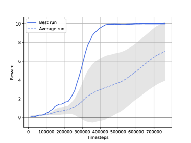
Figure 5: Plot of mean episode reward against training time steps. Training is done with a wire simulated using 30 discrete sections. The dashed line shows the average rewards while the shaded region represents the mean standard deviation during training. The solid line shows the agent which was able to achieve the highest reward with the least time steps.

The environment is trained with 750,000 time steps total. Training is done on a simulation environment which use 30 simulated rod sections. Results for the optimization are shown in Fig. 5. The reward increases with training time steps and approaches its maximum value (+10). Some of the policies are observed to start improving later, creating a high variance for the overall training.

V REAL EXPERIMENT

Real experiments for the flinging task are carried out to determine if the Panda robot arm is able to accomplish it and reflect the results obtained from training in simulation. Following that, wire positions for the real experiment will be obtained. This will be done using a stereo vision camera to capture the experiment, specifically identifying the wire’s features of interest and filtering out other features. This information will be plotted and compared with the wire positions captured in the MuJoCo environment to determine the accuracy of the model in simulating the real flinging experiment.

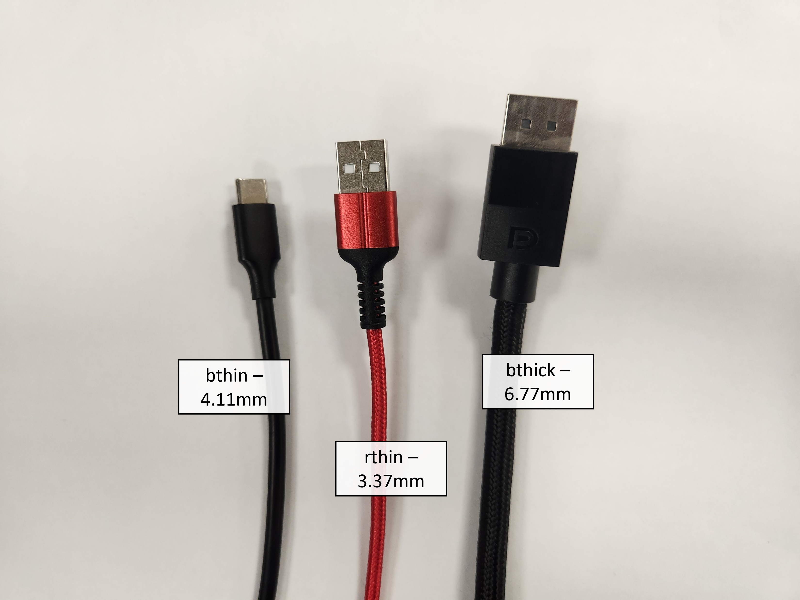
Figure 6: The three wires of varying thickness and material used for the flinging task.

For the real experiments, we will use the policy which was able to arrive at the maximum reward with the least time steps. Three different wires (Fig. 6) with varying thickness and material properties were used. The experiment was repeated a total of 30 times for each wire using the policy trained. The success rates are 76.6% (23/30 runs) for bthin, 10.0% (3/30 runs) for rthin, and 83.3% (25/30 runs) for bthick. A possible reason bthin and bthick be show more consistent results is that they are more uniformly straight in their neutral position as compared to rthin. Another possible reason is that the wires modelled in simulation have parameters which more closely match the two black wires. All of the failures of rthin are caused by the robot arm flinging the wire over both obstacles instead of just one. The black wires experienced both under-flinging and over-flinging in their failure cases.

V-A Experiment Setup

The experiment is set up as shown in Fig. 7. Placement of each object follows the simulated environment. Only two meters of each wire will be used as per the simulated environment. White tapes are placed at 20 cm intervals for ease of feature detection. Experiments are reset to the same position each time as shown in Fig. 7 (a). The stereo camera used is the Intel Realsense D435i, which captures the left and right monochrome frames and a color frame. Each of the cameras runs at a rate of 30 frames per second. The D435i cameras use a global shutter which are suitable for capturing high speed objects without distortion. The shutter speed has to be set relatively high to ensure that there is minimal blur for ease of feature detection.

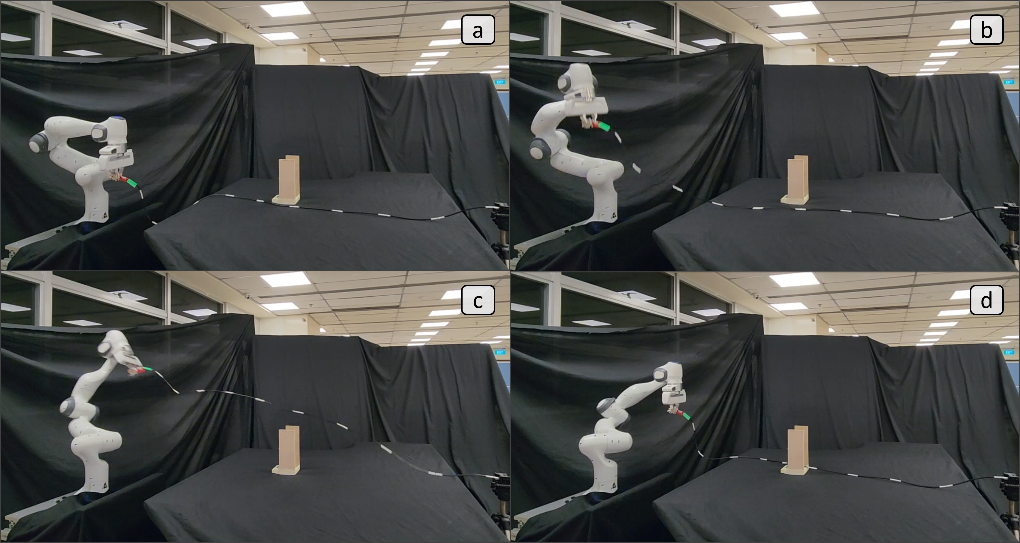
Figure 7: Flinging Experiment Setup along with an example of a successful flinging motion carried out by the Panda Robot Arm (a to d).

V-B Stereo Vision

As the feature detection for the Intel Realsense software is designed for general use, it is not able to reliably detect the relatively thin wires in the images. Using the OpenCV Library [35], a stereo vision program was written which detects the features in the left and right images, match them, filter out unnecessary points, and connect the remaining points into a continuous wire using splines. This is done on the experiment conducted with the rthin wire. The results are as shown in Fig. 8.

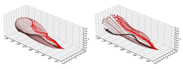
Figure 8: Comparison of Real Experiment Results (right) using stereo vision with the Simulation (left). The colors of the plot shows the time of the fling at which the frame was captured, i.e. black (start) to red (end).

The stereo vision results might contain inaccuracies due to the limited depth resolution available from the 1280x720p monochrome images. In addition, inaccuracies might arise from the splines used to connect marker points as they are just an approximation of the wire shape. The splines interpolate between the identified points and could results in a loss of feature, especially in areas where the curvature of the wire is high such as the end position of the wire. Despite this, the general shape of the real wire movement is similar to that obtained in simulation.

VI CONCLUSIONS

To accurately model a wire, the existing model of a DER has been integrated into MuJoCo. Validation results show that the simulator performs similarly to the model in the original DER paper [14]. Policy optimization was employed to learn a dynamic task on the simulator. Its reliability was shown in the results of the real experiments, where the task was executed with a 76.7% success rate, without further training on real data. We are able to compare the difference between the wire movement in the real and simulated experiments. Although the general movement of the wire is observed to be similar, more can be done to improve the accuracy of the simulation such as accurately modelling friction of the wire and identifying the right stiffness parameters to use.

VI-A Limitations and Future Work

One of the limitations is that the output trajectory from the policy is only a guide for the robot arm to follow due to the nature of the joint trajectory controller and how the expected trajectory is deployed. The actual trajectory the robot takes in the simulator is slightly different. As such, the controller of the real robot would have to be tuned precisely to ensure it performs similarly to the one in the simulator.

Future work will be done on carrying out parameter identification of the wire. Another option is to design the experiment in such a way that it is robust to parameter uncertainties. The designed flinging task is an open-loop problem. In future, the environment can be designed and employed to solve more complex problems which require closed-loop control.

References

- [1] H. G. Nguyen, M. Kuhn, and J. Franke, “Manufacturing automation for automotive wiring harnesses,” Procedia CIRP, vol. 97, pp. 379–384, 2021.
- [2] M. Kuhn, H. G. Nguyen, H. Otten, and J. Franke, “Blockchain enabled traceability–securing process quality in manufacturing chains in the age of autonomous driving,” in 2018 IEEE International Conference on Technology Management, Operations and Decisions (ICTMOD). IEEE, 2018, pp. 131–136.
- [3] J. Zhu, A. Cherubini, C. Dune, D. Navarro-Alarcon, F. Alambeigi, D. Berenson, F. Ficuciello, K. Harada, X. Li, J. Pan et al., “Challenges and outlook in robotic manipulation of deformable objects,” arXiv preprint arXiv:2105.01767, 2021.
- [4] Q.-C. Pham, S. Caron, P. Lertkultanon, and Y. Nakamura, “Admissible velocity propagation: Beyond quasi-static path planning for high-dimensional robots,” The International Journal of Robotics Research, vol. 36, no. 1, pp. 44–67, 2017.
- [5] H. Zhang, J. Ichnowski, D. Seita, J. Wang, H. Huang, and K. Goldberg, “Robots of the lost arc: Self-supervised learning to dynamically manipulate fixed-endpoint cables,” in 2021 IEEE International Conference on Robotics and Automation (ICRA). IEEE, 2021, pp. 4560–4567.
- [6] C. Chi, B. Burchfiel, E. Cousineau, S. Feng, and S. Song, “Iterative residual policy: for goal-conditioned dynamic manipulation of deformable objects,” arXiv preprint arXiv:2203.00663, 2022.
- [7] P. A. Wiggins, R. Phillips, and P. C. Nelson, “Exact theory of kinkable elastic polymers,” Physical Review E, vol. 71, no. 2, p. 021909, 2005.
- [8] X. Zhang, F. K. Chan, T. Parthasarathy, and M. Gazzola, “Modeling and simulation of complex dynamic musculoskeletal architectures,” Nature communications, vol. 10, no. 1, pp. 1–12, 2019.
- [9] F. Bertails, B. Audoly, M.-P. Cani, B. Querleux, F. Leroy, and J.-L. Lévêque, “Super-helices for predicting the dynamics of natural hair,” ACM Transactions on Graphics (TOG), vol. 25, no. 3, pp. 1180–1187, 2006.
- [10] Y. V. Sereda and T. C. Bishop, “Evaluation of elastic rod models with long range interactions for predicting nucleosome stability,” Journal of Biomolecular Structure and Dynamics, vol. 27, no. 6, pp. 867–887, 2010.
- [11] N. Umetani, R. Schmidt, and J. Stam, “Position-based elastic rods,” in ACM SIGGRAPH 2014 Talks, 2014, pp. 1–1.
- [12] E. Jou and W. Han, “Minimal-energy splines with various end constraints,” in Curve and surface design. SIAM, 1992, pp. 23–40.
- [13] M. Moll and L. E. Kavraki, “Path planning for deformable linear objects,” IEEE Transactions on Robotics, vol. 22, no. 4, pp. 625–636, 2006.
- [14] M. Bergou, M. Wardetzky, S. Robinson, B. Audoly, and E. Grinspun, “Discrete elastic rods,” in ACM SIGGRAPH 2008 papers, 2008, pp. 1–12.
- [15] E. Cosserat, Théorie des corps déformables. Librairie Scientifique A. Hermann et Fils, 1909.
- [16] J. Spillmann and M. Teschner, “Corde: Cosserat rod elements for the dynamic simulation of one-dimensional elastic objects,” in Proceedings of the 2007 ACM SIGGRAPH/Eurographics symposium on Computer animation, 2007, pp. 63–72.
- [17] A. Nair, D. Chen, P. Agrawal, P. Isola, P. Abbeel, J. Malik, and S. Levine, “Combining self-supervised learning and imitation for vision-based rope manipulation,” in 2017 IEEE international conference on robotics and automation (ICRA). IEEE, 2017, pp. 2146–2153.
- [18] A. Wang, T. Kurutach, K. Liu, P. Abbeel, and A. Tamar, “Learning robotic manipulation through visual planning and acting,” arXiv preprint arXiv:1905.04411, 2019.
- [19] M. Saha and P. Isto, “Manipulation planning for deformable linear objects,” IEEE Transactions on Robotics, vol. 23, no. 6, pp. 1141–1150, 2007.
- [20] F. Lamiraux and L. E. Kavraki, “Planning paths for elastic objects under manipulation constraints,” The International Journal of Robotics Research, vol. 20, no. 3, pp. 188–208, 2001.
- [21] T. Bretl and Z. McCarthy, “Quasi-static manipulation of a kirchhoff elastic rod based on a geometric analysis of equilibrium configurations,” The International Journal of Robotics Research, vol. 33, no. 1, pp. 48–68, 2014.
- [22] A. Sintov, S. Macenski, A. Borum, and T. Bretl, “Motion planning for dual-arm manipulation of elastic rods,” IEEE Robotics and Automation Letters, vol. 5, no. 4, pp. 6065–6072, 2020.
- [23] A. Borum and T. Bretl, “The free configuration space of a kirchhoff elastic rod is path-connected,” in 2015 IEEE International Conference on Robotics and Automation (ICRA). IEEE, 2015, pp. 2958–2964.
- [24] Y. She, S. Wang, S. Dong, N. Sunil, A. Rodriguez, and E. Adelson, “Cable manipulation with a tactile-reactive gripper,” The International Journal of Robotics Research, vol. 40, no. 12-14, pp. 1385–1401, 2021.
- [25] E. Todorov, T. Erez, and Y. Tassa, “Mujoco: A physics engine for model-based control,” in 2012 IEEE/RSJ international conference on intelligent robots and systems. IEEE, 2012, pp. 5026–5033.
- [26] G. Van der Heijden and J. Thompson, “Helical and localised buckling in twisted rods: a unified analysis of the symmetric case,” Nonlinear dynamics, vol. 21, no. 1, pp. 71–99, 2000.
- [27] J. Michell, “On the stability of a bent and twisted wire,” Messenger Math, vol. 11, pp. 181–184, 1889.
- [28] A. Goriely, “Twisted elastic rings and the rediscoveries of michell’s instability,” Journal of Elasticity, vol. 84, no. 3, pp. 281–299, 2006.
- [29] J. Schulman, F. Wolski, P. Dhariwal, A. Radford, and O. Klimov, “Proximal policy optimization algorithms,” arXiv preprint arXiv:1707.06347, 2017.
- [30] H. Ghraieb, J. Viquerat, A. Larcher, P. Meliga, and E. Hachem, “Single-step deep reinforcement learning for open-loop control of laminar and turbulent flows,” Physical Review Fluids, vol. 6, no. 5, p. 053902, 2021.
- [31] A. Raffin, A. Hill, M. Ernestus, A. Gleave, A. Kanervisto, and N. Dormann, “Stable baselines3,” 2019.
- [32] G. Brockman, V. Cheung, L. Pettersson, J. Schneider, J. Schulman, J. Tang, and W. Zaremba, “Openai gym,” arXiv preprint arXiv:1606.01540, 2016.
- [33] Y. He and S. Liu, “Analytical inverse kinematics for franka emika panda–a geometrical solver for 7-dof manipulators with unconventional design,” in 2021 9th International Conference on Control, Mechatronics and Automation (ICCMA). IEEE, 2021, pp. 194–199.
- [34] C. De Boor and C. De Boor, A practical guide to splines. springer-verlag New York, 1978, vol. 27.
- [35] G. Bradski and A. Kaehler, Learning OpenCV: Computer vision with the OpenCV library. ” O’Reilly Media, Inc.”, 2008.