DataInf: Efficiently Estimating Data Influence in LoRA-tuned LLMs and Diffusion Models

Abstract

Quantifying the impact of training data points is crucial for understanding the outputs of machine learning models and for improving the transparency of the AI pipeline. The influence function is a principled and popular data attribution method, but its computational cost often makes it challenging to use. This issue becomes more pronounced in the setting of large language models and text-to-image models. In this work, we propose DataInf, an efficient influence approximation method that is practical for large-scale generative AI models. Leveraging an easy-to-compute closed-form expression, DataInf outperforms existing influence computation algorithms in terms of computational and memory efficiency. Our theoretical analysis shows that DataInf is particularly well-suited for parameter-efficient fine-tuning techniques such as LoRA. Through systematic empirical evaluations, we show that DataInf accurately approximates influence scores and is orders of magnitude faster than existing methods. In applications to RoBERTa-large, Llama-2-13B-chat, and stable-diffusion-v1.5 models, DataInf effectively identifies the most influential fine-tuning examples better than other approximate influence scores. Moreover, it can help to identify which data points are mislabeled.

1 Introduction

Modern large language models (LLMs) and text-to-image models have demonstrated remarkable abilities in generating human-like texts and photorealistic images, leading to diverse real-world applications such as translation, dialogue systems, and image editing [1, 2, 3]. Nevertheless, even state-of-the-art models do generate factually incorrect predictions or even biased outputs [4, 5, 6], often as a result of issues in the training data. This highlights the need for principled and systematic methods to quantify the impact of specific training data points. The influence function provides a rigorous framework for evaluating the impact of each training data point on model predictions [7, 8]. Its efficacy has been demonstrated across various downstream machine learning tasks: mislabeled data detection [9], best subset selection [10, 11], model interpretation [12, 13, 14], and investigation of model biases [15, 16].

While the influence function has shown promising results, its application in real-world scenarios poses practical challenges because of its expensive computational costs. Calculating the influence function requires the computation of the inverse Hessian matrix, which involves intensive computation. Previous studies have attempted to reduce this burden; however, most existing methods still require an iterative algorithm [17, 18], multiple eigenvalue decompositions [19] or the training of numerous models [10] to obtain accurate influence estimates. It has therefore been very challenging to compute the influence function for large models such as LLMs [20, 21, 22] and diffusion models [23, 24, 2].

Our contributions

We propose DataInf, a computationally efficient influence approximation method that can be easily applied to large-scale machine learning models. DataInf is based on an easy-to-compute closed-form expression, leading to better computational and memory complexities than existing state-of-the-art influence computation algorithms. Our approximation error analysis suggests that DataInf is especially effective when it is applied to parameter-efficient fine-tuned models to estimate the influence of fine-tuning data. We evaluate the practical efficacy of DataInf through three sets of experiments: approximation error analysis, mislabeled data detection, and influential data identification. Our empirical results demonstrate that DataInf is faster and more effective in retrieving the most (or the least) influential training data points than existing algorithms. We apply DataInf to the RoBERTa, Llama-2-13B-chat, and stable-diffusion-v1.5 models, demonstrating that it is easily applicable to LLMs and large-scale diffusion models.

2 Preliminaries

We denote an input space and a label space by $\mathcal{X}$ and $\mathcal{Y}$, respectively. We denote a training dataset by $\mathcal{D}=\{(x_{i},y_{i})\}_{i=1}^{n}$ where $x_{i}\in\mathcal{X}$ and $y_{i}\in\mathcal{Y}$ are an input and a label of the $i$-th datum. We consider the empirical risk minimization framework: For a loss function $\ell\mathrel{\mathop{\mathchar 58\relax}}\mathcal{Y}\times\mathcal{Y}\to\mathbb{R}$ and a parameter space $\Theta$, the empirical risk minimizer is defined as follows:

$$\theta^{*}\mathrel{\mathop{\mathchar 58\relax}}=\mathrm{argmin}_{\theta\in\Theta}\frac{1}{n}\sum_{i=1}^{n}\ell(y_{i},f_{\theta}(x_{i})),$$

where $f_{\theta}\mathrel{\mathop{\mathchar 58\relax}}\mathcal{X}\to\mathcal{Y}$ is a model parametrized with $\theta\in\Theta$. We set $[m]\mathrel{\mathop{\mathchar 58\relax}}=\{1,\dots,m\}$ for $m\in\mathbb{N}$. For $i\in[n]$ and a vector $\eta$, we denote a gradient of the $i$-th loss with respect to $\eta$ by $\nabla_{\eta}\ell_{i}\mathrel{\mathop{\mathchar 58\relax}}=\nabla_{\eta}\ell(y_{i},f_{\theta}(x_{i}))$.

2.1 Influence Function

The influence function assesses the impact of individual training data points on parameter estimation [7, 8, 25]. It captures how fast parameter estimates change when a particular data point is up-weighted. To be more specific, for $k\in[n]$ and $\varepsilon\in\mathbb{R}$, we consider the following $\varepsilon$-weighted risk minimization problem:

$$\theta^{(k)}(\varepsilon)\mathrel{\mathop{\mathchar 58\relax}}=\mathrm{argmin}_{\theta\in\Theta}\frac{1}{n}\sum_{i=1}^{n}\ell(y_{i},f_{\theta}(x_{i}))+\varepsilon\ell(y_{k},f_{\theta}(x_{k})).$$

When a loss function $\ell(y,f_{\theta}(x))$ is twice-differentiable and strongly convex in $\theta$ for all $(x,y)\in\mathcal{X}\times\mathcal{Y}$, the empirical risk minimizer $\theta^{*}$ is well-defined, and the influence of the $k$-th data point $(x_{k},y_{k})\in\mathcal{D}$ on the empirical risk minimizer $\theta^{*}$ is defined as the derivative of $\theta^{(k)}(\varepsilon)$ at $\varepsilon=0$ [7, 26].

$$\mathcal{I}_{\theta^{*}}(x_{k},y_{k})\mathrel{\mathop{\mathchar 58\relax}}=\frac{d\theta^{(k)}}{d\varepsilon}\Big{\rvert}_{\varepsilon=0}=-H(\theta^{*})^{-1}\nabla_{\theta}\ell_{k},$$

where $H(\theta)\mathrel{\mathop{\mathchar 58\relax}}=\nabla_{\theta}^{2}\left(n^{-1}\sum_{i=1}^{n}\ell(y_{i},f_{\theta}(x_{i}))\right)$ is the Hessian of the empirical loss.

In machine learning problems, the influence function $\mathcal{I}_{\theta^{*}}(x_{k},y_{k})$ on the empirical risk minimizer $\theta^{*}$ is extended to the influence function on a prediction loss [9]. For a validation dataset $\mathcal{D}^{\mathrm{(val)}}\mathrel{\mathop{\mathchar 58\relax}}=\{(x_{i}^{\mathrm{(val)}},y_{i}^{\mathrm{(val)}})\}_{i=1}^{m}$, the influence of $(x_{k},y_{k})$ on the validation loss is defined as:

$$\mathcal{I}(x_{k},y_{k}) \mathrel{\mathop{\mathchar 58\relax}}=\left(\frac{1}{m}\sum_{i=1}^{m}\nabla_{\theta}\ell(y_{i}^{\mathrm{(val)}},f_{\theta}(x_{i}^{\mathrm{(val)}}))\rvert_{\theta=\theta^{*}}\right)^{T}\mathcal{I}_{\theta^{*}}(x_{k},y_{k}).$$

The influence function $\mathcal{I}(x_{k},y_{k})$ provides an intuitive interpretation of how one data point affects the validation loss. When $\mathcal{I}(x_{k},y_{k})$ is a large positive (resp. negative) value, the validation loss would increase (resp. decrease) as the data point $(x_{k},y_{k})$ is up-weighted because $\mathcal{I}(x_{k},y_{k})$ is defined as a gradient of the validation loss. In other words, the influence function intuitively represents whether $(x_{k},y_{k})$ is beneficial or detrimental to the prediction loss.

While the influence function is established on a rigorous statistical framework, its computation often poses practical challenges due to the second-order gradients in $H(\theta^{*})$. Calculating the second-order gradient is computationally intensive in general, but it can be achieved with the first-order gradient when the loss function is a negative log-likelihood function [27]. To elaborate, suppose $\ell(y,f_{\theta}(x))=-\log p(y\mid f_{\theta}(x))$ for all $(x,y)\in\mathcal{X}\times\mathcal{Y}$ and $\theta\in\Theta$ where $p(y\mid f_{\theta}(x))$ is a probability density function of $(x,y)$ at $\theta$. Bartlett’s second identity implies that

$$\mathbb{E}\left[\nabla_{\theta}^{2}\ell(Y,f_{\theta}(X))\right] =\mathbb{E}\left[\nabla_{\theta}\ell(Y,f_{\theta}(X))\left(\nabla_{\theta}\ell(Y,f_{\theta}(X))\right)^{T}\right],$$

where the expectation is over the distribution $p(Y\mid f_{\theta}(X))$. That is, the Hessian $H(\theta^{*})$ can be replaced with the second moment of the first-order gradients $G(\theta^{*})\mathrel{\mathop{\mathchar 58\relax}}=n^{-1}\sum_{i=1}^{n}\nabla_{\theta}\ell_{i}\nabla_{\theta}\ell_{i}^{T}$. This yields the following formula for the influence function:

$$-\left(\frac{1}{m}\sum_{i=1}^{m}\nabla_{\theta}\ell(y_{i}^{\mathrm{(val)}},f_{\theta}(x_{i}^{\mathrm{(val)}}))\rvert_{\theta=\theta^{*}}\right)^{T}G(\theta^{*})^{-1}\nabla_{\theta}\ell_{k}.$$ (1)

2.2 Influence function for deep neural network models

The influence function in (1) can be computed with only the first-order gradients; however, there are practical challenges when $f_{\theta}$ is a deep neural network model [28, 29]. First, when the dimension of $\theta$ exceeds the sample size $n$, which is common in many modern machine learning problems, $G(\theta)$ is not invertible because the rank of $G(\theta)$ is at most $n$. Second, the size of $G(\theta)$ is too large to compute, making its computation infeasible.

To address the first issue, the “damping Hessian” approach is used in which a small positive number is added to diagonal elements of $G(\theta)$ and make it positive definite [17]. As for the second issue, $G(\theta)$ is replaced with its block diagonal matrix, where each block corresponds to a layer of a deep neural network model. To be more specific, suppose $f_{\theta}$ can be expressed as a composition function $f_{\theta}(x)=f_{\theta_{L}}\circ\cdots\circ f_{\theta_{1}}(x)$ where for $l\in[L]$, we denote a vectorized notation of weights and biases in the $l$-th layer by $\theta_{l}\in\mathbb{R}^{d_{l}}$ for some $d_{l}\in\mathbb{N}$. Then, the $l$-th diagonal block of $G(\theta)$ can be expressed as $G_{l}(\theta)\mathrel{\mathop{\mathchar 58\relax}}=n^{-1}\sum_{i=1}^{n}\nabla_{\theta_{l}}\ell_{i}\nabla_{\theta_{l}}\ell_{i}^{T}$, and $G(\theta)$ is replaced with $\mathrm{diag}(G_{1}(\theta),\dots,G_{L}(\theta))$ [14]. Combining these approaches gives the following influence function:

$$-\sum_{l=1}^{L}v_{l}^{T}\left(G_{l}(\theta^{*})+\lambda_{l}I_{d_{l}}\right)^{-1}\nabla_{\theta_{l}}\ell_{k}$$ (2)

where $v_{l}\mathrel{\mathop{\mathchar 58\relax}}=m^{-1}\sum_{i=1}^{m}\nabla_{\theta_{l}}\ell(y_{i}^{\mathrm{(val)}},f_{\theta}(x_{i}^{\mathrm{(val)}}))\rvert_{\theta=\theta^{*}}$, $\lambda_{l}$ is some positive constant, and $I_{d_{l}}\in\mathbb{R}^{d_{l}\times d_{l}}$ is the identity matrix of size $d_{l}$. The influence function in (2) not only stabilizes, but also simplifies the computation of the Hessian matrix, becoming the standard estimand in the literature.

Shifting the focus of the influence function from (1) to (2) makes the calculation more feasible, yet it is often costly, especially when $d_{l}$ is large. We next review one of the most widely used approximate influence methods called LiSSA.

LiSSA

Agarwal et al. [18] proposed an iterative approach to compute the inverse Hessian vector product $\left(G_{l}(\theta^{*})+\lambda_{l}I_{d_{l}}\right)^{-1}v_{l}$. For $r_{l,0}=v_{l}$, LiSSA recursively computes the following equation:

$$r_{l,j}=v_{l}+(I-(G_{l}(\theta^{*})+\lambda_{l}I_{d_{l}}))r_{l,j-1}$$

Agarwal et al. [18] showed that when $(G_{l}(\theta^{*})+\lambda_{l}I_{d_{l}})\preceq I_{d_{l}}$ in the Löwner order, the $r_{l,j}$ converges to $(G_{l}(\theta^{*})+\lambda_{l}I_{d_{l}})^{-1}v_{l}$ as $j$ increases. The influence function based on LiSSA is obtained by computing $-\sum_{l=1}^{L}r_{l,j}^{T}\nabla_{\theta_{l}}\ell_{k}$. In essence, it uses the following approximation:

$$r_{l,j}\approx(G_{l}(\theta^{*})+\lambda_{l}I_{d_{l}})^{-1}v_{l}.$$ (3)

In practice, it is often assumed that LiSSA converges to the inverse Hessian vector product $\left(G_{l}(\theta^{*})+\lambda_{l}I_{d_{l}}\right)^{-1}v_{l}$ in a reasonable number of iterations. When the number of iterations is finite, the computational complexity for LiSSA becomes $O(\sum_{l=1}^{L}nd_{l}^{2})$ operations with $O(\max_{l\in[L]}d_{l}^{2})$ memory complexity.

Several approaches, including LiSSA, have been studied to efficiently compute the influence function for deep neural network models. However, most of the existing methods require expensive iterative algorithms [9, 30], multiple eigenvalue decomposition operations [14], or the training of a numerous number of models [10]. Consequently, when attempting to apply these methods to LLMs or diffusion models, their feasibility becomes severely constrained. In response to this significant challenge, we introduce a new closed-form expression that approximates the influence function.

3 DataInf: Efficient Influence Computation

We propose DataInf, an efficient influence computation algorithm that is characterized by an easy-to-compute closed-form expression. DataInf has better efficiency in both computational and memory complexities than existing state-of-the-art methods. The key approximation of DataInf is to swap the order of the matrix inversion and the average calculations in $\left(G_{l}(\theta^{*})+\lambda_{l}I_{d_{l}}\right)^{-1}$ as follows:

$$\left(\frac{1}{n}\sum_{i=1}^{n}\nabla_{\theta_{l}}\ell_{i}\nabla_{\theta_{l}}\ell_{i}^{T}+\lambda_{l}I_{d_{l}}\right)^{-1}\approx\frac{1}{n}\sum_{i=1}^{n}\left(\nabla_{\theta_{l}}\ell_{i}\nabla_{\theta_{l}}\ell_{i}^{T}+\lambda_{l}I_{d_{l}}\right)^{-1}.$$ (4)

Here, the term $\left(\nabla_{\theta_{l}}\ell_{i}\nabla_{\theta_{l}}\ell_{i}^{T}+\lambda_{l}I_{d_{l}}\right)^{-1}$ has a closed-form expression because it is an inverse of the sum of a rank-one matrix and a diagonal matrix. To be more specific, leveraging the Sherman-Morrison formula, the right-hand side of (4) can be simplified as follows:

$$\frac{1}{n}\sum_{i=1}^{n}\left(\nabla_{\theta_{l}}\ell_{i}\nabla_{\theta_{l}}\ell_{i}^{T}+\lambda_{l}I_{d_{l}}\right)^{-1}=\frac{1}{n\lambda_{l}}\sum_{i=1}^{n}\left(I_{d_{l}}-\frac{\nabla_{\theta_{l}}\ell_{i}\nabla_{\theta_{l}}\ell_{i}^{T}}{\lambda_{l}+\nabla_{\theta_{l}}\ell_{i}^{T}\nabla_{\theta_{l}}\ell_{i}}\right).$$

In short, the inverse Hessian part, the left-hand side of (4), can be approximated with a closed-form expression. Based on this finding, we propose to compute the influence function as follows.

$$\mathcal{I}_{\mathrm{DataInf}}(x_{k},y_{k}) \mathrel{\mathop{\mathchar 58\relax}}=-\sum_{l=1}^{L}v_{l}^{T}\left(\frac{1}{n\lambda_{l}}\sum_{i=1}^{n}\left(I_{d_{l}}-\frac{\nabla_{\theta_{l}}\ell_{i}\nabla_{\theta_{l}}\ell_{i}^{T}}{\lambda_{l}+\nabla_{\theta_{l}}\ell_{i}^{T}\nabla_{\theta_{l}}\ell_{i}}\right)\right)\nabla_{\theta_{l}}\ell_{k}$$

$$=-\sum_{l=1}^{L}\frac{1}{\lambda_{l}}\left(\frac{1}{n}\sum_{i=1}^{n}\frac{L_{l,i}}{\lambda_{l}+L_{l,ii}}L_{l,ik}-L_{l,k}\right),$$ (5)

where $L_{l,ij}\mathrel{\mathop{\mathchar 58\relax}}=\nabla_{\theta_{l}}\ell_{i}^{T}\nabla_{\theta_{l}}\ell_{j}\in\mathbb{R}$ for all $l\in[L]$ and $i,j\in[n]$ and $L_{l,i}\mathrel{\mathop{\mathchar 58\relax}}=v_{l}^{T}\nabla_{\theta_{l}}\ell_{i}\in\mathbb{R}$ for all $l\in[L]$ and $i\in[n]$. The (5) provides easy-to-compute expression of $\mathcal{I}_{\mathrm{DataInf}}(x_{k},y_{k})$. We call the computation algorithm based on the (5) DataInf. We provide a pseudo algorithm in Appendix A.

DataInf can be computed in $O(\sum_{l=1}^{L}nd_{l})$ operations with $O(\max_{l\in[L]}d_{l})$ memory. In terms of computational complexity, DataInf is much faster than LiSSA, and it does not require iterative operations. Moreover, DataInf has a better memory complexity than LiSSA because it does not require storing Hessian matrices. Table 1 compares DataInf with the exact computation of the influence function ((2), denoted by Exact) and LiSSA when a model is a multilayer perceptron.

Table 1: Comparison between Exact, LiSSA, and DataInf. Computational and memory complexities are obtained for a multilayer perceptron model with $L$ layers, each with an equal number of neurons. In this case, the number of parameters in each layer is the same across different layers, and we denote it by $D\in\mathbb{N}$, i.e., $d_{l}$ is equal to $D$ for all $l\in[L]$. DataInf has better efficiency than both Exact and LiSSA in terms of computational and memory complexities. Compared to LiSSA, DataInf leverages the closed-from expression presented in (5), and thus it does not require an expensive iterative algorithm.

Method	Hessian	Underlying	Computational	Memory
	Inversion	Approximation	Complexity	Complexity
Exact ((2))	Matrix inversion		$O(nD^{2}L+D^{3}L)$	$O(D^{2})$
LiSSA	Iterative update	(3)	$O(nD^{2}L)$	$O(D^{2})$
DataInf (Ours)	Closed-form expression	(4)	$O(nDL)$	$O(D)$

Approximation error analysis

While the approximation in (4) provides an efficient computation method, it may exhibit significant errors because the two terms are not equal in general. To this end, we theoretically investigate approximation error incurred by (4). To elaborate, we set $S_{li}\mathrel{\mathop{\mathchar 58\relax}}=\nabla_{\theta_{l}}\ell_{i}\nabla_{\theta_{l}}\ell_{i}^{T}+\lambda_{l}I_{d_{l}}$. The $l$-th part of the influence function in (2) can be expressed as $-v_{l}^{T}\left(n^{-1}\sum_{i=1}^{n}S_{li}\right)^{-1}\nabla_{\theta_{l}}\ell_{k}$, and that of the proposed method is $-v_{l}^{T}\left(n^{-1}\sum_{i=1}^{n}S_{li}^{-1}\right)\ell_{k}$. Then, the difference between these two terms is bounded as follows:

$$\left|v_{l}^{T}\left(\left(\frac{1}{n}\sum_{i=1}^{n}S_{li}\right)^{-1}-\frac{1}{n}\sum_{i=1}^{n}S_{li}^{-1}\right)\nabla_{\theta_{l}}\ell_{k}\right|\leq\mathinner{\!\left\lVert v_{l}\right\rVert}_{2}\mathinner{\!\left\lVert\left(\frac{1}{n}\sum_{i=1}^{n}S_{li}\right)^{-1}-\frac{1}{n}\sum_{i=1}^{n}S_{li}^{-1}\right\rVert}_{2}\mathinner{\!\left\lVert\nabla_{\theta_{l}}\ell_{k}\right\rVert}_{2},$$

where we denote the spectral norm of a matrix $A$ by $\mathinner{\!\left\lVert A\right\rVert}_{2}$ and denote the $L^{2}$ norm of a vector $v$ by $\mathinner{\!\left\lVert v\right\rVert}_{2}$. In summary, the approximation error mainly depends on the spectral norm of the difference $\left(\left(n^{-1}\sum_{i=1}^{n}S_{li}\right)^{-1}-n^{-1}\sum_{i=1}^{n}S_{li}^{-1}\right)$. In the following theorem, we show that the spectral norm scales to $O(d_{l}^{2})$ when the first-order gradients and $\lambda_{l}$ are bounded.

Theorem 1 (Approximation error analysis).

Suppose $\max_{i\in[n]}\mathinner{\!\left\lVert\nabla_{\theta_{l}}\ell_{i}\right\rVert}_{\infty}$ and $\lambda_{l}$ are bounded. Then, the spectral norm of the difference is bounded as follows.

$$\mathinner{\!\left\lVert\left(\frac{1}{n}\sum_{i=1}^{n}S_{li}\right)^{-1}-\frac{1}{n}\sum_{i=1}^{n}S_{li}^{-1}\right\rVert}_{2}=O(d_{l}^{2}).$$

A proof is provided in Appendix B. Theorem 1 shows that the spectral norm is bounded by $O(d_{l}^{2})$ when $\max_{i\in[n]}\mathinner{\!\left\lVert\nabla_{\theta_{l}}\ell_{i}\right\rVert}_{\infty}$ and $\lambda_{l}$ are bounded. This assumption is generally satisfied in practice as gradients are typically bounded and we can control $\lambda_{l}$. One direct implication of Theorem 1 is that the total approximation error is bounded by $O(\sum_{l=1}^{L}d_{l}^{2})$. This bound may be pessimistic, but the approximation error becomes more tolerable as $d_{l}$ is small. This is why DataInf is particularly well-suited for estimating the influence of data used for LoRA fine-tuning.

4 Experiments

We investigate the empirical effectiveness of DataInf through three experiments: (i) approximation error analysis, (ii) mislabeled data detection, and (iii) influential data identification. These tasks are designed to quantitatively assess the practical efficacy of DataInf, and we also present qualitative examples in Figure 3.

Experimental settings

For all experiments, we consider publicly available and widely used large-scale LLMs and diffusion models. We use the RoBERTa model [21] for the approximation error analysis and mislabeled data detection tasks, and the Llama-2-13B-chat [22] and the stable-diffusion-v1.5 [2] models for the influential data identification task. During training, we use Low-Rank Adaptation (LoRA), a technique that significantly reduces the memory and computation required for fine-tuning large models [31]. We fine-tune models by minimizing a negative log-likelihood of generated outputs. As for the baseline influence computation methods, we consider LiSSA with 10 iterations [17, 9], Hessian-free which computes a dot product of the first-order gradients, i.e., $-\sum_{l=1}^{L}v_{l}^{T}\nabla_{\theta_{l}}\ell_{k}$ [32, 33], and the proposed method DataInf. For all methods, we use the same damping parameter $\lambda_{l}=0.1\times(nd_{l})^{-1}\sum_{i=1}^{n}\nabla_{\theta_{l}}\ell_{i}^{T}\nabla_{\theta_{l}}\ell_{i}$ following the literature [14]. We provide implementation details on datasets and hyperparameters in Appendix D.

4.1 Approximation error analysis

Theorem 1 shows that the approximation error increases as the parameter size increases. In this experiment, we empirically study how different ranks of the LoRA matrix affect the approximation error, where we anticipate the approximation error increases as the rank increases. In addition, we compare the approximation ability between the three influence calculation methods DataInf, Hessian-free, and LiSSA. For each influence method, we evaluate the Pearson correlation coefficient with the exact influence function presented in (2). The higher the correlation is, the better. We use the four binary classification GLUE datasets [34]. To simulate the situation where a fraction of data points are noisy, we consider noisy GLUE datasets by synthetically generating mislabeled training data points. We flip a binary label for 20% of randomly selected training data points. The low rank is denoted by $r$ and is selected from $\{1,2,4\}$.

Results

Figure 1 shows that DataInf is significantly more correlated with the exact influence method than Hessian-free and LiSSA for all ranks $r\in\{1,2,4\}$. For instance, when the dataset is GLUE-MRPC and $r=1$, the correlation coefficient of DataInf is $0.64$ while Hessian-free and LiSSA achieve $0.50$ and $0.45$, respectively. We observe LiSSA is highly unstable, leading to a worse correlation than Hessian-free. This instability is potentially due to the LiSSA’s iterative updates which often make the inverse Hessian vector product fail to converge. In addition, the correlation generally decreases as the rank increases, which aligns with our finding in Theorem 1. Overall, DataInf better approximates the exact influence function values than other methods in terms of correlation coefficients. Its approximation error increases as the parameter size increases. This result suggests that DataInf is well-suited for fine-tuning techniques, where the number of learnable parameters is smaller.

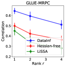
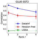
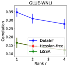
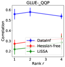
Figure 1: Correlation coefficient comparison of the three influence computation methods. The correlation coefficient captures the similarity to the exact computation of the influence function ((2)), and thus the higher the correlation coefficient, the better. The error bar indicates a 95% confidence interval based on 20 independent runs. DataInf is significantly more correlated with the exact influence values than other methods for all ranks $r\in\{1,2,4\}$, showing better approximation ability. Also, the correlation coefficient of DataInf generally decreases as the rank increases, consistent with our theoretical analysis.

4.2 Mislabeled data detection

Given that mislabeled data points often negatively affect the model performance, it is anticipated that their influence value should be larger than that of clean data points—when they are included, then the loss is likely to increase. In this experiment, we empirically investigate the mislabeled data detection ability of the three influence computation methods as well as the exact influence function ((2)), which we denote by Exact. We consider the same noisy GLUE datasets used in the approximation error analysis. Like the previous experiment, we highlight that annotations for mislabeled data (e.g., one for mislabeled data and zero for clean data) are only used in evaluating the quality of the influence function, not in both fine-tuning and influence computation. As for the evaluation metric, we use the area under the curve (AUC) score between influence values and annotations to capture the order consistency between them. We measure the runtime for computing the influence function for every training data point when one NVIDIA A40 GPU processor is used. The rank $r$ of the LoRA matrix is set to be $4$, but we provide additional experimental results for $r=1$, $r=2$, and $r=8$ in Appendix E, where we find a consistent pattern.

Results

Figure 2 shows that DataInf achieves significantly better detection ability than Hessian-free and LiSSA on all four datasets. Compared to Exact, DataInf presents overall comparable results. Interestingly, we find that DataInf is sometimes better than Exact. We believe many factors including the choice of the damping parameter $\lambda_{l}$ can cause the degradation of Exact, but we leave a rigorous analysis of this as a future research topic. We emphasize that DataInf is also very computationally efficient. In particular, when GLUE-QQP is used, DataInf takes 13 seconds while LiSSA and Exact take 70 and 11279 seconds, respectively, for computing 4500 influence function values. Across the four datasets, ours is $5.5$ and $1149.6$ times faster than LiSSA and Exact, respectively, on average. While Hessian-free is shown to be the fastest method as it does not require to compute the Hessian, its performance is strictly worse than DataInf.

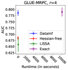
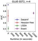
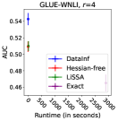
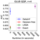
Figure 2: Mislabeled data detection ability comparison of the four influence computation methods when the rank of LoRA matrix $r$ is $4$. The detection ability is evaluated with AUC, and the error bar indicates a 95% confidence interval based on 20 independent runs. DataInf shows better than or comparable detection ability to Exact, and it significantly outperforms Hessian-free and LiSSA on all four datasets. As for the runtime, DataInf is much faster than Exact, demonstrating the practical effectiveness of our method.

4.3 Influential data identification

To further illustrate the usefulness of DataInf, we assess how accurately it can identify influential data points in text generation and text-to-image generation tasks. We use the Llama-2-13B-chat model [22] for the text generation task, and the stable-diffusion-v1.5 model [2] for the text-to-image generation task. Both models are publicly available and widely used in literature.

We construct three demonstrative datasets for the text generation task: (i) Sentence transformations, (ii) Math word problems (without reasoning), and (iii) Math word problems (with reasoning). The detailed description for each task and dataset is given in Table 3. Each dataset contains 10 distinct classes, with 100 total data points in each class. We partition the 100 examples into 90 training data (used for LoRA) points and 10 test data points. For text-to-image generation, we consider two tasks: (i) style generation and (ii) subject generation. For the style generation task, we combine three publicly available image-text pair datasets where each dataset represents different style: cartoons [35], pixel-art [36], and line sketches [37]. For each style, we use 200 training image-text pairs and 50 test image-text pairs for a total of 600 training data points and 150 test data points. For the subject generation task, we use the DreamBooth dataset [38]. There are 31 different subjects and for each subject, 3 data points are used for the training dataset and 1 to 3 data points are used for the validation dataset. The detailed prompts are provided in Appendix D.

If some training data points are highly influential to a test data point’s loss, then their absolute influence function value should be large—it can have a significant positive or significant negative impact on performance. Based on this intuition, we utilize two evaluation metrics. First, for each test data point, we make a pseudo label for every training data point. This pseudo label is one if its label is the same as the test data point’s label, and zero otherwise. We then compute the AUC between the absolute influence function values and the pseudo labels. Ideally, a large AUC is expected because the same class will have a large impact. We report the average AUC across test data points. We denote this by class detection AUC. Second, for each test data point, we compute the percentage of training points with the same class as the test example among the top $s$ influential training points. Here, $s$ is set to be the number of training examples per class. The most influential data points are determined by the absolute influence function values. We report the average percentage across the test data points and denote this by recall. These metrics are intended to assess how effectively each method can identify training data points that belong to the same class as a test example as more influential than one that belongs to a different class.

Results

Evaluation metrics for each task and model are reported in Table 2. DataInf significantly outperforms Hessian-free on all tasks and across all metrics in identifying influential data. Of note, LiSSA demonstrated significant numerical instability across all four tasks and models, which produced invalid influence values in some runs. Even after gradient rescaling, we observed that LiSSA collapses to Hessian-free across all tasks. We hypothesize that this instability can be attributed to the iterative nature of LiSSA and the high-dimensional nature of large-scale models. Qualitative examples with test examples and the corresponding most and least influential training data points are shown in Figure 3.

Table 2: AUC and recall comparison of Hessian-free and DataInf on influential data identification tasks. LiSSA is excluded in this experiment as it often fails to converge due to its instability. The average and standard error of the AUC and recall across test data points are denoted by “average$\pm$standard error”, and the higher, the better for both metrics. DataInf significantly outperforms Hessian-free in both metrics across 5 different tasks.

Task & Model	Method	Class detection (AUC) $\uparrow$	Class detection (Recall) $\uparrow$
Sentence transformations	Hessian-free	$0.967\pm 0.001$	$0.936\pm 0.022$
Llama-2-13B-chat	DataInf	$\mathbf{1.000\pm 0.000}$	$\mathbf{0.998\pm 0.001}$
Math problems (no reasoning)	Hessian-free	$0.868\pm 0.003$	$0.745\pm 0.049$
Llama-2-13B-chat	DataInf	$\mathbf{0.997\pm 0.000}$	$\mathbf{0.996\pm 0.003}$
Math problems (with reasoning)	Hessian-free	$0.935\pm 0.002$	$0.861\pm 0.042$
Llama-2-13B-chat	DataInf	$\mathbf{0.996\pm 0.000}$	$\mathbf{0.993\pm 0.008}$
Text-to-image style generation	Hessian-free	$0.692\pm 0.007$	$0.533\pm 0.008$
stable-diffusion-v1.5	DataInf	$\mathbf{0.820\pm 0.005}$	$\mathbf{0.687\pm 0.006}$
Text-to-image subject generation	Hessian-free	$0.820\pm 0.000$	$0.210\pm 0.003$
stable-diffusion-v1.5	DataInf	$\mathbf{0.865\pm 0.000}$	$\mathbf{0.315\pm 0.003}$

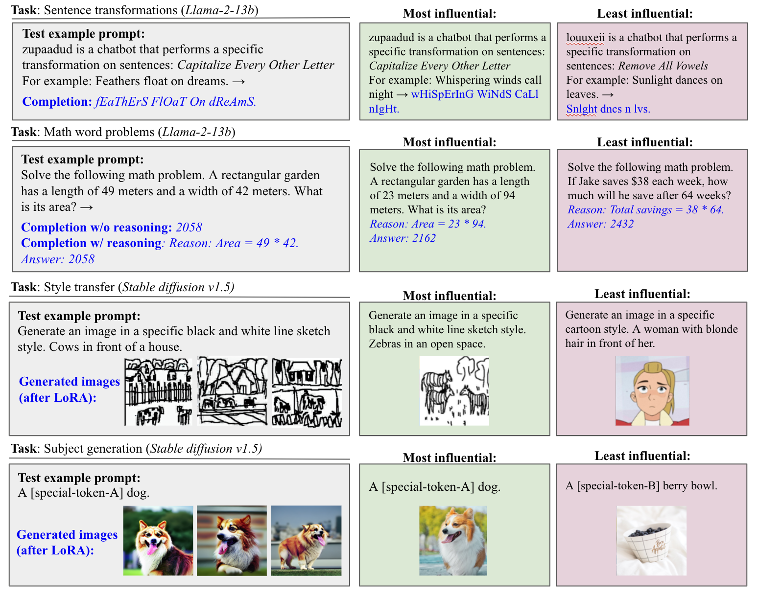
Figure 3: Illustrative examples of most and least influential training data points discovered using DataInf across the text generation and text-to-image generation tasks performed with the Llama-2-13B-chat and stable-diffusion-v1.5 models. The most (resp. least) influential data point has the largest (resp. smallest) absolute influence on the test example among training data points. In the math word problems tasks, separate models are trained with and without an intermediate reasoning step; DataInf effectively finds influential data points.

5 Related works

Evaluating the impact of individual training data points on model accuracy or predictions has been widely studied in data valuation. One of the most widely adopted classes of data valuation methods is based on the marginal contribution, which measures the average change in a model’s performance when a specific data point is removed from a set of data points. Many standard methods belong to this category including leave-one-out and various Shapley-based methods [39, 40, 41, 42]. In addition to these methods, several alternative approaches have been proposed using reinforcement learning [43] or out-of-bag accuracy [44]. Unlike all other data valuation methods, the influence function is based on gradients, conveying the rigorous and intuitive notion of data values. For an extensive review of these methods, we refer the reader to Jiang et al. [45].

When it comes to the empirical performance on downstream machine learning tasks, other data valuation methods often outperform the influence function [46, 45]. However, it is important to note that the majority of previous studies have focused on relatively small models and datasets. This limitation arises from the computational infeasibility of existing data valuation algorithms, as they typically require the training of numerous models to obtain reliable data values [10]. When LLMs or diffusion models are deployed, data valuation methods that require model training are not practically applicable. The development of an efficient computational method is of critical importance, and it is the main contribution of this paper. As a concurrent and independent work, Grosse et al. [14] proposed the Eigenvalue-Kronecker-factored approximate curvature (EK-FAC)-based algorithm that efficiently computes the influence function. While it was applied to LLMs (though not diffusions), the EK-FAC method highly depends on the network architecture, and thus its application to LoRA-tuned models is not straightforward. The implementation of EK-FAC is also not public. We provide a more detailed explanation in Appendix C.

6 Conclusion

We propose DataInf, an efficient influence computation algorithm that is well-suited for parameter-efficient fine-tuning and can be deployed to LLMs and large diffusion models. DataInf is effective in identifying mislabeled data points and retrieving the most and least influential training data points on model generations. DataInf is orders of magnitude faster than state-of-the-art influence computation methods and is memory efficient, and thus it can be practically useful for enabling data-centric analysis of large models such as LLMs.

In the literature, there are not many quantitative evaluation metrics for the utility of influence scores. This also presents limitations for evaluating DataInf. We tried to address it by using proxies such as data points in the same class should have greater influence than data points in a different class, and mislabeled points should increase test loss. Additional downstream of the utility of influence scores for generative AI is an important direction of future work.

Appendix A Proposed algorithm

We provide a pseudo algorithm in Algorithm 1.

Algorithm 1 DataInf: Efficient influence computation

A training dataset $\mathcal{D}=\{(x_{1},y_{1}),\dots,(x_{n},y_{n})\}$, a validation dataset $\mathcal{D}^{\mathrm{(val)}}=\{(x_{1}^{\mathrm{(val)}},y_{1}^{\mathrm{(val)}}),\dots,(x_{m}^{\mathrm{(val)}},y_{m}^{\mathrm{(val)}})\}$, an objective function $\ell\mathrel{\mathop{\mathchar 58\relax}}\mathcal{Y}\times\mathcal{Y}\to\mathbb{R}$, a deep neural network model $f_{\theta}=f_{\theta_{L}}\circ\cdots\circ f_{\theta_{1}}$ where $\theta=\{\theta_{1},\dots,\theta_{L}\}$ and $\theta_{l}\in\mathbb{R}^{d_{l}}$ for $l\in[L]$.

Influence functions $\left\{\mathcal{I}_{\mathrm{DataInf}}(x_{1},y_{1}),\dots,\mathcal{I}_{\mathrm{DataInf}}(x_{n},y_{n})\right\}$.

# Step 1: Compute the first-order gradients

for $l$ in $[L]$ do

     for $i$ in $[n]$ do

         Compute $\nabla_{\theta_{l}}\ell(y_{i},f_{\theta}(x_{i}))$ $\triangleright$ Training data points

     end for

     Compute $\frac{1}{m}\sum_{j=1}^{m}\nabla_{\theta_{l}}\ell(y_{j}^{\mathrm{(val)}},f_{\theta}(x_{j}^{\mathrm{(val)}}))=\mathrel{\mathop{\mathchar 58\relax}}v_{l}$. $\triangleright$ Validation data points

end for

# Step 2: Compute the inverse Hessian-vector product

for $l$ in $[L]$ do

     Compute $\lambda_{l}\mathrel{\mathop{\mathchar 58\relax}}=0.1\times(nd_{l})^{-1}\sum_{i=1}^{n}\nabla_{\theta_{l}}\ell(y_{i},f_{\theta}(x_{i}))^{T}\nabla_{\theta_{l}}\ell(y_{i},f_{\theta}(x_{i}))$

     $v_{l}\leftarrow 0$.

     for $i$ in $[n]$ do

         $c_{li}\leftarrow v_{l}^{T}\nabla_{\theta_{l}}\ell(y_{i},f_{\theta}(x_{i}))/\left(\lambda_{l}+\mathinner{\!\left\lVert\nabla_{\theta_{l}}\ell(y_{i},f_{\theta}(x_{i}))\right\rVert}_{2}^{2}\right)$

         $\triangleright$ A normalizing constant

         $r_{l}\leftarrow r_{l}+(n\lambda_{l})^{-1}\left(v_{l}-c_{li}\nabla_{\theta_{l}}\ell(y_{i},f_{\theta}(x_{i}))\right)$.

     end for

end for

# Step 3: Compute the influence function

for $i$ in $[n]$ do

     $\mathcal{I}_{\mathrm{DataInf}}(x_{k},y_{k})\leftarrow-\sum_{l\in[L]}r_{l}^{T}\nabla_{\theta_{l}}\ell(y_{k},f_{\theta}(x_{k}))$.

end for

Appendix B Proof of Theorem 1

We provide a proof of Theorem 1 below.

Proof.

We set $S_{li}\mathrel{\mathop{\mathchar 58\relax}}=\nabla_{\theta_{l}}\ell_{i}\nabla_{\theta_{l}}\ell_{i}^{T}+\lambda_{l}I_{d_{l}}$ and $\bar{S}_{l}\mathrel{\mathop{\mathchar 58\relax}}=n^{-1}\sum_{i=1}^{n}S_{li}$. Then, a Taylor expansion gives

$$\frac{1}{n}\sum_{i=1}^{n}S_{li}^{-1}-\left(\frac{1}{n}\sum_{i=1}^{n}S_{li}\right)^{-1} =\frac{1}{n}\sum_{i=1}^{n}\left(S_{li}-\bar{S}_{l}\right)^{T}\left(\int_{0}^{1}(tS_{li}+(1-t)\bar{S}_{l})^{-3}dt\right)\left(S_{li}-\bar{S}_{l}\right)$$

$$\preceq\frac{1}{\lambda_{l}^{3}}\frac{1}{n}\sum_{i=1}^{n}\left(S_{li}-\bar{S}_{l}\right)\left(S_{li}-\bar{S}_{l}\right)^{T}.$$

The inequality is due to the maximum eigenvalue of $(tS_{li}+(1-t)\bar{S}_{l})^{-3}$ is upper bounded by $\lambda_{l}^{-3}$ for $0<t<1$. Then, the spectral norm of this matrix is upper bounded as follows:

$$\mathinner{\!\left\lVert\frac{1}{\lambda_{l}^{3}}\frac{1}{n}\sum_{i=1}^{n}\left(S_{li}-\bar{S}_{l}\right)\left(S_{li}-\bar{S}_{l}\right)^{T}\right\rVert}_{2} \leq\frac{1}{\lambda_{l}^{3}}\frac{1}{n}\sum_{i=1}^{n}\mathinner{\!\left\lVert S_{li}-\bar{S}_{l}\right\rVert}_{2}^{2}$$

$$\leq\frac{1}{\lambda_{l}^{3}}\frac{1}{n}\sum_{i=1}^{n}\left(\mathinner{\!\left\lVert S_{li}\right\rVert}_{2}+\mathinner{\!\left\lVert\bar{S}_{l}\right\rVert}_{2}\right)^{2}.$$

The first inequality is due to the triangle inequality and the second inequality is from $\lambda_{\mathrm{max}}(A-B)\leq\lambda_{\mathrm{max}}(A)+\lambda_{\mathrm{max}}(B)$ for real symmetric matrices $A$ and $B$. Here, $\lambda_{\mathrm{max}}(A)$ denotes the largest eigenvalue of a matrix $A$.

For all $l\in[L]$ and $i\in[n]$, since $S_{li}$ is a semi-positive definite matrix, we have $\mathinner{\!\left\lVert S_{li}\right\rVert}_{2}=\lambda_{\mathrm{max}}(S_{li})\leq\mathrm{tr}(S_{li})$ and $\mathinner{\!\left\lVert\bar{S}_{l}\right\rVert}_{2}=\lambda_{\mathrm{max}}(\bar{S}_{l})\leq\mathrm{tr}(\bar{S}_{l})$. Hence,

$$\frac{1}{\lambda_{l}^{3}}\frac{1}{n}\sum_{i=1}^{n}\left(\mathinner{\!\left\lVert S_{li}\right\rVert}_{2}+\mathinner{\!\left\lVert\bar{S}_{l}\right\rVert}_{2}\right)^{2}\leq\frac{1}{\lambda_{l}^{3}}\frac{1}{n}\sum_{i=1}^{n}\left(\mathrm{tr}\left(S_{li}\right)+\mathrm{tr}\left(\bar{S}_{l}\right)\right)^{2}.$$

Since $\mathinner{\!\left\lVert\nabla_{\theta_{l}}\ell_{i}\right\rVert}_{\infty}$ is upper bounded by a constant, there exists a constant $M>0$ such that $\mathrm{tr}\left(S_{li}\right)+\mathrm{tr}\left(\bar{S}_{l}\right)\leq Md_{l}$. This implies that:

$$\frac{1}{\lambda_{l}^{3}}\frac{1}{n}\sum_{i=1}^{n}\left(\mathinner{\!\left\lVert S_{li}\right\rVert}_{2}+\mathinner{\!\left\lVert\bar{S}_{l}\right\rVert}_{2}\right)^{2}\leq\frac{M^{2}d_{l}^{2}}{\lambda_{l}^{3}}=O(d_{l}^{2}).$$

∎

Appendix C Existing methods

In this section, we provide three existing influence computation methods: EK-FAC and retraining-based methods.

EK-FAC

To this end, we suppose $f_{\theta}$ is a multilayer perceptron model. For $l\in[L]$, we denote the $l$-th layer output by $h_{l}\mathrel{\mathop{\mathchar 58\relax}}=f_{\theta_{l}}\circ\cdots\circ f_{\theta_{1}}$ and the associated pre-activated output by $g_{l}$. Then, for all $k\in[n]$, we have $\nabla_{\theta_{l}}\ell_{k}=h_{l-1}(x_{k})\otimes\nabla_{g_{l}}\ell_{k}$ where $\otimes$ denotes the Kronecker product. Moreover, the Hessian for $\theta_{l}$ is given as follows:

$$G_{l}(\theta^{*}) =\frac{1}{n}\sum_{i=1}^{n}\left(h_{l-1}(x_{i})\otimes\nabla_{g_{l}}\ell_{i}\right)\left(h_{l-1}(x_{i})\otimes\nabla_{g_{l}}\ell_{i}\right)^{T}$$

$$=\frac{1}{n}\sum_{i=1}^{n}\left(h_{l-1}(x_{i})h_{l-1}(x_{i})^{T}\right)\otimes\left(\nabla_{g_{l}}\ell_{i}\nabla_{g_{l}}\ell_{i}^{T}\right)$$

The second equality is due to the mixed-product property of the Kronecker product. George et al. [19] proposed to approximate $G_{l}(\theta^{*})$ with the following equation:

$$G_{l}(\theta^{*})\approx\frac{1}{n}\sum_{i=1}^{n}h_{l-1}(x_{i})h_{l-1}(x_{i})^{T}\otimes\frac{1}{n}\sum_{i=1}^{n}\nabla_{g_{l}}\ell_{i}\nabla_{g_{l}}\ell_{i}^{T}=\mathrel{\mathop{\mathchar 58\relax}}A_{l-1}\otimes B_{l}$$

This approximation is accurate when one of the following approximations holds:

$$\nabla_{g_{l}}\ell_{i}\nabla_{g_{l}}\ell_{i}^{T}\approx\frac{1}{n}\sum_{j=1}^{n}\nabla_{g_{l}}\ell_{j}\nabla_{g_{l}}\ell_{j}^{T}\quad\forall i\in[n],$$ (6)

or

$$h_{l-1}(x_{i})h_{l-1}(x_{i})^{T}\approx\frac{1}{n}\sum_{j=1}^{n}h_{l-1}(x_{j})h_{l-1}(x_{j})^{T}\quad\forall i\in[n].$$ (7)

The assumptions in (6) and (7) essentially assume that $h_{l-1}$ and $\nabla_{g_{l}}\ell$ are constant across different training data points. While there is no clear intuition, the approximation leads to a computationally efficient form. Specifically, we let $A_{l-1}=Q_{A_{l-1}}\Lambda_{A_{l-1}}Q_{A_{l-1}}^{T}$ where $Q_{A_{l-1}}$ is an orthonormal matrix and $\Lambda_{A_{l-1}}$ is a diagonal matrix obtained by eigenvalue decomposition. Similarly, we factorize $B_{l}=Q_{B_{l}}\Lambda_{B_{l}}Q_{B_{l}}^{T}$. Then, we have:

$$(G_{l}(\theta^{*})+\lambda_{l}I_{d_{l}})^{-1}=(Q_{A_{l-1}}\otimes Q_{B_{l}})(\Lambda_{A_{l-1}}\otimes\Lambda_{B_{l}}+\lambda_{l}I_{d_{l}})^{-1}(Q_{A_{l-1}}\otimes Q_{B_{l}})^{T}$$

That is, $(G_{l}(\theta^{*})+\lambda_{l}I_{d_{l}})^{-1}$ can be obtained by applying eigenvalue decomposition of $A_{l-1}$ and $B_{l}$. Compared to naive matrix inversion $(G_{l}(\theta^{*})+\lambda_{l}I_{d_{l}})^{-1}$, this approximation method has computational efficiency as the size of $A_{l-1}$ and $B_{l}$ is much smaller than $d_{l}$. This method is called Kronecker Factorization, also known as KFAC. George et al. [19] showed that that using $\Lambda_{A_{l-1}}\otimes\Lambda_{B_{l}}$ can be suboptimal in approximating with a diagonal matrix $\Lambda$ where the $i$-th diagonal element is set to be $\Lambda_{ii}=n^{-1}\sum_{j=1}^{n}((Q_{A_{l-1}}\otimes Q_{B_{l}})\nabla_{\theta_{l}}\ell_{j})_{i}^{2}$. A naive computation of the left-hand side requires $O(d_{l}^{3})$ operations, but both KFAC and EK-FAC can be done in $O(d_{l}^{3/2})$ operations when the size of both $A_{l-1}$ and $B_{l}$ is $\sqrt{d_{l}}$. Hence, the total computational complexity is $O(\sum_{l=1}^{L}(nd_{l}+d_{l}^{3/2}))$ with $O(\max_{l\in[L]}d_{l}^{2})$ memory complexity.

EK-FAC has a computational advantage over a naive version of LiSSA, but it might not be applicable to general deep neural network models as it highly depends on the model architecture—the gradient should be expressed as $\nabla_{\theta_{l}}\ell_{k}=h_{l-1}(x_{k})\otimes\nabla_{g_{l}}\ell_{k}$, which it might not be true for LoRA fine-tuned models or transformer-based models. This method has been used in an independent and concurrent work [14].

Retraining-based method

For $M\in[n]$, we denote a set of subsets with the same cardinality by $\mathcal{S}^{(M)}\mathrel{\mathop{\mathchar 58\relax}}=\{S\mathrel{\mathop{\mathchar 58\relax}}S\subseteq\mathcal{D},|S|=M\}$. For $i\in[n]$, we set $\mathcal{S}_{i,\mathrm{in}}^{(M)}\mathrel{\mathop{\mathchar 58\relax}}=\{S\in\mathcal{S}^{(M)}\mathrel{\mathop{\mathchar 58\relax}}(x_{i},y_{i})\in S\}$ and $\mathcal{S}_{i,\mathrm{out}}^{(M)}\mathrel{\mathop{\mathchar 58\relax}}=\{S\in\mathcal{S}^{(M)}\mathrel{\mathop{\mathchar 58\relax}}(x_{i},y_{i})\notin S\}$. Note that $\mathcal{S}_{i,\mathrm{in}}^{(M)}\cup\mathcal{S}_{i,\mathrm{out}}^{(M)}=\mathcal{S}$ and $\mathcal{S}_{i,\mathrm{in}}^{(M)}\cap\mathcal{S}_{i,\mathrm{out}}^{(M)}=\{\}$ for all $i\in[n]$. Feldman and Zhang [10] proposed to compute the influence of a data point $(x_{i},y_{i})\in\mathcal{D}$ on a loss value $\ell(y^{*},f_{\theta^{*}}(x^{*}))$ as a difference of model outputs.

$$\frac{1}{|\mathcal{S}_{i,\mathrm{in}}^{(M)}|}\sum_{S\in\mathcal{S}_{i,\mathrm{in}}^{(M)}}\ell(y^{*},f_{\theta_{S}}(x^{*}))-\frac{1}{|\mathcal{S}_{i,\mathrm{out}}^{(M)}|}\sum_{S\in\mathcal{S}_{i,\mathrm{out}}^{(M)}}\ell(y^{*},f_{\theta_{S}}(x^{*})),$$

where

$$\theta_{S}\mathrel{\mathop{\mathchar 58\relax}}=\mathrm{argmin}_{\theta\in\Theta}\frac{1}{|S|}\sum_{i\in S}\ell(y_{i},f_{\theta}(x_{i})).$$

This retraining-based method is flexible in that any deep neural network model can be used for $f_{\theta}$, however, it is extremely challenging to compute because it necessitates the training of numerous models.

Appendix D Implementation details

In this section, we provide implementation details on datasets, models, and loss functions we used in Section 4. We also provide the Python-based implementation codes at https://github.com/ykwon0407/DataInf.

D.1 Approximation error analysis and Mislabeled data detection

Datasets

We consider the four binary classification GLUE benchmarking datasets [34]. Namely, the four datasets are GLUE-MARPC [48, paraphrase detection], GLUE-SST2 [49, sentiment analysis], GLUE-WNLI [50, inference], and GLUE-QQP (question-answering). We used the training and validation splits of the dataset available at HuggingFace Datasets library [51]. Only the training dataset is used to fine-tune the model, and we compute the influence of individual training data points on the validation loss. For GLUE-SST2 and GLUE-QQP, we randomly sample 4500 (resp. 500) samples from the original training (resp. validation) dataset.

Model

We use LoRA to fine-tune the RoBERTa-large model, a 355M parameter LLM trained on the large-scale publicly available natural language datasets [21]. We apply LoRA to every value matrix of the attention layers of the RoBERTa-large model. We downloaded the pre-trained model from the HuggingFace Transformers library [52]. Across all fine-tuning runs, we use a learning rate of $3\times 10^{-4}$ with a batch size of 32 across 10 training epochs. As for the LoRA hyperparameters, the dropout rate is set to be $0.05$. We choose the rank of the LoRA matrix $r$ from $\{1,2,4,8\}$ and $\alpha$ is always set to be $r$. The training was performed on a single machine with one NVIDIA A40 GPU using the HuggingFace Peft library [53].

Loss

All GLUE benchmarking datasets we used are binary classification datasets, so we used a negative log-likelihood function as a loss function. For a sequence of input tokens $x=(x_{1},\dots,x_{T})$ and its label $y$, we consider $\ell(y,f_{\theta}(x))=-\log p(y\mid f_{\theta}(x))$ where $f_{\theta}$ is a composition model consists of the RoBERTa-large model to convert text data into numerical embeddings, and a logistic model to perform classification on the embedding space. We set $T=128$.

D.2 Influential data identification

D.2.1 Text generation

Datasets

Full dataset prompts are described in Tables 5 and 6.

Model

We use LoRA to fine-tune Llama-2-13B-chat, an LLM that has 13 billion parameters, is pre-trained on 2 trillion tokens, and is optimized for dialogue use cases [22]. We apply LoRA to every query and value matrix of the attention layer in the Llama-2-13B-chat model. Across all fine-tuning runs, we use a learning rate of $3\times 10^{-4}$, LoRA hyperparameters $r=8$ and $\alpha=32$, in 8-bit quantization, with a batch size of 64 across 25 training epochs. The training was performed on a single machine with 4 NVIDIA V100 GPUs using the HuggingFace Peft library [53].

Loss

We used a negative log-likelihood of a generated response as a loss function. For a sequence of input tokens $x=(x_{1},\dots,x_{T_{1}})$ and the corresponding sequence of target tokens $y=(y_{1},\dots,y_{T_{2}})$, suppose the Llama-2-13B generates a sequence of output tokens $f_{\theta}(x)=(f_{\theta}(x)_{1},\dots,f_{\theta}(x)_{T_{2}})$. $f_{\theta}(x)$ has the same size of $T_{2}$ and is generated in an auto-regressive manner. We set $T_{1}=T_{2}=512$. Then, the loss function is $\ell(y,f_{\theta}(x))=-\sum_{t=1}^{T_{2}}\log p(y_{t}\mid f_{\theta}(x)_{1},\dots,f_{\theta}(x)_{t-1})$.

Experiments

The test accuracy for the base (non-fine-tuned) and fine-tuned models is shown in Table 4. We observe substantial improvements across the three tasks, with additional improvements from introducing an intermediate reasoning step to the math word problems.

D.2.2 Text-to-image generation - style generation

Datasets

Figure 4 illustrates examples of images used in the text-to-image generation task. When we fine-tuned a model, a style description is added to a text sequence to instruct a style. For instance, “Generate an image in a specific {custom} style. {text-data}”, where {custom} is substituted with either “cartoon”, “pixelart”, or “black and white line sketch”, and {text-data} is substituted with a text sequence in the training dataset. We provide a detailed description in Table 7.

Model

We also use LoRA to fine-tune stable-diffusion-v1.5 [2]. We apply LoRA to every attention layer in the stable-diffusion-v1.5 model. Across all fine-tuning runs, we use a learning rate of $10^{-4}$, LoRA hyperparameters $r=1$ and $\alpha=1$. We fine-tune a model with a batch size of 4 across 10000 training steps. The training was performed on a single machine with 4 NVIDIA V100 GPUs using the HuggingFace Peft library [53].

Loss

Similar to other experiments, we used a negative log-likelihood of a generated image as a loss function. For a sequence of input tokens $x=(x_{1},\dots,x_{T})$ and the corresponding target image $y$, we can compute a negative log-likelihood $\ell(y,f_{\theta}(x))=-\log p(y\mid f_{\theta}(x))$. We set $T=77$.

Experiment

We compare generated images before and after the LoRA fine-tuning. For quantitative comparison, the baseline and fine-tuned models are evaluated by comparing the Fréchet inception distance (FID) between images in the test set with images generated using the paired texts from the test set. FID for the before and after fine-tuning models is shown in Table 4.

D.2.3 Text-to-image generation - subject generation

We used the same setting with the text-to-image generation style generation task, but the rank of LoRA matrices is set to $4$. We here explain the datasets.

Datasets

Figure 4 illustrates examples of images used in the text-to-image generation task. Our models use Google’s Dreambooth dataset [38], which contains 31 unique subjects in categories like backpack, dog, bowl, and sneaker. Each subject has four to six total examples, and we take three from each subject as the training set, with the remaining as the validation. We add a unique random string to each subject to prompt the model to produce each subject. For example, to differentiate two different dogs, we use prompts "a 5a2PZ dog" and "a POVRB dog" in the training and test set.

Table 3: Description of each task and dataset used in Section 4.3. For the text generation task, we describe the full dataset prompts in Table 5.

Task	Description
Sentence transformations	The model is asked to perform a specific transformation on a sentence. Ten different types of sentence transformations are used. To aid the model in learning distinct transformations, “chatbot” name identifiers that are uniquely associated with each transformation are added to the prompts.
Math problems (without reasoning)	The model is asked to provide a direct answer to a simple arithmetic word problem. Ten different types of math word problems are constructed, and random positive integers are used to construct unique data points.
Math problems (with reasoning)	Using the same questions with as above (Math problems without reasoning), the prompt includes an intermediate reasoning step before arriving at the final answer.
Text-to-image style generation	The model is asked to generate an image in a given style. Three different styles of images are used in our dataset. We illustrate examples of styles in Figure 4.
Text-to-image subject generation	The model is asked to generate a specific subject (e.g. a dog or a candle). We illustrate examples of styles in Figure 4.

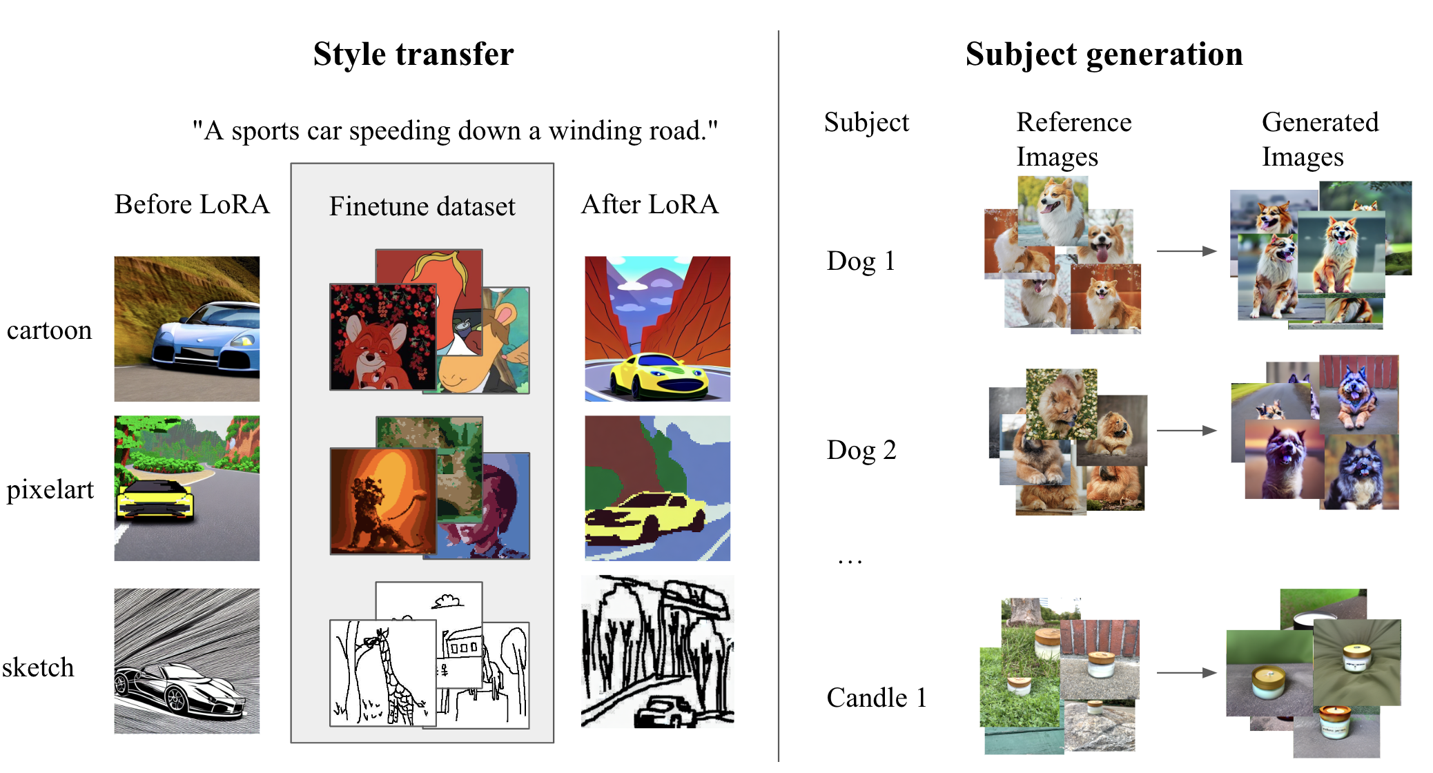
Figure 4: Examples of images used in the text-to-image generation task, along with before and after images from the LoRA fine-tuning of the stable-diffusion-v1.5 model.

Table 4: Performance improvements from model fine-tuning. For the text generation tasks, we evaluate the classification accuracy. For the text-to-image generation task, we evaluate FID.

Task	Method	Accuracy $\uparrow$	FID $\downarrow$
Sentence transformations	Base model	0.01	-
	Fine-tuned model	0.35	-
Math problems (no reasoning)	Base model	0.07	-
	Fine-tuned model	0.20	-
Math problems (with reasoning)	Base model	0.08	-
	Fine-tuned model	0.31	-
Text-to-image style generation	Base model	-	243.5
	Fine-tuned model	-	189.6
Text-to-image subject generation	Base model	-	269.7
	Fine-tuned model	-	247.5

Table 5: Description of the sentence transformations task templates. We consider 10 different types of sentence transformations. For each sentence transformation, unique identifying “chatbot” names were additionally prepended to the task prompt to assist the model in training.

Sentence transformations	Example transformation of “Sunrises herald hopeful tomorrows”:
Reverse Order of Words	tomorrows. hopeful herald Sunrises
Capitalize Every Other Letter	sUnRiSeS hErAlD hOpEfUl tOmOrRoWs.
Insert Number 1 Between Every Word	Sunrises 1herald 1hopeful 1tomorrows.
Replace Vowels with *	S*nr*s*s h*r*ld h*p*f*l t*m*rr*ws.
Double Every Consonant	SSunrriisseess hheralld hhopeffull ttomorrows.
Capitalize Every Word	Sunrises Herald Hopeful Tomorrows.
Remove All Vowels	Snrss hrld hpfl tmrrws.
Add ’ly’ To End of Each Word	Sunrisesly heraldly hopefully tomorrows.ly
Remove All Consonants	uie ea oeu ooo.
Repeat Each Word Twice	Sunrises Sunrises herald herald hopeful hopeful tomorrows. tomorrows.

Table 6: Description of the math problem task templates. We consider 10 different types of math word problems.

Math Word Problems	Template prompt question
Remaining pizza slices	Lisa ate A slices of pizza and her brother ate B slices from a pizza that originally had C slices. How many slices of the pizza are left?
	Reason: Combined slices eaten = A + B. Left = C - (A + B).
Chaperones needed for trip	For every A students going on a field trip, there are B adults needed as chaperones. If C students are attending, how many adults are needed?
	Reason: Adults needed = (B * C) // A.
Total number after purchase	In an aquarium, there are A sharks and B dolphins. If they bought C more sharks, how many sharks would be there in total?
	Reason: Total sharks = A + C.
Total game points	Michael scored A points in the first game, B points in the second, C in the third, and D in the fourth game. What is his total points?
	Reason: Total points = A + B + C + D.
Total reading hours	Emily reads for A hours each day. How many hours does she read in total in B days?
	Reason: Total hours read = A * B.
Shirt cost after discount	A shirt costs A. There’s a B-dollar off sale. How much does the shirt cost after the discount?
	Reason: Cost after discount = A - B.
Area of a garden	A rectangular garden has a length of A meters and a width of B meters. What is its area?
	Reason: Area = A * B.
Total savings	If Jake saves A each week, how much will he save after B weeks?
	Reason: Total savings = A * B.
Number of cupcake boxes	A bakery sells cupcakes in boxes of A. If they have B cupcakes, how many boxes can they fill?
	Reason: Boxes filled = B // A.
Interest earned	John invests A at an annual interest rate of B%. How much interest will he earn after C years?
	Reason: Interest = (A * B * C) // 100.

Table 7: Description of the text-to-image generation task templates. Each style has 200 training image-text pairs and 150 validation image-text pairs.

Image style	Text prompt
Cartoon	Generate an image in a specific cartoon style. {A text sequence of the original dataset which describes an image}.
Pixel Art	Generate an image in a specific pixelart style. {A text sequence of the original dataset which describes an image}.
Sketch	Generate an image in a specific black and white line sketch style. {A text sequence of the original dataset which describes an image}.

Appendix E Additional experimental results

Mislabeled data detection task.

We provide additional mislabeled data detection task results when the rank $r$ is selected from $\{1,2,8\}$. We exclude Exact when $r=8$ because it exceeds the 12-hour computation limit for all datasets. In this case, DataInf takes less than 25 seconds. Similar to the case $r=4$, DataInf shows competitive mislabeled detection performance over other methods while achieving a short runtime.

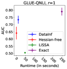
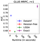
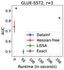
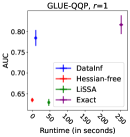
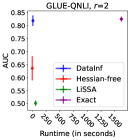
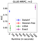
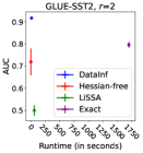
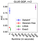
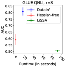
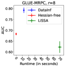
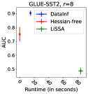
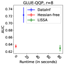
Figure 5: Mislabeled data detection task ability comparison of the four influence computation methods when the rank of LoRA matrix $r$ is (top) $1$, (middle) $2$, and (bottom) $8$. The error bar indicates a 95% confidence interval based on 20 independent runs. Similar to Figure 2, DataInf shows superior detection ability while achieving competitive computational efficiency.

References

- Brown et al. [2020] Tom Brown, Benjamin Mann, Nick Ryder, Melanie Subbiah, Jared D Kaplan, Prafulla Dhariwal, Arvind Neelakantan, Pranav Shyam, Girish Sastry, Amanda Askell, et al. Language models are few-shot learners. Advances in neural information processing systems, 33:1877–1901, 2020.
- Rombach et al. [2022] Robin Rombach, Andreas Blattmann, Dominik Lorenz, Patrick Esser, and Björn Ommer. High-resolution image synthesis with latent diffusion models. In Proceedings of the IEEE/CVF conference on computer vision and pattern recognition, pages 10684–10695, 2022.
- Jiao et al. [2023] Wenxiang Jiao, Wenxuan Wang, Jen-tse Huang, Xing Wang, and Zhaopeng Tu. Is chatgpt a good translator? a preliminary study. arXiv preprint arXiv:2301.08745, 2023.
- Abid et al. [2021] Abubakar Abid, Maheen Farooqi, and James Zou. Persistent anti-muslim bias in large language models. In Proceedings of the 2021 AAAI/ACM Conference on AI, Ethics, and Society, pages 298–306, 2021.
- Ouyang et al. [2022] Long Ouyang, Jeffrey Wu, Xu Jiang, Diogo Almeida, Carroll Wainwright, Pamela Mishkin, Chong Zhang, Sandhini Agarwal, Katarina Slama, Alex Ray, et al. Training language models to follow instructions with human feedback. Advances in Neural Information Processing Systems, 35:27730–27744, 2022.
- Ferrara [2023] Emilio Ferrara. Should chatgpt be biased? challenges and risks of bias in large language models. arXiv preprint arXiv:2304.03738, 2023.
- Hampel [1974] Frank R Hampel. The influence curve and its role in robust estimation. Journal of the American Statistical Association, 69(346):383–393, 1974.
- Cook and Weisberg [1980] R Dennis Cook and Sanford Weisberg. Characterizations of an empirical influence function for detecting influential cases in regression. Technometrics, 22(4):495–508, 1980.
- Koh and Liang [2017] Pang Wei Koh and Percy Liang. Understanding black-box predictions via influence functions. In International conference on machine learning, pages 1885–1894. PMLR, 2017.
- Feldman and Zhang [2020] Vitaly Feldman and Chiyuan Zhang. What neural networks memorize and why: Discovering the long tail via influence estimation. Advances in Neural Information Processing Systems, 33:2881–2891, 2020.
- Guo et al. [2021] Han Guo, Nazneen Rajani, Peter Hase, Mohit Bansal, and Caiming Xiong. Fastif: Scalable influence functions for efficient model interpretation and debugging. In Proceedings of the 2021 Conference on Empirical Methods in Natural Language Processing, pages 10333–10350, 2021.
- Han et al. [2020] Xiaochuang Han, Byron C Wallace, and Yulia Tsvetkov. Explaining black box predictions and unveiling data artifacts through influence functions. In Proceedings of the 58th Annual Meeting of the Association for Computational Linguistics. Association for Computational Linguistics, 2020.
- Aamir et al. [2023] Aisha Aamir, Minija Tamosiunaite, and Florentin Wörgötter. Interpreting the decisions of cnns via influence functions. Frontiers in Computational Neuroscience, 17, 2023.
- Grosse et al. [2023] Roger Grosse, Juhan Bae, Cem Anil, Nelson Elhage, Alex Tamkin, Amirhossein Tajdini, Benoit Steiner, Dustin Li, Esin Durmus, Ethan Perez, et al. Studying large language model generalization with influence functions. arXiv preprint arXiv:2308.03296, 2023.
- Wang et al. [2019] Hao Wang, Berk Ustun, and Flavio Calmon. Repairing without retraining: Avoiding disparate impact with counterfactual distributions. In International Conference on Machine Learning, pages 6618–6627. PMLR, 2019.
- Kong et al. [2022] Shuming Kong, Yanyan Shen, and Linpeng Huang. Resolving training biases via influence-based data relabeling. In International Conference on Learning Representations, 2022. URL https://openreview.net/forum?id=EskfH0bwNVn.
- Martens [2010] James Martens. Deep learning via hessian-free optimization. In Proceedings of the 27th International Conference on International Conference on Machine Learning, pages 735–742, 2010.
- Agarwal et al. [2017] Naman Agarwal, Brian Bullins, and Elad Hazan. Second-order stochastic optimization for machine learning in linear time. The Journal of Machine Learning Research, 18(1):4148–4187, 2017.
- George et al. [2018] Thomas George, César Laurent, Xavier Bouthillier, Nicolas Ballas, and Pascal Vincent. Fast approximate natural gradient descent in a kronecker factored eigenbasis. Advances in Neural Information Processing Systems, 31, 2018.
- Devlin et al. [2018] Jacob Devlin, Ming-Wei Chang, Kenton Lee, and Kristina Toutanova. Bert: Pre-training of deep bidirectional transformers for language understanding. arXiv preprint arXiv:1810.04805, 2018.
- Liu et al. [2019] Yinhan Liu, Myle Ott, Naman Goyal, Jingfei Du, Mandar Joshi, Danqi Chen, Omer Levy, Mike Lewis, Luke Zettlemoyer, and Veselin Stoyanov. Roberta: A robustly optimized bert pretraining approach. arXiv preprint arXiv:1907.11692, 2019.
- Touvron et al. [2023] Hugo Touvron, Louis Martin, Kevin Stone, Peter Albert, Amjad Almahairi, Yasmine Babaei, Nikolay Bashlykov, Soumya Batra, Prajjwal Bhargava, Shruti Bhosale, et al. Llama 2: Open foundation and fine-tuned chat models. arXiv preprint arXiv:2307.09288, 2023.
- Sohl-Dickstein et al. [2015] Jascha Sohl-Dickstein, Eric Weiss, Niru Maheswaranathan, and Surya Ganguli. Deep unsupervised learning using nonequilibrium thermodynamics. In International conference on machine learning, pages 2256–2265. PMLR, 2015.
- Ho et al. [2020] Jonathan Ho, Ajay Jain, and Pieter Abbeel. Denoising diffusion probabilistic models. Advances in neural information processing systems, 33:6840–6851, 2020.
- Martin and Yohai [1986] R Douglas Martin and Victor J Yohai. Influence functionals for time series. The annals of Statistics, pages 781–818, 1986.
- Van der Vaart [2000] Aad W Van der Vaart. Asymptotic statistics, volume 3. Cambridge university press, 2000.
- Bartlett [1953] MS Bartlett. Approximate confidence intervals. Biometrika, 40(1/2):12–19, 1953.
- Basu et al. [2020] Samyadeep Basu, Phil Pope, and Soheil Feizi. Influence functions in deep learning are fragile. In International Conference on Learning Representations, 2020.
- Bae et al. [2022] Juhan Bae, Nathan Ng, Alston Lo, Marzyeh Ghassemi, and Roger B Grosse. If influence functions are the answer, then what is the question? Advances in Neural Information Processing Systems, 35:17953–17967, 2022.
- Schioppa et al. [2022] Andrea Schioppa, Polina Zablotskaia, David Vilar, and Artem Sokolov. Scaling up influence functions. In Proceedings of the AAAI Conference on Artificial Intelligence, volume 36, pages 8179–8186, 2022.
- Hu et al. [2021] Edward J Hu, Phillip Wallis, Zeyuan Allen-Zhu, Yuanzhi Li, Shean Wang, Lu Wang, Weizhu Chen, et al. Lora: Low-rank adaptation of large language models. In International Conference on Learning Representations, 2021.
- Charpiat et al. [2019] Guillaume Charpiat, Nicolas Girard, Loris Felardos, and Yuliya Tarabalka. Input similarity from the neural network perspective. Advances in Neural Information Processing Systems, 32, 2019.
- Pruthi et al. [2020] Garima Pruthi, Frederick Liu, Satyen Kale, and Mukund Sundararajan. Estimating training data influence by tracing gradient descent. Advances in Neural Information Processing Systems, 33:19920–19930, 2020.
- Wang et al. [2018] Alex Wang, Amanpreet Singh, Julian Michael, Felix Hill, Omer Levy, and Samuel R Bowman. Glue: A multi-task benchmark and analysis platform for natural language understanding. arXiv preprint arXiv:1804.07461, 2018.
- Norod78 [2023] Norod78. Norod78/cartoon-blip-captions · Datasets at Hugging Face — huggingface.co. https://huggingface.co/datasets/Norod78/cartoon-blip-captions, 2023. [Accessed 24-09-2023].
- Jainr3 [2023] Jainr3. jainr3/diffusiondb-pixelart · Datasets at Hugging Face — huggingface.co. https://huggingface.co/datasets/jainr3/diffusiondb-pixelart, 2023. [Accessed 24-09-2023].
- Zoheb [2023] Zoheb. zoheb/sketch-scene · Datasets at Hugging Face — huggingface.co. https://huggingface.co/datasets/zoheb/sketch-scene, 2023. [Accessed 24-09-2023].
- Ruiz et al. [2023] Nataniel Ruiz, Yuanzhen Li, Varun Jampani, Yael Pritch, Michael Rubinstein, and Kfir Aberman. Dreambooth: Fine tuning text-to-image diffusion models for subject-driven generation. In Proceedings of the IEEE/CVF Conference on Computer Vision and Pattern Recognition, pages 22500–22510, 2023.
- Ghorbani and Zou [2019] Amirata Ghorbani and James Zou. Data shapley: Equitable valuation of data for machine learning. In International Conference on Machine Learning, pages 2242–2251, 2019.
- Jia et al. [2019] Ruoxi Jia, David Dao, Boxin Wang, Frances Ann Hubis, Nezihe Merve Gurel, Bo Li, Ce Zhang, Costas Spanos, and Dawn Song. Efficient task-specific data valuation for nearest neighbor algorithms. Proceedings of the VLDB Endowment, 12(11):1610–1623, 2019.
- Kwon and Zou [2022] Yongchan Kwon and James Zou. Beta shapley: a unified and noise-reduced data valuation framework for machine learning. In International Conference on Artificial Intelligence and Statistics, pages 8780–8802. PMLR, 2022.
- Wang and Jia [2023] Jiachen T. Wang and Ruoxi Jia. Data banzhaf: A robust data valuation framework for machine learning. Proceedings of The 26th International Conference on Artificial Intelligence and Statistics, 206:6388–6421, 2023.
- Yoon et al. [2020] Jinsung Yoon, Sercan Arik, and Tomas Pfister. Data valuation using reinforcement learning. In International Conference on Machine Learning, pages 10842–10851. PMLR, 2020.
- Kwon and Zou [2023] Yongchan Kwon and James Zou. Data-oob: Out-of-bag estimate as a simple and efficient data value. 2023.
- Jiang et al. [2023] Kevin Fu Jiang, Weixin Liang, James Zou, and Yongchan Kwon. Opendataval: a unified benchmark for data valuation, 2023.
- Park et al. [2023] Sung Min Park, Kristian Georgiev, Andrew Ilyas, Guillaume Leclerc, and Aleksander Madry. Trak: Attributing model behavior at scale. arXiv preprint arXiv:2303.14186, 2023.
- Bach [2022] Francis Bach. Information theory with kernel methods. IEEE Transactions on Information Theory, 69(2):752–775, 2022.
- Dolan and Brockett [2005] Bill Dolan and Chris Brockett. Automatically constructing a corpus of sentential paraphrases. In Third International Workshop on Paraphrasing (IWP2005), 2005.
- Socher et al. [2013] Richard Socher, Alex Perelygin, Jean Wu, Jason Chuang, Christopher D Manning, Andrew Y Ng, and Christopher Potts. Recursive deep models for semantic compositionality over a sentiment treebank. In Proceedings of the 2013 conference on empirical methods in natural language processing, pages 1631–1642, 2013.
- Levesque et al. [2012] Hector Levesque, Ernest Davis, and Leora Morgenstern. The winograd schema challenge. In Thirteenth international conference on the principles of knowledge representation and reasoning, 2012.
- Lhoest et al. [2021] Quentin Lhoest, Albert Villanova del Moral, Yacine Jernite, Abhishek Thakur, Patrick von Platen, Suraj Patil, Julien Chaumond, Mariama Drame, Julien Plu, Lewis Tunstall, Joe Davison, Mario Šaško, Gunjan Chhablani, Bhavitvya Malik, Simon Brandeis, Teven Le Scao, Victor Sanh, Canwen Xu, Nicolas Patry, Angelina McMillan-Major, Philipp Schmid, Sylvain Gugger, Clément Delangue, Théo Matussière, Lysandre Debut, Stas Bekman, Pierric Cistac, Thibault Goehringer, Victor Mustar, François Lagunas, Alexander Rush, and Thomas Wolf. Datasets: A community library for natural language processing. In Proceedings of the 2021 Conference on Empirical Methods in Natural Language Processing: System Demonstrations, pages 175–184, Online and Punta Cana, Dominican Republic, November 2021. Association for Computational Linguistics. URL https://aclanthology.org/2021.emnlp-demo.21.
- Wolf et al. [2020] Thomas Wolf, Lysandre Debut, Victor Sanh, Julien Chaumond, Clement Delangue, Anthony Moi, Pierric Cistac, Tim Rault, Rémi Louf, Morgan Funtowicz, et al. Transformers: State-of-the-art natural language processing. In Proceedings of the 2020 conference on empirical methods in natural language processing: system demonstrations, pages 38–45, 2020.
- Mangrulkar et al. [2022] Sourab Mangrulkar, Sylvain Gugger, Lysandre Debut, Younes Belkada, and Sayak Paul. Peft: State-of-the-art parameter-efficient fine-tuning methods. https://github.com/huggingface/peft, 2022.