Top-down Green-ups: Satellite Sensing and Deep Models to Predict Buffelgrass Phenology

Abstract

An invasive species of grass known as “buffelgrass” contributes to severe wildfires and biodiversity loss in the Southwest United States. We tackle the problem of predicting buffelgrass “green-ups” (i.e. readiness for herbicidal treatment). To make our predictions, we explore temporal, visual and multi-modal models that combine satellite sensing and deep learning. We find that all of our neural-based approaches improve over conventional buffelgrass green-up models, and discuss how neural model deployment promises significant resource savings.

1 Introduction

Increasingly severe wildfire seasons dominate headlines; these out-of-control blazes can be among the most visible results of ongoing climate change [20, 3]. In the Southwest United States, wildfires are made worse by an invasive plant, Pennisetum ciliare, known commonly as buffelgrass, because the grass burns twice as hot as native vegetation [17]. Furthermore, buffelgrass is a threat to biodiversity in many environments [15] and poses a particular threat to the Sonoran Desert, where many plants are not fire adapted; the resulting grass-fire cycle excludes native plants and may result in a conversion of Sonoran Desert shrubland to monoculture grassland with increasingly severe wildfires [31].

In this paper, we remotely predict buffelgrass readiness for herbicidal treatment using a combination of satellite sensing and deep learning. Wildfire risk from buffelgrass can be reduced through effective herbicidal treatments, but only after the plant “greens-up” from favorable conditions to at least $50\%$ greenness [8]. Unfortunately, predicting buffelgrass green-up is a difficult task, due to varying precipitation, soil substrates, sun exposure, elevation, geographic location, etc. [29, 28, 5]. Small groups of dedicated volunteers and professionals rely on conventional precipitation-only models to allocate resources, but these models suffer from wastefully high false-positive rates [8]. Acknowledging urgency, the U.S. Secretary of the Interior recently announced $200,000 in additional funds for Saguaro National Park buffelgrass treatments alone [10]; however, estimates suggest that treating the entire park would would cost tens of millions of dollars [9]. Our paper addresses a pressing need for intelligent green-up predictions in the fight against buffelgrass.

Contributions

Our two main contributions are: (1) improvements over conventional buffelgrass green-up models using deep learning models and satellite sensing for climate and imagery and (2) an analysis of the climate factors that influence our model’s predictions. We are not the first to note that remote sensing offers a way to observe buffelgrass over large tracts of land, although as far as we are aware we are the first to employ satellite imagery and climate modeling to predict phenological changes in buffelgrass [29, 34]. We improve on currently deployed models (based on accumulated precipitation) by significant margins thanks at least in part to new signal sources and better temporal pattern matching, and believe that analogous approaches to ours could be fruitfully deployed for detecting phenological changes in a variety of flora beyond buffelgrass. We open source our datasets and training procedures at this repository: https://github.com/lurosenb/phenology_projects

2 Related Work

A comprehensive study by Williams et al. [32] found that the clearest link between anthropogenic climate change and wildfires is through increased “warming-driven fuel drying.” Buffelgrass is an example of dry, organic fuel: it dehydrates for three-fourths of the year, becoming yellowish and tinder-dry despite still being alive, and most worryingly it can double in cover every 2-3 years [30, 1]. Recent work has highlighted the effectiveness of herbicidal treatment, but explicitly calls for increased detection efforts and better resource allocation [14]. Field work and heuristic models based on weather data have been shown to predict the greenness or spread of known sites with reasonable accuracy[21, 8, 4]. Leveraging publicly available remote sensing technology has also been used in the fight against buffelgrass; Zhao et al. [34],

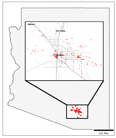
Figure 1: Clustering of buffelgrass observations in Arizona made by USA-NPN staff and volunteers.

for example, address the problem of buffelgrass site detection using UAVs and satellite imagery. Other prior work has also examined detecting unobserved buffelgrass sites using remote imagery, but does not explicitly model the readiness of those sites for herbicidal treatment [7, 2, 16].

Green-up prediction requires phenological observations. A primary source of observations is the USA National Phenology Network (USA-NPN), a national-scale monitoring and research initiative focused on collecting research-grade phenological data, information, and forecasts [4]. USA-NPN offers a “Buffelgrass Pheno Forecast,” which currently uses the baseline accumulated precipitation model based on thresholding [29] and forecasts 50% green up at 4km resolution across the state of Arizona [8]. Additionally, USA-NPN facilitates the collection of high-quality observations of plant and animal life cycle stages through Nature’s Notebook, a freely available phenology citizen science platform and dataset used by thousands of volunteer and professional scientists. Buffelgrass is one of over 1,700 species participants can observe at locations of their choosing [24].

3 Methodology

Datasets

We leverage three distinct sources of data. First, we use volunteer contributed buffelgrass phenology observations (e.g. green-up percentage $\geq\%50$) from hundreds of unique locations, gathered using USA-NPN’s Nature’s Notebook platform. Second, we gather climate data from ERA5-Land, which is a reanalysis dataset with 50 land variables spanning several decades [18]. Of these variables, we selected 16 variables for experimentation based on domain expertise; they are listed in Table 2 in the appendix. Third, we utilize satellite images provided by PlanetAPI, which offers higher-resolution (3.7 meters per pixel) than standard public domain satellite imagery like Sentinel. A more detailed dataset description as well as our training practices (hyper-parameters, data splits, etc.) can be found in Sections 6.2 and 6.3 respectively in the appendix.

Model 1: Accumulative Precipitation Baseline (AP) A standard, science-backed, heuristic method for predicting buffelgrass phenology, the Accumulative Precipitation model (AP) simply calculates the total amount of precipitation over the past 24 days [29]. If this accumulative precipitation exceeds 1.7 inches, buffelgrass is likely to have a greenness level exceeding 50%. This method is currently deployed by USA-NPN [8].

Model 2: Long Short Term Memory (LSTM) The AP model may fail to capture sequential long-term patterns or dependencies effectively, and does not incorporate other environmental variables directly [29]. We theorized that the LSTM [12] architecture would be well-suited for modeling the correlation between buffelgrass greenness and patterns in weather during the days leading up to observation, as LSTMs have been shown to be effective at modeling temporal patterns in climate data [23]. Our experiments use LSTMs with two different input sequences: LSTM (single) only utilizes a sequence of precipitation values as input, to be more directly comparable to the AP model. On the otherhand, LSTM (multi) takes input from a sequence of many external climate feature values in addition to precipitation values (listed in Table 2 in Appendix).

Figure 2: Four $90\times 90$ meter patches, each centered at a buffelgrass observation site.

Model 3: Vision Transformer (ViT) The Vision Transformer (ViT), as introduced in [6], is a model primarily designed for image classification tasks. It adopts a Transformer-like architecture that operates on image patches. In our work, we fine-tuned the pre-trained model google/vit-base-patch16-224-in21k using PlanetAPI data.

Model 4: Multi-Modal LSTM+ViT The LSTM models are designed to process sequential features, while the ViT model excels at making predictions based on spatial information derived from satellite images. Recognizing the potential for these two modalities to enhance each other’s performance when combined, we adopt a multi-modal approach, which has been shown to capture non-overlapping signal and improve climate models [13]. Specifically, we leverage the ViT model to generate embeddings from satellite images. These embeddings are then concatenated with the sequential embeddings derived from external features with LSTM. A final linear layer then yields predictions.

4 Results and Discussion

Neural Models Outperform Simple AP Model

The prediction results are presented in Table 1. Note that all of the neural models exhibit better performance compared to the simple accumulative precipitation model (AP). Explicitly modeling temporal precipitation patterns alone is enough for a significant boost, as even LSTM (single) demonstrates a notable enhancement in accuracy (13% points $\uparrow$), F1 (0.26 $\uparrow$) over the AP model. With added variables, the LSTM (multi) achieves the best accuracy, F1, and false negative rate of all models, with smaller standard deviations, underscoring the importance of temporal features and other climate variables in modeling this task.

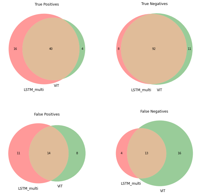
Figure 7: Understanding the overlapping correctness between our LSTM (multi) and ViT models informed our decision to pursue a multi-modal approach. Above, you can see the overlapping correctness for the two models, for each class in the confusion matrix. Though both models agree on at least a plurality of predictions in each case, their predictive correctness does not overlap entirely. In fact, the types of errors each model makes are vastly different, and suggests to us that non-overlapping signal might be captured by using an ensemble or multi-modal approach. Though we did not succeed in creating a multi-modal approach that fully utilized this signal, we believe that future improvements in green-up accuracy will be dependent on combining direct satellite observation with climate and other remote sensing data in this way.

The ViT model, relying solely on satellite imagery, also improves over AP in accuracy (6% points $\uparrow$), F1 (0.18 $\uparrow$), and false positive rate (7% $\downarrow$). Despite beating AP, the ViT model underperformed the LSTM models. We believe this is for two reasons: (1) the observation-date-only satellite imagery lacks necessary temporal features and (2) the quality of the satellite images matters, but varies among the images obtained from the PlanetAPI. At our current pixel resolution (1 pixel $\approx$ 3.7 meters), it is hard to detect the shapes and edges of buffelgrass (which often occurs in small clumps $<10\times 10$ meters), spatial features that are usually helpful in image classification tasks. Furthermore, some images are distorted by artifacts of the satellite collection process, containing pure random noise (e.g., white/black pixels). Combining both ViT and LSTM yields results that surpass ViT alone but fall slightly short of the performance achieved by LSTM (multi). Despite this, we are excited by the potential for multi-modal modeling in this domain – see Figures 7and 8 in the appendix for an in depth discussion. With higher quality satellite imagery (such as from the Pleiades mission) and full temporal cover (i.e. images for each day leading up to observation), we believe that multi-modal models will eventually outperform LSTM (multi). As it stands, this imagery is prohibitively expensive, but we hope to gain access to a higher volume and quality of satellite imagery in future project iterations.

Model	Accuracy	F1	FP	FN
AP	63.64% (0.00%)	0.36 (0.00)	26.77% (0.00%)	9.60% (0.00%)
LSTM (single)	76.57% (2.85%)	0.62 (0.06)	17.07% (3.29%)	6.36% (2.25%)
LSTM (multi.)	78.08% (1.91%)	0.73 (0.02)	6.97% (0.81%)	14.95% (2.20%)
ViT	69.90% (3.28%)	0.54 (0.06)	19.09% (3.29%)	11.01% (3.94%)
LSTM (multi) +ViT	75.66% (1.25%)	0.70 (0.02)	8.48% (2.00%)	15.86% (1.93%)

Table 1: Buffelgrass prediction performances. The accuracy, f1 score, false positive (FP) and false negative (FN) rates are reported. The 5-fold standard deviations are reported in the parenthesis.

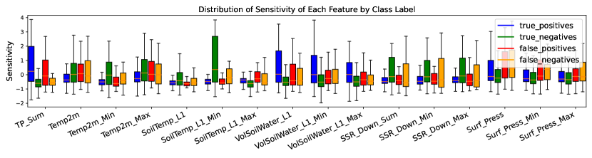
Figure 3: Aggregated sensitivities of LSTM (multi) across features, by confusion matrix classes. As expected, true positives are highly sensitive to TP_Sum, VolSoilWater_L1 – precipitation matters. Interestingly, true negatives are highly sensitive to Soil_Temp - we conjecture that sufficiently hot days preclude green-up even with precipitation. Table 3 has mapping of abbreviated feature names.

Feature Importance and Sensitivity Analysis

We analyze our highest performing model, LSTM (multi), with the caveat that neural networks are inherently difficult to interpret [33]. Our primary analysis centers on model sensitivity – procedural perturbations of training samples to elicit model behavior [26]. Informally, our sensitivity analysis goes as follows: (1) for model $M$ and for training sample $x$, determine mean value $\mu_{k}$ for feature $k$, (2) create $x^{\prime}$, which is a copy of $x$ where the value of feature $k$ in $x$ is set to $\mu_{k}$ (3) compute absolute difference $|M(x)-M(x^{\prime})|$. We split our data into classes based on the confusion matrix to further clarify patterns [25]. In Figures 4 and 5, we show complete sensitivity results on LSTM (multi). In Figure 3 we then aggregate and z-normalize results across all samples to look for global patterns; see Section 7 in the appendix for more analysis.

Resource Savings, Deployment and Impact

Many organizations use the USA-NPN’s Buffelgrass Pheno Forecast maps to shape treatment efforts, including Pima County and the US Forest Service. These organizations manage multiple geographically diverse properties spread across southern Arizona, and green-up prediction tools shape costly crew deployments on any given day.

Models like LSTM (multi) can dramatically improve crew deployment accuracy, specifically because they reduce false positive predictions over AP. False positives are especially problematic; situations where crews are dispatched to a location but the buffelgrass is not sufficiently green for treatment wastes hundreds of dollars in crew time and vehicle fuel [9]. False negatives are increased slightly by the neural based models, but that is more manageable because the window for herbicidal treatment (to prevent ripe seed production) is a few weeks. Model reruns with updated climate or imagery data would then still hope to turn false negatives into true positives as the phenocycle matures.

5 Conclusion

In this work, we tackle the problem of predicting the greenness of buffelgrass, aiming to reduce wildfire risk and protect biodiversity. We construct deep neural models that can leverage temporal information from climate features and spatial information from satellite images. Our experimental results show that: (1) neural models improve significantly over the currently deployed heuristic prediction models and (2) LSTMs with temporal climate features had the strongest predictive power of the models we tested. As satellite imagery coverage and resolution improves, one day we hope to deploy indirect climate based models alongside direct observation of greenness. For now, climate based LSTM models offer strong performance and smooth daily implementation; they are a new standard in buffelgrass green-up prediction models.

6 Appendix

6.1 External Variables

Variable	Definition
total_precipitation_sum	Accumulated liquid and frozen water, including rain and snow, that falls to the Earth’s surface.
temperature_2m	Temperature of air at 2m above the surface of land, sea or in-land waters.
temperature_2m_min	daily minimum temperature_2m value
temperature_2m_max	daily maximum temperature_2m value
soil_temperature_level_1	Temperature of the soil in layer 1 (0 - 7 cm) of the ECMWF Integrated Forecasting System.
soil_temperature_level_1_min	daily minimum soil_temperature_level_1 value
soil_temperature_level_1_max	daily maximum soil_temperature_level_1 value
volumetric_soil_water_layer_1	Volume of water in soil layer 1 (0 - 7 cm) of the ECMWF Integrated Forecasting System.
volumetric_soil_water_layer_1_min	daily minimum volumetric_soil_water_layer_1 value
volumetric_soil_water_layer_1_max	daily maximum volumetric_soil_water_layer_1 value
surface_solar_radiation_downwards_sum	Amount of solar radiation (also known as shortwave radiation) reaching the surface of the Earth.
surface_solar_radiation_downwards_min	daily minimum surface_solar_radiation_downwards_sum value
surface_solar_radiation_downwards_max	daily maximum surface_solar_radiation_downwards_sum value
surface_pressure	Pressure (force per unit area) of the atmosphere on the surface of land, sea and in-land water.
surface_pressure_min	daily minimum surface_pressure value
surface_pressure_max	daily maximum surface_pressure value

Table 2: External features for buffelgrass greenness prediction.

Original Feature Name	Abbreviated Name
total_precipitation_sum	TP_Sum
temperature_2m	Temp2m
temperature_2m_min	Temp2m_Min
temperature_2m_max	Temp2m_Max
soil_temperature_level_1	SoilTemp_L1
soil_temperature_level_1_min	SoilTemp_L1_Min
soil_temperature_level_1_max	SoilTemp_L1_Max
volumetric_soil_water_layer_1	VolSoilWater_L1
volumetric_soil_water_layer_1_min	VolSoilWater_L1_Min
volumetric_soil_water_layer_1_max	VolSoilWater_L1_Max
surface_solar_radiation_downwards_sum	SSR_Down_Sum
surface_solar_radiation_downwards_min	SSR_Down_Min
surface_solar_radiation_downwards_max	SSR_Down_Max
surface_pressure	Surf_Press
surface_pressure_min	Surf_Press_Min
surface_pressure_max	Surf_Press_Max

Table 3: Mapping of original feature names to abbreviated names.

6.2 Datasets

Prediction Data: Our phenological prediction data actually comprises data from two similar sources:

• Nature’s Notebook Observation Data: Volunteer participants have contributed buffelgrass phenology observations at hundreds of unique locations using the USA-NPN’s Nature’s Notebook platform. Nature’s Notebook is designed to encourage repeated observations on the same individual plants over the growing season, ideally capturing green-up, flowering, seed ripening, and senescence. Individual observations consist of observation location (longitude and latitude), elevation, phenological status (whether the plant is green or not; whether the plant is flowering or not; whether fruits are present; etc.) as well as the intensity or abundance of present phenophases (if the plant is green, how much of the plant is green?) on a single date. The nature’s notebook observations include 1,698 distinct $location\times date$ observations in total. According to standard practices described in Gerst et al. [8], we reclassified greenness reports observations as: 1 if greenness exceeds 50%; 0 otherwise.

• Local One-Time Observation Data: Because buffelgrass is highly invasive, the plants are often removed when observed, rendering repeated phenological observations within the Nature’s Notebook platform impossible. Accordingly, in 2019, the USA-NPN created an online form through which professionals and volunteers treating buffelgrass could report the instantaneous phenological status of buffelgrass plants. These “one-time” observations are primarily used by the USA-NPN to validate existing Pheno Forecast maps. The format of this data matches Nature’s Notebook observations, and we follow the same greenness reclassifying procedure, providing us with an additional 194 observations.

Google Earth — ERA5-Land Data: To improve predictions, we use external climate or weather features that may correlate with buffelgrass greenness. ERA5-Land is a reanalysis dataset that furnishes data on 50 land variables spanning several decades at a higher resolution than the original ERA5 dataset [18]. For more comprehensive information regarding this dataset, readers are directed to [19]. For each entry in the Nature’s Notebook dataset, we obtain external feature values from a period starting at the observation date and extending back 24 days. We have selected 16 variables for experimentation, and these are listed in Table 2.

Planet Satellite Images: As discussed, several studies [22, 7] have previously employed satellite imagery to detect the presence of buffelgrass. In contrast, our research focuses on a different task, which is to predict the greenness of buffelgrass using high-resolution satellite images. To facilitate this endeavor, we utilize high-resolution satellite images provided by Planet , which offer a resolution of 3.7 meters. For each data record, we extract satellite images centered around the observation location point, corresponding to the observation date. Each image has the dimension of $369\times 369$.

6.3 Training

By combining all our prediction data sources, we were left with 987 observations to experiment with (some observations did not have accompanying satellite imagery from PlanetAPI, as they predate the launch of the mission in 2016). We initially divided the 987 observations into a training set comprising 798 observations and a test set consisting of 198 observations. We then conducted a 5-fold cross-validation procedure on the training set to develop our models. To gauge the variability in model performance, we calculated the standard deviation across the 5 folds.

For the AP model, there is no training needed. For the LSTM models, they are composed of two LSTM layers with a hidden dimension of 128, and a linear layer for prediction. During training, the batch size is set to 4, the learning rate to 1e-4, and the number of training epochs to 500. The ViT model is trained with a batch size of 2, a learning rate of $1e-5$, and it undergoes 10 training epochs. The LSTM+ViT model is trained with a batch size of 4, a learning rate of $1e-5$ for 100 training epochs. In all cases, a consistent random seed of 816 is employed for model training to ensure reproducibility and consistency in results.

7 Sensitivity Analysis

Below we provide sensitivty analysis figures for LSTM (multi) across every feature. Every point in each plot represents a sample in our training data, and is color coded by the confusion matrix class of the prediction that sample received by the LSTM (multi) model. You may immediately note that the LSTM (multi) model does not produce calibrated predictions i.e. the predictions are not true probabilities $\in[0,1]$, though we do threshold by 0.5. In our case, we found that taking extra steps to calibrate the model reduced model performance, which is common for deep learning models and complex architectures [11]. Thus, it is better to think of the model outputs as likelihood scores.

Here we take a close look at each plot in order, to ascertain feature specific patterns. Note that we will delineate between sensitivity observations and conjectures about root causes.

• In Figure 4(a), we look at the Total Precipitation Sum. This is accumulated liquid and frozen water like rain and snow, stemming from both large-scale weather patterns and convective activities, measured in depth (meters) and representing the depth water would have if spread evenly over a grid box. We note the upward trend in sensitivity among the true positive class (in blue) as the model predictions get higher. This suggests that higher likelihood green-ups (i.e. higher model predictions) are especially sensitive to reduced precipitation to the mean.

• In Figures 4(b), 4(c) and 4(d), we examine Temperature (2 meters), as well as Max and Min Temperature (2 meters) respectively. This is air temperature calculated 2 meters above the surface of land, sea, or inland waters, modeled considering atmospheric conditions. These are highly correlated features and thus the trends in their sensitivity are similar: true negative samples are the most highly sensitive samples to this class. As temperature is correlated with precipitation and moisture levels, we conjecture that higher temperatures imply more certainty about no green-up. We further note that this feature had the smallest effects in aggregate on model predictions (see Figure 6).

• In Figures 4(e), 4(f) and 4(g), we analyze the sensitivity of Solar Radiation Downward Sum, Max and Min respectively. This represents the amount of solar radiation, including both direct and diffuse, reaching the Earth’s surface, accounting for reflection by clouds and aerosols and absorption, approximating what would be measured by a pyranometer. Similarly to temperature, this variable is correlated with precipitation (sun implies no cloud cover, which implies less moisture). Based on the sensitivity plot, we conjecture that the model primarily used this variable in determining true negatives.

• In Figures 5(a), 5(b) and 5(c), we observe sensitivity of Surface Pressure, Max and Min respectively. This pressure variable, measured in Pascals (Pa), represents the atmospheric pressure on the surface of land, sea, and inland water, reflecting the weight of the air column above, and is utilized alongside temperature to determine air density, with mean sea level pressure commonly used for identifying pressure systems over mountainous areas. We were surprised by the sensitivity of the model to this variable. However, it is known that surface pressure is heavily correlated with weather systems, and can independently effect the rate of plant photosynthesis through disruptions to transpiration [27]. Still, we found it difficult to interpret the effects of this variable, particularly with respect to false positives and false negatives. We worry that it could be confounding, and may remove it in future model iterations.

• In Figures 5(d), 5(e) and 5(f), we study the sensitivity of Soil Temperature (Level 1), Max and Min respectively. The temperature of soil in layer 1 (0 - 7 cm) is set at the middle of each layer, with heat transfer calculated at the interfaces between them, and an assumption of no heat transfer out of the bottom of the lowest layer. Most samples were not particularly sensitive to this variable, where others were. The sensitivities suggests that the max soil temperature was useful in deciding positive classifications, while the min soil temperature was useful in negative classifications. The soil temperature likely correlates with water volume and solar heat, which partially explains the sensitivities.

• In Figure 5(g), 5(h) and 5(i), the Volumetric Soil Water (Layer 1), Max and Min is examined. The volumetric soil water in soil layer 1 (0 - 7 cm) is related to the soil texture, depth, and the underlying groundwater level, with the surface at 0 cm. Soil water is vital for plant growth and thus for accurate positive predictions - an upward trend in model likelihood scores correlated with higher sensitivity is apparent in all three sensitivity plots.

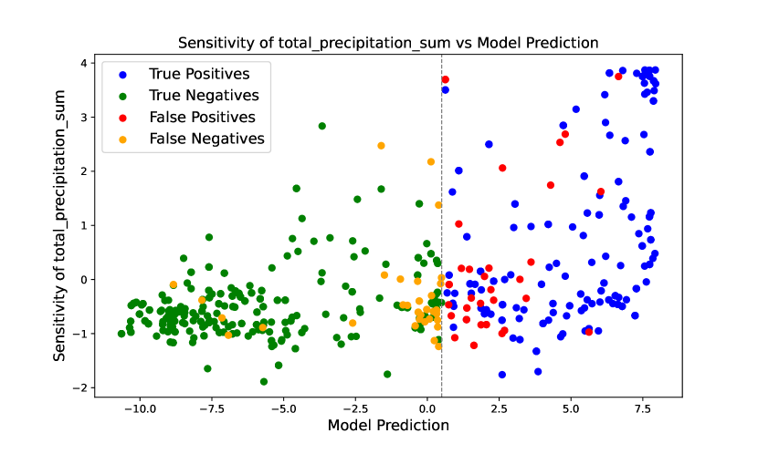
(a) Total Precipitation Sum

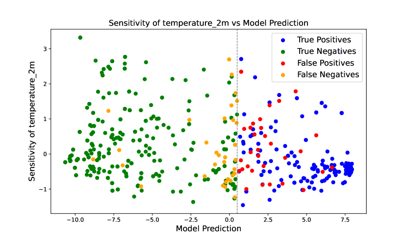
(b) Temperature (2m)

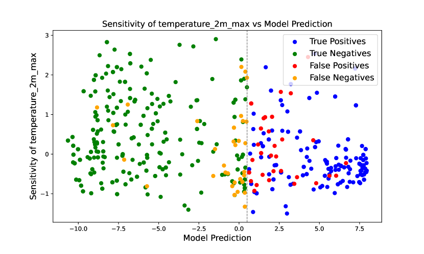
(c) Temperature (2m) Max

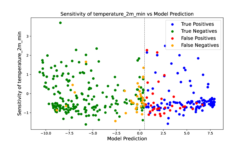
(d) Temperature (2m) Min

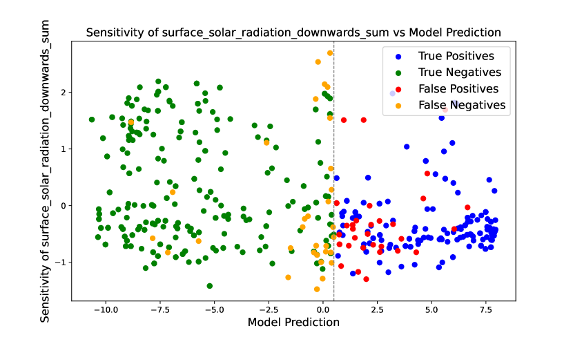
(e) Solar Radiation Downward Sum

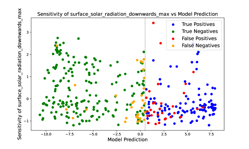
(f) Solar Radiation Downward Max

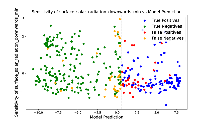
(g) Solar Radiation Downward Min

Figure 4: Sensitivity Plots

Figure 5: Sensitivity Plots

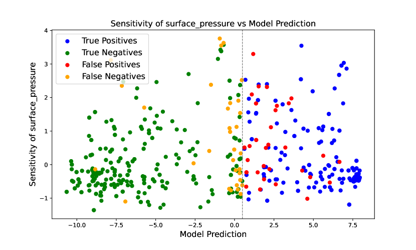
(a) Surface Pressure

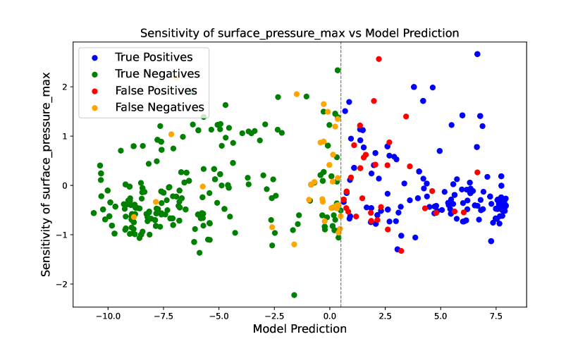
(b) Surface Pressure Max

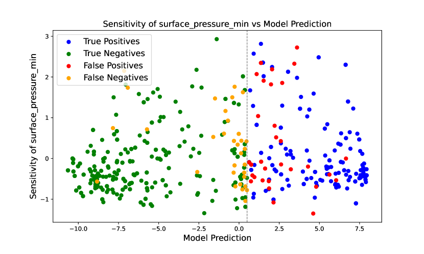
(c) Surface Pressure Min

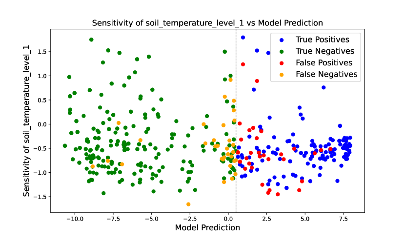
(d) Soil Temperature Level 1

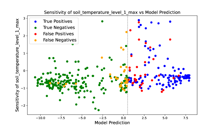
(e) Soil Temperature Level 1 Max

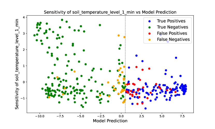
(f) Soil Temperature Level 1 Min

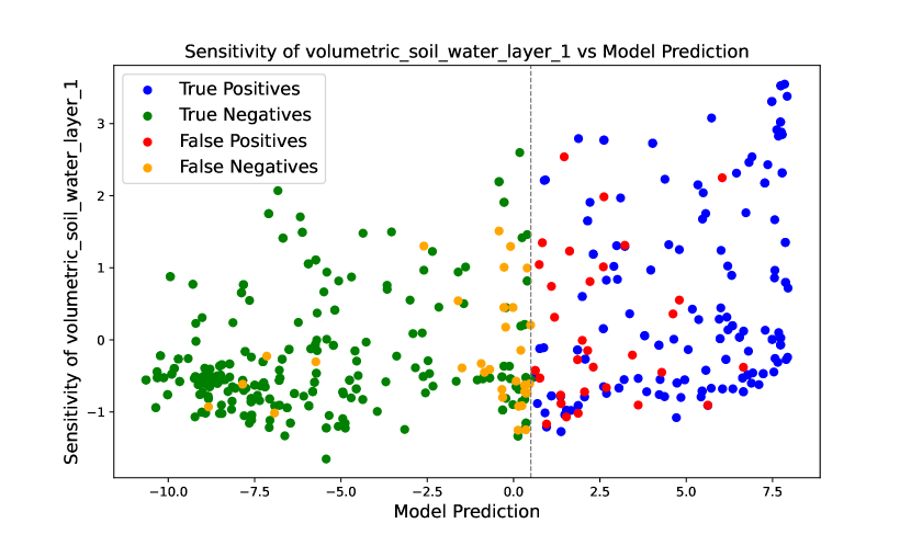
(g) Volumetric Soil Water Layer 1

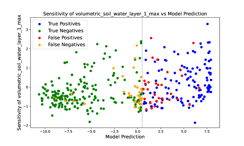
(h) Volumetric Soil Water Layer 1 Max

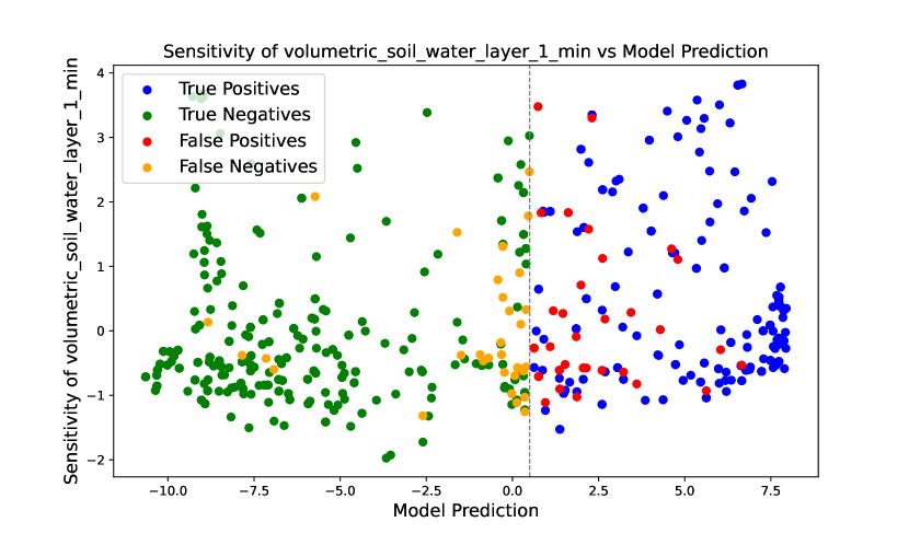
(i) Volumetric Soil Water Layer 1 Min

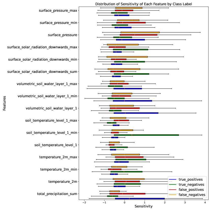
Figure 6: This plot replicates Figure 3, but vertically, allowing for ease of reading.

(a) LSTM Unique True Positives (ViT False Negatives).

(b) ViT Unique True Positives (LSTM False Negatives).

(c) LSTM Unique True Negatives (ViT False Positives).

(d) ViT Unique True Negatives (LSTM False Positives).

Figure 8: To provide a sense of the types of mistakes the ViT model makes in particular, we provide the following patches of satellite imagery, corresponding to confusion matrix sections of the Venn diagram in Figure 7. You can see that images the ViT model “missed” (i.e. false negatives) in relation to the LSTM (multi) model are almost entirely due to poor image quality or cloud cover. Meanwhile, unique LSTM true negatives and unique ViT true positives have similar image quality, suggesting the model is inherently biased towards higher quality images for positive classification. This type of bias would be ameliorated through the collection of more data and better image cleaning procedures, as well as higher resolution imagery.

References

- Agriculture Department [2017] Forest Service Agriculture Department. Field guide for managing buffelgrass in the southwest. https://www.govinfo.gov/app/details/GOVPUB-A13-PURL-gpo89749, 2017. [Accessed 24-09-2023].
- Brenner et al. [2012] Jacob C Brenner, Zachary Christman, and John Rogan. Segmentation of landsat thematic mapper imagery improves buffelgrass (pennisetum ciliare) pasture mapping in the sonoran desert of mexico. Applied Geography, 34:569–575, 2012.
- Canon [2022] Gabrielle Canon. “turning the dial up”: Us south-west braces for extended wildfire season amid drastic drought, May 2022. URL https://www.theguardian.com/world/2022/may/01/us-new-mexico-drought-wildfire-southwest.
- Crimmins et al. [2022] Theresa Crimmins, Ellen Denny, Erin Posthumus, Alyssa Rosemartin, Rob Croll, Melonee Montano, and Hannah Panci. Science and management advancements made possible by the usa national phenology network’s nature’s notebook platform. BioScience, 72(9):908–920, 2022.
- de Albuquerque et al. [2019] Fábio Suzart de Albuquerque, Miguel Ángel Macías-Rodríguez, Alberto Búrquez, and Yaiyr Astudillo-Scalia. Climate change and the potential expansion of buffelgrass (cenchrus ciliaris l., poaceae) in biotic communities of southwest united states and northern mexico. Biological Invasions, 21:3335 – 3347, 2019. URL https://api.semanticscholar.org/CorpusID:195796162.
- Dosovitskiy et al. [2020] Alexey Dosovitskiy, Lucas Beyer, Alexander Kolesnikov, Dirk Weissenborn, Xiaohua Zhai, Thomas Unterthiner, Mostafa Dehghani, Matthias Minderer, Georg Heigold, Sylvain Gelly, et al. An image is worth 16x16 words: Transformers for image recognition at scale. arXiv preprint arXiv:2010.11929, 2020.
- Elkind et al. [2019] Kaitlyn Elkind, Temuulen T Sankey, Seth M Munson, and Clare E Aslan. Invasive buffelgrass detection using high-resolution satellite and uav imagery on google earth engine. Remote Sensing in Ecology and Conservation, 5(4):318–331, 2019.
- Gerst et al. [2021] Katharine L Gerst, Theresa M Crimmins, Erin Posthumus, R Lee Marsh, Jeff Switzer, and Cynthia Wallace. The usa national phenology network’s buffelgrass green-up forecast map products. Ecological Solutions and Evidence, 2(4):e12109, 2021.
- Grissom [2019] Perry Grissom. Buffelgrass facts and figures. Saguaro National Park Service, 2019. URL https://www.nps.gov/sagu/learn/nature/upload/BG-facts-and-figures-Aug-2019.pdf.
- Grissom [2022] Perry Grissom. “share protecting and restoring the sonoran desert ecosystem in saguaro national park, 2022. URL https://www.doi.gov/wildlandfire/news/protecting-and-restoring-sonoran-desert-ecosystem-saguaro-national-park.
- Guo et al. [2017] Chuan Guo, Geoff Pleiss, Yu Sun, and Kilian Q Weinberger. On calibration of modern neural networks. In International conference on machine learning, pages 1321–1330. PMLR, 2017.
- Hochreiter and Schmidhuber [1997] Sepp Hochreiter and Jürgen Schmidhuber. Long short-term memory. Neural computation, 9(8):1735–1780, 1997.
- Hong et al. [2020] Danfeng Hong, Lianru Gao, Naoto Yokoya, Jing Yao, Jocelyn Chanussot, Qian Du, and Bing Zhang. More diverse means better: Multimodal deep learning meets remote-sensing imagery classification. IEEE Transactions on Geoscience and Remote Sensing, 59(5):4340–4354, 2020.
- Li et al. [2023] Yue M Li, Seth M Munson, Ya-Ching Lin, and Perry Grissom. Effectiveness of a decade of treatments to reduce invasive buffelgrass (pennisetum ciliare). Invasive Plant Science and Management, 16(1):27–37, 2023.
- Marshall et al. [2012] VM Marshall, MM Lewis, and B Ostendorf. Buffel grass (cenchrus ciliaris) as an invader and threat to biodiversity in arid environments: a review. Journal of Arid Environments, 78:1–12, 2012.
- Marshall et al. [2014] VM Marshall, MM Lewis, and B Ostendorf. Detecting new buffel grass infestations in australian arid lands: evaluation of methods using high-resolution multispectral imagery and aerial photography. Environmental monitoring and assessment, 186:1689–1703, 2014.
- McDonald and McPherson [2013] Christopher J McDonald and Guy R McPherson. Creating hotter fires in the sonoran desert: Buffelgrass produces copious fuels and high fire temperatures. Fire Ecology, 9:26–39, 2013.
- Muñoz-Sabater et al. [2021] Joaquín Muñoz-Sabater, Emanuel Dutra, Anna Agustí-Panareda, Clément Albergel, Gabriele Arduini, Gianpaolo Balsamo, Souhail Boussetta, Margarita Choulga, Shaun Harrigan, Hans Hersbach, et al. Era5-land: A state-of-the-art global reanalysis dataset for land applications. Earth system science data, 13(9):4349–4383, 2021.
- Muñoz Sabater et al. [2021] Joaquín Muñoz Sabater, Emanuel Dutra, Anna Agusti-Panareda, Clement Albergel, Gabriele Arduini, Gianpaolo Balsamo, Souhail Boussetta, Margarita Choulga, Shaun Harrigan, Hans Hersbach, Brecht Martens, Diego Miralles, Maria Piles, Nemesio Rodriguez-Fernandez, Ervin Zsótér, Carlo Buontempo, and J.-N Thépaut. Era5-land: A state-of-the-art global reanalysis dataset for land applications, 03 2021.
- Nolan et al. [2022] Rachael H Nolan, Liana O Anderson, Benjamin Poulter, and J Morgan Varner. Increasing threat of wildfires: the year 2020 in perspective: A global ecology and biogeography special issue. Global Ecology and Biogeography, 31(10):1898–1905, 2022.
- Olsson et al. [2012] Aaryn D Olsson, Julio L Betancourt, Michael A Crimmins, and Stuart E Marsh. Constancy of local spread rates for buffelgrass (pennisetum ciliare l.) in the arizona upland of the sonoran desert. Journal of Arid Environments, 87:136–143, 2012.
- Papp et al. [2021] Levente Papp, Boudewijn Van Leeuwen, Péter Szilassi, Zalán Tobak, Jozsef Szatmari, Mátyás Árvai, János Mészáros, and László Pásztor. Monitoring invasive plant species using hyperspectral remote sensing data. Land, 10, 01 2021. doi: 10.3390/land10010029.
- Park et al. [2020] Sumin Park, Jungho Im, Daehyeon Han, and Jinyoung Rhee. Short-term forecasting of satellite-based drought indices using their temporal patterns and numerical model output. Remote Sensing, 12(21):3499, 2020.
- Rosemartin et al. [2014] Alyssa H Rosemartin, Theresa M Crimmins, Carolyn AF Enquist, Katharine L Gerst, Jherime L Kellermann, Erin E Posthumus, Ellen G Denny, Patricia Guertin, Lee Marsh, and Jake F Weltzin. Organizing phenological data resources to inform natural resource conservation. Biological Conservation, 173:90–97, 2014.
- Shen et al. [2020] Hong Shen, Haojian Jin, Ángel Alexander Cabrera, Adam Perer, Haiyi Zhu, and Jason I Hong. Designing alternative representations of confusion matrices to support non-expert public understanding of algorithm performance. Proceedings of the ACM on Human-Computer Interaction, 4(CSCW2):1–22, 2020.
- Shu and Zhu [2019] Hai Shu and Hongtu Zhu. Sensitivity analysis of deep neural networks. In Proceedings of the AAAI Conference on Artificial Intelligence, volume 33, pages 4943–4950, 2019.
- Takeishi et al. [2013] Hiroyuki Takeishi, Jun Hayashi, Atsushi Okazawa, Kazuo Harada, Kazumasa Hirata, Akio Kobayashi, and Fumiteru Akamatsu. Effects of elevated pressure on rate of photosynthesis during plant growth. Journal of biotechnology, 168(2):135–141, 2013.
- Wallace et al. [2014] Cynthia Wallace, Jake F Weltzin, Susan M Skirvin, Caroline Patrick-Birdwell, and Helen Raichle. Predicting treatment windows for invasive buffelgrass in southern arizona using modis and climate data. In AGU Fall Meeting Abstracts, volume 2014, pages B41K–0204, 2014.
- Wallace et al. [2016] Cynthia Wallace, Jessica Walker, Susan Skirvin, Caroline Patrick-Birdwell, Jake Weltzin, and Helen Raichle. Mapping presence and predicting phenological status of invasive buffelgrass in southern arizona using modis, climate and citizen science observation data. Remote Sensing, 8:524, 06 2016. doi: 10.3390/rs8070524.
- Wayne Hanselka et al. [2004] C Wayne Hanselka, Mark A Hussey, and Ibarra F Fernando. Buffelgrass. Warm-Season (C4) Grasses, 45:477–502, 2004.
- Wilder et al. [2021] Benjamin T Wilder, Catherine S Jarnevich, Elizabeth Baldwin, Joseph S Black, Kim A Franklin, Perry Grissom, Katherine A Hovanes, Aaryn Olsson, Jim Malusa, Abu SMG Kibria, et al. Grassification and fast-evolving fire connectivity and risk in the sonoran desert, united states. Frontiers in Ecology and Evolution, 9:655561, 2021.
- Williams et al. [2019] A Park Williams, John T Abatzoglou, Alexander Gershunov, Janin Guzman-Morales, Daniel A Bishop, Jennifer K Balch, and Dennis P Lettenmaier. Observed impacts of anthropogenic climate change on wildfire in california. Earth’s Future, 7(8):892–910, 2019.
- Zhang et al. [2021] Yu Zhang, Peter Tiňo, Aleš Leonardis, and Ke Tang. A survey on neural network interpretability. IEEE Transactions on Emerging Topics in Computational Intelligence, 5(5):726–742, 2021.
- Zhao et al. [2021] Qiang Zhao, Le Yu, Xuecao Li, Dailiang Peng, Yongguang Zhang, and Peng Gong. Progress and trends in the application of google earth and google earth engine. Remote Sensing, 13(18):3778, 2021.