EventLFM: Event Camera integrated Fourier Light Field Microscopy for Ultrafast 3D imaging

Ruipeng Guo\authormark1 Qianwan Yang\authormark1 Andrew S. Chang\authormark4 Guorong Hu\authormark1 Joseph Greene\authormark1 Christopher V. Gabel\authormark3,4 Sixian You\authormark5 and Lei Tian\authormark1,2,3 \authormark1Department of Electrical and Computer Engineering, Boston University, Boston, MA 02215, USA.
\authormark2Department of Biomedical Engineering, Boston University, Boston, MA 02215, USA.
\authormark3Neurophotonics Center, Boston University, Boston, MA 02215, USA.
\authormark4Department of Physiology and Biophysics, Boston University, Boston, MA 02215, USA.
\authormark5Research Laboratory of Electronics (RLE) in the Department of Electrical Science and Engineering, Massachusetts Institute of Technology, Cambridge, MA 02139, USA. \authormark*leitian@bu.edu

Abstract

Ultrafast 3D imaging is indispensable for visualizing complex and dynamic biological processes. Conventional scanning-based techniques necessitate an inherent trade-off between acquisition speed and space-bandwidth product (SBP). Emerging single-shot 3D wide-field techniques offer a promising alternative but are bottlenecked by the synchronous readout constraints of conventional CMOS systems, thus restricting data throughput to maintain high SBP at limited frame rates. To address this, we introduce EventLFM, a straightforward and cost-effective system that overcomes these challenges by integrating an event camera with Fourier light field microscopy (LFM), a state-of-the-art single-shot 3D wide-field imaging technique. The event camera operates on a novel asynchronous readout architecture, thereby bypassing the frame rate limitations inherent to conventional CMOS systems. We further develop a simple and robust event-driven LFM reconstruction algorithm that can reliably reconstruct 3D dynamics from the unique spatiotemporal measurements captured by EventLFM. Experimental results demonstrate that EventLFM can robustly reconstruct fast-moving and rapidly blinking 3D samples at kHz frame rates. Furthermore, we highlight EventLFM’s capability for imaging of blinking neuronal signals in scattering mouse brain tissues and 3D tracking of GFP-labeled neurons in freely moving C. elegans. We believe that the combined ultrafast speed and large 3D SBP offered by EventLFM may open up new possibilities across many biomedical applications.

^†^†journal: opticajournal^†^†articletype: Research Article

1 Introduction

High-speed volumetric imaging is an indispensable tool for investigating dynamic biological processes[1]. Traditional scanning-based 3D imaging techniques such as confocal microscopy[2], two-photon microscopy[3] and light-sheet microscopy[4] offer high spatial resolution. However, their data acquisition speeds are often constrained by the need for beam scanning. Consequently, these techniques suffer from an inherent trade-off between temporal resolution and the space-bandwidth product (SBP), measured by the ratio of the 3D field-of-view (FOV) to the spatial resolution.

Single-shot 3D widefield imaging techniques circumvent this trade-off by computational imaging. These methods first encode 3D information into 2D multiplexed measurements and then reconstruct the 3D volume computationally. Examples of such techniques include light field microscopy (LFM)[5, 6, 7, 8, 9], lensless imaging[10, 11, 12], and point-spread-function (PSF) engineering[13, 14]. Conventional LFM works by inserting a microlens array (MLA) into the native image plane of a widefield microscope[5]. Each microlens captures unique spatial and angular information from a sample, allowing for subsequent computational 3D reconstructions without scanning. However, this configuration suffers from intrinsic limitations, such as inconsistent spatial resolution due to uneven spatial sampling across the MLA. Recently, Fourier LFM has emerged as a solution to alleviate the limitations of the conventional LFM by positioning the MLA at the Fourier or pupil plane of a microscope[6, 7]. By recording the light field information at the Fourier domain, Fourier LFM ensures uniform angular sampling, which allows the technique to achieve a consistently high spatial resolution across the recovered volume. Despite these advancements, the synchronous readout constraints of traditional CMOS cameras remain a fundamental bottleneck for single-shot 3D wide-field techniques. Although it is possible to increase the frame rate by restricting the readout to only a specific region of interest (ROI) from the CMOS sensor, this inevitably results in a reduced SBP. As a result, existing LFM techniques typically operated below 100 Hz at the full-frame resolution. This constraint hinders their applications in capturing ultrafast dynamic biological processes that may exceed kilohertz (kHz), such as voltage signals in mammalian brains[15], blood flow dynamics[16] and muscle tissue contraction[17], thus leaving a significant technological gap yet to be bridged.

Refer to caption — Figure 1: Overview of EventLFM. (a) Schematics of the setup. (b) Space-time event spike stream captured by the event camera, where blue and red indicate negative and positive intensity changes at individual pixels, respectively. (c) Frames generated from the raw event stream using the time surface algorithm within a 1 ms accumulation time interval. (d) Depth color-coded 3D light field reconstruction of the object. (e) Time color-coded 3D motion trajectory reconstructed over a 45 ms time span.

To address these technological limitations, ultrafast imaging strategies have emerged, showing promise in various applications, such as characterization of ultrafast optical phenomena[18, 19], fluorescence lifetime imaging[20, 21], non-line-of-sight imaging[22], voltage imaging in mouse brains[23, 24, 25], and neurovascular dynamics recording[26]. Despite their merits, these techniques often come with their own trade-offs, such as the need for high-power illumination, which can be phototoxic to live biological specimens, and the need for expensive, specialized, and complicated optical systems.

Recently, event cameras have garnered significant attention over the past decade for their capability to provide kHz or higher frame rates while offering flexible integration into various platforms[27]. Unlike traditional CMOS cameras that record information from the full frame synchronously and at set time intervals, the event camera employs an asynchronous readout architecture. Each pixel on the event camera independently generates “event” readouts based on the changes in the pixel-level brightness over time. Each event recording contains information about the pixel’s position, timestamp, and polarity of the brightness change, allowing for ultra-high temporal resolution and reduced latency[28]. As a result, event camera enables recording of ultrafast signal changes at speeds exceeding 10 kHz limited only by pixel latency. In addition, event cameras are implicitly sensitive to changes in the logarithm of the photocurrent, allowing them to achieve high dynamic range that exceeds 120dB[29]. Leveraging these unique attributes, event cameras have shown promise across diverse applications, ranging from self-driving[30] and gesture recognition[31] to single-molecule localization microscopy[32, 33].

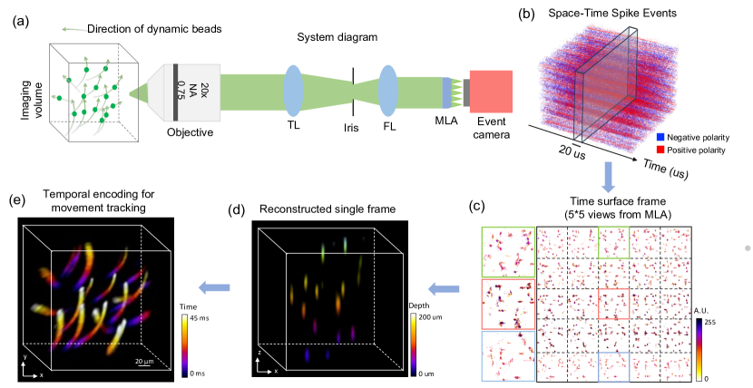
In this work, we introduce EventLFM, a novel ultrafast, single-shot 3D imaging technique that integrates an event camera into a Fourier LFM system, as illustrated in Fig. 1(a). We develop a simple event-driven LFM reconstruction algorithm to reliably reconstruct 3D dynamics from EventLFM’s spatiotemporal measurements. We experimentally demonstrate the applicability of EventLFM for 3D fluorescence imaging on various samples, achieving speeds of up to 1 kHz, effectively bridging the existing technological gaps in capturing ultrafast dynamic 3D processes.

To elucidate the method, Fig. 1 shows an example involving a suspension of fluorescent beads that traverse various trajectories within a 3D space. EventLFM captures a stream of events, as depicted in Fig. 1(b), which arise from instantaneous changes in intensity due to the rapid displacement of these beads across the FOV. Our event-driven LFM reconstruction algorithm works by first converting the acquired events into “conventional” 2D frame-based representations. This conversion is performed through a time-surface based method that leverages both spatial and temporal correlations among events over a predefined temporal-spatial window[34, 35]. The algorithm assigns values to each pixel based on accumulated historical data, which is shown in Fig. 1(c). Subsequently, these generated time-surfaces undergo processing via a light field refocusing algorithm[36], resulting in a 3D reconstruction. A representative frame depicting the 3D reconstruction of the fluorescent beads is provided in Fig.1(d) displaying with a depth color-coded map. Finally, to encapsulate the entire 4D information, a spatiotemporal reconstruction is visualized. This entails performing EventLFM reconstruction from the event measurements with an equivalent 1 kHz frame rate, spanned across a 45 ms time window. Figure 1(e) shows the recovered 3D trajectories of the fast-moving fluorescent beads with a depth color-coded map encoding the temporal information.

We provide a quantitative evaluation of EventLFM’s 4D imaging capabilities across a range of fast dynamic samples. This includes fast-moving fluorescent beads subjected to both controlled and random 3D motions, as well as rapid blinking beads that operate at frequencies up to 1 kHz, both with and without 3D motions. In addition, we showcase demonstrative bio-imaging experiments on the imaging of blinking neuronal signals simulated using a pulsed illumination in a 75 µm thick scattering mouse brain section and 3D tracking of labeled neurons in multiple freely moving C. elegans. Our results collectively demonstrate the robust and ultrafast 3D imaging capabilities of EventLFM, thereby underscoring its potential for elucidating intricate 3D dynamical phenomena within biological systems.

2 Methods

2.1 Experimental setup

EventLFM augments a conventional Fourier LFM setup with an event camera (EVK4, Prophesee), as shown in Fig. 1(a). A blue LED (SOLIS-1D, Thorlabs) serves as the excitation illumination source for the fluorescent samples. This excitation light is focused onto the back pupil plane of the objective lens (Plan Apo, 20 $\times$ , 0.75 NA, Nikon) to ensure uniform illumination across the target volume. In the detection path, fluorescence emissions from the sample are collected by the objective lens and subsequently relayed to an intermediate image plane by a tube lens (TL, $f$ = 200 mm, ITL200, Thorlabs). This intermediate image is then transformed by a Fourier lens (FL, $f$ = 80 mm, AC508-080-A, Thorlabs). An MLA ( $f$ = 16.8 mm, S600-f28, RPC Photonics) is placed at the back focal plane of the FL to achieve uniform angular sampling, thereby generating a 5 $\times$ 5 subimage array. An ancillary 4f relay system ( $M$ = 1.25, not shown) is placed after the MLA to ensure optimal distribution of these subimages across the event camera sensor. In addition, a 50/50 beamsplitter is integrated within the 4f system to enable simultaneous capture of the dynamic 3D volumes by both the event camera and an sCMOS camera (CS2100M-USB, Thorlabs), thereby providing a direct comparative benchmark between EventLFM and traditional Fourier LFM modalities. Further details can be found in Section 1 of Supplement 1.

2.2 Reconstruction algorithm

The event camera records the polarity of changes in pixel intensity as an event stream with a temporal granularity as fine as 1 $\mu$ s. Specifically, an event is generated when a dynamic or luminous variation within the FOV surpasses a pre-defined threshold. For each event, the sensor outputs the spatial coordinate $x$ and $y$ , the precise timestamp $t$ , and the polarity $p$ (either positive or negative depending on the direction of the intensity change). This asynchronous event stream is then sorted based on the polarity and integrated within a user-defined accumulation time to construct temporally continuous frames, as shown in Fig. 1(b). Our sensor has a pixel latency of 100 $\mu$ s - 220 $\mu$ s, setting the upper limit for accumulation time. To ensure a sufficient number of events for robust frame reconstruction, we set this time window between 1 to 2 milliseconds based on the specific sample under investigation. Importantly, the chosen accumulation time directly determines the system’s frame rate while also affecting the reconstruction resolution, details of which are elaborated in Section 3.

Rather than simply summing the events within the accumulation period, we apply a built-in time-surface algorithm for the post-processing of the raw event data. This algorithm employs an exponential time-decay function to compute a time surface, encapsulating both the spatial and temporal correlations among adjacent pixels. Pixel values in this time surface, ranging from 0 to 255, are indicative of historical temporal activity, as illustrated in Fig. 1(c). This approach offers a spatiotemporal representation for each event while mitigating motion blur artifacts (see Section 2 of Supplement 1 for details). Subsequently, these time-surface frames are processed by a standard light field refocusing algorithm[36] to yield a 3D volumetric reconstruction. To enhance the quality of the reconstruction, we apply a predefined threshold to remove ghosting artifacts introduced by the refocusing algorithm, as illustrated in Fig. 1(d). For visualization, we opt for either depth- or time-encoding color schemes when appropriate, as in Fig. 1(d) and 1(e).

2.3 System characterization

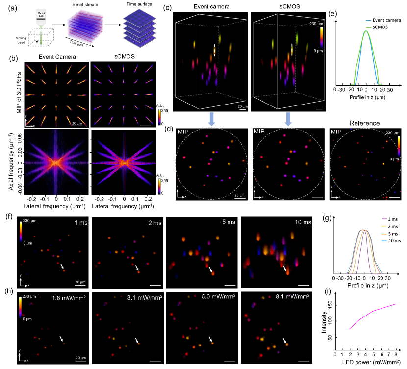
To validate the fidelity of the result of EventLFM, we conduct a comparative study with a standard Fourier LFM equipped with an sCMOS camera. First, we calibrate the 3D PSF for both systems. Given that the event camera can only capture dynamic objects, EventLFM PSFs are obtained from an event stream generated by a bead translating continuously through the system’s depth of field (DOF) at 0.2 mm/s, as illustrated in Fig. 2(a). For the standard Fourier LFM, PSFs are obtained by scanning a 1- $\mu$ m bead along the $z$ -axis. Subsequently, we analyze the lateral and axial resolutions by computing the 3D modulation transfer function (MTF) for both systems, defined by the 3D Fourier spectrum of the calibrated 3D PSF[8]. Figure 2(b) shows a strong agreement in both the 3D PSFs and the 3D MTFs between EventLFM and the standard Fourier LFM, thereby validating EventLFM’s ability to achieve high spatial resolution at a markedly improved frame rate (1000 Hz vs. 30 Hz). We note that the PSF measurements from the event camera are noisier than that from the sCMOS camera due to more pronounced noise from the measured event stream. Additional performance metrics of standard Fourier LFM, such as FOV, DOF and resolution, are elaborated in Section 1 of Supplement 1.

For an intuitive, side-by-side comparison, we simultaneously acquire data from a slowly moving 3D fluorescent beads phantom using both systems. Both datasets – comprising time-surface frames from EventLFM and sCMOS frames – are processed via the same light field refocusing algorithm to generate 3D reconstructions. Fig. 2(c) shows single-frame depth color-coded 3D reconstructions from both systems. The consistency between the two methods verifies EventLFM’s fidelity in reconstructing depth information throughout the DOF. To further confirm that EventLFM provides consistent axial resolution, intensity profiles extracted from the same bead along the white dashed lines are compared in Fig. 2(d). For further validation, conventional widefield fluorescence microscopy (Plan Apo, 20 $\times$ , 0.75 NA, Nikon) is also employed to capture a $z$ -stack of the same phantom (see details in Section 1 of Supplement 1). A comparison of depth color-coded maximum intensity projections (MIPs) across all three methods is shown in Fig. 2(e). The results confirm EventLFM’s capability for accurate volumetric reconstruction across the entire FOV. Intriguingly, we observe that the axial elongation achieved by EventLFM is slightly shorter than achieved by the standard Fourier LFM, as evidenced in both the 3D reconstructions (Fig. 2(d)) and axial profiles of individual beads (Fig. 2(e)). We attribute this observation to the unique event-driven signal acquisition mechanism of the event camera. Specifically, an accumulation time of 1 ms necessitates sufficient power to trigger events. When the illumination power is low, only the central region of the beads has adequate intensity to generate such events, which in turn reduces the axial elongation in the reconstructions.

We also characterize how EventLFM’s performance is affected by key experimental parameters, specifically the accumulation time of the event camera and the illumination power. The raw event stream from the event camera exhibits a temporal resolution of 1 $\mu$ s. When this data is transformed into frames, the user-defined accumulation time significantly influences the quality of the reconstruction. To demonstrate this, we image a fluorescent beads phantom moving at 2.5 mm/s along the $y$ direction. Similar to conventional cameras, an elongated accumulation time leads to increased averaged intensity and enlarged/blurred bead images, as shown in Fig. 2(f) and axial profiles in Fig. 2(g). By properly selecting an appropriate accumulation time based on sample’s brightness levels and event dynamics, the event camera can achieve superior resolution. It should be noted that this parameter is adjusted in the post-processing step without impacting the data capture speed. Next, while the event stream inherently lacks information on absolute intensity, we observe its sensitivity to variations in object brightness levels, as shown in Fig. 2(h). Intuitively, this is because a larger intensity variation produces more events in quick succession. To demonstrate this, we record the same fluorescent beads phantom moving at 1 mm/s along the $y$ direction under varying illumination powers, spanning 1.8 mW/mm² to 8.1 mW/mm², while keeping the accumulation time constant. The subsequent EventLFM reconstructions reveal a positive correlation between reconstructed intensity and illumination power, as depicted in Fig. 2(i).

3 Results

3.1 Imaging of fast-moving objects

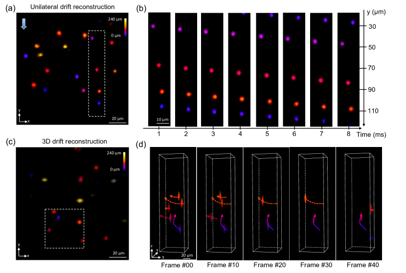
We substantiate the capability of EventLFM to reconstruct high-speed 3D motion, demonstrating its utility in capturing dynamical phenomena in biological contexts. First, we employ a motorized stage with a velocity range of 0.001 mm/s to 2.7 mm/s to execute controlled motion experiments. We image a 3D phantom comprising 2- $\mu$ m fluorescent beads moving at 2.5 mm/s. EventLFM successfully reconstructs the rapid movements across all depths at an effective frame rate of 1 kHz, as illustrated in Fig. 3(a). To better visualize the reconstructed 4D spatiotemporal information, we extract an ROI and present eight consecutive frames in Fig. 3(b). Given the object’s fixed velocity along the $x$ -axis, the bead positions calculated from the motorized stage setting align well with the EventLFM reconstructions. In contrast, the standard Fourier LFM using the sCMOS camera operating at 30 Hz suffers from severe motion blur artifacts. In addition, we also image the same object using the benchmark Fourier LFM system under static and slow-motion conditions (see details in Section 3 of Supplement 1). The results further corroborate the robustness of our EventLFM system. These controlled experiments confirm EventLFM’s efficacy in capturing rapid 3D dynamics at frame rates up to 1 kHz.

In the context of biological applications, the motion of many samples occurs over a gamut of velocities, directions, and depths. Acknowledging this complexity, we extend our EventLFM evaluations to scenarios involving uncontrolled complex 3D motion. Specifically, fluorescent beads are suspended in an alcohol-water droplet subjected to ultrasonic disintegration, inducing variable motion directions and velocities exceeding 2.5 mm/s. After performing EventLFM reconstructions, we present a depth color-coded MIP in Fig. 3(c). A selected sub-region, marked by a white dashed square, is subjected to volumetric rendering for 5 representative frames in Fig. 3(d). Leveraging the millisecond-level temporal resolution, we trace intricate trajectories (depicted as dotted lines with arrows) for individual beads. Notably, complex motion patterns – including depth fluctuations – are faithfully captured. For instance, a bead represented in blue in the frame labeled #00 in Fig. 3(d) exhibits helical movement through the volume over several microseconds. This affirms EventLFM’s utility in characterizing complex, high-speed 3D dynamics.

3.2 Imaging of dynamic blinking objects

In addition to capturing rapid motions, another important category of complex and dynamic biological processes entail rapidly blinking signals, such as those arising from neuronal activities. To evaluate EventLFM’s capability of tracking these types of dynamic signals, we employ a high-power LED driver (DC2200, Thorlabs) to generate adjustable pulsed illumination. In this proof-of-concept study, a 3D phantom embedded with fluorescent beads is illuminated using a variable pulse sequence, configured with a 1 ms pulse width and a variable pulse repetition rate ranging from 2 ms to 50 ms.

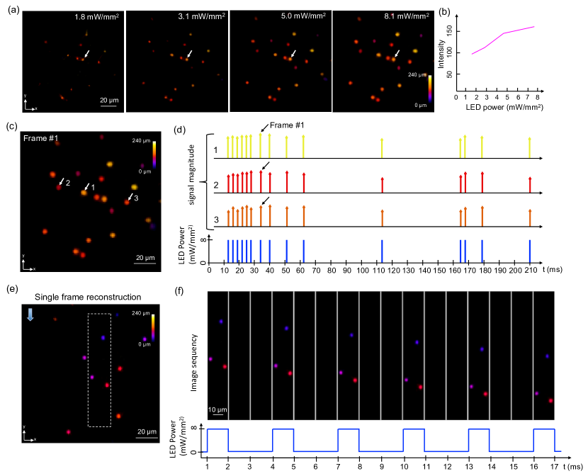
It should be noted that the event-based signal features from blinking objects differ from those of fast-moving objects. Thus, an additional system characterization tailored to blinking objects is carried out. In this experiment, we maintain a pulse width and accumulation time of 1 ms width, while the optical power when the LED is on is systematically altered between 1.8 mW/mm² and 8.1 mW/mm². As shown in Fig. 4(a), the reconstructed signal increases with the applied optical power. We further quantify this relationship by isolating a single bead and calculating its mean reconstructed intensity at various illumination powers; the resultant graph presented in Fig. 4(b) reveals an approximately linear relationship.

Next, we demonstrate EventLFM’s ability to image 3D objects blink at disparate intervals. For post-processing, a 1 ms accumulation time (equivalent to a 1 kHz frame rate) is set, synchronized to the onset of the first pulse. By employing the light field refocusing algorithm, we successfully reconstruct the blinking beads as displayed in Fig. 4(c). To further validate the system’s accuracy, three distinct beads (as marked in the MIP in Fig. 4(c)) are selected and their mean intensity signals calculated, as shown in Fig. 4(d). The temporal traces confirm that the reconstructed signals, despite slight fluctuations in intensities, are in agreement with the pre-configured LED pulse sequences. This result validates EventLFM’s capability in capturing high-frequency blinking signals in a 3D spatial context.

Lastly, to provide a comprehensive assessment, we introduce concurrent linear motion to the blinking objects by synchronizing pulsed illumination with translational movement of the 3D phantom via a motorized stage. A phantom embedded with fluorescent beads is used similar to earlier experiments. Parameters are also set similar to earlier experiments, with a pulse width of 1 ms and a 2 ms delay, while the object velocity is fixed at 2.5 mm/s. Figure 4(e) shows a depth color-coded MIP from a single reconstructed volume frame. To elucidate the dynamic objects further, Fig. 4(f) illustrates 16 consecutive frames within the white dashed rectangular region indicated in Fig. 4(e). These frames clearly show the expected linear motion and the blinking events are reconstructed at the expected timestamps. Each reconstructed bead is translated linearly along the $y$ -axis, as expected. Each signal-bearing frame is followed by two empty frames, which conform to the set LED pulse sequences shown in the bottom panel of Fig. 4(f). These results confirm EventLFM’s robust and reliable performance in capturing complex 3D dynamics.

3.3 Imaging of neuronal signals in scattering mouse brain tissue

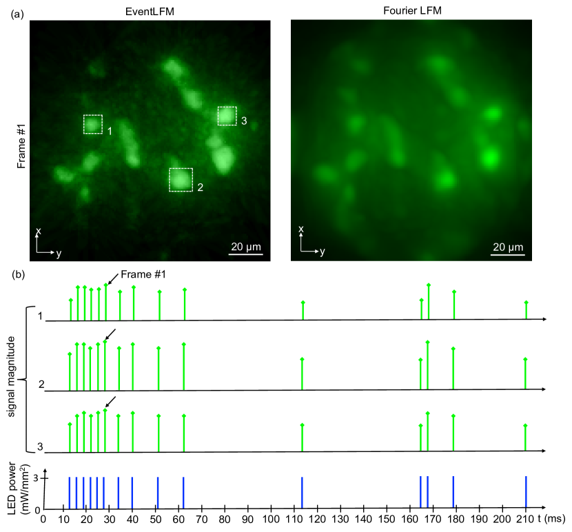
To demonstrate EventLFM’s potential for neural imaging, we image a 75 µm thick section of GFP-labeled mouse brain tissue. The sample is illuminated using a pulsed LED source, designed to simulate neuronal activities within scattering biological tissues. The illumination pulse sequence is set with a 1 ms pulse width and intervals varying from 2 ms to 50 ms. To validate the spatial reconstruction accuracy of EventLFM, we capture the fluorescence signals with traditional Fourier LFM and conventional fluorescent microscopy under constant illumination. Fig. 5(a) shows MIPs from a single reconstructed frame of each method. By visual inspection, the reconstruction from EventLFM is consistent with Fourier LFM, effectively capturing all neurons within the FOV and the intensity variations among them. However, a notable difference arises in the signal-to-background ratio (SBR). Fourier LFM suffers from a low SBR due to tissue scattering, which results in neuronal signals being buried in strong background fluorescence. In contrast, EventLFM demonstrates a significantly improved SBR, yielding a reconstruction with markedly improved image contrast and suppressed background fluorescence. This improvement is attributed to the event-based measurement mechanism intrinsic to EventLFM, wherein a readout is generated only when intensity changes exceed a certain threshold. Consequently, temporally slowly varying background fluorescence signals, which do not often meet this criterion, are either removed or substantially reduced in the raw data. Additionally, to underline EventLFM’s capability of precisely recording fast neuronal spikes, temporal traces from three distinct neurons are extracted, as shown in Fig. 5(b). These traces exhibit a strong correlation with the input illumination pulse sequence, thereby validating that EventLFM can accurately reconstruct neuronal blinking dynamics within scattering tissue.

3.4 Imaging of neuron-labeled freely-moving C. elegans

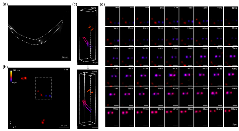
To further showcase EventLFM’s ability to capture complex biological dynamics, we employ it to track GFP-labeled neurons in a sample containing multiple C. elegans[37]. For the experiment, the C. elegans are positioned on a gel substrate and subsequently submerged in a droplet of S-Basal solution, thereby creating a 3D environment for their free movement. First, we identify four distinct GFP-expressing neurons using conventional fluorescent microscopy – two located in the tail region and another two in the mid-body section, as visualized in Fig. 6(a). Despite the relative sparsity of neurons, multiple C. elegans specimens are placed within the FOV. To accumulate enough event data for weaker neuronal signals, we set the accumulation time at 2 ms, yielding an effective frame rate of 500 Hz, which is sufficient for real-time 3D tracking of the organism. Using our EventLFM reconstruction algorithm, we generate depth color-coded MIP of the reconstructed volume frame at time 0 ms in Fig. 6(b), which clearly shows the spatial distribution of neurons across different depths for four distinct C. elegans. To further extract the neuronal dynamics, we focus on a specific region marked by a white dashed rectangle in Fig.6(b). Two temporally-separated 3D reconstructions from this region are presented at timestamps 42 ms and 92 ms in Fig. 6(c), complete with tracked trajectories marked in dashed lines. To further examine the neuronal movements, we present a time-series montage of the aforementioned area in Fig. 6(d) (additional results and comparisons with standard Fourier LFM are shown in Section 4 of Supplement 1). Notably, the neurons displayed in blue exhibit rapid and ascending motion across multiple axial planes over the time course. These result showcase EventLFM’s capability to accurately capture biological dynamics in a 3D space at ultra-high frame rates.

4 Conclusion

We present the first, to the best of our knowledge, ultrafast Fourier LFM system, EventLFM, that leverages an event camera and a tailored reconstruction algorithm to facilitate volumetric imaging at kHz speeds. By comparing the PSF, MTF and 3D reconstructions, we have established that EventLFM achieves a lateral resolution comparable to that of traditional Fourier LFM system. Notably, EventLFM provides marginally superior axial resolution and substantially improved temporal resolution. Our experimental results further underscore EventLFM’s versatility and capability. We demonstrate its effectiveness to reconstruct complex dynamics of rapidly moving 3D objects at 1 kHz temporal resolution. Moreover, through controlled illumination experiments, we showcase imaging of high-frequency 3D blinking objects with pulse widths as short as 1 ms. Additionally, we demonstrate EventLFM’s ability to capture rapid dynamic signals within scattering tissues by imaging neurons in a mouse brain section under a controlled LED pulse sequence designed to induce blinking signals at kHz rates. Lastly, we present imaging and tracking of GFP-expressing neurons in freely moving C. elegans within a 3D space, achieving a frame rate of 500 Hz.

Leveraging the unique properties of an event camera, EventLFM delivers kHz imaging capabilities with intrinsically lower data bandwidth requirements. The data stream is comprised of sparse 4D vectors, corresponding only to pixels that register an event within the acquisition window. Our current approach employs a time-surface method for event data processing, combined with median filtering to reduce sensor noise. However, the effectiveness of median filtering is limited, impacting the quality of the final reconstructions. For future developments, there are significant potentials for employing deep learning methods to address these limitations. For example, a deep neural network can be trained as an adaptive encoder to enhance the extraction of physically meaningful information from sparse event data while concurrently suppressing stochastic sensor noise [38, 39]. Broadly speaking, this paves the way for future research in developing advanced computational algorithms to fully exploit the sparsity of event data [40] in order to reconstruct more complex 3D processes over large volumes.

EventLFM significantly mitigates the low SBR challenges typically encountered in scattering environments [41] - a major limitation of traditional widefield microscopy techniques - as demonstrated by our experiment on mouse brain tissues. However, the light field refocusing algorithm used in this study, while straightforward, is susceptible to ghost artifacts and axial elongations in 3D reconstructions. Future work may develop more sophisticated reconstruction algorithms to minimize these artifacts, drawing on recent advances in computational imaging [8, 9]. This will lead to 3D reconstructions with improved quality and resolution. In addition, our work opens up tremendous opportunities for future research in event-driven imaging within scattering media [42] and the development of advanced computational algorithms that more effectively leverage event-driven measurement for extracting dynamic signals from deep within scattering tissues.

In conclusion, given its simplicity, ultrafast 3D imaging capability, and robustness in scattering environments, EventLFM has the potential to be a valuable tool in various biomedical applications for visualizing complex, dynamic 3D biological phenomena.

\bmsection

Funding This project has been made possible in part by National Institutes of Health (R01NS126596) and a grant from 5022 - Chan Zuckerberg Initiative DAF, an advised fund of Silicon Valley Community Foundation.

\bmsection

Acknowledgments The authors acknowledge Danchen Jia and Dr. Ji-Xin Cheng for generously lending us the microlens array, as well as Boston University Shared Computing Cluster for proving the computational resources.

\bmsection

Disclosures The authors declare no conflicts of interest.

\bmsection

Data Availability Data underlying the results presented in this paper may be obtained from the authors upon reasonable request.

\bmsection

Supplemental document See Supplement 1 for supporting content.

References

[1] J. Mertz, “Strategies for volumetric imaging with a fluorescence microscope,” \JournalTitleOptica 6, 1261–1268 (2019).
[2] M. Minsky, “Memoir on inventing the confocal scanning microscope,” \JournalTitleScanning 10, 128–138 (1988).
[3] F. Helmchen and W. Denk, “Deep tissue two-photon microscopy,” \JournalTitleNature Methods 2, 932–940 (2005).
[4] A. H. Voie, D. Burns, and F. Spelman, “Orthogonal-plane fluorescence optical sectioning: Three-dimensional imaging of macroscopic biological specimens,” \JournalTitleJournal of microscopy 170, 229–236 (1993).
[5] M. Levoy, R. Ng, A. Adams, M. Footer, and M. Horowitz, “Light field microscopy,” in Acm Siggraph 2006 Papers, (2006), pp. 924–934.
[6] C. Guo, W. Liu, X. Hua, H. Li, and S. Jia, “Fourier light-field microscopy,” \JournalTitleOptics Express 27, 25573 (2019).
[7] A. Llavador, J. Sola-Pikabea, G. Saavedra, B. Javidi, and M. Martínez-Corral, “Resolution improvements in integral microscopy with fourier plane recording,” \JournalTitleOptics express 24, 20792–20798 (2016).
[8] Y. Xue, I. G. Davison, D. A. Boas, and L. Tian, “Single-shot 3d wide-field fluorescence imaging with a computational miniature mesoscope,” \JournalTitleScience Advances 6, eabb7508 (2020).
[9] Y. Xue, Q. Yang, G. Hu, K. Guo, and L. Tian, “Deep-learning-augmented computational miniature mesoscope,” \JournalTitleOptica 9, 1009–1021 (2022).
[10] F. L. Liu, G. Kuo, N. Antipa, K. Yanny, and L. Waller, “Fourier diffuserscope: single-shot 3d fourier light field microscopy with a diffuser,” \JournalTitleOptics Express 28, 28969–28986 (2020).
[11] J. K. Adams, V. Boominathan, B. W. Avants, D. G. Vercosa, F. Ye, R. G. Baraniuk, J. T. Robinson, and A. Veeraraghavan, “Single-frame 3d fluorescence microscopy with ultraminiature lensless flatscope,” \JournalTitleScience advances 3, e1701548 (2017).
[12] S. Nelson and R. Menon, “Bijective-constrained cycle-consistent deep learning for optics-free imaging and classification,” \JournalTitleOptica 9, 26–31 (2022).
[13] E. Nehme, D. Freedman, R. Gordon, B. Ferdman, L. E. Weiss, O. Alalouf, T. Naor, R. Orange, T. Michaeli, and Y. Shechtman, “Deepstorm3d: dense 3d localization microscopy and psf design by deep learning,” \JournalTitleNature methods 17, 734–740 (2020).
[14] S. R. P. Pavani, M. A. Thompson, J. S. Biteen, S. J. Lord, N. Liu, R. J. Twieg, R. Piestun, and W. E. Moerner, “Three-dimensional, single-molecule fluorescence imaging beyond the diffraction limit by using a double-helix point spread function,” \JournalTitleProceedings of the National Academy of Sciences 106, 2995–2999 (2009).
[15] A. S. Abdelfattah, J. Zheng, A. Singh, Y.-C. Huang, D. Reep, G. Tsegaye, A. Tsang, B. J. Arthur, M. Rehorova, C. V. L. Olson, Y. Shuai, L. Zhang, T.-M. Fu, D. E. Milkie, M. V. Moya, T. D. Weber, A. L. Lemire, C. A. Baker, N. Falco, Q. Zheng, J. B. Grimm, M. C. Yip, D. Walpita, M. Chase, L. Campagnola, G. J. Murphy, A. M. Wong, C. R. Forest, J. Mertz, M. N. Economo, G. C. Turner, M. Koyama, B.-J. Lin, E. Betzig, O. Novak, L. D. Lavis, K. Svoboda, W. Korff, T.-W. Chen, E. R. Schreiter, J. P. Hasseman, and I. Kolb, “Sensitivity optimization of a rhodopsin-based fluorescent voltage indicator,” \JournalTitleNeuron 111, 1547–1563.e9 (2023).
[16] M. B. Bouchard, B. R. Chen, S. A. Burgess, and E. M. Hillman, “Ultra-fast multispectral optical imaging of cortical oxygenation, blood flow, and intracellular calcium dynamics,” \JournalTitleOptics express 17, 15670–15678 (2009).
[17] L. C. Rome and S. L. Lindstedt, “The quest for speed: muscles built for high-frequency contractions,” \JournalTitlePhysiology 13, 261–268 (1998).
[18] L. Gao, J. Liang, C. Li, and L. V. Wang, “Single-shot compressed ultrafast photography at one hundred billion frames per second,” \JournalTitleNature 516, 74–77 (2014).
[19] J. Liang and L. V. Wang, “Single-shot ultrafast optical imaging,” \JournalTitleOptica 5, 1113–1127 (2018).
[20] X. Liu, A. Skripka, Y. Lai, C. Jiang, J. Liu, F. Vetrone, and J. Liang, “Fast wide-field upconversion luminescence lifetime thermometry enabled by single-shot compressed ultrahigh-speed imaging,” \JournalTitleNature communications 12, 6401 (2021).
[21] Y. Ma, Y. Lee, C. Best-Popescu, and L. Gao, “High-speed compressed-sensing fluorescence lifetime imaging microscopy of live cells,” \JournalTitleProceedings of the National Academy of Sciences 118, e2004176118 (2021).
[22] X. Feng and L. Gao, “Ultrafast light field tomography for snapshot transient and non-line-of-sight imaging,” \JournalTitleNature Communications 12, 2179 (2021).
[23] T. D. Weber, M. V. Moya, K. Kılıç, J. Mertz, and M. N. Economo, “High-speed multiplane confocal microscopy for voltage imaging in densely labeled neuronal populations,” \JournalTitleNature Neuroscience pp. 1–9 (2023).
[24] J. Wu, Y. Liang, S. Chen, C.-L. Hsu, M. Chavarha, S. W. Evans, D. Shi, M. Z. Lin, K. K. Tsia, and N. Ji, “Kilohertz two-photon fluorescence microscopy imaging of neural activity in vivo,” \JournalTitleNature Methods 17, 287–290 (2020).
[25] J. Platisa, X. Ye, A. M. Ahrens, C. Liu, I. A. Chen, I. G. Davison, L. Tian, V. A. Pieribone, and J. L. Chen, “High-speed low-light in vivo two-photon voltage imaging of large neuronal populations,” \JournalTitleNature Methods 20, 1095–1103 (2023).
[26] S. Xiao, J. T. Giblin, D. A. Boas, and J. Mertz, “High-throughput deep tissue two-photon microscopy at kilohertz frame rates,” \JournalTitleOptica 10, 763–769 (2023).
[27] G. Gallego, T. Delbrück, G. Orchard, C. Bartolozzi, B. Taba, A. Censi, S. Leutenegger, A. J. Davison, J. Conradt, K. Daniilidis, and D. Scaramuzza, “Event-based vision: A survey,” \JournalTitleIEEE Transactions on Pattern Analysis and Machine Intelligence 44, 154–180 (2022).
[28] P. Lichtsteiner, C. Posch, and T. Delbruck, “A 128× 128 120 dB 15 $\mu$ s latency asynchronous temporal contrast vision sensor,” \JournalTitleIEEE Journal of Solid State Circuits 43, 566–576 (2008).
[29] C. E. Willert, “Event-based imaging velocimetry using pulsed illumination,” \JournalTitleExperiments in Fluids 64, 98 (2023).
[30] G. Chen, H. Cao, J. Conradt, H. Tang, F. Rohrbein, and A. Knoll, “Event-based neuromorphic vision for autonomous driving: A paradigm shift for bio-inspired visual sensing and perception,” \JournalTitleIEEE Signal Processing Magazine 37, 34–49 (2020).
[31] A. Amir, B. Taba, D. Berg, T. Melano, J. McKinstry, C. Di Nolfo, T. Nayak, A. Andreopoulos, G. Garreau, M. Mendoza et al., “A low power, fully event-based gesture recognition system,” in Proceedings of the IEEE conference on computer vision and pattern recognition, (2017), pp. 7243–7252.
[32] C. Cabriel, T. Monfort, C. G. Specht, and I. Izeddin, “Event-based vision sensor for fast and dense single-molecule localization microscopy,” \JournalTitleNature Photonics (2023).
[33] R. Mangalwedhekar, N. Singh, C. S. Thakur, C. S. Seelamantula, M. Jose, and D. Nair, “Achieving nanoscale precision using neuromorphic localization microscopy,” \JournalTitleNature Nanotechnology 18, 380–389 (2023).
[34] X. Lagorce, G. Orchard, F. Galluppi, B. E. Shi, and R. B. Benosman, “HOTS: A hierarchy of event-based time-surfaces for pattern recognition,” \JournalTitleIEEE Transactions on Pattern Analysis and Machine Intelligence 39, 1346–1359 (2017).
[35] A. Sironi, M. Brambilla, N. Bourdis, X. Lagorce, and R. Benosman, “Hats: Histograms of averaged time surfaces for robust event-based object classification,” in Proceedings of the IEEE Conference on Computer Vision and Pattern Recognition (CVPR), (2018).
[36] R. Ng, M. Levoy, M. Brédif, G. Duval, M. Horowitz, and P. Hanrahan, “Light field photography with a hand-held plenoptic camera,” Ph.D. thesis, Stanford University (2005).
[37] G. Wang, L. Sun, C. P. Reina, I. Song, C. V. Gabel, and M. Driscoll, “Ced-4 card domain residues can modulate non-apoptotic neuronal regeneration functions independently from apoptosis,” \JournalTitleScientific Reports 9, 13315 (2019).
[38] Z. Zhang, J. Suo, and Q. Dai, “Denoising of event-based sensors with deep neural networks,” in Optoelectronic Imaging and Multimedia Technology VIII, vol. 11897 (SPIE, 2021), pp. 203–209.
[39] J. Hagenaars, F. Paredes-Vallés, and G. De Croon, “Self-supervised learning of event-based optical flow with spiking neural networks,” \JournalTitleAdvances in Neural Information Processing Systems 34, 7167–7179 (2021).
[40] J. K. Eshraghian, M. Ward, E. O. Neftci, X. Wang, G. Lenz, G. Dwivedi, M. Bennamoun, D. S. Jeong, and W. D. Lu, “Training spiking neural networks using lessons from deep learning,” \JournalTitleProceedings of the IEEE 111, 1016–1054 (2023).
[41] J. Alido, J. Greene, Y. Xue, G. Hu, Y. Li, K. J. Monk, B. T. DeBenedicts, I. G. Davison, and L. Tian, “Robust single-shot 3d fluorescence imaging in scattering media with a simulator-trained neural network,” \JournalTitlearXiv preprint arXiv:2303.12573 (2023).
[42] N. Zhang, T. Shea, and A. Nurmikko, “Event-driven imaging in turbid media: A confluence of optoelectronics and neuromorphic computation,” \JournalTitlearXiv preprint arXiv:2309.06652 (2023).

See pages 1,2,3,4,5,6,7 of EventLFM_SI