Subtractive Mixture Models via Squaring:
Representation and Learning

Abstract

Mixture models are traditionally represented and learned by adding several distributions as components. Allowing mixtures to subtract probability mass or density can drastically reduce the number of components needed to model complex distributions. However, learning such subtractive mixtures while ensuring they still encode a non-negative function is challenging. We investigate how to learn and perform inference on deep subtractive mixtures by squaring them. We do this in the framework of probabilistic circuits, which enable us to represent tensorized mixtures and generalize several other subtractive models. We theoretically prove that the class of squared circuits allowing subtractions can be exponentially more expressive than traditional additive mixtures; and, we empirically show this increased expressiveness on a series of real-world distribution estimation tasks.

1 Introduction

Finite mixture models (MMs) are a staple in probabilistic machine learning, as they offer a simple and elegant solution to model complex distributions by blending simpler ones in a linear combination (McLachlan et al., 2019). The classical recipe to design MMs is to compute a convex combination over input components. That is, a MM representing a probability distribution $p$ over a set of random variables $\bm{\mathrm{X}}=\{X_{1},X_{2},\ldots,X_{D}\}$ is usually defined as

$$\textstyle p(\bm{\mathrm{X}})=\sum\nolimits_{i=1}^{K}w_{i}p_{i}(\bm{\mathrm{X}}),\quad\text{with}\quad w_{i}\geq 0,\quad\sum\nolimits_{i=1}^{K}w_{i}=1,$$ (1)

where $w_{i}$ are the mixture parameters and each component $p_{i}$ is a mass or density function. This is the case for widely-used MMs such as Gaussian mixture models (GMMs) and hidden Markov models (HMMs) but also mixtures of generative models such as normalizing flows (Papamakarios et al., 2021) and deep mixture models such as probabilistic circuits (PCs, Vergari et al., 2019b).

The convexity constraint in Eq. 1 is the simplest sufficient condition to ensure that $p$ is a non-negative function and integrates to 1, i.e., is a valid probability distribution, and is often assumed in practice. However, this implies that the components $p_{i}$ can only be combined in an additive manner and as such it can greatly impact their ability to estimate a distribution efficiently. For instance, consider approximating distributions having “holes” in their domain, such as the simple 2-dimensional ring distribution on the left (ground truth). A classical additive MM such a GMM would ultimately recover it, as it is a universal approximator of density functions (Nguyen et al., 2019), but only by employing an unnecessarily high number of components. A MM allowing negative mixture weights, i.e., $w_{i}<0$, would instead require only two components, as it can subtract one outer Gaussian density from an inner one (NGMM). We call these MMs subtractive or non-monotonic MMs (NMMs), as opposed to their classical additive counterpart, called monotonic MMs (Shpilka & Yehudayoff, 2010).

The challenge with NMMs is ensuring that the modeled $p(\bm{\mathrm{X}})$ is a valid distribution, as the convexity constraint does not hold anymore. This problem has been investigated in the past in a number of ways, in its simplest form by imposing ad-hoc constraints over the mixture parameters $w_{i}$, derived for simple components such as Gaussian and Weibull distributions (Zhang & Zhang, 2005; Rabusseau & Denis, 2014; Jiang et al., 1999). However, different families of components would require formulating different constraints, whose closed-form existence is not guaranteed.

In this paper, we study a more general principle to design NMMs that circumvents the aforementioned limitation while ensuring non-negativity of the modeled function: squaring the encoded linear combination. For example, the NGMM above is a squared combination of Gaussian densities with negative mixture parameters. We theoretically investigate the expressive efficiency of squared NMMs, i.e., their expressiveness w.r.t. their model size, and show how to effectively represent and learn them in practice. Specifically, we do so in the framework of PCs, tractable models generalizing classical shallow MMs into deep MMs represented as structured neural networks. Deep PCs are already more expressive efficient than shallow MMs as they compactly encode a mixture with an exponential number of components (Vergari et al., 2019b; Choi et al., 2020). However, they are classically represented with non-negative parameters, hence being restricted to encode deep but additive MMs. Instead, as a main theoretical contribution we prove that our squared non-monotonic PCs (NPC²s) can be exponentially more parameter-efficient than their monotonic counterparts.

Contributions. i) We introduce a general framework to represent NMMs via squaring (Sec. 2), within the language of tensorized PCs (Mari et al., 2023), and show how NPC²s can be effectively learned and used for tractable inference (Sec. 3). ii) We show how NPC²s generalize not only monotonic PCs but other apparently different models allowing negative parameters that have emerged in different literatures, such as square root of density models in signal processing (Pinheiro & Vidakovic, 1997), positive semi-definite (PSD) models in kernel methods (Rudi & Ciliberto, 2021), and Born machines from quantum mechanics (Orús, 2013) (Sec. 4). This allows us to understand why they lead to tractable inference via the property-oriented framework of PCs. iii) We derive an exponential lower bound over the size of monotonic PCs to represent functions that can be compactly encoded by one NPC² (Sec. 4.1), hence showing that NPC²s (and thus the aforementioned models) can be more expressive for a given size. Finally, iv) we provide empirical evidence (Sec. 5) that NPC²s can approximate distributions better than monotonic PCs for a variety of experimental settings involving learning from real-world data and distilling intractable models such as large language models to unlock tractable inference (Zhang et al., 2023).

2 Subtractive Mixtures via Squaring

We start by formalizing how to represent shallow NMMs by squaring non-convex combinations of $K$ simple functions. Like exponentiation in energy-based models (LeCun et al., 2006), squaring ensures the non-negativity of our models, but differently from it, allows to tractably renormalize them. A squared NMM encodes a (possibly unnormalized) distribution $c^{2}(\bm{\mathrm{X}})$ over variables $\bm{\mathrm{X}}$ as

$$\textstyle c^{2}(\bm{\mathrm{X}})=\left(\sum\nolimits_{i=1}^{K}w_{i}c_{i}(\bm{\mathrm{X}})\right)^{2}=\sum\nolimits_{i=1}^{K}\sum\nolimits_{j=1}^{K}w_{i}w_{j}c_{i}(\bm{\mathrm{X}})c_{j}(\bm{\mathrm{X}}),$$ (2)

where $c_{i}$ are the learnable components and the mixture parameters $w_{i}\in\mathbb{R}$ are unconstrained, as opposed to Eq. 1. Squared NMMs can therefore represent $\binom{K+1}{2}$ components within the same parameter budget of $K$ components of an additive MM. Each component of a squared NMM computes a product of experts $c_{i}(\bm{\mathrm{X}})c_{j}(\bm{\mathrm{X}})$ (Hinton, 2002) allowing negative parameters $2w_{i}w_{j}$ if $i\neq j$, and $c_{i}^{2}(\bm{\mathrm{X}})$ with $w_{i}^{2}$ otherwise. Fig. 1 shows a concrete example of this construction, which constitutes the simplest NPC² we can build (see Sec. 3), i.e., comprising a single layer and having depth one.

Tractable marginalization. Analogously to traditional MMs, squared NMMs support tractable marginalization and conditioning, if their component distributions do as well. The distribution encoded by $c^{2}(\bm{\mathrm{X}})$ can be normalized to compute a valid probability distribution $p(\bm{\mathrm{X}})=c^{2}(\bm{\mathrm{X}})/Z$, by computing its partition function $Z$ as

$$\textstyle Z=\int c^{2}(\bm{\mathrm{x}})\,\mathrm{d}\bm{\mathrm{x}}=\sum\nolimits_{i=1}^{K}\sum\nolimits_{j=1}^{K}w_{i}w_{j}\int c_{i}(\bm{\mathrm{x}})c_{j}(\bm{\mathrm{x}})\,\mathrm{d}\bm{\mathrm{x}}.$$ (3)

Computing $Z$ translates to evaluating $\binom{K+1}{2}$ integrals over products of components $c_{i}(\bm{\mathrm{X}})c_{j}(\bm{\mathrm{X}})$. More generally, marginalizing any subset of variables in $\bm{\mathrm{X}}$ can be done in $\mathcal{O}(K^{2})$. This however implies that the components $c_{i}$ are chosen from a family of functions such that their product $c_{i}(\bm{\mathrm{X}})c_{j}(\bm{\mathrm{X}})$ can be tractably integrated, and $Z$ is non-zero and finite. This is true for many parametric families, including exponential families (Seeger, 2005). For instance, the product of two Gaussian or two categorical distributions is another Gaussian (Rasmussen & Williams, 2005) or categorical up to a multiplicative factor, which can be computed in polynomial time.

A wider choice of components. Note that we do not require each $c_{i}$ to model a probability distribution, e.g., we might have $c_{i}(\bm{\mathrm{x}})<0$. This allows us to employ more expressive tractable functions as base components in squared NMMs such as splines (see App. E for details) or potentially small neural networks (see discussion in Sec. 4.2). However, if the components are already flexible enough there might not be an increase in expressiveness when mixing them in a linear combination or squaring them. E.g., a simple categorical distribution can already capture any discrete distribution with finite support and a (subtractive) mixture thereof might not yield additional benefits besides being easier to learn. An additive mixture of Binomials is instead more expressive than a single Binomial, but expected to be less expressive than its subtractive version (as illustrated in Sec. 5).

Learning squared NMMs. The canonical way to learn traditional MMs (Eq. 1) is by maximum-likelihood estimation (MLE), i.e., by maximizing $\sum_{\bm{\mathrm{x}}\in\mathcal{D}}\log p(\bm{\mathrm{x}})$ where $\mathcal{D}$ is a set of independent and identically distributed (i.i.d.) samples. For squared NMMs, the MLE objective is

$$\textstyle\sum\nolimits_{\bm{\mathrm{x}}\in\mathcal{D}}\log\left(c^{2}(\bm{\mathrm{x}})/Z\right)=-|\mathcal{D}|\log Z+2\sum\nolimits_{\bm{\mathrm{x}}\in\mathcal{D}}\log|c(\bm{\mathrm{x}})|,$$ (4)

where $c(\bm{\mathrm{x}})=\sum_{i=1}^{K}w_{i}c_{i}(\bm{\mathrm{x}})$. Unlike other NMMs mentioned in Sec. 1, we do not need to derive additional closed-form constraints for the parameters to preserve non-negativity. Although materializing the squared mixture having $\binom{K+1}{2}$ components is required to compute $Z$ as in Eq. 3, evaluating $\log|c(\bm{\mathrm{x}})|$ is linear in $K$. Hence, we can efficiently perform batched stochastic gradient-based optimization and compute $Z$ just once per batch.

Figure 1: Shallow MMs and squared NMMs represented as PCs, mapped to a computational graph having input components and a weighted sum unit as output. Squaring a mixture with $K=3$ components (left) can yield more components that share parameters (right).

3 Squaring Deep Mixture Models

So far, we dealt with mixtures that are shallow, i.e., that can be represented as simple computational graphs with a single weighted sum unit (e.g., Fig. 1). We now generalize them in the framework of PCs (Vergari et al., 2019b; Choi et al., 2020; Darwiche, 2001) as they offer a property-driven language to model structured neural networks which allow tractable inference. PCs enable us to encode an exponential number of mixture components in a compact but deep computational graph.

PCs are usually defined in terms of scalar computational units: sum, product and input (App. A). Following Vergari et al. (2019a); Mari et al. (2023), we instead formalize them as tensorized computational graphs. That is, we group several computational units together in layers, whose advantage is twofold. First, we are able to derive a simplified tractable algorithm for squaring that requires only linear algebra operations and benefits from GPU acceleration (Alg. 1). Second, we can more easily generalize many recent PC architectures (Peharz et al., 2020b; a; Liu & Van den Broeck, 2021), as well as other tractable tensor representations (Sec. 4). We start by defining deep computational graphs that can model possibly negative functions, simply named circuits (Vergari et al., 2021).

Definition 1 (Tensorized circuit).

A tensorized circuit $c$ is a parametrized computational graph encoding a function $c(\bm{\mathrm{X}})$ and comprising of three kinds of layers: input, product and sum. Each layer comprises computational units defined over the same set of variables, also called its scope, and every non-input layer receives input from one or more layers. The scope of each non-input layer is the union of the scope of its inputs, and the scope of the output layer computing $c(\bm{\mathrm{X}})$ is $\bm{\mathrm{X}}$. Each input layer $\bm{\mathrm{\ell}}$ has scope $\bm{\mathrm{Y}}\subseteq\bm{\mathrm{X}}$ and computes a collection of $K$ functions $f_{i}(\bm{\mathrm{Y}})\in\mathbb{R}$, i.e., $\bm{\mathrm{\ell}}$ outputs a $K$-dimensional vector. Each product layer $\bm{\mathrm{\ell}}$ computes an Hadamard (or element-wise) product over the $N$ layers it receives as input, i.e., $\bm{\mathrm{\ell}}=\odot_{i=1}^{N}\bm{\mathrm{\ell}}_{i}$. A sum layer with $S$ sum units and receiving input form a previous layer $\bm{\mathrm{\ell}}\in\mathbb{R}^{K}$, is parametrized by $\bm{\mathrm{W}}\in\mathbb{R}^{S\times K}$ and computes $\bm{\mathrm{W}}\bm{\mathrm{\ell}}$.

Fig. 2 shows a deep circuit in tensorized form. To model a distribution via circuits we first require that the output of the computational graph is non-negative. We call such a circuit a PC. Similarly to shallow additive MM (Eq. 1), a sufficient condition to ensure non-negativity of the output is make the PC monotonic, i.e., to parameterize all sum layers with non-negative matrices and to restrict input layers to encode non-negative functions (e.g., probability mass or density functions). So far, monotonic PCs have been the canonical way to represent and learn PCs (Sec. 4.2). In Def. 1 we presented product layers computing Hadamard products only, to simplify notation and as this implementation choice is commonly used in many existing PC architectures (Darwiche, 2009; Liu & Van den Broeck, 2021; Mari et al., 2023). We generalize our treatment of PCs in Def. A.6 to deal with another popular product layer implementation: Kronecker products (Peharz et al., 2020b; a; Mari et al., 2023). Our results still hold for both kinds of product layers, if not specified otherwise.

Figure 2: Squaring tensorized structured-decomposable circuits reduces to squaring layers, depicted as colored boxes of ​ ​ (input), ​ ​ (product), and ​

a classic, real deep, Voltaire

​ (sum). Connections to a sum layer are labeled by the matrix parameterizing the layer, while connections to product layers are labeled by the Hadamard product sign (see also Fig. A.1). A tensorized structured-decomposable circuit (b) over three variables defined from the RG in (a) is squared in (c) by recursively squaring each layer via Alg. 1. Squared layers contain a quadratic number of units, but are still vectors.

Building tractable circuits for marginalization. Deep PCs can be renormalized and marginalize out any subset of $\bm{\mathrm{X}}$ in a single feed-forward pass if they are smooth and decomposable, i.e., each sum layer receives inputs from layers whose units are defined over the same scopes, and each product layer receives inputs from layers whose scopes are pairwise disjoint, respectively. See Prop. A.1 for more background. Sum layers in our Def. 1 guarantee smoothness by design as they have exactly one input. A simple way to ensure decomposability is to create a circuit that follows a hierarchical scope partitioning of variables $\bm{\mathrm{X}}$, also called a region graph.

Definition 2 (Region graph (Dennis & Ventura, 2012)).

Given a set of variables $\bm{\mathrm{X}}$, a region graph (RG) is a bipartite and rooted graph whose nodes are either regions, denoting subsets $\mathcal{R}$ of $\bm{\mathrm{X}}$, or partitions specifying how a region is partitioned into other regions.

Fig. 2 shows an example of a RG. Given a RG, we can build a smooth and decomposable tensorized circuit as follows. First, we parameterize regions that are not further partitioned $\mathcal{R}\subseteq\bm{\mathrm{X}}$ with an input layer encoding some functions over variables in $\mathcal{R}$. Then, we parameterize each partitioning $\{\mathcal{R}_{i}\}_{i=1}^{N}$ with a product layer having as inputs one layer for each $\mathcal{R}_{i}$. Each product layer is then followed by a sum layer. Figs. 2 and 2 illustrates such a construction by color-coding regions and corresponding layers. This will also provide us a clean recipe to efficiently square a deep circuit.

(Squared negative) MMs as circuits. It is easy to see that traditional shallow MMs (Eq. 1) can be readily represented as tensorized smooth and decomposable PCs consisting of an input layer encoding $K$ components $p_{i}$ followed by a sum layer, which is parametrized by a non-negative row-vector $\bm{\mathrm{W}}\in\mathbb{R}_{+}^{1\times K}$ whose entries sum up to one. Squared NMMs (Eq. 2) can be represented in a similar way, as they can be viewed as mixtures over an increased number of components (see Fig. 1 and Fig. A.1), where the sum layer is parameterized by real entries, instead. Next, we discuss how to square deep tensorized circuits as to retrieve our NPC²s model class.

Squaring (and renormalizing) tensorized circuits. The challenge of squaring a tensorized non-monotonic circuit $c$ (potentially encoding a negative function) is guaranteeing $c^{2}$ to be representable as a smooth and decomposable PC with polynomial size, as these two properties are necessary conditions to being able to renormalize $c^{2}$ efficiently and in a single feed-forward pass (Choi et al., 2020). In general, even squaring a decomposable circuit while preserving decomposability of the squared circuit is a #P-hard problem (Shen et al., 2016; Vergari et al., 2021). Fortunately, it is possible to obtain a decomposable representation of $c^{2}$ efficiently for circuits $c$ that are structured-decomposable (Pipatsrisawat & Darwiche, 2008; Vergari et al., 2021). Intuitively, in a tensorized structured-decomposable circuit all product layers having the same scope $\bm{\mathrm{Y}}\subseteq\bm{\mathrm{X}}$ decompose $\bm{\mathrm{Y}}$ over their input layers in the exact same way. We formalize this property in the Appendix in Def. A.3.

Tensorized circuits satisfying this property by design can be easily constructed by stacking layers conforming to a RG, as discussed before, and requiring that such a RG is a tree, i.e., in which there is a single way to partition each region, and whose input regions do not have overlapping scopes. E.g., the RG in Fig. 2 is a tree RG. From here on, w.l.o.g. we assume our tree RGs to be binary trees, i.e., they partition each region into two other regions only. Given a tensorized structured-decomposable circuit $c$ defined on such a tree RG, Alg. 1 efficiently constructs a smooth and decomposable tensorized circuit $c^{2}$. Moreover, let $L$ be the number of layers and $M$ the maximum time required to evaluate one layer in $c$, then the following proposition holds.

Proposition 1 (Tractable marginalization of squared circuits).

Let $c$ be a tensorized structured-decomposable circuit where the products of functions computed by each input layer can be tractably integrated. Any marginalization of $c^{2}$ obtained via Alg. 1 requires time and space $\mathcal{O}(L\cdot M^{2})$.

See Sec. B.2 for a proof. In a nutshell, this is possible because Alg. 1 recursively squares each layer $\bm{\mathrm{\ell}}$ in $c$ such as $\bm{\mathrm{\ell}}^{2}=\bm{\mathrm{\ell}}\otimes\bm{\mathrm{\ell}}$ in $c^{2}$, where $\otimes$ denotes the Kronecker product of two vectors. Our tensorized treatment of circuits allows for a much more compact version of the more general algorithm proposed in Vergari et al. (2021) which was defined in terms of squaring scalar computational units. At the same time, it lets us derive a tighter worst-case upper-bound than the one usually reported for squaring structured-decomposable circuits (Pipatsrisawat & Darwiche, 2008; Choi et al., 2015; Vergari et al., 2021), which is the squared number of computations in the whole computational graph, or $\mathcal{O}(L^{2}\cdot M^{2})$. Note that materializing $c^{2}$ is needed when we want to efficiently compute the normalization constant $Z$ of $c^{2}$ or marginalizing any subset of variables. As such, when learning by MLE (Eq. 4) and by batched gradient descent, we need to evaluate $c^{2}$ only once per batch, thus greatly amortizing its cost as we show in App. C. Finally, tractable marginalization enables tractable sampling from the distribution modeled by NPC²s, as we discuss in Sec. A.2.

Algorithm 1 $\textsf{squareTensorizedCircuit}(\bm{\mathrm{\ell}},\mathcal{R})$

Input: A tensorized circuit having output layer $\bm{\mathrm{\ell}}$ and defined on a tree RG rooted by $\mathcal{R}$.
Output: The tensorized squared circuit defined on the same tree RG having $\bm{\mathrm{\ell}}^{2}$ as output layer computing $\bm{\mathrm{\ell}}\otimes\bm{\mathrm{\ell}}$.

1:if $\bm{\mathrm{\ell}}$ is an input layer then

2:     $\bm{\mathrm{\ell}}$ computes $K$ functions $f_{i}(\mathcal{R})$

3:     return An input layer $\bm{\mathrm{\ell}}^{2}$ computing all $K^{2}$

4:          product combinations $f_{i}(\mathcal{R})f_{j}(\mathcal{R})$

5:else if $\bm{\mathrm{\ell}}$ is a product layer then

6:     $\{(\bm{\mathrm{\ell}}_{\textsf{i}},\mathcal{R}_{\textsf{i}}),\ (\bm{\mathrm{\ell}}_{\textsf{ii}},\mathcal{R}_{\textsf{ii}})\}\leftarrow\textsf{getInputs}(\bm{\mathrm{\ell}},\mathcal{R})$

7:     $\bm{\mathrm{\ell}}_{\textsf{i}}^{2}\leftarrow\textsf{squareTensorizedCircuit}(\bm{\mathrm{\ell}}_{\textsf{i}},\mathcal{R}_{\textsf{i}})$

8:     $\bm{\mathrm{\ell}}_{\textsf{ii}}^{2}\leftarrow\textsf{squareTensorizedCircuit}(\bm{\mathrm{\ell}}_{\textsf{ii}},\mathcal{R}_{\textsf{ii}})$

9:     return $\bm{\mathrm{\ell}}_{\textsf{i}}^{2}\odot\bm{\mathrm{\ell}}_{\textsf{ii}}^{2}$

10:else$\triangleright$ $\bm{\mathrm{\ell}}$ is a sum layer

11:     $\{(\bm{\mathrm{\ell}}_{\mathsf{i}},\mathcal{R})\}\leftarrow\textsf{getInputs}(\bm{\mathrm{\ell}},\mathcal{R})$

12:     $\bm{\mathrm{\ell}}_{\mathsf{i}}^{2}\leftarrow\textsf{squareTensorizedCircuit}(\bm{\mathrm{\ell}}_{\mathsf{i}},\mathcal{R})$

13:     $\bm{\mathrm{W}}\in\mathbb{R}^{S\times K}\leftarrow\textsf{getParameters}(\bm{\mathrm{\ell}})$

14:     $\bm{\mathrm{W}}^{\prime}\in\mathbb{R}^{S^{2}\times K^{2}}\leftarrow\bm{\mathrm{W}}\otimes\bm{\mathrm{W}}$

15:     return $\bm{\mathrm{W}}^{\prime}\bm{\mathrm{\ell}}_{\mathsf{i}}^{2}$

Numerical stability. Renormalizing deep PCs can easily lead to underflows and/or overflows. In monotonic PCs this is usually addressed by performing computations in log-space and utilizing the log-sum-exp trick (Blanchard et al., 2021). However, this is not applicable to non-monotonic PCs as intermediate layers can compute negative values. Therefore, we derive a signed log-sum-exp trick for which we represent the output of each layer $\bm{\mathrm{\ell}}\in\mathbb{R}^{S},\bm{\mathrm{\ell}}\neq\bm{0}$ in terms of their element-wise logarithm of absolute value $\log|\bm{\mathrm{\ell}}|$ and their element-wise sign $\operatorname{sign}(\bm{\mathrm{\ell}})\in\{-1,1\}^{S}$, and evaluate the circuit by propagating both. See App. D for details.

4 Expressiveness of NPC²s and Relationship to Other Models

Circuits have been used as the “lingua franca” to represent apparently different tractable model representations (Darwiche & Marquis, 2002; Shpilka & Yehudayoff, 2010), and to investigate their ability to exactly represent certain function families with only a polynomial increase in model size – also called the expressive efficiency (Martens & Medabalimi, 2014), or succinctness (de Colnet & Mengel, 2021) of a model class. This is because the size of circuits directly translates to the computational complexity of performing inference. As we extend the language of monotonic PCs to include negative parameters, here we provide polytime reductions from tractable probabilistic model classes emerging from different application fields that can encode subtractions, to (deep) non-monotonic PCs. By doing so, we not only shed a light on why they are tractable, by explicitly stating their structural properties as circuits, but also on why they can be more expressive than classical additive MMs, as we prove that NPC²s can be exponentially more compact in Sec. 4.1.

Simple shallow NMMs have been investigated for a limited set of component families, as discussed in Sec. 1. Notably, this can also be done by directly learning to approximate the square root of a density function, as done in signal processing with wavelet functions as components (Daubechies, 1992; Pinheiro & Vidakovic, 1997) or RBF kernels, i.e., unnormalized Gaussians centered over data points (Schölkopf & Smola, 2001), as in Hong & Gao (2021). As discussed in Sec. 3, we can readily represent these NMMs as simple NPC²s where kernel functions are computed by input layers.

Positive semi-definite (PSD) models (Rudi & Ciliberto, 2021; Marteau-Ferey et al., 2020) are a recent class of models from the kernel and optimization literature. Given a kernel function $\kappa$ (e.g., an RBF kernel as in Rudi & Ciliberto (2021)) and a set of $d$ data points $\bm{\mathrm{x}}^{(1)},\ldots,\bm{\mathrm{x}}^{(d)}$ with $\bm{\mathrm{\kappa}}(\bm{\mathrm{x}})=[\kappa(\bm{\mathrm{x}},\bm{\mathrm{x}}^{(1)}),\ldots,\kappa(\bm{\mathrm{x}},\bm{\mathrm{x}}^{(d)})]^{\top}\in\mathbb{R}^{d}$, and a real $d\times d$ PSD matrix $\bm{\mathrm{A}}$, they define an unnormalized distribution as the non-negative function $f(\bm{\mathrm{x}};\bm{\mathrm{A}},\bm{\mathrm{\kappa}})=\bm{\mathrm{\kappa}}(\bm{\mathrm{x}})^{\top}\bm{\mathrm{A}}\bm{\mathrm{\kappa}}(\bm{\mathrm{x}})$. Although apparently different, they they can be translated to NPC²s in polynomial time.

Proposition 2 (Reduction from PSD models).

A PSD model with kernel function $\kappa$, defined over $d$ data points, and parameterized by a PSD matrix $\bm{\mathrm{A}}$, can be represented as a mixture of squared NMMs (hence NPC²s) in time $\mathcal{O}(d^{3})$.

We prove this in Sec. B.3. Note that while PSD models are shallow non-monotonic PCs, we can stack them into deeper NPC²s that support tractable marginalization via structured-decomposability.

Tensor networks and the Born rule. Squaring a possibly negative function to retrieve an unnormalized distribution is related to the Born rule in quantum mechanics (Dirac, 1930), used to characterize the distribution of particles by squaring their wave function (Schollwoeck, 2010; Orús, 2013). These functions can be represented as a large $D$-dimensional tensor $\mathcal{T}$ over discrete variables $\bm{\mathrm{X}}=\{X_{1},\ldots,X_{D}\}$ taking value $\{1,\ldots,m\}$, compactly factorized in a tensor network (TN) such as a matrix-product state (MPS) (Pérez-García et al., 2007), also called tensor-train. Given an assignment $\bm{\mathrm{x}}=\langle x_{1},\ldots,x_{D}\rangle$ to $\bm{\mathrm{X}}$, a rank $r$ MPS compactly represents $\mathcal{T}$ as

$$\mathcal{T}[x_{1},\ldots,x_{D}]=\sum_{i_{1}=1}^{r}\sum_{i_{2}=1}^{r}\cdots\sum_{i_{D-1}=1}^{r}\bm{\mathrm{A}}_{1}[x_{1},i_{1}]\bm{\mathrm{A}}_{2}[x_{2},i_{1},i_{2}]\cdots\bm{\mathrm{A}}_{D}[x_{D},i_{D-1}]$$ (5)

where $\bm{\mathrm{A}}_{1},\bm{\mathrm{A}}_{D}\in\mathbb{R}^{m\times r}$, $\bm{\mathrm{A}}_{j}\in\mathbb{R}^{m\times r\times r}$ with $1<j<D$, for indices $\{i_{1},\ldots,i_{D-1}\}$, and denoting indexing with square brackets. To encode a distribution $p(\bm{\mathrm{X}})$, one can reparameterize tensors $\bm{\mathrm{A}}_{j}$ to be non-negative (Novikov et al., 2021) or apply the Born rule and square $\mathcal{T}$ to model $p(\bm{\mathrm{x}})\propto(\mathcal{T}[x_{1},\ldots,x_{D}])^{2}$. Such a TN is called a Born machine (BM) (Glasser et al., 2019). Besides modeling complex quantum states, TNs such as BMs have also been explored as classical ML models to learn discrete distributions (Stoudenmire & Schwab, 2016; Han et al., 2018; Glasser et al., 2019; Cheng et al., 2019), in quantum ML (Liu & Wang, 2018; Huggins et al., 2018), and more recently extended to continuous domains by introducing sets of basis functions, called TTDE (Novikov et al., 2021). Next, we show they are a special case of NPC²s.

Proposition 3 (Reduction from BMs).

A BM encoding $D$-dimensional tensor with $m$ states by squaring a rank $r$ MPS can be exactly represented as a structured-decomposable NPC² in $\mathcal{O}(D\cdot k^{4})$ time and space, with $k\leq\min\{r^{2},mr\}$.

We prove this in Sec. B.4 by showing an equivalent NPC² defined on linear tree RG (e.g., the one in Fig. 2). This connection highlights how tractable marginalization in BMs is possible thanks to structured-decomposability (1), a condition that to the best of our knowledge was not previously studied for TNs. Futhermore, as NPC²s we can now design more flexible tree RGs, e.g., randomized tree structures (Peharz et al., 2020b; Di Mauro et al., 2017; Di Mauro et al., 2021), densely tensorized structures heavily exploiting GPU parallelization (Peharz et al., 2020a; Mari et al., 2023) or heuristically learn them from data (Liu & Van den Broeck, 2021).

4.1 Exponential separation of NPC²s and Structured Monotonic PCs

Squaring via Alg. 1 can already make a tensorized (monotonic) PC more expressive, but only by a polynomial factor, as we quadratically increase the size of each layer, while keeping the same number of learnable parameters (similarly to the increased number of components of squared NMMs (Sec. 2)). On the other hand, allowing negative parameters can provide an exponential advantage, as proven for certain circuits (Valiant, 1979), but understanding if this advantage carries over to our squared circuits is not immediate. In fact, we observe there cannot be any expressiveness advantage in squaring certain classes of non-monotonic structured-decomposable circuits. These are the circuits that support tractable maximum-a-posteriori inference (Choi et al., 2020) and satisfy an additional property known as determinism (see Darwiche (2001), Def. A.5). Squaring these circuits outputs a PC of the same size and that is monotonic, as formalized next and proven in Sec. B.6.

Proposition 4 (Squaring deterministic circuits).

Let $c$ be a smooth, decomposable and deterministic circuit, possibly computing a negative function. Then, the squared circuit $c^{2}$ is monotonic and has the same structure (and hence size) of $c$.

The NPC²s we considered so far, as constructed in Sec. 3, are not deterministic. Here we prove that some non-negative functions (hence probability distributions up to renormalization) can be computed by NPC²s that are exponentially smaller than any structured-decomposable monotonic PC.

Theorem 1 (Expressive efficiency of NPC²s).

There is a class of non-negative functions $\mathcal{F}$ over variables $\bm{\mathrm{X}}$ that can be compactly represented as a shallow squared NMM (hence NPC²s), but for which the smallest structured-decomposable monotonic PC computing any $F\in\mathcal{F}$ has size $2^{\Omega(|\bm{\mathrm{X}}|)}$.

We prove this in Sec. B.5 by showing a non-trivial lower bound on the size of structured-decomposable monotonic PCs for a variant of the unique disjointness problem (Fiorini et al., 2015). Intuitively, this tells us that, given a fixed number of parameters, NPC²s can potentially be much more expressive than structured-decomposable monotonic PCs (and hence shallow additive MMs). We conjecture that an analogous lower bound can be devised for decomposable monotonic PCs. Furthermore, as this result directly extends to PSD and BM models (Sec. 4), it opens up interesting theoretical connections in the research fields of kernel-based and TN models.

Continuous     Splines          
Discrete     Categorical             GT      Binomial

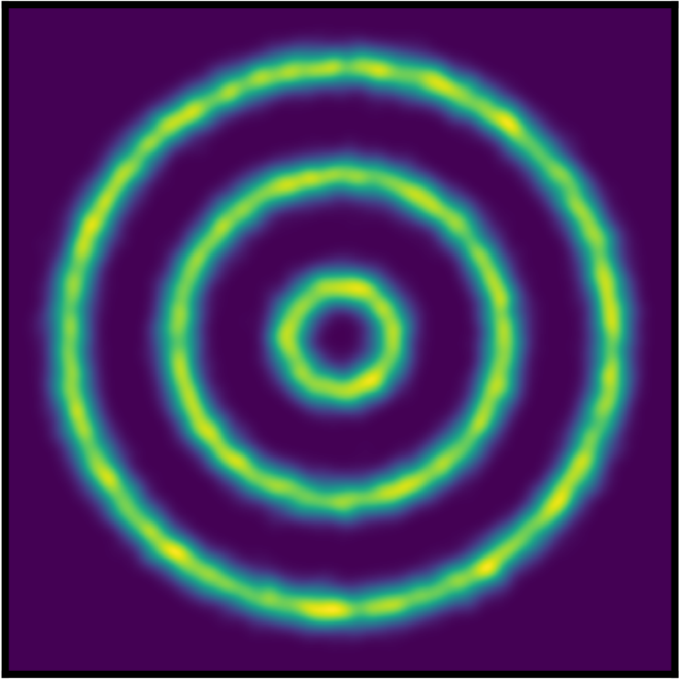
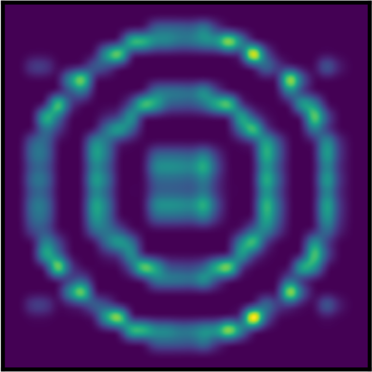
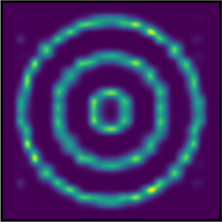
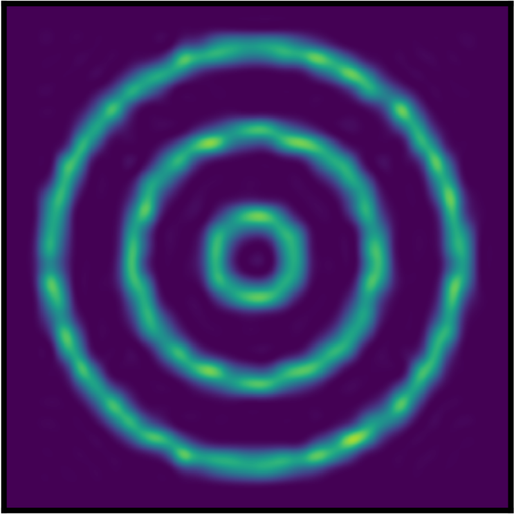
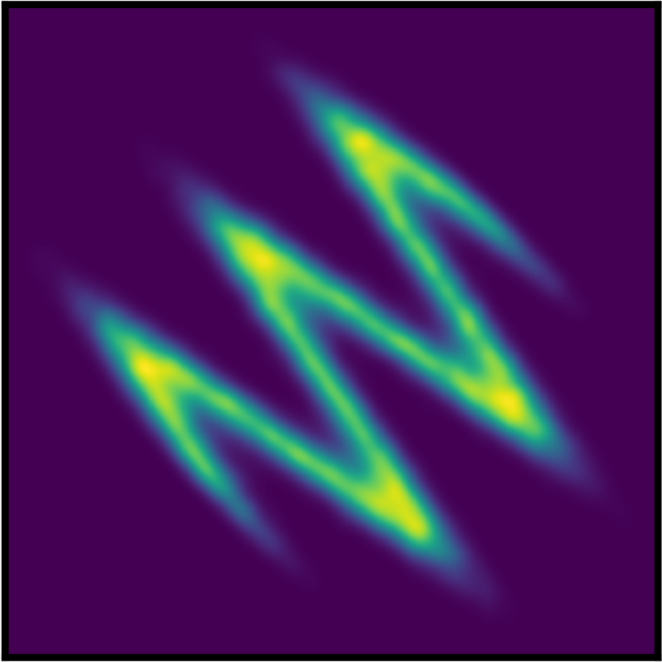
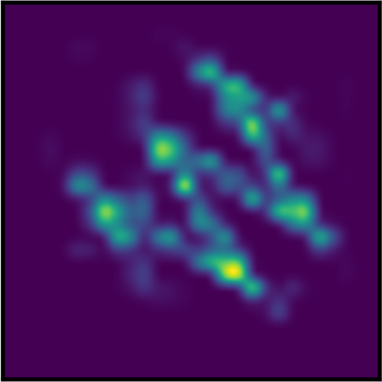
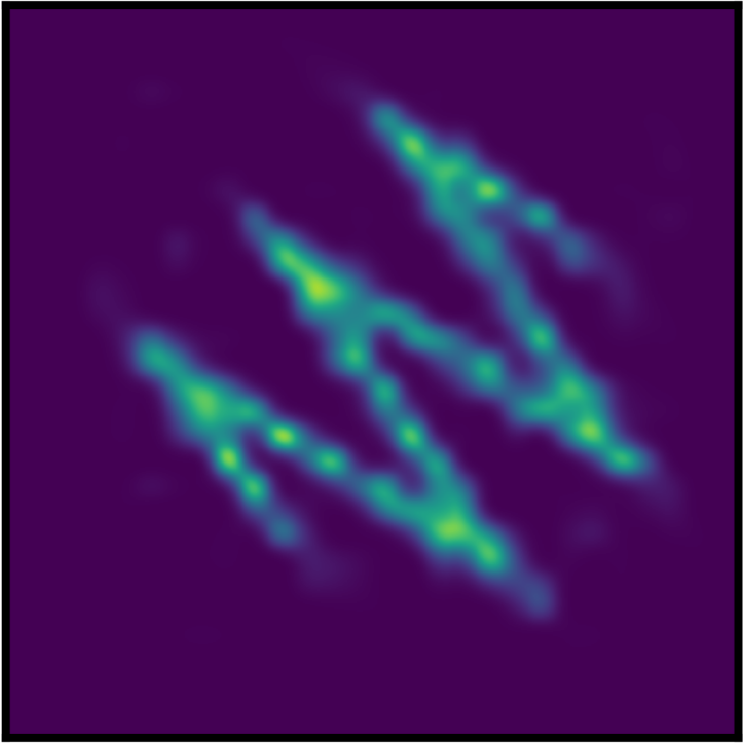
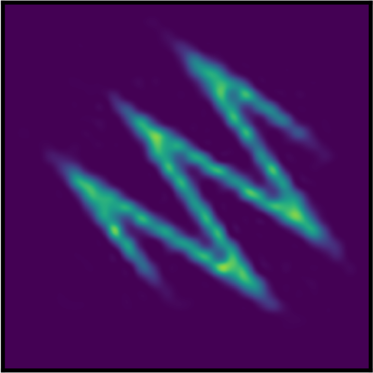
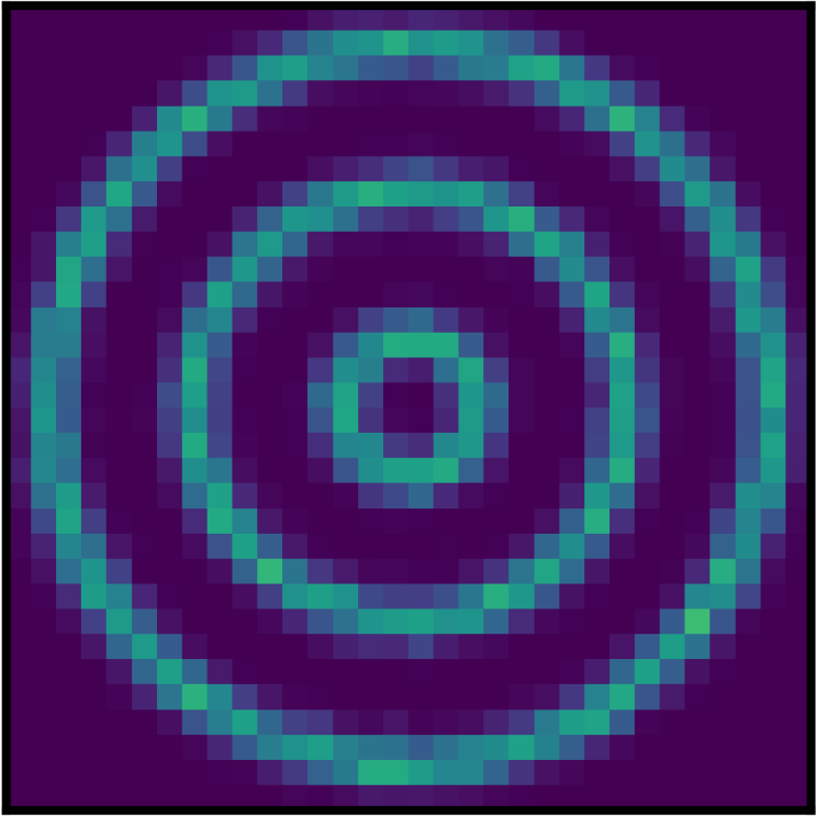
(a) GT

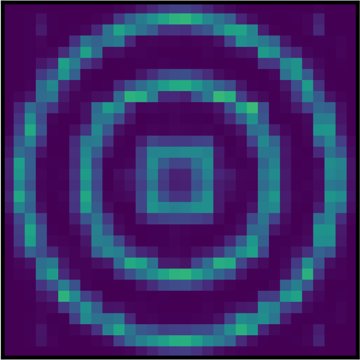
(b) MPC

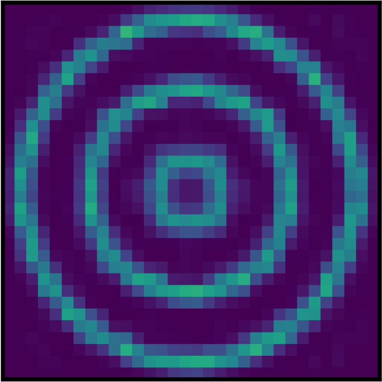
(c) MPC²

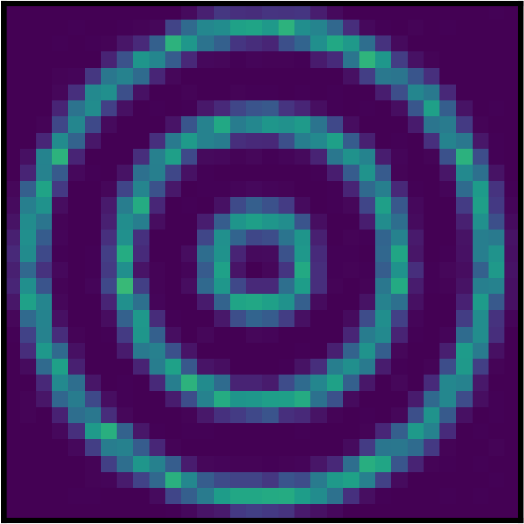
(d) NPC²

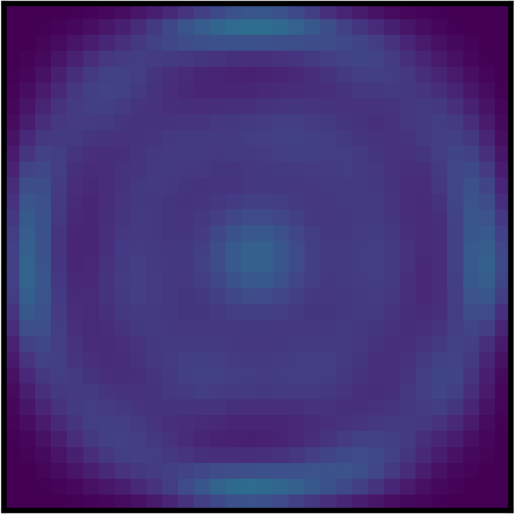
(e) MPC

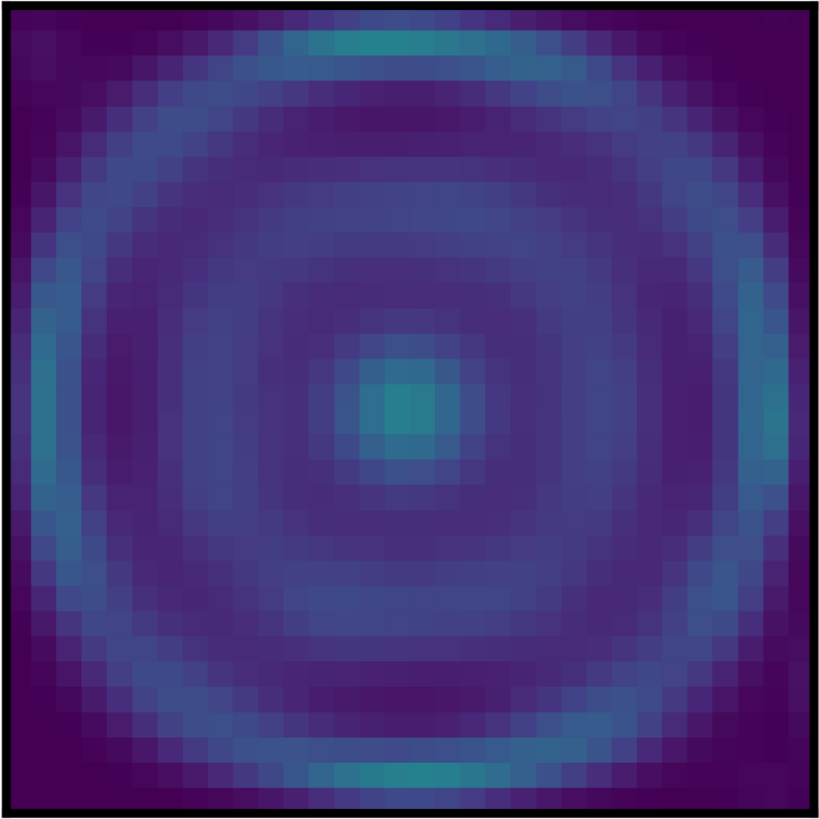
(f) MPC²

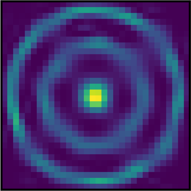
(g) NPC²

Figure 3: NPC²s are better estimators, especially with parameter-efficient input layers. Distribution estimated by monotonic PCs (MPC), squared monotonic PCs (MPC²) and NPC²s on 2D continuous (above) and discrete (below) data. On continuous data input layers compute splines (Eq. 11), while on discrete data they compute either categoricals (for MPC and MPC²), embeddings (for NPC²s) or Binomials. Secs. F.1 and F.2 shows log-likelihoods on also additional data.

4.2 Additional Related Works

Squared neural family (SNEFY) (Tsuchida et al., 2023) have been concurrently proposed as a class of models squaring the 2-norm of the output of a single-hidden-layer neural network. Under certain parametric conditions, SNEFYs can be re-normalized as to model a density function, but they do not guarantee tractable marginalization of any subset of variables as our NPC²s do, unless they encode a fully-factorized distribution, which would limit their expressiveness. Hence, SNEFYs can be employed in our NPC²s to model multivariate units in input layers with bounded scopes. The rich literature of PCs provides several algorithms to learn both the structure and the parameters of circuits (Poon & Domingos, 2011; Peharz et al., 2017; Di Mauro et al., 2021; Dang et al., 2021; Liu & Van den Broeck, 2021; Liu et al., 2023). However, in these works circuits are always assumed to be monotonic. A first work considering subtractions is Dennis (2016) which generalizes the ad-hoc constraints over Gaussian NMMs (Zhang & Zhang, 2005) to deep PCs over Gaussian inputs by constraining their structure and reparameterizing their sum weights. Shallow NMM represented as squared circuits have been investigated for low-dimensional categorical distributions in (Loconte et al., 2023). Circuit representations encoding probability generating functions allow negative coefficients, but in symbolic computational graphs (Zhang et al., 2021).

5 Experiments

We aim to answer to the following questions: (A) are NPC²s better distribution estimators than monotonic PCs? (B) how the increased model size given by squaring and the presence of negative parameters independently influence the expressivity of NPC²s? (C) how does the choice of input layers and the RG affect the performance of NPC²s? We perform several distribution estimation experiments on both synthetic and real-world data, and label the following paragraphs with letters denoting relevance to the above questions.

(A, B) Synthetic continuous data. Following Wenliang et al. (2019), we start by evaluating monotonic PCs and NPC²s on 2D density estimation tasks, as this allows us to gain an insight on the learned density functions. To disentangle the effect of squaring versus that of negative parameters, we also experiment with squared monotonic PCs (MPC²). We build both circuit structures from a trivial tree RG, see Sec. F.1 for experimental details and hyperparameters. We experiment with (possibly negative) splines as input layers for NPC²s, and enforce their non-negativity for monotonic PCs (see App. E). Fig. 3 shows that, while squaring benefits monotonic PCs, negative parameters in NPC²s are needed to better capture complex target densities.

		Power	Gas	Hepmass	M.BooNE	BSDS300
MADE		-3.08	3.56	-20.98	-15.59	148.85
RealNVP		0.17	8.33	-18.71	-13.84	153.28
MAF		0.24	10.08	-17.73	-12.24	154.93
NSF		0.66	13.09	-14.01	-9.22	157.31
Gaussian		-7.74	-3.58	-27.93	-37.24	96.67
EiNet-LRS		0.36	4.79	-22.46	-34.21	—
TTDE		0.46	8.93	-21.34	-28.77	143.30
MPC	(LT)	0.51	6.73	-22.06	-32.47	116.90
NPC2	(LT)	0.53	9.00	-20.66	-26.68	118.58
MPC	(BT)	0.57	5.56	-22.45	-32.11	123.30
NPC2	(BT)	0.62	10.98	-20.41	-26.92	128.38

Figure 4: NPC²s can be more expressive than monotonic PCs (MPCs). Best average log-likelihoods achieved by monotonic PCs ($+$) and NPC²s ($\pm^{2}$), built either from randomized linear tree (LT) or binary tree (BT) RGs (see Sec. F.3). The scatter plots (left) pairs log-likelihoods based on the number of units per layer $K$ (the higher the darker), differentiating PCs with Gaussian (G:blue) and splines (S:red) input layers. The table (right) shows our models’ best average test log-likelihoods and puts them in context with intractable (above) and tractable (below) models.

(C) Synthetic discrete data. We estimate the probability mass of the previous 2D datasets, now finitely-discretized (see Sec. F.2 for details) to better understand when negative parameters might bring little to no advantage if input layers are already expressive enough (Sec. 2). First, we experiment with (squared) monotonic PCs (resp. NPC²s) having input layers computing categoricals (resp. real-valued embeddings). Second, we employ the less flexible but more parameter-efficient Binomials instead. Sec. F.2 reports the hyperparameters. Fig. 3 shows that, while there is no clear advantage for NPC²s equipped with embeddings instead of MPC² with categoricals, in case of Binomials they can better capture the target distribution. This is because categoricals (resp. embeddings) already have enough parameters to capture “holes” in the probability mass function. However, Binomials introduce a strong inductive bias that might hinder learning. We believe this is the reason why, according to some preliminary results, we did not observe an improvement of NPC²s with respect to monotonic PCs on estimating image distributions.

(A, B, C) Multi-variate continuous data. Following Papamakarios et al. (2017), we evaluate deeper PCs for density estimation on five multivariate data sets (statistics are reported in Table F.1). We evaluate monotonic PCs and NPC²s in tensorized form built out of randomized linear tree RGs. That is, for some variable permutation, we construct a tree RG where each partition splits a region into a set of only one variable and recursively factorizes the rest. By doing so, we recover architectures similar to a BMs or TTDEs (see Sec. 4). Following Peharz et al. (2020b), we also experiment with randomized binary tree RGs whose partitions randomly split regions in half. Sec. F.3 details the experimental setting and hyperparameters. We compare against: a full covariance Gaussian, normalizing flows RealNVP (Dinh et al., 2017), MADE (Germain et al., 2015), MAF (Papamakarios et al., 2017) and NSF (Durkan et al., 2019), a monotonic PC with input layers encoding flows (EiNet-LRS) (Sidheekh et al., 2023), and TTDE (Novikov et al., 2021). Fig. 4 shows that NPC²s with Gaussian input layers generally achieve higher log-likelihoods than monotonic PCs on four data sets. Fig. F.3 shows similar results when comparing to squared monotonic PCs, thus providing evidence that negative parameters other than squaring contribute to the expressiveness of NPC²s. Binary tree RGs generally deliver better likelihoods than linear tree ones, especially on Gas, where NPC²s using them outperform TTDE, which uses a sophisticated Riemaniann optimization scheme.

(A) Distilling intractable models. Monotonic PCs have been used to approximate intractable models such as LLMs and perform exact inference in presence of logical constraints, such as for constrained text generation (Zhang et al., 2023). As generation performance is correlated with how well the LLM is approximated by a tractable model, we are interested in how NPC²s can better be the distillation target of a LLM such as GPT2, rather than monotonic PCs. Following Zhang et al. (2023), we minimize the KL divergence between GPT2 and our PCs on a dataset of sentences having bounded length (see Sec. F.4 for details). Since sentences are sequences of token variables, the architecture of tensorized circuits is built from a linear tree RG, thus corresponding to an inhomogeneous HMM in case of monotonic PCs (see Sec. B.4.1) while resembling a BM for NPC²s. Fig. 5 shows that NPC²s can scale and distill GPT2 more compactly than monotonic PCs, as they achieve log-likelihoods closer to the ones computed by GPT2 while generalizing similarly.

Figure 5: NPC²s ($\pm^{2}$) achieve higher log-likelihoods than monotonic PCs ($+$) on data sampled by GPT2, while generalizing similarly. We report the median and the area including 80% of runs by varying the size of layers $K$ and other hyperparameters (Sec. F.4). For comparison, the log-likelihood of GPT2 on the same training data is about $-52$ nats.

6 Discussion & Conclusion

With this work, we hope to popularize subtractive MMs via squaring as a simple and effective model class in the toolkit of tractable probabilistic modeling and reasoning that can rival traditional additive MMs. By casting them in the framework of circuits, we presented how to effectively represent and learn deep subtractive MMs such as NPC²s (Sec. 3) while showing how they can generalize other model classes such as PSD and tensor network models (Sec. 4). Our main theoretical result (Sec. 4.1) applies also to these models and justifies the increased performance we found in practice (Sec. 5). This work is the first to rigorously address representing and learning non-monotonic PCs in a general way, and opens up a number of future research directions. The first one is to retrieve a latent variable interpretation for NPC²s, as negative parameters in a non-monotonic PC invalidate the probabilistic interpretation of its sub-circuits (Peharz et al., 2017), making it not possible to learn its structure and parameters in classical ways (Sec. 4.2). Better ways to learn NPC²s, in turn, can benefit all applications in which PCs are widely used – from causal discovery (Wang et al., 2022) to variational inference (Shih & Ermon, 2020) and neuro-symbolic AI (Ahmed et al., 2022) – by making more compact and expressive distributions accessible. Finally, by connecting circuits with tensor networks for the first time, we hope to inspire works that carry over the advancements of one community to the other, such as better learning schemes (Stoudenmire & Schwab, 2016; Novikov et al., 2021), and more flexible ways to factorize high-dimensional tensors (Mari et al., 2023).

Reproducibility statement.

In App. F we include all the details about the experiments in Sec. 5. The source code, documentation and scripts needed to reproduce the results and figures of our experiments are available at https://github.com/anon-npc/squared-npcs.

Appendix A Circuits

Figure A.1: Computational units can be grouped into layers as to build a tensorized circuit. Sum units each parameterized by the rows of $\bm{\mathrm{W}}\in\mathbb{R}^{3\times 3}$ (left, in purple) form a sum layer parameterized by $\bm{\mathrm{W}}$ (right). Product units (left, in red) form an Hadamard product layer (right). Input units (left, in yellow) form an input layer computing the same functions (right)

In Sec. 3 we introduced circuits in a tensorized form. Here we instead present the definitions and properties of circuits as they are usually defined in the literature, which will be used in App. B.

Definition A.1 (Circuit (Choi et al., 2020; Vergari et al., 2021)).

A circuit $c$ is a parametrized computational graph over variables $\bm{\mathrm{X}}$ encoding a function $c(\bm{\mathrm{X}})$ and comprising three kinds of computational units: input, product, and sum. Each product or sum unit $n$ receives as inputs the outputs of other units, denoted with the set ${\mathsf{in}}(n)$. Each unit $n$ encodes a function $c_{n}$ defined as: (i) $f_{n}({\mathsf{sc}}(n))$ if $n$ is an input unit, where $f_{n}$ is a function over variables ${\mathsf{sc}}(n)\subseteq\bm{\mathrm{X}}$, called its scope, (ii) $\prod_{i\in{\mathsf{in}}(n)}c_{i}({\mathsf{sc}}(n_{i}))$ if $n$ is a product unit, and (iii) $\sum_{i\in{\mathsf{in}}(n)}w_{i}c_{i}({\mathsf{sc}}(c_{i}))$ if $n$ is a sum unit, with $w_{i}\in\mathbb{R}$ denoting the weighted sum parameters. The scope of a product or sum unit $n$ is the union of the scopes of its inputs, i.e., ${\mathsf{sc}}(n)=\bigcup_{i\in{\mathsf{in}}(n)}{\mathsf{sc}}(i)$.

Note that tensorized circuits (Def. 1) are circuits where each input (resp. product and sum) layer consists of scalar input (resp. product and sum) units. For example, Fig. A.1 shows how computational units are grouped into layers. A probabilistic circuit (PC) is defined as a circuit encoding a non-negative function. PCs that are smooth and decomposable (Def. A.2) enable computing the partition function and, more in general, performing variable marginalization efficiently (Prop. A.1).

Definition A.2 (Smoothness and decomposability (Darwiche & Marquis, 2002)).

A circuit is smooth if for every sum unit $n$, its input units depend all on the same variables, i.e, $\forall i,j\in{\mathsf{in}}(n)\colon{\mathsf{sc}}(i)={\mathsf{sc}}(j)$. A circuit is decomposable if the inputs of every product unit $n$ depend on disjoint sets of variables, i.e, $\forall i,j\in{\mathsf{in}}(n)\ i\neq j\colon{\mathsf{sc}}(i)\cap{\mathsf{sc}}(j)=\varnothing$.

Proposition A.1 (Tractability (Choi et al., 2020)).

Let $c$ be a smooth and decomposable circuit over variables $\bm{\mathrm{X}}$ whose input units can be integrated efficiently. Then for any $\bm{\mathrm{Z}}\subseteq\bm{\mathrm{X}}$ and $\bm{\mathrm{y}}$ an assignment to variables in $\bm{\mathrm{X}}\setminus\bm{\mathrm{Z}}$, the quantity $\int c(\bm{\mathrm{y}},\bm{\mathrm{z}})\,\mathrm{d}\bm{\mathrm{z}}$ can be computed exactly in time and space $\Theta(|c|)$, where $|c|$ denotes the size of the circuit, i.e., the number of connections in the computational graph.

The size of circuits in tensorized form is obtained by counting the number of connections between the scalar computational units (as detailed in Sec. A.1.1). Squaring circuits or their tensorized representation efficiently such that the resulting PC is smooth and decomposable (Def. A.2) requires the satisfaction of structured-decomposability, as showed in (Pipatsrisawat & Darwiche, 2008; Vergari et al., 2021).

Definition A.3 (Structured-decomposability (Pipatsrisawat & Darwiche, 2008; Darwiche, 2009)).

A circuit is structured-decomposable if (1) it is smooth and decomposable, and (2) any pair of product units $n,m$ having the same scope decompose their scope at their input units in the same way.

Note that shallow MMs are both decomposable and structured-decomposable. As anticipated in Sec. 3, the expressiveness of squared non-monotonic PCs that are also deterministic is the same as monotonic deterministic PCs, which are used for tractable maximum-a-posteriori (MAP) inference. We prove it formally in Sec. B.6 by leveraging the definition of determinism that we show in Def. A.5. Before that, we introduce the definition of support of a computational unit.

Definition A.4 (Support (Choi et al., 2020)).

The support of a computational unit $n$ over variables $\bm{\mathrm{X}}$ is defined as the set of value assignments to variables in $\bm{\mathrm{X}}$ such that the output of $n$ is non-zero, i.e., $\mathsf{supp}(n)=\{\bm{\mathrm{x}}\in\mathsf{val}(\bm{\mathrm{X}})\mid c_{n}(\bm{\mathrm{x}})\neq 0\}$, where $\mathsf{val}(\bm{\mathrm{X}})$ denotes the domain of variables $\bm{\mathrm{X}}$.

Definition A.5 (Determinism (Darwiche, 2001)).

A circuit $c$ is deterministic if for any sum unit $n\in c$ its inputs have disjoint support (Def. A.4), i.e., $\forall i,j\in{\mathsf{in}}(n),i\neq j\colon\mathsf{supp}(i)\cap\mathsf{supp}(j)=\varnothing$.

A.1 Tensorized Circuits

Def. 1 can be further generalized by introducing Kronecker product layers, which are the building blocks of other tensorized circuit architectures, such as randomized and tensorized sum-product networks (RAT-SPNs) (Peharz et al., 2020b), einsum networks (EiNets) (Peharz et al., 2020a).

Definition A.6 (Tensorized circuit).

A tensorized circuit $c$ is a parametrized computational graph encoding a function $c(\bm{\mathrm{X}})$ and comprising of three kinds of layers: input, product and sum. Each layer comprises computational units defined over the same set of variables, also called its scope, and every non-input layer receives input from one or more layers. The scope of each non-input layer is the union of the scope of its inputs, and the scope of the output layer computing $c(\bm{\mathrm{X}})$ is $\bm{\mathrm{X}}$. Each input layer $\bm{\mathrm{\ell}}$ has scope $\bm{\mathrm{Y}}\subseteq\bm{\mathrm{X}}$ and computes a collection of $K$ functions $f_{i}(\bm{\mathrm{Y}})\in\mathbb{R}$, i.e., $\bm{\mathrm{\ell}}$ outputs a $K$-dimensional vector. Each product layer $\bm{\mathrm{\ell}}$ computes either an Hadamard (or element-wise) or Kronecker product over the $N$ layers it receives as input, i.e., $\bm{\mathrm{\ell}}=\odot_{i=1}^{N}\bm{\mathrm{\ell}}_{i}$ or $\otimes_{i=1}^{N}\bm{\mathrm{\ell}}_{i}$, respectively. A sum layer with $S$ sum units and receiving input form a previous layer $\bm{\mathrm{\ell}}\in\mathbb{R}^{K}$, is parametrized by $\bm{\mathrm{W}}\in\mathbb{R}^{S\times K}$ and computes $\bm{\mathrm{W}}\bm{\mathrm{\ell}}$.

A.1.1 Size of Tensorized Circuits

The time and space complexity of evaluating a circuit is linear in its size. The size $|c|$ of a circuit $c$ (Def. A.1) is obtained by counting the number of input connections of each scalar product or sum unit. In other words, it is the number of edges in its computational graph.

If $c$ is a tensorized circuit, then its size is obtained by counting the number of connections in its non-tensorized form. Fig. A.1 shows part of a tensorized circuit and its non-tensorized form. For sum layers the number of scalar input connections is the size of its parameterization matrix, i.e., $S\cdot K$ if it is parameterized by $\bm{\mathrm{W}}\in\mathbb{R}^{S\times K}$. If $\bm{\mathrm{\ell}}$ is an Hadamard product layer computing $\bm{\mathrm{\ell}}=\odot_{i=1}^{N}\bm{\mathrm{\ell}}_{i}$, where each $\bm{\mathrm{\ell}}_{i}$ outputs a $K$-dimensional vector, then the number of its scalar input connections is $N\cdot K$. In case of Kronecker product layers as in the more general Def. A.6, i.e., $\bm{\mathrm{\ell}}=\otimes_{i=1}^{N}\bm{\mathrm{\ell}}_{i}$ where each $\bm{\mathrm{\ell}}_{i}$ outputs a $K$-dimensional vector, then the number of its scalar input connections is $K^{N+1}$.

A.2 Tractable Exact Sampling

Each sum unit in a monotonic PC can be interpreted as a finitely discrete latent variable that can assume as many values as the number of input connections (Peharz et al., 2017). As such, a monotonic PC can be seen as a hierarchical MM. This allows us to sample exactly from the modeled distribution by (1) recursively sampling latent variables until input units are reached, and (2) sampling observed variables from the distributions modeled by input units (Vergari et al., 2019a).

Such probabilistic interpretation of inner sum units for NPC²s is not possible, as they can output negative values. However, since NPC²s are smooth and decomposable (Def. A.2), they support efficient marginalization and hence conditioning (1). This allows us to still sample exactly from the modeled distribution via inverse transform sampling. That is, we choose a variable ordering $X_{1},X_{2},\ldots,X_{D}$ and sample them in an autoregressive fashion, i.e., $x_{1}\sim p(X_{1})$, $x_{2}\sim p(X_{2}\mid x_{1})$, $\ldots$, $x_{D}\sim p(X_{D}\mid x_{1},\ldots,x_{D-1})$, which is still linear in the number of variables.

Appendix B Proofs

B.1 Squaring Tensorized Circuits

Proposition B.1 (Correctness of Alg. 1).

Let $c$ be a tensorized structured-decomposable circuit (Def. 1 and Def. A.3), then Alg. 1 recursively constructs the layers of the squared tensorized PC $c^{2}$ such that $c^{2}$ is also structured-decomposable.

Proof.

The proof is by induction on the structure of $c$. Let $\bm{\mathrm{\ell}}$ be a sum layer having as input $\bm{\mathrm{\ell}}_{\mathsf{i}}$ and computing $\bm{\mathrm{W}}\bm{\mathrm{\ell}}_{\mathsf{i}}$, with $\bm{\mathrm{W}}\in\mathbb{R}^{S\times K}$ and $\bm{\mathrm{\ell}}_{\mathsf{i}}$ computing an output in $\mathbb{R}^{S}$. If $\bm{\mathrm{\ell}}$ is the last layer of $c$ (i.e., the output layer), then $S=1$ since $c$ outputs a scalar, and the squared layer $\bm{\mathrm{\ell}}^{2}$ must compute

$$\bm{\mathrm{\ell}}^{2}=(\bm{\mathrm{W}}\bm{\mathrm{\ell}}_{\mathsf{i}})\cdot(\bm{\mathrm{W}}\bm{\mathrm{\ell}}_{\mathsf{i}})=(\bm{\mathrm{W}}\otimes\bm{\mathrm{W}})(\bm{\mathrm{\ell}}_{\mathsf{i}}\otimes\bm{\mathrm{\ell}}_{\mathsf{i}})=(\bm{\mathrm{W}}\otimes\bm{\mathrm{W}})\bm{\mathrm{\ell}}_{\mathsf{i}}^{2},$$

which requires squaring the input layer $\bm{\mathrm{\ell}}_{\mathsf{i}}$. By inductive hypothesis the squared circuit having $\bm{\mathrm{\ell}}_{\mathsf{i}}^{2}$ as output layer is structured-decomposable, hence also the squared circuit having $\bm{\mathrm{\ell}}^{2}$ as output layer must be. If $\bm{\mathrm{\ell}}$ is a non-output sum layer, we still require computing the Kronecker product of its input layer. The squared layer $\bm{\mathrm{\ell}}^{2}$ is again a sum layer that outputs a $S^{2}$-dimensional vector, i.e.,

$$\bm{\mathrm{\ell}}^{2}=\bm{\mathrm{\ell}}\otimes\bm{\mathrm{\ell}}=\left(\bm{\mathrm{W}}\bm{\mathrm{\ell}}_{\mathsf{i}}\right)\otimes\left(\bm{\mathrm{W}}\bm{\mathrm{\ell}}_{\mathsf{i}}\right)=(\bm{\mathrm{W}}\otimes\bm{\mathrm{W}})(\bm{\mathrm{\ell}}_{\mathsf{i}}\otimes\bm{\mathrm{\ell}}_{\mathsf{i}})=(\bm{\mathrm{W}}\otimes\bm{\mathrm{W}})\bm{\mathrm{\ell}}_{\mathsf{i}}^{2}$$

via mixed-product property (L11-15 in Alg. 1). Let $\bm{\mathrm{\ell}}$ be a binary Hadamard product layer computing $\bm{\mathrm{\ell}}_{\mathsf{i}}\odot\bm{\mathrm{\ell}}_{\mathsf{ii}}$ for input layers $\bm{\mathrm{\ell}}_{\mathsf{i}},\bm{\mathrm{\ell}}_{\mathsf{ii}}$ each computing a $K$-dimensional vector. Then, the squared layer $\bm{\mathrm{\ell}}^{2}$ computes the Hadamard product between $K^{2}$-dimensional vectors, i.e.,

$$\bm{\mathrm{\ell}}^{2}=(\bm{\mathrm{\ell}}_{\mathsf{i}}\odot\bm{\mathrm{\ell}}_{\mathsf{ii}})\otimes(\bm{\mathrm{\ell}}_{\mathsf{i}}\odot\bm{\mathrm{\ell}}_{\mathsf{ii}})=(\bm{\mathrm{\ell}}_{\mathsf{i}}\otimes\bm{\mathrm{\ell}}_{\mathsf{i}})\odot(\bm{\mathrm{\ell}}_{\mathsf{ii}}\otimes\bm{\mathrm{\ell}}_{\mathsf{ii}})=\bm{\mathrm{\ell}}_{\mathsf{i}}^{2}\odot\bm{\mathrm{\ell}}_{\mathsf{ii}}^{2}$$

via mixed-product property with respect to the Hadamard product. By inductive hypothesis $\bm{\mathrm{\ell}}_{\mathsf{i}}^{2}$ and $\bm{\mathrm{\ell}}_{\mathsf{ii}}^{2}$ are the output layers of structured-decomposable circuits depending on a disjoint sets of variables. As such, the circuit having $\bm{\mathrm{\ell}}^{2}$ as output layer maintains structured-decomposability (L6-9 in Alg. 1). For the base case we consider the squaring of an input layer $\bm{\mathrm{\ell}}$ that computes $K$ functions $f_{i}$ over some variables $\bm{\mathrm{Y}}\subseteq\bm{\mathrm{X}}$. We replace $\bm{\mathrm{\ell}}$ with its squaring $\bm{\mathrm{\ell}}^{2}$ which encodes the products $f_{i}(\bm{\mathrm{Y}})f_{j}(\bm{\mathrm{Y}})$, $1\leq i,j\leq K$, by introducing $K^{2}$ functions $g_{ij}$ such that $g_{ij}(\bm{\mathrm{Y}})=f_{i}(\bm{\mathrm{Y}})f_{j}(\bm{\mathrm{Y}})$ (L2-4 in Alg. 1).

Squaring Kronecker product layers. In the case of $\bm{\mathrm{\ell}}$ being a binary Kronecker product layer instead as in the more general Def. A.6, then the squared layer $\bm{\mathrm{\ell}}^{2}$ computes the Kronecker product between $K^{2}$-dimensional vectors up to a permutation of the entries, i.e.,

$$\bm{\mathrm{\ell}}^{2}=(\bm{\mathrm{\ell}}_{\mathsf{i}}\otimes\bm{\mathrm{\ell}}_{\mathsf{ii}})\otimes(\bm{\mathrm{\ell}}_{\mathsf{i}}\otimes\bm{\mathrm{\ell}}_{\mathsf{ii}})=\bm{\mathrm{R}}\left((\bm{\mathrm{\ell}}_{\mathsf{i}}\otimes\bm{\mathrm{\ell}}_{\mathsf{i}})\otimes(\bm{\mathrm{\ell}}_{\mathsf{ii}}\otimes\bm{\mathrm{\ell}}_{\mathsf{ii}})\right)=\bm{\mathrm{R}}\left(\bm{\mathrm{\ell}}_{\mathsf{i}}^{2}\otimes\bm{\mathrm{\ell}}_{\mathsf{ii}}^{2}\right),$$ (6)

by introducing a $K^{4}\times K^{4}$ permutation matrix $\bm{\mathrm{R}}$ whose rows are all zeros except for one entry set to 1, which reorders the entries of $\bm{\mathrm{\ell}}_{\mathsf{i}}^{2}\otimes\bm{\mathrm{\ell}}_{\mathsf{ii}}^{2}$ as to recover the equality in Eq. 6. Note that such permutation maintains decomposability (Def. A.2), and its application can be computed by a sum layer having $\bm{\mathrm{R}}$ as fixed parameters. Moreover, by inductive hypothesis, the squaring circuit having $\bm{\mathrm{\ell}}^{2}$ as output layer is still structured-decomposable. Finally, Alg. B.2 generalizes Alg. 1 as to support the squaring of Kronecker product layers as showed above (L10-11 in Alg. B.2). ∎

Algorithm B.2 $\textsf{squareTensorizedCircuit}(\bm{\mathrm{\ell}},\mathcal{R})$

Input: A tensorized circuit (Def. A.6) having output layer $\bm{\mathrm{\ell}}$ and defined on a tree RG rooted by $\mathcal{R}$.
Output: The tensorized squared circuit defined on the same tree RG having $\bm{\mathrm{\ell}}^{2}$ as output layer computing $\bm{\mathrm{\ell}}\otimes\bm{\mathrm{\ell}}$.

1:if $\bm{\mathrm{\ell}}$ is an input layer then

2:     $\bm{\mathrm{\ell}}$ computes $K$ functions $f_{i}(\mathcal{R})$

3:     return An input layer $\bm{\mathrm{\ell}}^{2}$ computing all $K^{2}$

4:          product combinations $f_{i}(\mathcal{R})f_{j}(\mathcal{R})$

5:else if $\bm{\mathrm{\ell}}$ is a product layer then

6:     $\{(\bm{\mathrm{\ell}}_{\textsf{i}},\mathcal{R}_{\textsf{i}}),\ (\bm{\mathrm{\ell}}_{\textsf{ii}},\mathcal{R}_{\textsf{ii}})\}\leftarrow\textsf{getInputs}(\bm{\mathrm{\ell}},\mathcal{R})$

7:     $\bm{\mathrm{\ell}}_{\textsf{i}}^{2}\leftarrow\textsf{squareTensorizedCircuit}(\bm{\mathrm{\ell}}_{\textsf{i}},\mathcal{R}_{\textsf{i}})$

8:     $\bm{\mathrm{\ell}}_{\textsf{ii}}^{2}\leftarrow\textsf{squareTensorizedCircuit}(\bm{\mathrm{\ell}}_{\textsf{ii}},\mathcal{R}_{\textsf{ii}})$

9:     if $\bm{\mathrm{\ell}}=\bm{\mathrm{\ell}}_{\textsf{i}}\odot\bm{\mathrm{\ell}}_{\textsf{ii}}$ then return $\bm{\mathrm{\ell}}_{\textsf{i}}^{2}\odot\bm{\mathrm{\ell}}_{\textsf{ii}}^{2}$

10:     else return $\bm{\mathrm{R}}\left(\bm{\mathrm{\ell}}_{\textsf{i}}^{2}\otimes\bm{\mathrm{\ell}}_{\textsf{ii}}^{2}\right)$, where $\bm{\mathrm{R}}$ is

11:      a permutation matrix (see proof of Prop. B.1)      

12:else$\triangleright$ $\bm{\mathrm{\ell}}$ is a sum layer

13:     $\{(\bm{\mathrm{\ell}}_{\mathsf{i}},\mathcal{R})\}\leftarrow\textsf{getInputs}(\bm{\mathrm{\ell}},\mathcal{R})$

14:     $\bm{\mathrm{\ell}}_{\mathsf{i}}^{2}\leftarrow\textsf{squareTensorizedCircuit}(\bm{\mathrm{\ell}}_{\mathsf{i}},\mathcal{R})$

15:     $\bm{\mathrm{W}}\in\mathbb{R}^{S\times K}\leftarrow\textsf{getParameters}(\bm{\mathrm{\ell}})$

16:     $\bm{\mathrm{W}}^{\prime}\in\mathbb{R}^{S^{2}\times K^{2}}\leftarrow\bm{\mathrm{W}}\otimes\bm{\mathrm{W}}$

17:     return $\bm{\mathrm{W}}^{\prime}\bm{\mathrm{\ell}}_{\mathsf{i}}^{2}$

B.2 Tractable Marginalization of NPC²s

Proposition 1.

Let $c$ be a tensorized structured-decomposable circuit where the products of functions computed by each input layer can be tractably integrated. Any marginalization of $c^{2}$ obtained via Alg. 1 requires time and space $\mathcal{O}(L\cdot M^{2})$.

Proof.

Given $c$ by hypothesis, Prop. B.1 ensures that the PC built via Alg. 1 computes $c^{2}$ and is defined on the same tree RG (Def. 2) of $c$. As such, $c^{2}$ is structured-decomposable and hence also smooth and decomposable (see Def. A.3). Now, we make an argument about $c$ and $c^{2}$ in their non-tensorized form (Def. A.1) as to leverage Prop. A.1 for tractable marginalization later. The size of $c$ is $|c|\in\mathcal{O}(L\cdot M)$, where $L$ is the number of layers and $M$ the maximum number of scalar input connections of each layer in $c$ (see Sec. A.1.1 for details). The size of $c^{2}$ is therefore $|c^{2}|\in\mathcal{O}(L\cdot M^{2})$, since Alg. 1 squares the output dimension of each layer as well as the size of the parameterization matrix of each sum layer. Since $c^{2}$ is smooth and decomposable and the functions computed by its input layers can be tractably integrated, then Prop. A.1 ensures we can marginalize any subset of variables in time and space $|c^{2}|\in\mathcal{O}(L\cdot M^{2})$. ∎

B.3 Representing PSD models within the language of NPC²s

Proposition 2.

A PSD model with kernel function $\kappa$, defined over $d$ data points, and parameterized by a PSD matrix $\bm{\mathrm{A}}$, can be represented as a mixture of squared NMMs (hence NPC²s) in time $\mathcal{O}(d^{3})$.

Proof.

The PSD model computes a non-negative function $f(\bm{\mathrm{x}};\bm{\mathrm{A}},\bm{\mathrm{\kappa}})=\bm{\mathrm{\kappa}}(\bm{\mathrm{x}})^{\top}\bm{\mathrm{A}}\bm{\mathrm{\kappa}}(\bm{\mathrm{x}})$, where $\bm{\mathrm{\kappa}}(\bm{\mathrm{x}})=[\kappa(\bm{\mathrm{x}},\bm{\mathrm{x}}^{(1)}),\ldots,\kappa(\bm{\mathrm{x}},\bm{\mathrm{x}}^{(d)})]\in\mathbb{R}^{d}$, with data points $\bm{\mathrm{x}}^{(1)},\ldots,\bm{\mathrm{x}}^{(d)}$, and $\bm{\mathrm{A}}\in\mathbb{R}^{d\times d}$ is PSD. Let $\bm{\mathrm{A}}=\sum_{i=1}^{r}\lambda_{i}\bm{\mathrm{u}}_{i}\bm{\mathrm{u}}_{i}^{\top}$ be the eigendecomposition of $\bm{\mathrm{A}}$ with rank $r$. Then we can rewrite $f(\bm{\mathrm{x}};\bm{\mathrm{A}},\bm{\mathrm{\kappa}})$ as

$$f(\bm{\mathrm{x}};\bm{\mathrm{A}},\bm{\mathrm{\kappa}})=\bm{\mathrm{\kappa}}(\bm{\mathrm{x}})^{\top}\left(\sum\nolimits_{i=1}^{r}\lambda_{i}\bm{\mathrm{u}}_{i}\bm{\mathrm{u}}_{i}^{\top}\right)\bm{\mathrm{\kappa}}(\bm{\mathrm{x}})=\sum\nolimits_{i=1}^{r}\lambda_{i}\left(\bm{\mathrm{u}}_{i}^{\top}\bm{\mathrm{\kappa}}(\bm{\mathrm{x}})\right)^{2},$$

where $\lambda_{i}>0$ since $\bm{\mathrm{A}}$ is PSD. Therefore, such PSD model can be represented as a monotonic mixture of $r\leq d$ squared NMMs (Eq. 2), whose $d$ components computing $\bm{\mathrm{\kappa}}(\bm{\mathrm{x}})$ are shared. The eigendecomposition of $\bm{\mathrm{A}}$ can be done in time $\mathcal{O}(d^{3})$, and materializing each squared NMMs (e.g., as in Fig. 1) requires space $\mathcal{O}(d^{2})$. Furthermore, note that if $\bm{\mathrm{A}}=\bm{\mathrm{u}}\bm{\mathrm{u}}^{\top}$ is a rank-1 matrix, then $f(\bm{\mathrm{x}};\bm{\mathrm{A}},\bm{\mathrm{\kappa}})=\left(\bm{\mathrm{u}}^{\top}\bm{\mathrm{\kappa}}(\bm{\mathrm{x}})\right)$² is exactly a squared NMM whose $d$ components compute $\bm{\mathrm{\kappa}}(\bm{\mathrm{x}})$. ∎

B.4 Relationship with Tensor Networks

In this section, we detail the construction of a tensorized structured-decomposable circuit (Def. 1) that is equivalent to a matrix product state (MPS) tensor network (Pérez-García et al., 2007), as we mention in Sec. 4. As such, the application of the Born rule as to retrieve a probabilistic model called Born machine (BM) (Glasser et al., 2019) is equivalent to squaring the equivalent circuit (Sec. 3).

Proposition 3.

A BM encoding $D$-dimensional tensor with $m$ states by squaring a rank $r$ MPS can be exactly represented as a structured-decomposable NPC² in $\mathcal{O}(D\cdot k^{4})$ time and space, with $k\leq\min\{r^{2},mr\}$.

Proof.

We prove it constructively, by using a similar transformation used by Glasser et al. (2019) to represent a non-negative MPS factorization as an hidden Markov model (HMM). Let $\bm{\mathrm{X}}=\{X_{1},\ldots,X_{D}\}$ be a set of discrete variables each taking values in $\{1,\ldots,m\}$. Let $\mathcal{T}$ be a tensor with $D$ $m$-dimensional indices. Given an assignment $\bm{\mathrm{x}}=\langle x_{1},\ldots,x_{D}\rangle$ to $\bm{\mathrm{X}}$, we factorize $\mathcal{T}$ via a rank $r$ MPS factorization, i.e.,

$$\mathcal{T}[x_{1},\ldots,x_{D}]=\sum_{i_{1}=1}^{r}\sum_{i_{2}=1}^{r}\cdots\sum_{i_{D-1}=1}^{r}\bm{\mathrm{A}}_{1}[x_{1},i_{1}]\bm{\mathrm{A}}_{2}[x_{2},i_{1},i_{2}]\cdots\bm{\mathrm{A}}_{D}[x_{D},i_{D-1}]$$ (7)

where $\bm{\mathrm{A}}_{1},\bm{\mathrm{A}}_{D}\in\mathbb{R}^{m\times r}$ and $\bm{\mathrm{A}}_{j}\in\mathbb{R}^{m\times r\times r}$ with $1<j<D$, for indices $\{i_{1},\ldots,i_{D-1}\}$ and denoting indexing with square brackets. To reduce $\mathcal{T}$ to being computed by a tensorized structured-decomposable circuit $c$, i.e., such that $c(\bm{\mathrm{x}})=\mathcal{T}[x_{1},\ldots,x_{D}]$ for any $\bm{\mathrm{x}}$, we perform the following construction. First, we perform a CANDECOMP/PARAFAC (CP) decomposition (Kolda & Bader, 2009) of each $\bm{\mathrm{A}}_{j}$ with $1<j<D$, i.e.,

$$\bm{\mathrm{A}}_{j}[x_{j},i_{j-1},i_{j}]=\sum_{s_{j}=1}^{k}\bm{\mathrm{B}}_{j}[i_{j-1},s_{j}]\bm{\mathrm{V}}_{j}[x_{j},s_{j}]\bm{\mathrm{C}}_{j}[i_{j},s_{j}]$$

where $k\leq\min\{r^{2},mr\}$ is the maximum rank of the decomposition, and $\bm{\mathrm{V}}_{j}\in\mathbb{R}^{m\times k}$, $\bm{\mathrm{B}}_{j}\in\mathbb{R}^{r\times k}$, $\bm{\mathrm{C}}_{j}\in\mathbb{R}^{r\times k}$. Then, we “contract” each $\bm{\mathrm{C}}_{j}$ with $\bm{\mathrm{B}}_{j+1}$ by computing

$$\bm{\mathrm{W}}_{j}[s_{j},s_{j+1}]=\sum_{i_{j}=1}^{r}\bm{\mathrm{C}}_{j}[i_{j},s_{j}]\bm{\mathrm{B}}_{j+1}[i_{j},s_{j+1}]$$

with $\bm{\mathrm{W}}_{j}\in\mathbb{R}^{k\times k}$ for $1<j<D-1$. In addition, we “contract” $\bm{\mathrm{C}}_{D-1}$ with $\bm{\mathrm{A}}_{D}$ by computing

$$\bm{\mathrm{V}}_{D}[x_{D},s_{D-1}] =\sum_{i_{D-1}=1}^{r}\bm{\mathrm{C}}_{D-1}[i_{D-1},s_{D-1}]\bm{\mathrm{A}}_{D}[x_{D},i_{D-1}].$$

In addition, for notation clarity we rename $\bm{\mathrm{B}}_{2}$ with $\bm{\mathrm{W}}_{1}$ and $\bm{\mathrm{A}}_{1}$ with $\bm{\mathrm{V}}_{1}$. By doing so, we can rewrite Eq. 7 as a sum with indices $\{s_{2},\ldots,s_{D-1}\}$ over products, i.e.,

$$\mathcal{T}[x_{1},\ldots,x_{D}]= \sum_{i_{1}=1}^{r}\bm{\mathrm{V}}_{1}[x_{1},i_{1}]\sum_{s_{2}=1}^{k}\bm{\mathrm{W}}_{2}[i_{1},s_{2}]\bm{\mathrm{V}}[x_{2},s_{2}]$$

$$\cdots \sum_{s_{D-1}=1}^{k}\bm{\mathrm{W}}_{D-2}[s_{D-2},s_{D-1}]V_{D-1}[x_{D-1},s_{D-1}]V_{D}[x_{D},s_{D-1}]$$

Fig. B.1 shows an example of such MPS factorization via CP decompositions. We see that we can encode the products over the same indices using a Hadamard product layers, and summations over indices $\{s_{2},\ldots,x_{D-1}\}$ with sum layers parameterized by the $\bm{\mathrm{W}}_{j}$. More precisely, the sum layers that sum over $s_{2}$ and $s_{D-1}$ are parameterized by matrices of ones. Each $\bm{\mathrm{V}}_{j}$ with $1\leq j\leq D$ is instead encoded by an input layer depending on the variable $X_{j}$ and computing $k$ functions $f_{l}(X_{j})$ such that $f_{l}(x_{j})=\bm{\mathrm{V}}_{j}[x_{j},l]$ with $1\leq j\leq k$. The tensorized circuit constructed in this way is structured-decomposable, as it is defined on a linear tree RG (e.g., Fig. 2) induced by the variable ordering implicitly stated by the MPS factorization (Eq. 7, see Sec. B.4 for details). Fig. B.2 shows the circuit representation corresponding to the MPS reported in Fig. 1(b).

Finally, note that the number of parameters of such tensorized circuit correspond to the size of all $\bm{\mathrm{W}}_{j}$ and $\bm{\mathrm{V}}_{j}$ introduced above, i.e., $\mathcal{O}(D\cdot k^{2})$ where $k\leq\min\{r^{2},mr\}$. Moreover, the CP decompositions at the beginning can be computed using iterative methods whose iterations require polynomial time (Kolda & Bader, 2009). To retrieve an equivalent BM, we can square the circuit constructed in this way using Alg. 1, which results in a circuit having size $\mathcal{O}(D\cdot k^{4})$ (see Prop. B.1).

∎

(a)

(b)

(c)

Figure B.1: Further decomposing a matrix product state (MPS) via CP decompositions. Tensor networks are represented using the Penrose graphical notation, where circles denote tensors and their connections denote summations over shared indices, and variables $X_{1},X_{2},X_{3},X_{4}$ are input indices. Given a MPS (a), we perform a CP decomposition of $\bm{\mathrm{A}}_{2}$ and $\bm{\mathrm{A}}_{3}$ (b). Red edges denote additional indices given by the CP decompositions. Then, we rename $\bm{\mathrm{A}}_{1}$ with $\bm{\mathrm{V}}_{1}$, $\bm{\mathrm{B}}_{2}$ with $\bm{\mathrm{W}}_{1}$. Finally, we contract $\bm{\mathrm{C}}_{2}$ with $\bm{\mathrm{B}}_{3}$, and $\bm{\mathrm{C}}_{3}$ with $\bm{\mathrm{V}}_{4}$ resulting in tensors $\bm{\mathrm{W}}_{2}$ and $\bm{\mathrm{V}}_{4}$, respectively (c). Fig. B.2 shows the tensorized circuit corresponding to such tensor network.

(a)

(b)

Figure B.2: Matrix product states (MPS) as structured-decomposable circuits. The decomposed MPS over three variables showed in Fig. 1(c) can be immediately represented as a tensorized structured-decomposable circuit (a) defined on a linear tree RG (b, matching the colors of layers) having Hadamard product layers and sum layers parameterized by $\bm{\mathrm{W}}_{1},\bm{\mathrm{W}}_{2}$ and a row vector of ones $\mathbf{1}$. Each input layer maps $x_{1},x_{2},x_{3},x_{3}$ to rows in $\bm{\mathrm{V}}_{1},\bm{\mathrm{V}}_{2},\bm{\mathrm{V}}_{3},\bm{\mathrm{V}}_{4}$, respectively.

B.4.1 Relationship with Hidden Markov Models

MPS tensor networks where each tensor $\bm{\mathrm{A}}_{i}$ is non-negative can be seen as inhomogeneous hidden Markov models (HMMs) as showed by Glasser et al. (2019), i.e., where latent state and emitting transitions do not necessarily share parameters. As such, the tensorized structured-decomposable circuit $c$ that is equivalent to a MPS (see Sec. B.4) is also an inhomogenous HMM if $c$ is monotonic.

In Sec. 5 we experiment with a tensorized monotonic PC that is an inhomogenous HMM to distill a large language model, as to leverage the sequential structure of the sentences. We compare it against a NPC² that is the squaring of a MPS (also called Born machine (Glasser et al., 2019)) or, equivalently, the squaring of an inhomogenous HMM-like whose parameters can be negative.

B.5 Exponential Separation

Theorem 1.

There is a class of non-negative functions $\mathcal{F}$ over variables $\bm{\mathrm{X}}$ that can be compactly represented as shallow squared NMMs (and hence squared non-monotonic PCs) but for which the smallest structured-decomposable monotonic PC computing any $F\in\mathcal{F}$ has size $2^{\Omega(|\bm{\mathrm{X}}|)}$.

Proof.

For the proof of 1, we start by constructing $\mathcal{F}$ by introducing a variant of the unique disjointness (UDISJ) problem, which seems to have first been introduced by De Wolf (2003). The variant we consider here is defined over graphs, as detailed in the following definition.

Definition B.1 (Unique disjointness function).

Consider an undirected graph $G=(V,E)$, where $V$ denotes its vertices and $E$ its edges. To every vertex $v\in V$ we associate a Boolean variable $X_{v}$ and let $\bm{\mathrm{X}}_{V}=\{X_{v}\mid v\in V\}$ be the set of all these variables. The unique disjointness function of $G$ is defined as

$$\mathsf{UDISJ}_{G}(\bm{\mathrm{X}}_{v}):=\left(1-\sum_{uv\in E}X_{u}X_{v}\right)^{2}.$$ (8)

The UDISJ function as a non-monotonic circuit. We will construct $\mathcal{F}$ as the class of functions $\mathsf{UDISJ}_{G}$ for graphs $G\in\mathcal{G}$, where $\mathcal{G}$ is a family of graphs that we will choose later. Regardless of the way the class $\mathcal{G}$ is picked, we can compactly represent $\mathsf{UDISJ}_{G}$ as a squared structured-decomposable (Def. A.3) and non-monotonic circuit as follows. First, we represent the function $c(\bm{\mathrm{X}}_{V})=1-\sum_{uv\in E}X_{u}X_{v}$ as sum unit computing $1\cdot a(\bm{\mathrm{X}}_{V})+(-1)\cdot b(\bm{\mathrm{X}}_{V})$ where

• $a$ is a circuit gadget that realizes an unnormalized uniform distribution over the domain of variables in $\bm{\mathrm{X}}_{V}$, i.e., $a(\bm{\mathrm{X}}_{V})=\prod_{v\in V}(\mathbbm{1}\!\left\{X_{v}=0\right\}+\mathbbm{1}\!\left\{X_{v}=1\right\})$ where $\mathbbm{1}\!\left\{X_{v}=0\right\}$ (resp. $\mathbbm{1}\!\left\{X_{v}=1\right\}$) is an indicator function that outputs $1$ when $X_{v}$ is set to 0 (resp. 1);

• $b$ is another sum unit whose inputs are product units over the input units $\mathbbm{1}\!\left\{X_{u}=1\right\},\mathbbm{1}\!\left\{X_{v}=1\right\}$ if there is an edge $uv$ in $G$, i.e., $b(\bm{\mathrm{X}}_{V})=\sum_{uv\in E}\mathbbm{1}\!\left\{X_{u}=1\right\}\cdot\mathbbm{1}\!\left\{X_{v}=1\right\}$.

Note that $b$ may not be smooth, but we can easily smooth it by adding to every product an additional input that is a circuit similar to $a$ that outputs $1$ for any input $\bm{\mathrm{X}}_{\overline{uv}}$, where $\bm{\mathrm{X}}_{\overline{uv}}=\bm{\mathrm{X}}_{V}\setminus\{X_{u},X_{v}\}$. Since $c$ is structured-decomposable (Def. A.3), we can easily multiply it with itself to realize $c^{2}$ that would be still a structured-decomposable circuit whose size is polynomially bounded as $|c^{2}|\in\mathcal{O}(|c|^{2})$ (Vergari et al., 2021). In particular, in this case we have that $|c|$ is a polynomial in the number of variables (or vertices) $|\bm{\mathrm{X}}_{V}|$ by the construction above. Furthermore, note that $c^{2}$ is non-monotonic as one of its sum unit has negative parameters (i.e., $-1$) to encode the subtraction in Eq. 8.

The lower bound for monotonic circuits. To prove the exponential lower bound for monotonic circuits in 1, we will use an approach that has been used in several other works (Martens & Medabalimi, 2014; de Colnet & Mengel, 2021). This approach is based on representing a decomposable circuit (and hence a structured-decomposable one) as a shallow mixture whose components are balanced products, as formalized next.

Definition B.2.

Let $\bm{\mathrm{X}}$ be a set of variables. A balanced decomposable product over $\bm{\mathrm{X}}$ is a function from $\bm{\mathrm{X}}$ to $\mathbb{R}$ that can be written as $f(\bm{\mathrm{Y}})\times h(\bm{\mathrm{Z}})$ where $(\bm{\mathrm{Y}},\bm{\mathrm{Z}})$ is a partitioning of $\bm{\mathrm{X}}$, $f$ and $h$ are functions to $\mathbb{R}$ and $|\bm{\mathrm{X}}|/3\leq|\bm{\mathrm{Y}}|\leq 2|\bm{\mathrm{X}}|/3$.

Theorem B.1 (Martens & Medabalimi (2014)).

Let $F$ be a non-negative function over Boolean variables $\bm{\mathrm{X}}$ computed by a smooth and decomposable circuit $c$. Then, $F$ can be written as a sum of $N$ balanced decomposable products (Def. B.2) over $\bm{\mathrm{X}}$, with $N\leq|c|$ in the form

$$F(\bm{\mathrm{X}})=\sum_{k=1}^{N}f_{k}(\bm{\mathrm{Y}}_{k})\times h_{k}(\bm{\mathrm{Z}}_{k}),$$

where $(\bm{\mathrm{Y}}_{k},\bm{\mathrm{Z}}_{k})$ is partitioning of $\bm{\mathrm{X}}$ for $1\leq k\leq N$. If $c$ is structured-decomposable, the $N$ partitions $\{(\bm{\mathrm{Y}}_{k},\bm{\mathrm{Z}}_{k})\}_{k=1}^{N}$ are all identical. Moreover, if $c$ is monotonic, then all $f_{k},h_{k}$ only compute non-negative values.

Intuitively, Thm. B.1 tells us that to lower bound the size of $c$ we can lower bound $N$. To this end, we first encode the UDISJ function (Eq. 8) as a sum of $N$ balanced products and show the exponential growth of $N$ for a family of graphs. We start with a special case for a representation in the following proposition.

Proposition B.2.

Let $G_{n}$ be a matching of size $n$, i.e., a graph consisting of $n$ edges none of which share any vertices. Assume that the UDISJ function (Eq. 8) for $G_{n}$ is written as a product of balanced partitions

$$\mathsf{UDISJ}_{G_{n}}(\bm{\mathrm{Y}},\bm{\mathrm{Z}})=\sum_{k=1}^{N}f_{k}(\bm{\mathrm{Y}})\times h_{k}(\bm{\mathrm{Z}}),$$

where for every edge $uv$ in $G_{n}$ we have that $X_{u}\in\bm{\mathrm{Y}}$ and $X_{v}\in\bm{\mathrm{Z}}$. Then $N=2^{\Omega(n)}$.

To prove the above results, we will make an argument on the rank of the so-called communication matrix, also known as the value matrix, for a function $F$ and a fixed partition $(\bm{\mathrm{Y}},\bm{\mathrm{Z}})$.

Definition B.3.

Let $F$ be a function over $(\bm{\mathrm{Y}},\bm{\mathrm{Z}})$, its communication matrix $M_{F}$ is a $2^{|\bm{\mathrm{Y}}|}\times 2^{|\bm{\mathrm{Z}}|}$ matrix whose rows (resp. columns) are uniquely indexed by assignments to $\bm{\mathrm{Y}}$ (resp. $\bm{\mathrm{Z}}$) such that for a pair of index $(i_{\bm{\mathrm{Y}}},j_{\bm{\mathrm{Z}}})$, the entry at the row $i_{\bm{\mathrm{Y}}}$ and column $j_{\bm{\mathrm{Z}}}$ in $M_{F}$ is $F(i_{\bm{\mathrm{Y}}},j_{\bm{\mathrm{Z}}})$.

Example.

Let us consider a simple matching on 6 vertices, where $\bm{\mathrm{Y}}$ correspond to the first 3 vertices, and $\bm{\mathrm{Z}}$ to the last 3, and where there is an edge between the first, second and third vertices of $\bm{\mathrm{Y}}$ and $\bm{\mathrm{Z}}$. The matrix $M_{F}$ is an 8-by-8 matrix, a row and a column for each assignment of the 3 binary variables associated to each vertex; it is given by

$\bm{\mathrm{Y}}\backslash\bm{\mathrm{Z}}$	000	100	010	001	110	101	011	111
000	1	1	1	1	1	1	1	1
100	1	0	1	1	0	0	1	0
010	1	1	0	1	0	1	0	0
001	1	1	1	0	1	0	0	0
110	1	0	0	1	1	0	0	1
101	1	0	1	0	0	1	0	1
011	1	1	0	0	0	0	1	1
111	1	0	0	0	1	1	1	4

Note that the name UDISJ comes from the fact that $M_{F}(i,j)=0$ if and only if $\bm{\mathrm{Y}}$ and $\bm{\mathrm{Z}}$ share a single entry equal to 1.

In the following, we will rely on the following quantity.

Definition B.4 (Non-negative rank).

The non-negative rank of a non-negative matrix $A\in\mathbb{R}_{+}^{m\times n}$, denoted $\mathsf{rank}_{+}(A)$, is the smallest $k$ such that there exist $k$ nonnegative rank-one matrices $\{A_{i}\}_{i=1}^{k}$ such that $A=\sum_{i=1}^{k}A_{i}$. Equivalently, it is the smallest $k$ such that there exists two non-negative matrices $B\in\mathbb{R}_{+}^{m\times k}$ and $C\in\mathbb{R}_{+}^{k\times n}$ such that $A=BC$.

Given a function $F$ written as a sum over $N$ decomposable products (see Thm. B.1) over a fixed partition $(\bm{\mathrm{Y}},\bm{\mathrm{Z}})$, we now show that the non-negative rank of its communication matrix $M_{F}$ (Def. B.3) is a lower bound of $N$.

Lemma B.1.

Let $F(\bm{\mathrm{X}})=\sum_{k=1}^{N}f_{k}(\bm{\mathrm{Y}})\times h_{k}(\bm{\mathrm{Z}})$ where $f_{k}$ and $h_{k}$ are non-negative functions and let $M_{F}$ be the communication matrix (Def. B.3) of $F$ for the partition $(\bm{\mathrm{Y}},\bm{\mathrm{Z}})$, then it holds that

$$\mathsf{rank}_{+}(M_{F})\leq N.$$

Proof.

This proof is an easy extension of the proof of Lemma 13 from de Colnet & Mengel (2021). Assume w.l.o.g. that $f_{k}(\bm{\mathrm{Y}})\times h_{k}(\bm{\mathrm{Z}})\neq 0$ for any complete assignment to $\bm{\mathrm{Y}}$ and $\bm{\mathrm{Z}}$. Let $M_{k}$ denote the communication matrix of the function $f_{k}(\bm{\mathrm{Y}})\times h_{k}(\bm{\mathrm{Z}})$. By construction, we have that $M_{F}=\sum_{k=1}^{N}M_{k}$. Furthermore, since all values in $M_{F}$ are non-negative by definition, $\mathsf{rank}_{+}(M_{k})$ is defined for all $k$ and by sub-additivity of the non-negative rank we have that $\mathsf{rank}_{+}(M_{F})\leq\sum_{k=1}^{N}\mathsf{rank}^{+}(M_{k})$. To conclude the proof, it is sufficient to show that $M_{k}$ are rank-1 matrices, i.e., $\mathsf{rank}_{+}(M_{k})=1$. To this end, consider an arbitrary $k$. Since $f_{k}(\bm{\mathrm{Y}})\times h_{k}(\bm{\mathrm{Z}})\neq 0$, there is a row in $M_{k}$ that is not a row of zeros. Say it is indexed by $i_{\bm{\mathrm{Y}}}$, then its entries are of the form $f_{k}(i_{\bm{\mathrm{Y}}})\times h_{k}(j_{\bm{\mathrm{Z}}})$ for varying $j_{\bm{\mathrm{Z}}}$. In any other rows indexed by $i^{\prime}_{\bm{\mathrm{Y}}}$ we have $f_{k}(i^{\prime}_{\bm{\mathrm{Y}}})\times h_{k}(j_{\bm{\mathrm{Z}}})=(f_{k}(i^{\prime}_{\bm{\mathrm{Y}}})/f_{k}(i_{\bm{\mathrm{Y}}}))\times f_{k}(i_{\bm{\mathrm{Y}}})\times h_{k}(j_{\bm{\mathrm{Z}}})$ for varying $j_{\bm{\mathrm{Z}}}$. Consequently, all rows are non-negative multiples of the $i_{\bm{\mathrm{Y}}}$ row, and therefore $\mathsf{rank}_{+}(M_{k})=1$. ∎

To complete the proof of Prop. B.2, we leverage a known lower bound of the non-negative rank of the communication matrix of the UDISJ problem. The interested reader can find more information on this result in the books Roughgarden (2016), Gillis (2020) and the references therein.

Theorem B.2 (Fiorini et al. (2015)).

Let a UDISJ function defined as in Prop. B.2, and $M_{\mathsf{UDISJ}}$ be its communication matrix over a partition $(\bm{\mathrm{Y}},\bm{\mathrm{Z}})$, then it holds that

$$(3/2)^{n}\leq\mathsf{rank}_{+}(M_{\mathsf{UDISJ}}).$$

Using Thm. B.2 and Lem. B.1, we directly get Prop. B.2. So we have shown that, for a fixed partition of variables $(\bm{\mathrm{Y}},\bm{\mathrm{Z}})$, every monotonic circuit $c$ encoding the UDISJ function (Eq. 8) of a matching of size $n$ has size $|c|\geq 2^{\Omega(n)}$. However, the smallest non-monotonic circuit encoding the same function has polynomial size in $n$ (see the construction of the UDISJ function as a circuit above). Now, to complete the proof for the exponential lower bound in 1, we need to find a function class $\mathcal{F}$ where this result holds for all possible partitions $(\bm{\mathrm{Y}},\bm{\mathrm{Z}})$. Such function class consists of UDISJ functions over a particular family of graphs, as detailed in the following proposition.

Proposition B.3.

There is a family of graphs $\mathcal{G}$ such that for every graph $G_{n}=(V_{n},E_{n})\in\mathcal{G}$ we have $|V_{n}|=|E_{n}|=\mathcal{O}(n)$, and any monotonic structured-decomposable circuit representation of $\mathsf{UDISJ}_{G_{n}}$ has size $2^{\Omega(n)}$.

Proof.

We prove it by constructing a class of so-called expander graphs, which we introduce next. We say that a graph $G=(V,E)$ has expansion $\varepsilon$ if, for every subset $V^{\prime}$ of $V$ of size at most $|V|/2$, there are at least $\varepsilon|V^{\prime}|$ edges from $V^{\prime}$ to $V\setminus V^{\prime}$ in $G$. It is well-known, see e.g. Hoory et al. (2006), that there are constants $\varepsilon>0$ and $d\in\mathbb{N}$ and a family $(G_{n})_{n\in\mathbb{N}}$ of graphs such that $G_{n}$ has at least $n$ vertices, expansion $\varepsilon$ and maximal degree $d$. We fix such a family of graphs in the remainder and denote by $V_{n}$, resp. $E_{n}$, the vertex set, resp. the edge set, of $G_{n}$.

Let $c$ be a monotonic structured-decomposable circuit of size $N$ computing $\mathsf{UDISJ}_{G_{n}}$. Then, by using Thm. B.1, we can write it as

$$\mathsf{UDISJ}_{G_{n}}(\bm{\mathrm{Y}},\bm{\mathrm{Z}})=\sum_{k=1}^{N}f_{k}(\bm{\mathrm{Y}})\times h_{k}(\bm{\mathrm{Z}})$$ (9)

where $(\bm{\mathrm{Y}},\bm{\mathrm{Z}})$ is a balanced partition of $\bm{\mathrm{X}}_{V}$. Let $V_{\bm{\mathrm{Y}}}=\{v\in V_{n}\mid X_{v}\in\bm{\mathrm{Y}}\}$ and $V_{\bm{\mathrm{Z}}}=\{v\in V_{n}\mid X_{v}\in\bm{\mathrm{Z}}\}$. Then $(V_{\bm{\mathrm{Y}}},V_{\bm{\mathrm{Z}}})$ form a balanced partition of $V_{n}$. By the expansion of $G_{n}$, it follows that there are $\Omega(n)$ edges from vertices in $V_{\bm{\mathrm{Y}}}$ to vertices in $V_{\bm{\mathrm{Z}}}$. By greedily choosing some of those edges and using the bounded degree of $G_{n}$, we can construct an edge set $E_{n}^{\prime}$ of size $\Omega(n)$ that is a matching between $\bm{\mathrm{Y}}$ and $\bm{\mathrm{Z}}$, i.e., all edges in $E_{n}^{\prime}$ go from $\bm{\mathrm{Y}}$ to $\bm{\mathrm{Z}}$ and every vertex in $V_{n}$ is incident to only one edge in $E_{n}^{\prime}$. Let $V_{n}^{\prime}$ be the set of endpoints in $E_{n}^{\prime}$ and $\bm{\mathrm{X}}_{V_{n}^{\prime}}\subseteq\bm{\mathrm{X}}_{V}$ be the variables associated to them. We construct a new circuit $c^{\prime}$ from $c$ by substituting all input units for variables $X_{v}$ that are not in $\bm{\mathrm{X}}_{V_{n}^{\prime}}$ by $0$. Clearly, $|c^{\prime}|\leq|c|$ and hence all the lower bounds for $|c^{\prime}|$ are lower bounds for $|c|$. Let $\overline{\bm{\mathrm{Y}}}=\bm{\mathrm{X}}_{V_{n}^{\prime}}\cap\bm{\mathrm{Y}}$ and $\overline{\bm{\mathrm{Z}}}=\bm{\mathrm{X}}_{V_{n}^{\prime}}\cap\bm{\mathrm{Z}}$. By construction $c^{\prime}$ computes the function

$$\mathsf{UDISJ}_{G_{n}^{\prime}}(\overline{\bm{\mathrm{Y}}},\overline{\bm{\mathrm{Z}}})=\left(1-\sum_{uv\in E_{n}^{\prime}}X_{u}X_{v}\right)^{2}$$

which corresponds to solving the UDISJ problem over the graph $G_{n}^{\prime}=(V_{n}^{\prime},E_{n}^{\prime})$. From Eq. 9 we get that

$$\mathsf{UDISJ}_{G_{n}^{\prime}}(\overline{\bm{\mathrm{Y}}},\overline{\bm{\mathrm{Z}}})=\sum_{k=1}^{N}f_{k}^{\prime}(\overline{\bm{\mathrm{Y}}})\times h_{k}^{\prime}(\overline{\bm{\mathrm{Z}}}),$$

where $f_{k}^{\prime}$ (resp. $h_{k}^{\prime}$) are obtained from $f_{k}$ (resp. $h_{k}$) by setting all the variables not in $\bm{\mathrm{X}}_{V_{n}^{\prime}}$ to 0. Since $c^{\prime}$ is monotonic by construction and $|E_{n}^{\prime}|=\Omega(n)$, from Prop. B.2 it follows that $N=2^{\Omega(n)}$. ∎

Prop. B.3 concludes the proof of 1, as we showed the existence of family of graphs for which the smallest structured-decomposable monotonic circuit computing the UDISJ function over $n$ variables has size $2^{\Omega(n)}$. However, the smallest structured-decomposable non-monotonic circuit has size polynomial in $n$, whose construction has been detailed at the beginning of our proof. ∎

B.6 Squaring Deterministic Circuits

In Sec. 4.1 we argued that squaring any non-monotonic, smooth, decomposable (Def. A.2), and deterministic (Def. A.5) circuit yields a monotonic and deterministic PC. As a consequence, any function computed by a NPC² that is deterministic can be computed by a monotonic and deterministic PC. Therefore, we are interested in squaring structured-decomposable circuits that are not deterministic. Below we formally prove 4.

Proposition 4.

Let $c$ be a smooth, decomposable and deterministic circuit over variables $\bm{\mathrm{X}}$ possibly computing a negative function. Then, the squared circuit $c^{2}$ is monotonic and has the same structure (hence size) of $c$.

Proof.

The proof is by induction. Let $n\in c$ be a product unit that computes $c_{n}(\bm{\mathrm{Z}})=\prod_{i\in{\mathsf{in}}(n)}c_{n}(\bm{\mathrm{Z}}_{i})$, with $\bm{\mathrm{Z}}\subseteq\bm{\mathrm{X}}$ and $(\bm{\mathrm{Z}}_{1},\ldots,\bm{\mathrm{Z}}_{|{\mathsf{in}}(n)|})$ forming a partitioning of $\bm{\mathrm{Z}}$. Then its squaring computes $c_{n}^{2}(\bm{\mathrm{Z}})=\prod_{i\in{\mathsf{in}}(n)}c_{n}^{2}(\bm{\mathrm{Z}}_{i})$. Now consider a sum unit $n\in c$ that computes $c_{n}(\bm{\mathrm{Z}})=\sum_{i\in{\mathsf{in}}(n)}w_{i}c_{i}(\bm{\mathrm{Z}})$ with $\bm{\mathrm{Z}}\subseteq\bm{\mathrm{X}}$ and $w_{i}\in\mathbb{R}$. Then its squaring computes $c_{n}^{2}(\bm{\mathrm{Z}})=\sum_{i\in{\mathsf{in}}(n)}\sum_{j\in{\mathsf{in}}(n)}w_{i}w_{j}c_{i}(\bm{\mathrm{Z}})c_{j}(\bm{\mathrm{Z}})$. Since $c$ is deterministic (Def. A.5), for any $i,j$ with $i\neq j$ either $c_{i}(\bm{\mathrm{Z}})$ or $c_{j}(\bm{\mathrm{Z}})$ is zero for any assignment to $\bm{\mathrm{Z}}$. Therefore, we have that

$$c_{n}^{2}(\bm{\mathrm{Z}})=\sum_{i\in{\mathsf{in}}(n)}w^{2}c_{i}^{2}(\bm{\mathrm{Z}}).$$ (10)

This implies that in deterministic circuits, squaring does not introduce additional components that encode (possibly negative) cross-products. The base case is defined on an input unit $n$ that models a function $f_{n}$, and hence its squaring is an input unit that models $f_{n}^{2}$. By induction $c^{2}$ is constructed from $c$ by squaring the parameters of sum units $w_{i}$ and squaring the functions $f_{n}$ modeled by input units. Moreover, the number of inputs of each sum unit remains the same, as we observe in Eq. 10, and thus $c^{2}$ and $c$ have the same size. ∎

Appendix C Efficient learning of NPC²s

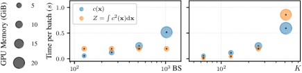
Figure C.1: Evaluating the squared circuit representation adds little overhead during training. By learning by MLE (Eq. 4) and batched gradient descent, the time and space required to compute the partition function of $c^{2}$ (denoted as $Z$) is constant w.r.t. the batch size (BS) (left). By fixing the batch size to 512 and varying the output dimensionality ($K$) of each layer (right), the resources needed to compute $Z$ are similar to the ones needed to evaluate $c$ (denoted as $c(\bm{\mathrm{X}})$). For the left figure, we fix $K=256$ and vary the BS, while for the right figure we fix $\text{BS}=512$ and vary $K$.

Given a tensorized structured-decomposable circuit $c$ defined on a tree RG (Def. 2), Alg. 1 constructs a smooth and decomposable tensorized circuit $c^{2}$. As showed in 1, the complexity of marginalizing $c^{2}$ is linear in the number of layers and quadratic in the complexity of evaluating layers in $c$. However, the MLE objective showed in Eq. 4 suggests we need to compute the partition function $Z=\int c^{2}(\bm{\mathrm{x}})\mathrm{d}\bm{\mathrm{x}}$ only once per parameter update via gradient ascent. This is because $Z$ does not depend on the training data. For this reason, the increased computational burden of evaluating a squared circuit as to compute $Z$ is negligible, and it is independent w.r.t. the batch size. Fig. C.1 illustrates this aspect by comparing the time needed to evaluate $c$ on a batch of data and to compute the partition function $Z$. Below we report the details of this benchmark.

The results showed in Fig. C.1 are obtained by running benchmarks on NPC²s that are similar in size to the ones we experiment with in Sec. 5. That is, we benchmark a mixture of 32 NPC²s, each having an architecture constructed from a randomly-generated tree RG (see Sec. F.3 for details) approximating the density function of BSDS300 (the data set with highest number of variables, see Table F.1). The input layers compute Gaussian distributions.

Appendix D The Signed Log-Sum-Exp Trick

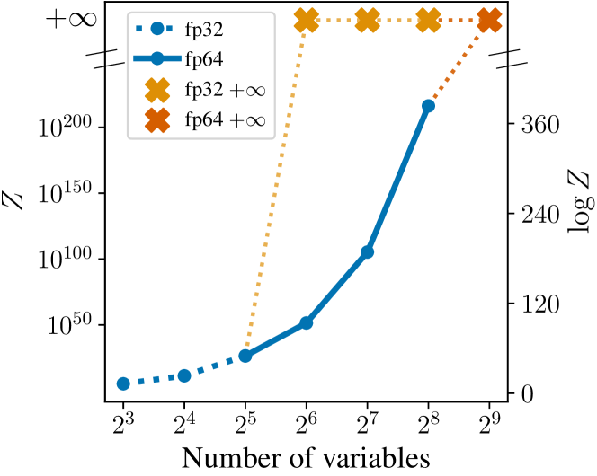
Figure D.1: Squared non-monotonic PCs cannot scale without performing computations in log-space. Partition functions (and their natural logarithm) of squared non-monotonic PCs having Gaussian input units, with increasing number of variables $V$ and having depth $\lceil\log_{2}V\rceil$ computed using 32-bit and 64-bit floating point arithmetic.

Scaling squared non-monotonic PCs to more than a few tens (resp. hundreds) of variables without performing computations in log-space is infeasible in 32-bit (resp. 64-bit) floating point arithmetic, as we illustrate in Fig. D.1. For this reason, we must perform computations in the log-space even in presence of negative values. The idea is to represent non-zero outputs $\bm{\mathrm{y}}\in\mathbb{R}^{S}$ of each layer in terms of the element-wise logarithm of their absolute value $\log|\bm{\mathrm{y}}|$ and their element-wise sign $\operatorname{sign}(\bm{\mathrm{y}})\in\{-1,1\}^{S}$, i.e., such that $\bm{\mathrm{y}}=\operatorname{sign}(\bm{\mathrm{y}})\odot\exp(\log|\bm{\mathrm{y}}|)$.

In practice, we evaluate product and sum layers according to the following evaluation rules. Given an Hadamard product layer $\bm{\mathrm{\ell}}$, then it computes and propagates both $\log|\bm{\mathrm{\ell}}|=\sum_{i=1}^{N}\log|\bm{\mathrm{\ell}}_{i}|$ and $\operatorname{sign}(\bm{\mathrm{\ell}})=\bigodot_{i=1}^{N}\operatorname{sign}(\bm{\mathrm{\ell}}_{i})$ for some inputs $\{\bm{\mathrm{\ell}}_{i}\}_{i=1}^{N}$. Given a sum layer $\bm{\mathrm{\ell}}$ parametrized by $\bm{\mathrm{W}}\in\mathbb{R}^{S\times K}$ and having $\bm{\mathrm{\ell}}^{\prime}$ as input layer, then it computes and propagates both $\log|\bm{\mathrm{\ell}}|=\bm{\mathrm{\alpha}}+\log|\bm{\mathrm{s}}|$ and $\operatorname{sign}(\bm{\mathrm{\ell}})=\operatorname{sign}(\bm{\mathrm{s}})$ where $\bm{\mathrm{\alpha}}$ and $\bm{\mathrm{u}}$ are defined as

$$\bm{\mathrm{\alpha}} =\bm{1}\max\{\log|\bm{\mathrm{\ell}}^{\prime}[j]|\}_{j=1}^{S}$$

$$\bm{\mathrm{s}} =\bm{\mathrm{W}}\left(\operatorname{sign}(\bm{\mathrm{\ell}}^{\prime})\odot\exp(\log|\bm{\mathrm{\ell}}^{\prime}|-\bm{\mathrm{\alpha}})\right)$$

by assuming $\bm{\mathrm{s}}\neq\bm{0}$, $\bm{1}$ denoting a $S$-dimensional vector of ones, $\bm{\mathrm{\ell}}^{\prime}[j]$ denoting the $j$-th entry of the output of $\bm{\mathrm{\ell}}^{\prime}$, and $\exp$ being applied element-wise. We call signed log-sum-exp trick the evaluation rule above for sum layers, which generalizes the log-sum-exp trick (Blanchard et al., 2021) that is used to evaluate tensorized monotonic PC architectures (Peharz et al., 2020a). Finally, note that the evaluation rules above also hold for squared non-monotonic PCs.

For the more general definition of tensorized circuits instead (Def. A.6), given a Kronecker product layer $\bm{\mathrm{\ell}}$, then it computes both $\log|\bm{\mathrm{\ell}}|=\bigoplus_{i=1}^{N}\log|\bm{\mathrm{\ell}}_{i}|$ and $\operatorname{sign}(\bm{\mathrm{\ell}})=\bigotimes_{i=1}^{N}\operatorname{sign}(\bm{\mathrm{\ell}}_{i})$, where $\bigoplus$ denotes an operator similar to the Kronecker product but computing sums instead.

Appendix E Splines as Expressive Input Components

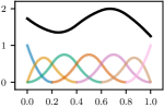
Figure E.1: Splines represent a class of flexible non-linear functions. A quadratic ($k=2$) spline (in black) over $n=4$ knots chosen uniformly in $(0,1)$ (i.e, $0.2$, $0.4$, $0.6$ and $0.8$) is computed by a linear combination of $n+k+1=7$ distinct basis functions (each colored differently).

Polynomials defined on fixed intervals are candidate functions to be modeled by components (resp. input layers) of squared NMMs (Sec. 2) (resp. NPC²s Sec. 3). This is because they can be negative function and their product can be tractably integrated. In particular, we experiment with piecewise polynomials, also called splines. An univariate spline function of order $k$ is a piecewise polynomial defined on a variable $X$, and the $n$ values of $X$ where polynomials meet are called knots. B-splines of order $k$ are basis functions for continuous spline functions of the same degree. In practice, we can represent any spline function $f$ of order $k$ defined over $n$ knots inside an interval $(a,b)$ as a linear combination of $n+k+1$ basis functions, i.e.,

$$f(X)=\sum\nolimits_{i=1}^{n+k+1}\alpha_{i}B_{i,k}(X)$$ (11)

where $\alpha_{i}\in\mathbb{R}$ are the parameters of the spline and $B_{i,k}(X)$ are polynomials of order $k$ (i.e., the basis of $f$), which are unequivocally determined by the choice of the $n$ knots. In particular, each $B_{i,k}(X)$ is a non-negative polynomial that can be recursively defined with the Cox-de-Boor formula (de Boor, 1971; Piegl & Tiller, 1995). Given two splines $f,g$ of order $k$ defined over $n$ knots and represented in terms of $n+k+1$ basis functions as in Eq. 11, we can write the integral of their product as follows.

$$\int_{a}^{b}f(X)g(X)\,\mathrm{d}X=\sum\nolimits_{i=1}^{n+k+1}\sum\nolimits_{j=1}^{n+k+1}\alpha_{i}\beta_{j}\int_{a}^{b}B_{i,k}(X)B_{j,k}(X)\,\mathrm{d}X$$ (12)

where $\alpha_{i}\in\mathbb{R}$ (resp. $\beta_{j}\in\mathbb{R}$) denote the parameters of $f$ (resp. $g$). Therefore, integrating a product of splines requires integrating products of their basis functions. Among the various way of computing Eq. 12 exactly (Vermeulen et al., 1992), we can do it in time $\mathcal{O}(n^{2}\cdot k^{2})$ by representing the product $B_{i,k}(X)B_{j,k}(X)$ as the basis polynomial of another B-spline of order $2k+1$, and finally integrating it in the interval of definition. Fig. E.1 shows an example of a spline.

Since each $B_{i,k}$ is non-negative, we can use B-splines as components (resp. modeled by input layers) of traditional MMs (resp. monotonic PCs) by assuming each spline parameter $\alpha_{i}$ to be non-negative. This is the case of monotonic PCs we experimented with in Sec. 5.

Appendix F Experimental Settings and Complementary Results

F.1 Continuous Synthetic Data

Following (Wenliang et al., 2019) we experiment with monotonic PCs, their squaring and NPC²s on synthetic continuous 2D data sets, named rings, cosine, funnel and banana. We generate each synthetic data set by sampling $10\_000/1\_000/2\_000$ training/validation/test samples. In these experiments, we are interested in studying whether NPC²s can be more expressive in practice, without making assumptions on the data distribution and therefore choosing parametric distributions as components. For this reason, we choose components computing the product of univariate spline functions (App. E) over 32 knots that are uniformly chosen in the data domain. In particular, for monotonic mixtures we restrict the spline coefficients to be non-negative.

Learning and hyperparameters. Since the data is bivariate, the tree on which PCs are defined on consists of just one region that is split in half. All models are learned by batched stochastic gradient descent using the Adam optimizer with default learning rate (Kingma & Ba, 2015) and a batch size of 256. The parameters of all mixtures are initialized by sampling uniformly between 0 and 1. Furthermore, monotonicity in (squared) PCs is endured by exponentiating the parameters.

Fig. 3 shows the density functions estimated from data sets rings and cosine, when using 8 and 12 components, respectively. Moreover, Fig. F.1 report the log-likelihoods and other density functions learned from data sets funnel and banana, when using 4 components.

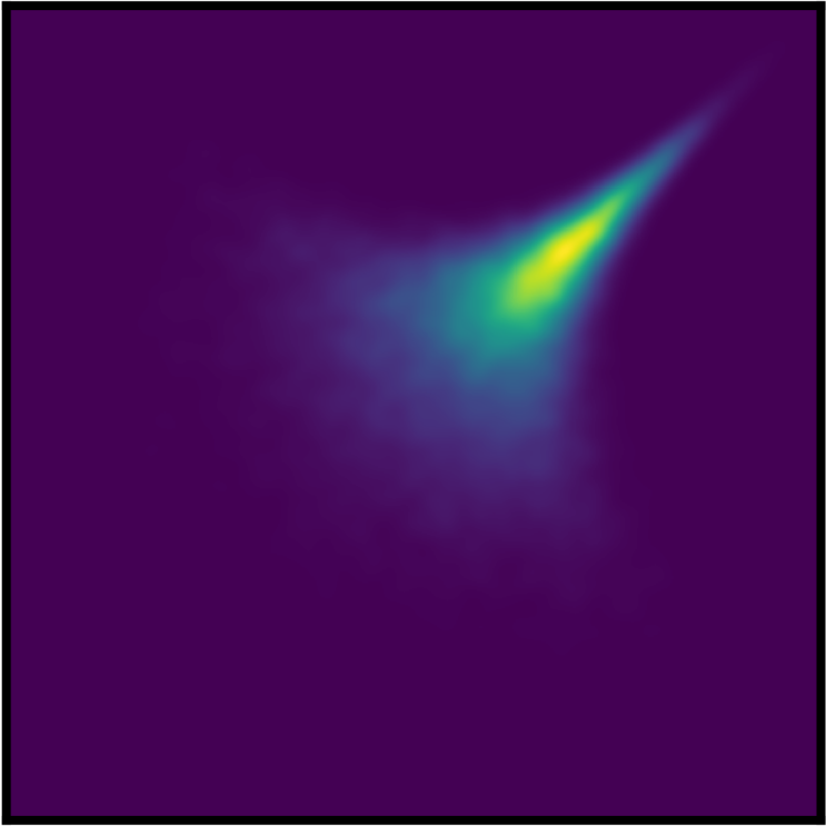
(a) GT

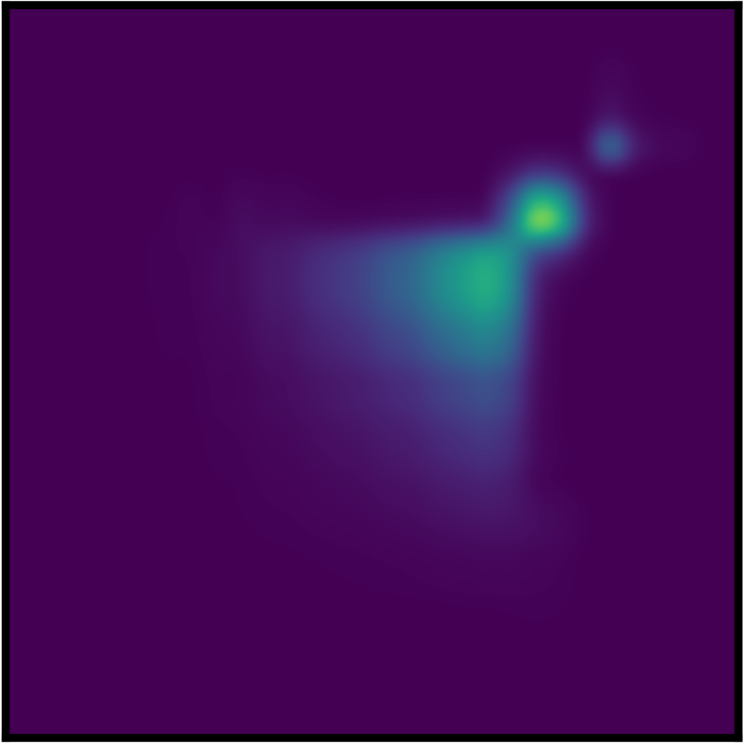
(b) MPC

(c) MPC²

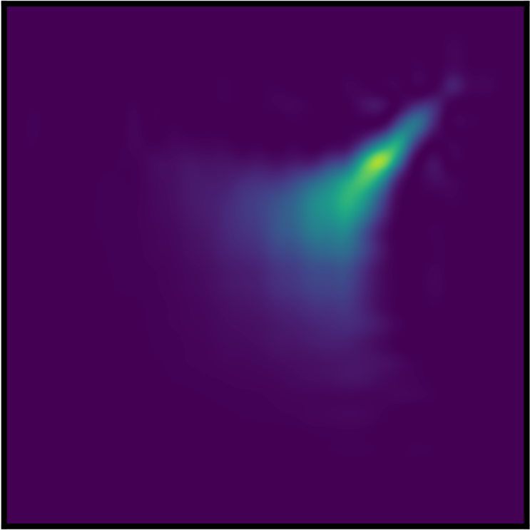
(d) NPC²

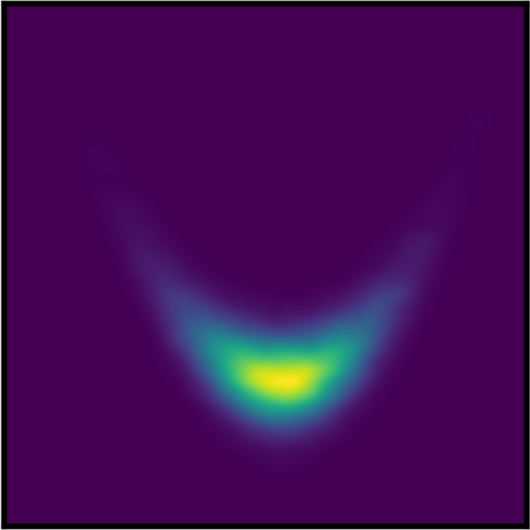
(e) GT

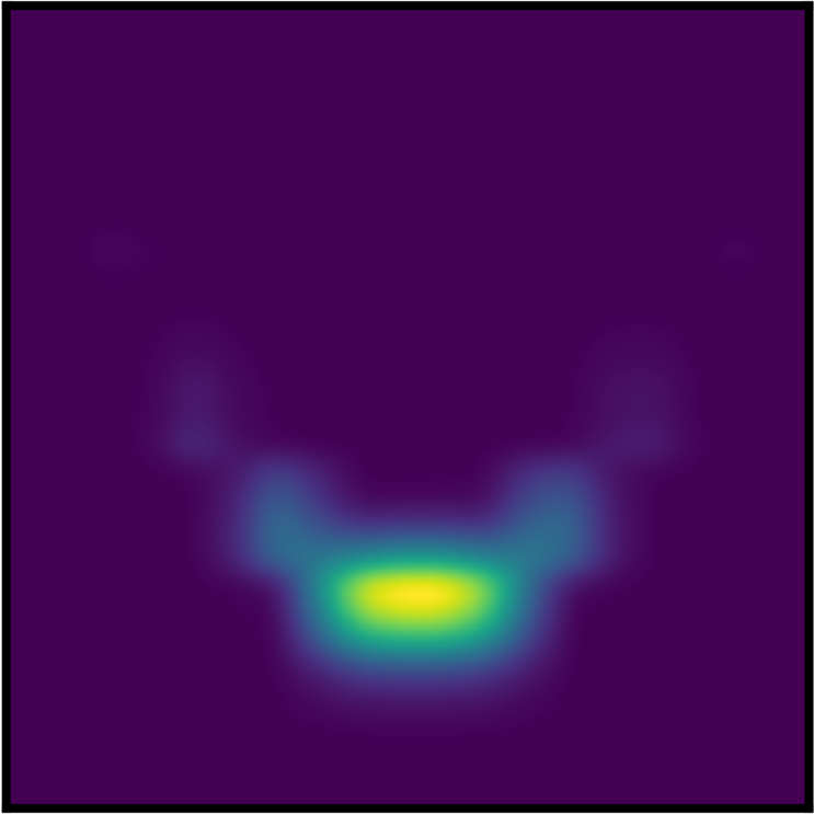
(f) MPC

(g) MPC²

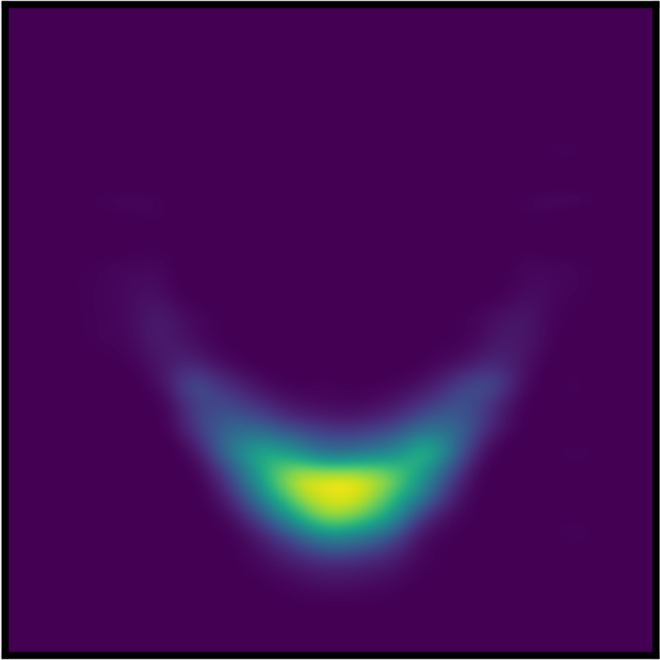
(h) NPC²

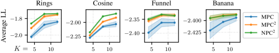
Figure F.1: Negative parameters increases the expressiveness of NPC²s. From left to right (above) and for each bivariate density, we show the ground truth (GT) and its estimation by a monotonic PC (MPC), a squared monotonic PC (MPC²), and a NPC² having input layers computing quadratic splines (App. E) and with the same number of parameters. Moreover, (below) we show the average log-likelihoods (and one standard deviation with 10 independent runs) on unseen data achieved by a monotonic MPC, a squared monotonic MPC², and a NPC² by increasing the dimensionality of input layers $K$.

F.2 Discrete Synthetic Data

For our experiments investigating the flexibility of input layers of NPC²s (Sec. 2) in case of discrete data (Sec. 5), we quantize the bivariate continuous synthetic data sets reported in Sec. F.1. That is, we discretize both continuous variables using $32$ uniform bins each. The resulting target distribution is therefore a probability mass function over two finitely discrete variables.

We experiment with monotonic PCs, their squaring and NPC²s with two families of input layers. First, we investigate very flexible input layers for finitely discrete data: categoricals for monotonic PCs and embeddings for NPC²s. Second, we experiment with the less flexible but more parameter-efficient Binomials. The learning and hyperparameters setting are the same used for the continuous data (see Sec. F.1). Fig. F.2 shows that there is little advantage in subtracting probability mass with respect to monotonic PCs having categorical components. However, in case of the less flexible Binomial components, NPC²s capture the target distribution significantly better. This is also confirmed by the log-likelihoods on unseen data, which we show in Fig. F.2.

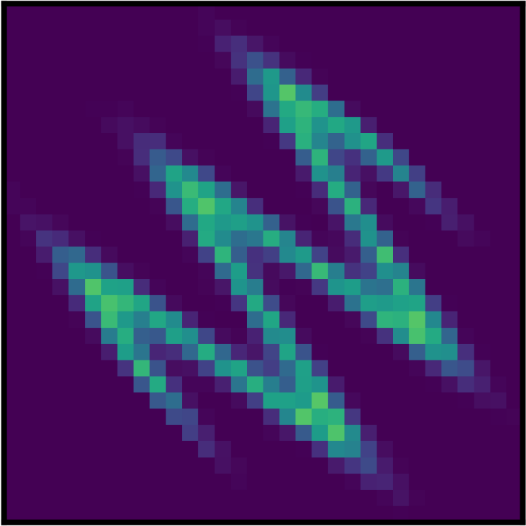
Categorical

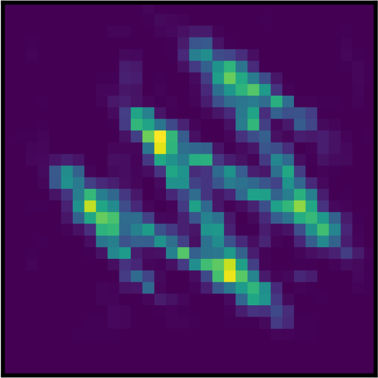
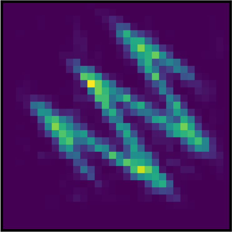
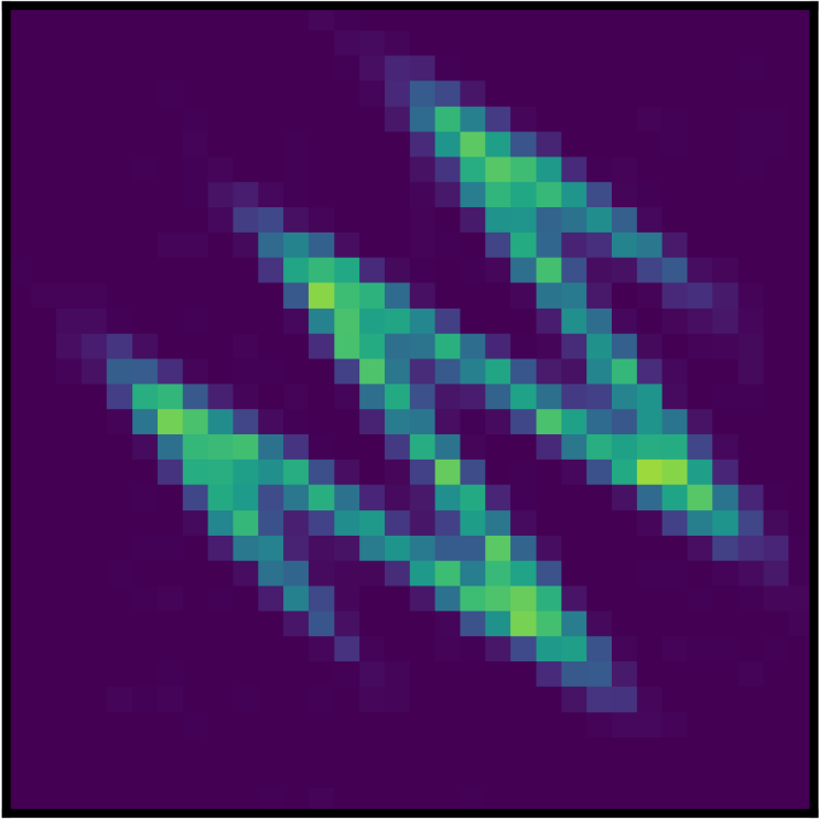
Binomial

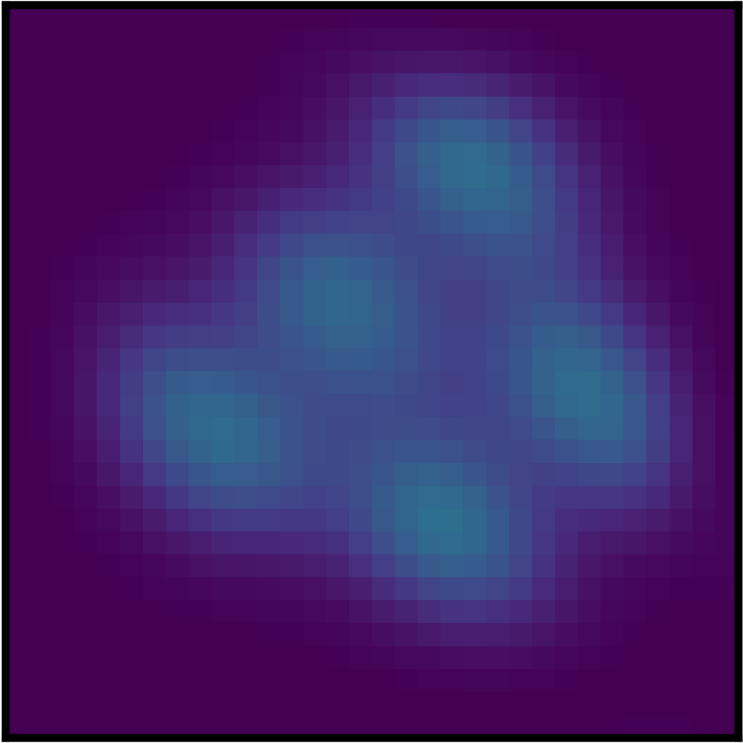
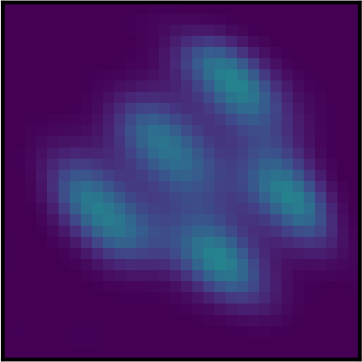
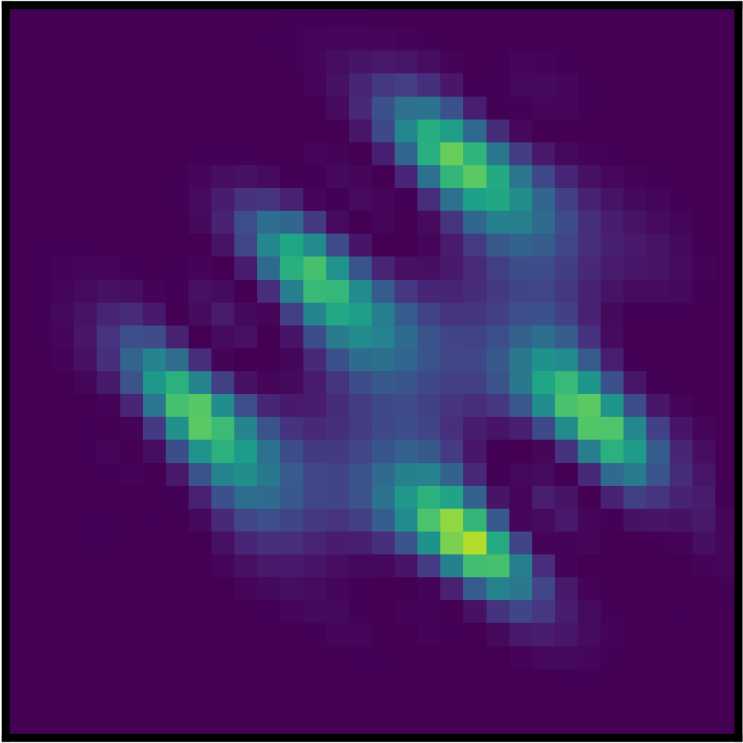
Categorical

Binomial

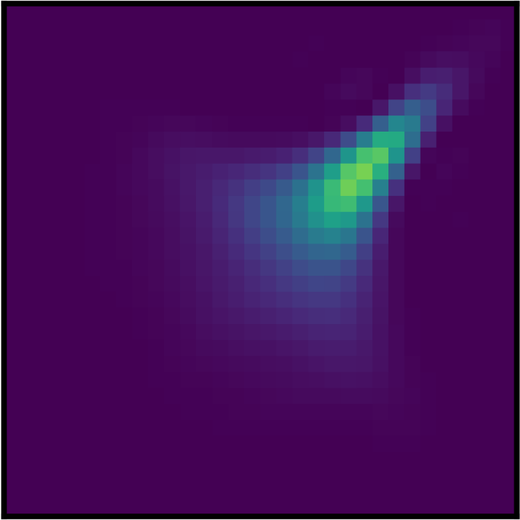
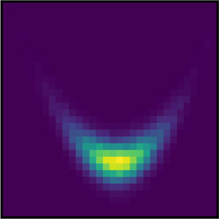
(a) GT

Categorical

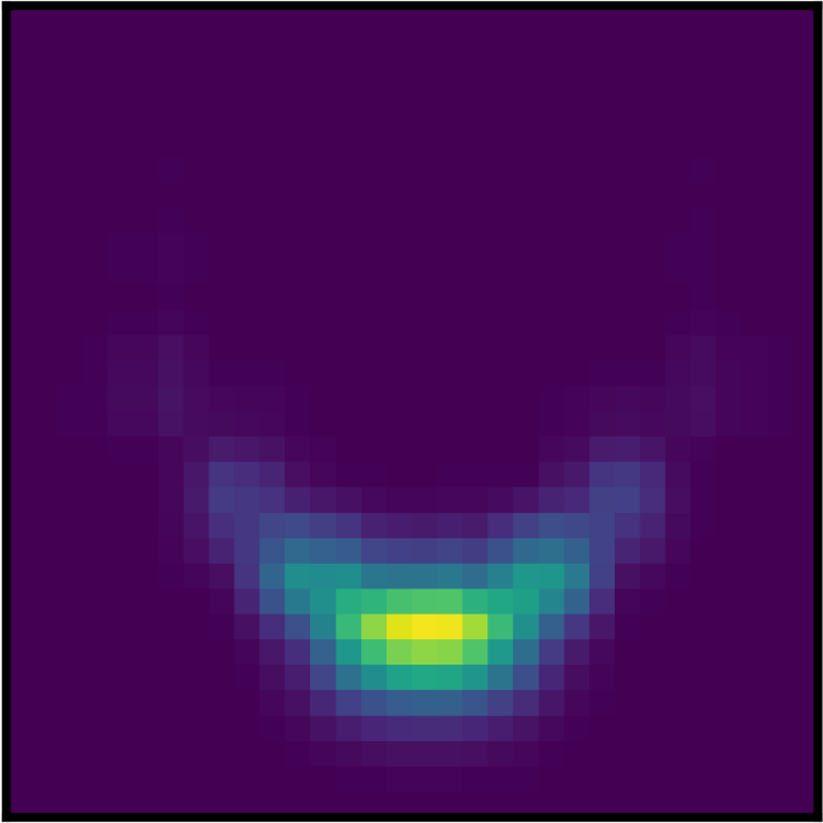
(b) MPC

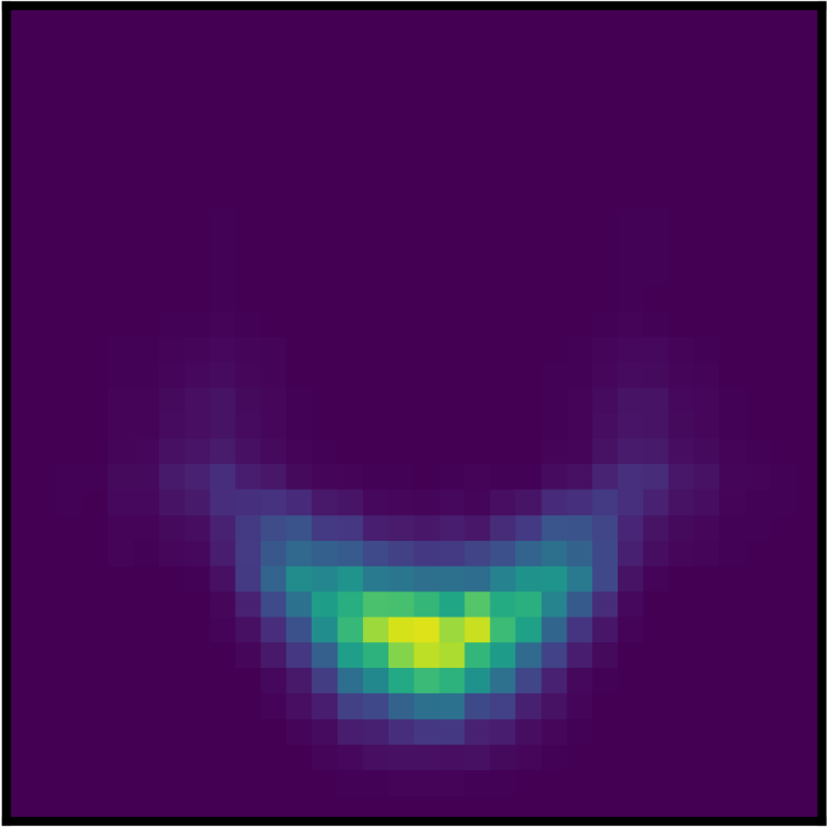
(c) MPC²

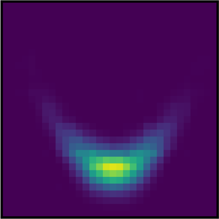
(d) NPC²

Binomial

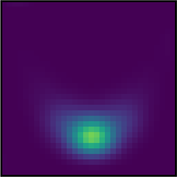
(e) MPC

(f) MPC²

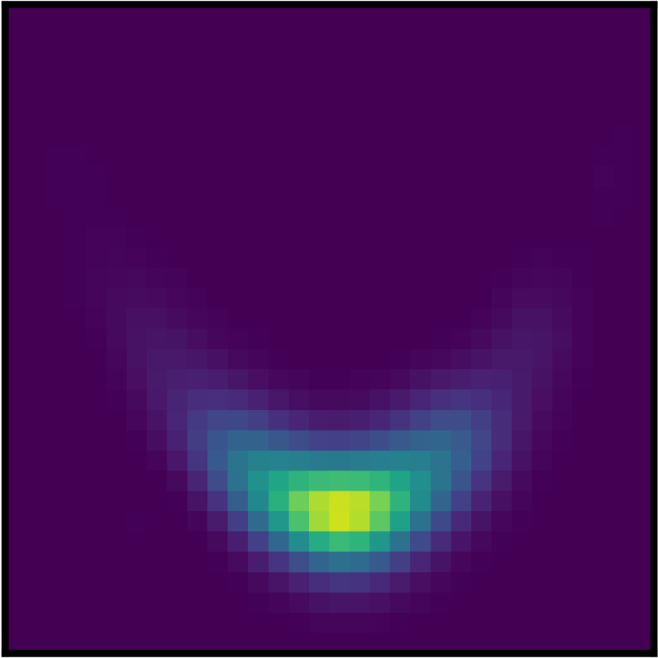
(g) NPC²

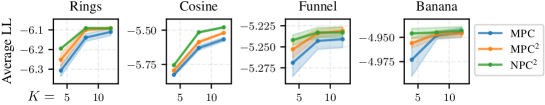
(h) Mixtures with categorical or embedding components.

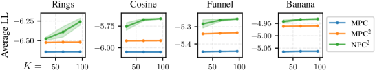
(i) Mixtures with Binomial components.

Figure F.2: Negative parameters increases the expressiveness of NPC²s. From left to right (above) and for each bivariate distribution, we show the ground truth (GT) and its estimation by a monotonic PC (MPC), a squared monotonic PC (MPC²), and a NPC² having input layers computing categoricals (embeddings for NPC²s) and with the same number of parameters. Moreover, we show the average log-likelihoods (and one standard deviation with 10 independent runs) on unseen data achieved by a monotonic MPC, a squared monotonic MPC², and a NPC² with either categorical (a) or Binomial (b) components and by increasing the dimensionality of input layers $K$.

F.3 UCI Continuous Data

Data sets. In Sec. 5 we evaluate NPC²s for density estimation on five multivariate UCI data sets (Dua & Graff, 2017): Power (Hebrail & Berard, 2012), Gas (Fonollosa et al., 2015), Hepmass (Baldi et al., 2016), MiniBooNE (Roe et al., 2004) and BSDS300 patches (Martin et al., 2001) by following the pre-processing by Papamakarios et al. (2017). Table F.1 reports their statistics.

		Number of samples
	$D$	train	validation	test
Power	$6$	$1{,}659{,}917$	$184{,}435$	$204{,}928$
Gas	$8$	$852{,}174$	$94{,}685$	$105{,}206$
Hepmass	$21$	$315{,}123$	$35{,}013$	$174{,}987$
MiniBooNE	$43$	$29{,}556$	$3{,}284$	$3{,}648$
BSDS300	$63$	$1{,}000{,}000$	$50{,}000$	$250{,}000$

Table F.1: UCI data set statistics. Dimensionality $D$ and number of samples of each data set split after the preprocessing by Papamakarios et al. (2017).

Models. We compare monotonic PCs and NPC²s in tensorized form (Def. 1) for density estimation. Since we require structured-decomposability to square circuits (see Sec. 3), we construct their architecture based on tree RGs Def. 2. We choose to experiment with two kinds of tree RGs. Following Peharz et al. (2020b), the first one is tree that is built by recursively partitioning variables evenly and randomly until regions with only one variable are obtained. The second one a linear tree RG that partitions variables one by one, i.e., a set of variables $\{X_{i},\ldots,X_{D}\}$ is partitioned in $\{X_{i}\}$ and $\{X_{i+1},\ldots,X_{D}\}$ for $1\leq i\leq D-1$. The latter RG is the same on which the circuit representation of MPS (and hence TTDE, see Sec. 4) is defined on. More precisely, we replicate random tree RGs (resp. linear tree RGs) eight times by changing the seed (resp. variable ordering). By doing so, our monotonic PCs for these experiments consist of a mixture of tensorized monotonic PCs each defined on a different RG. Conversely, our NPC²s consist of a mixture (with non-negative parameters) of tensorized NPC²s, each constructed by squaring a circuit defined on a different RG. To ensure a fair comparison, monotonic PCs and NPC²s have the exact same structure, but NPC²s allow for negative parameters via the squaring mechanism (see Sec. 3).

Hyperparameters. We search for hyperparameters by running a grid search with both monotonic PCs and NPC²s. For each UCI data set, Tables F.2 and F.3 report the possible value of each hyperparameter, depending on the chosen RG. In case of input layers modeling spline functions (see App. E), we use quadratic splines and select $512$ uniformly in the domain space.

Table F.2: Hyperparameter grid search space for each UCI data set (for BT experiments). Each data set is associated to lists of hyperparameters: learning rate, the dimensionality of layers in tensorized PCs ($K$), batch size, and whether input layers compute Gaussian likelihoods or spline functions (see App. E).

Dataset	Learning rate	$K$	Batch size	Input layer
Power	$[0.01,0.005]$	$[32,\ldots,512]$	$[512,1024,2048]$	[Gaussian, splines]
Gas		$[32,\ldots,1024]$
Hepmass		$[32,\ldots,512]$
MiniBooNE		$[32,\ldots,512]$
BSDS300		$[32,\ldots,256]$

Table F.3: Hyperparameter grid search space for each UCI data set (for LT experiments). Each data set is associated to lists of hyperparameters: learning rate, the dimensionality of layers in tensorized PCs ($K$), batch size, and whether input layers compute Gaussian likelihoods or spline functions (see App. E).

Dataset	Learning rate	$K$	Batch size	Input layer
Power	$[0.005,0.001]$	$[32,\ldots,512]$	$[512,1024,2048]$	[Gaussian, splines]
Gas
Hepmass
MiniBooNE
BSDS300

Figure F.3: Negative parameters make squared non-monotonic PCs more expressive than squared monotonic PCs. NPC²s ($\pm^{2}$, vertical) generally achieve higher log-likelihoods than squared monotonic PCs ($+^{2}$, horizontal) when paired with the same number of units per layer $K$. as shown by the presence of more points in the upper triangle than in the lower triangle for most datasets. Blue circles and red diamonds refer to runs with Gaussian (G) and spline (S) input layers respectively, and darker hues indicate larger $K$. The dashed grey line represents the points of equal log-likelihood for both the NPC² and the squared monotonic PC.

Table F.4: Squared non-monotonic PCs can be more expressive than monotonic PCs. Best average test log-likelihoods and two standard errors achieved by monotonic PCs (MPC) and NPC²s built either from randomized linear tree RGs (LT) or from randomized binary tree RGs (BT) (see Sec. F.3), when compared to baselines. MPC, MPC² and NPC² were experimented with both Gaussian (G) and spline (S) node input layers.

	Power		Gas		Hepmass		MiniBooNE		BSDS300
MADE	-3.08 ±0.03		3.56 ±0.04		-20.98 ±0.02		-15.59 ±0.50		148.85 ±0.28
RealNVP	0.17 ±0.01		8.33 ±0.14		-18.71 ±0.02		-13.84 ±0.52		153.28 ±1.78
MAF	0.24 ±0.01		10.08 ±0.02		-17.73 ±0.02		-12.24 ±0.45		154.93 ±0.28
NSF	0.66 ±0.01		13.09 ±0.02		-14.01 ±0.03		-9.22 ±0.48		157.31 ±0.28
Gaussian	-7.74 ±0.02		-3.58 ±0.75		-27.93 ±0.02		-37.24 ±1.07		96.67 ±0.25
EiNet-LRS	0.36 ±†		4.79 ±†		-22.46 ±†		-34.21 ±†		—
TTDE	0.46 ±†		8.93 ±†		-21.34 ±†		-28.77 ±†		143.30 ±†
	G	S	G	S	G	S	G	S	G	S
MPC (LT)	0.51 ±.01	0.24 ±.01	6.73 ±.03	-2.05 ±.02	-22.07 ±.02	-23.09±.02	-32.48 ±.44	-37.53 ±.46	123.15 ±.28	116.90±.28
MPC2 (LT)	0.49 ±.01	0.39 ±.01	7.06 ±.03	0.95 ±.01	-21.42±.02	-22.24 ±.02	-29.46±.44	-32.81 ±.47	—	—
NPC2 (LT)	0.53 ±.01	0.43 ±.01	9.00 ±.02	3.03 ±.02	-20.66 ±.02	-21.53±.02	-26.68 ±.42	-29.36±.42	112.99 ±.29	120.11±.29
MPC (BT)	0.57 ±.01	0.32 ±.01	5.56 ±.03	-2.55 ±.02	-22.45 ±.02	-24.09 ±.02	-32.11 ±.43	-37.56 ±.46	121.92 ±.29	123.30 ±.29
MPC2 (BT)	0.57 ±.01	0.36 ±.01	8.24 ±.03	0.32 ±.02	-21.47 ±.02	-23.38 ±.02	-29.46 ±.43	-33.43 ±.47	125.56 ±.29	126.85 ±.29
NPC2 (BT)	0.63 ±.01	0.45 ±.01	10.98 ±.02	3.12 ±.01	-20.41±.02	-22.25±.02	-26.92±.44	-30.81±.54	114.47±.28	128.38±.29

Table F.5: Table showing averages and standard deviations of average test set log-likelihoods achieved from running experiments for multiple (N=5) seeds, using the same hyperparameters as were used for achieving results seen in Table F.4.

	Power	Gas	Hepmass	MiniBooNE	BSDS300
MPC (LT)	0.46  ±0.03	7.03  ±0.18	-22.07  ±0.02	-31.79  ±0.39	126.66  ±5.46
MPC (BT)	0.53  ±0.03	6.16  ±0.56	-22.42  ±0.45	-33.30  ±0.98	122.77  ±0.71
NPC2 (LT)	0.42  ±0.11	8.97  ±0.08	-20.67  ±0.05	-29.58  ±0.29	127.58  ±4.66
NPC2 (BT)	0.62  ±0.01	10.55  ±0.39	-20.48  ±0.11	-27.64  ±0.44	128.45  ±0.52

Table F.6: Table showing the hyperparameter combinations found via a grid search, which were used for achieving results seen in Table F.4.

Model	Data set	$K$	Batch size	learning-rate	Input layer
MPC (BT)	Power	512	512	0.01	G
	Gas	1024	4096	0.01	G
	Hepmass	128	512	0.01	G
	MiniBooNE	32	512	0.01	G
	BSDS300	512	512	0.01	S
MPC (LT)	Power	512	512	0.001	G
	Gas	512	1024	0.001	G
	Hepmass	512	512	0.005	G
	MiniBooNE	512	1024	0.005	G
	BSDS300	64	512	0.005	S
NPC2 (BT)	Power	512	512	0.01	G
	Gas	1024	512	0.01	G
	Hepmass	256	512	0.01	G
	MiniBooNE	32	512	0.01	G
	BSDS300	128	512	0.01	S
NPC2 (LT)	Power	512	512	0.001	G
	Gas	512	512	0.001	G
	Hepmass	256	512	0.001	G
	MiniBooNE	128	2048	0.005	G
	BSDS300	32	1024	0.001	S

F.4 Large Language Model Distillation

Data set. Given $p^{*}(\bm{\mathrm{x}})$ the distribution modeled by GPT2 over sentences $\bm{\mathrm{x}}=[x_{1},\ldots,x_{D}]$ having maximum length $D$, we aim to minimize the Kullback-Leibler divergence $\mathrm{KL}[p^{*}\mid p]$, where $p$ is modeled by a PC. Minimizing such divergence is equivalent to learn the PC by maximum-likelihood on data sampled by GPT2. Therefore, following the experimental setting by Zhang et al. (2023) we sample a data set of 4M sentences using GPT2 having bounded length $D=32$, i.e., with a maximum of $D=32$ tokens.

Models. Then, we learn a monotonic PC and a NPC² as tensorized circuits whose architecture is determined by a linear tree RG (Def. 2), i.e., a region graph that recursively partitions each set of finitely-discrete variables $\{X_{i},\ldots,X_{D}\}$ into $\{X_{i}\}$ and $\{X_{i+1},\ldots,X_{D}\}$ for $1\leq i\leq D-1$ (e.g., see Fig. 2). This is because we are interested in exploiting the sequential dependencies between words in a sentence. By enforcing monotonicity, we recover that the monotonic PC is equivalent to an inhomogenous hidden Markov model (HMM), and that that NPC² corresponds to a Born machine (see Sec. B.4.1 for details).

Hyperparameters. All PCs are learned by batched stochastic gradient descent using (Kingma & Ba, 2015) as optimizer using batch size $4096$. We perform multiple runs by exploring combinations of learning rates and initialization. For monotonic PCs, we run experiments by choosing learning rates in $\{5\cdot 10^{-3},10^{-2},5\cdot 10^{-2}\}$ and initializing parameters by sampling uniformly in $(0,1)$, by sampling from a standard log-normal distribution, and from a Dirichlet distribution with concentration values set to $1$. Similarly for NPC²s, we run experiments by choosing the same learning rates for monotonic PCs, but using different initialization. In addition to sampling uniformly in $(0,1)$, we also initialize the parameters by sampling from a standard normal distribution. By doing so, we initialize an approximately even number of positive and negative parameters. Moreover, we also initialize parameters by sampling from a normal distribution with mean $1$ and standard deviation $1$, which initializes more parameters to be positive.

References

- Ahmed et al. (2022) Kareem Ahmed, Stefano Teso, Kai-Wei Chang, Guy Van den Broeck, and Antonio Vergari. Semantic probabilistic layers for neuro-symbolic learning. In Advances in Neural Information Processing Systems 35 (NeurIPS), volume 35, pp. 29944–29959. Curran Associates, Inc., 2022.
- Baldi et al. (2016) Pierre Baldi, Kyle Cranmer, Taylor Faucett, Peter Sadowski, and Daniel Whiteson. Parameterized neural networks for high-energy physics. European Physical Journal C, 76(5):235, 2016. doi: 10.1140/epjc/s10052-016-4099-4.
- Blanchard et al. (2021) Pierre Blanchard, Desmond J. Higham, and Nicholas J. Higham. Accurately computing the log-sum-exp and softmax functions. Institute of Mathematics and its Applications Journal of Numerical Analysis (IMAJNA), 41(4):2311–2330, 2021.
- Cheng et al. (2019) Song Cheng, Lei Wang, Tao Xiang, and Pan Zhang. Tree tensor networks for generative modeling. Physical Review B, 99(15):155131, 2019.
- Choi et al. (2015) Arthur Choi, Guy Van den Broeck, Adnan Darwiche, Qiang Yang, and Michael Wooldridge. Tractable learning for structured probability spaces: A case study in learning preference distributions. In 24th International Joint Conference on Artificial Intelligence (IJCAI), volume 2015, pp. 2861–2868. IJCAI, 2015.
- Choi et al. (2020) YooJung Choi, Antonio Vergari, and Guy Van den Broeck. Probabilistic circuits: A unifying framework for tractable probabilistic modeling. Technical report, University of California, Los Angeles (UCLA), 2020.
- Dang et al. (2021) Meihua Dang, Antonio Vergari, and Guy Van den Broeck. Strudel: A fast and accurate learner of structured-decomposable probabilistic circuits. The International Journal of Approximate Reasoning (IJAR), 140:92–115, 2021.
- Darwiche (2001) Adnan Darwiche. Decomposable negation normal form. Journal of the ACM (JACM), 48:608–647, 2001.
- Darwiche (2009) Adnan Darwiche. Modeling and Reasoning with Bayesian Networks. Cambridge University Press, 2009.
- Darwiche & Marquis (2002) Adnan Darwiche and Pierre Marquis. A knowledge compilation map. Journal of Artificial Intelligence Research (JAIR), 17:229–264, 2002.
- Daubechies (1992) Ingrid Daubechies. Ten lectures on wavelets. Computers in Physics, 6:697–697, 1992.
- de Boor (1971) Carl de Boor. Subroutine package for calculating with B-splines. Technical report, Los Alamos National Lab. (LANL), 1971.
- de Colnet & Mengel (2021) Alexis de Colnet and Stefan Mengel. A compilation of succinctness results for arithmetic circuits. In 18th International Conference on Principles of Knowledge Representation and Reasoning (KR), pp. 205–215, 2021.
- De Wolf (2003) Ronald De Wolf. Nondeterministic quantum query and communication complexities. SIAM Journal on Computing, 32(3):681–699, 2003.
- Dennis (2016) Aaron W. Dennis. Algorithms for Learning the Structure of Monotone and Nonmonotone Sum-Product Networks. PhD thesis, Brigham Young University, 2016.
- Dennis & Ventura (2012) Aaron W. Dennis and Dan Ventura. Learning the architecture of sum-product networks using clustering on variables. In Advances in Neural Information Processing Systems 25 (NeurIPS), pp. 2033–2041. Curran Associates, Inc., 2012.
- Di Mauro et al. (2017) Nicola Di Mauro, Antonio Vergari, Teresa M. A. Basile, and Floriana Esposito. Fast and accurate density estimation with extremely randomized cutset networks. In Machine Learning and Knowledge Discovery in Databases: ECML PKDD, pp. 203–219. Springer, 2017.
- Di Mauro et al. (2021) Nicola Di Mauro, Gennaro Gala, Marco Iannotta, and Teresa Maria Altomare Basile. Random probabilistic circuits. In 37th Conference on Uncertainty in Artificial Intelligence (UAI), volume 161, pp. 1682–1691. PMLR, 2021.
- Dinh et al. (2017) Laurent Dinh, Jascha Sohl-Dickstein, and Samy Bengio. Density estimation using Real NVP. In 5th International Conference on Learning Representations (ICLR), 2017.
- Dirac (1930) Paul Adrien Maurice Dirac. The Principles of Quantum Mechanics. Clarendon Press, Oxford,, 1930.
- Dua & Graff (2017) Dheeru Dua and Casey Graff. UCI Machine Learning Repository, 2017.
- Durkan et al. (2019) Conor Durkan, Artur Bekasov, Iain Murray, and George Papamakarios. Neural spline flows. In Advances in Neural Information Processing Systems 32 (NeurIPS), pp. 7511–7522. Curran Associates, Inc., 2019.
- Fiorini et al. (2015) Samuel Fiorini, Serge Massar, Sebastian Pokutta, Hans Raj Tiwary, and Ronald De Wolf. Exponential lower bounds for polytopes in combinatorial optimization. Journal of the ACM (JACM), 62(2):1–23, 2015.
- Fonollosa et al. (2015) Jordi Fonollosa, Sadique Sheik, Ramón Huerta, and Santiago Marco. Reservoir computing compensates slow response of chemosensor arrays exposed to fast varying gas concentrations in continuous monitoring. Sensors and Actuators B: Chemical, 215:618–629, 2015.
- Germain et al. (2015) Mathieu Germain, Karol Gregor, Iain Murray, and Hugo Larochelle. MADE: Masked autoencoder for distribution estimation. In 32nd International Conference on Machine Learning (ICML), pp. 881 – 889, 2015.
- Gillis (2020) Nicolas Gillis. Nonnegative Matrix Factorization. Society for Industrial and Applied Mathematics (SIAM), 2020.
- Glasser et al. (2019) Ivan Glasser, Ryan Sweke, Nicola Pancotti, Jens Eisert, and Ignacio Cirac. Expressive power of tensor-network factorizations for probabilistic modeling. In Advances in Neural Information Processing Systems 32 (NeurIPS), pp. 1498–1510. Curran Associates, Inc., 2019.
- Han et al. (2018) Zhao-Yu Han, Jun Wang, Heng Fan, Lei Wang, and Pan Zhang. Unsupervised generative modeling using matrix product states. Physical Review X, 8:031012, Jul 2018.
- Hebrail & Berard (2012) Georges Hebrail and Alice Berard. Individual household electric power consumption. UCI Machine Learning Repository, 2012.
- Hinton (2002) Geoffrey E. Hinton. Training products of experts by minimizing contrastive divergence. Neural Computation, 14:1771–1800, 2002.
- Hong & Gao (2021) Xia Hong and Junbin Gao. Estimating the square root of probability density function on Riemannian manifold. Expert Systems - The Journal of Knowledge Engineering, 38(7), 2021.
- Hoory et al. (2006) Shlomo Hoory, Nathan Linial, and Avi Wigderson. Expander graphs and their applications. Bulletin of the American Mathematical Society, 43(4):439–561, 2006.
- Huggins et al. (2018) William J. Huggins, Piyush S. Patil, Bradley K. Mitchell, K. Birgitta Whaley, and Edwin Miles Stoudenmire. Towards quantum machine learning with tensor networks. Quantum Science and Technology, 4, 2018.
- Jiang et al. (1999) Renyan Jiang, Ming J. Zuo, and Han-Xiong Li. Weibull and inverse weibull mixture models allowing negative weights. Reliability Engineering & System Safety, 66(3):227–234, 1999.
- Kingma & Ba (2015) Diederik P. Kingma and Jimmy Ba. Adam: A method for stochastic optimization. In 3rd International Conference on Learning Representations (ICLR), 2015.
- Kolda & Bader (2009) Tamara G. Kolda and Brett W. Bader. Tensor decompositions and applications. Society of Industrial and Applied Mathematics (SIAM) Review, 51(3):455–500, 2009.
- LeCun et al. (2006) Yann LeCun, Sumit Chopra, Raia Hadsell, Marc’Aurelio Ranzato, and Fujie Huang. A tutorial on energy-based learning. Predicting Structured Data, 2006.
- Liu & Van den Broeck (2021) Anji Liu and Guy Van den Broeck. Tractable regularization of probabilistic circuits. In Advances in Neural Information Processing Systems 34 (NeurIPS), pp. 3558–3570. Curran Associates, Inc., 2021.
- Liu et al. (2023) Anji Liu, Honghua Zhang, and Guy Van den Broeck. Scaling up probabilistic circuits by latent variable distillation. In 11th International Conference on Learning Representations (ICLR), 2023.
- Liu & Wang (2018) Jin-Guo Liu and Lei Wang. Differentiable learning of quantum circuit born machines. Physical Review A, 98(6):062324, 2018.
- Loconte et al. (2023) Lorenzo Loconte, Nicola Di Mauro, Robert Peharz, and Antonio Vergari. How to turn your knowledge graph embeddings into generative models via probabilistic circuits. In Advances in Neural Information Processing Systems 37 (NeurIPS). Curran Associates, Inc., 2023.
- Mari et al. (2023) Antonio Mari, Gennaro Vessio, and Antonio Vergari. Unifying and understanding overparameterized circuit representations via low-rank tensor decompositions. In 6th Workshop on Tractable Probabilistic Modeling, 2023.
- Marteau-Ferey et al. (2020) Ulysse Marteau-Ferey, Francis Bach, and Alessandro Rudi. Non-parametric models for non-negative functions. In Advances in Neural Information Processing Systems 33 (NeurIPS), pp. 12816–12826, 2020.
- Martens & Medabalimi (2014) James Martens and Venkatesh Medabalimi. On the expressive efficiency of sum product networks. arXiv preprint arXiv:1411.7717, 2014.
- Martin et al. (2001) David Martin, Charless Fowlkes, Doron Tal, and Jitendra Malik. A database of human segmented natural images and its application to evaluating segmentation algorithms and measuring ecological statistics. In 8th International Conference on Computer Vision (ICCV), volume 2, pp. 416–423. IEEE, 2001.
- McLachlan et al. (2019) Geoffrey J. McLachlan, Sharon X. Lee, and Suren I. Rathnayake. Finite mixture models. Annual Review of Statistics and its Application, 6:355–378, 2019.
- Nguyen et al. (2019) TrungTin Nguyen, Hien Duy Nguyen, Faicel Chamroukhi, and Geoffrey J. McLachlan. Approximation by finite mixtures of continuous density functions that vanish at infinity. Cogent Mathematics & Statistics, 7, 2019.
- Novikov et al. (2021) Georgii S. Novikov, Maxim E. Panov, and Ivan V. Oseledets. Tensor-train density estimation. In 37th Conference on Uncertainty in Artificial Intelligence (UAI), volume 161 of Proceedings of Machine Learning Research, pp. 1321–1331. PMLR, 2021.
- Orús (2013) Román Orús. A practical introduction to tensor networks: Matrix product states and projected entangled pair states. Annals of Physics, 349:117–158, 2013.
- Papamakarios et al. (2017) George Papamakarios, Theo Pavlakou, and Iain Murray. Masked autoregressive flow for density estimation. In Advances in Neural Information Processing Systems 30 (NeurIPS), pp. 2338–2347. Curran Associates, Inc., 2017.
- Papamakarios et al. (2021) George Papamakarios, Eric Nalisnick, Danilo Jimenez Rezende, Shakir Mohamed, and Balaji Lakshminarayanan. Normalizing flows for probabilistic modeling and inference. The Journal of Machine Learning Research (JMLR), 22(1):2617–2680, 2021.
- Peharz et al. (2017) Robert Peharz, Robert Gens, Franz Pernkopf, and Pedro M. Domingos. On the latent variable interpretation in sum-product networks. IEEE Transactions on Pattern Analalysis and Machine Intelligence, 39(10):2030–2044, 2017.
- Peharz et al. (2020a) Robert Peharz, Steven Lang, Antonio Vergari, Karl Stelzner, Alejandro Molina, Martin Trapp, Guy Van Den Broeck, Kristian Kersting, and Zoubin Ghahramani. Einsum networks: Fast and scalable learning of tractable probabilistic circuits. In 37th International Conference on Machine Learning (ICML), volume 119 of Proceedings of Machine Learning Research, pp. 7563–7574. PMLR, 2020a.
- Peharz et al. (2020b) Robert Peharz, Antonio Vergari, Karl Stelzner, Alejandro Molina, Xiaoting Shao, Martin Trapp, Kristian Kersting, and Zoubin Ghahramani. Random sum-product networks: A simple and effective approach to probabilistic deep learning. In 35th Conference on Uncertainty in Artificial Intelligence (UAI), volume 115 of Proceedings of Machine Learning Research, pp. 334–344. PMLR, 2020b.
- Pérez-García et al. (2007) David Pérez-García, F. Verstraete, Michael M. Wolf, and Juan Ignacio Cirac. Matrix product state representations. Quantum Information and Computing, 7(5):401–430, 2007. ISSN 1533-7146.
- Piegl & Tiller (1995) Les A. Piegl and Wayne Tiller. The NURBS book. In Monographs in Visual Communication, 1995.
- Pinheiro & Vidakovic (1997) Aluisio Pinheiro and Brani Vidakovic. Estimating the square root of a density via compactly supported wavelets. Computational Statistics and Data Analysis, 25(4):399–415, 1997.
- Pipatsrisawat & Darwiche (2008) Knot Pipatsrisawat and Adnan Darwiche. New compilation languages based on structured decomposability. In 23rd Conference on Artificial Intelligence (AAAI), volume 8, pp. 517–522, 2008.
- Poon & Domingos (2011) Hoifung Poon and Pedro Domingos. Sum-product networks: A new deep architecture. In IEEE International Conference on Computer Vision Workshops (ICCV Workshops), pp. 689–690. IEEE, 2011.
- Rabusseau & Denis (2014) Guillaume Rabusseau and François Denis. Learning negative mixture models by tensor decompositions. arXiv preprint arXiv:1403.4224, 2014.
- Rasmussen & Williams (2005) Carl Edward Rasmussen and Christopher K. I. Williams. Gaussian Processes for Machine Learning. Adaptive Computation and Machine Learning. MIT Press, 2005.
- Roe et al. (2004) Byron P. Roe, Hai-Jun Yang, Ji Zhu, Yong Liu, Ion Stancu, and Gordon McGregor. Boosted decision trees as an alternative to artificial neural networks for particle identification. Nuclear Instruments & Methods in Physics Research Section A-accelerators Spectrometers Detectors and Associated Equipment, 543:577–584, 2004.
- Roughgarden (2016) Tim Roughgarden. Communication complexity (for algorithm designers). Foundations and Trends® in Theoretical Computer Science, 11(3–4):217–404, 2016.
- Rudi & Ciliberto (2021) Alessandro Rudi and Carlo Ciliberto. PSD representations for effective probability models. In Advances in Neural Information Processing Systems 34 (NeurIPS), pp. 19411–19422. Curran Associates, Inc., 2021.
- Schölkopf & Smola (2001) Bernhard Schölkopf and Alex Smola. Learning with kernels: support vector machines, regularization, optimization, and beyond. In Adaptive Computation and Machine Learning Series. MIT Press, 2001.
- Schollwoeck (2010) Ulrich Schollwoeck. The density-matrix renormalization group in the age of matrix product states. Annals of Physics, 326:96–192, 2010.
- Seeger (2005) Matthias Seeger. Expectation propagation for exponential families. Technical report, Department of EECS, University of California at Berkeley, 2005.
- Shen et al. (2016) Yujia Shen, Arthur Choi, and Adnan Darwiche. Tractable operations for arithmetic circuits of probabilistic models. In Advances in Neural Information Processing Systems 29 (NeurIPS). Curran Associates, Inc., 2016.
- Shih & Ermon (2020) Andy Shih and Stefano Ermon. Probabilistic circuits for variational inference in discrete graphical models. In Advances in Neural Information Processing Systems 33 (NeurIPS). Curran Associates, Inc., 2020.
- Shpilka & Yehudayoff (2010) Amir Shpilka and Amir Yehudayoff. Arithmetic circuits: A survey of recent results and open questions. Founddations and Trends in Theoretical Computer Science, 5:207–388, 2010.
- Sidheekh et al. (2023) Sahil Sidheekh, Kristian Kersting, and Sriraam Natarajan. Probabilistic flow circuits: Towards unified deep models for tractable probabilistic inference. In 39th Conference on Uncertainty in Artificial Intelligence (UAI), volume 216 of Proceedings of Machine Learning Research, pp. 1964–1973. PMLR, 2023.
- Stoudenmire & Schwab (2016) Edwin Stoudenmire and David J Schwab. Supervised learning with tensor networks. In Advances in Neural Information Processing Systems 29 (NeurIPS), pp. 4799–4807. Curran Associates, Inc., 2016.
- Tsuchida et al. (2023) Russell Tsuchida, Cheng Soon Ong, and Dino Sejdinovic. Squared neural families: A new class of tractable density models. arXiv preprint arXiv:2305.13552, 2023.
- Valiant (1979) Leslie G. Valiant. Negation can be exponentially powerful. In 11th Annual ACM Symposium on Theory of Computing, pp. 189–196, 1979.
- Vergari et al. (2019a) Antonio Vergari, Nicola Di Mauro, and Floriana Esposito. Visualizing and understanding sum-product networks. Machine Learning, 108(4):551–573, 2019a.
- Vergari et al. (2019b) Antonio Vergari, Nicola Di Mauro, and Guy Van den Broeck. Tractable probabilistic models: Representations, algorithms, learning, and applications. Tutorial at the 35th Conference on Uncertainty in Artificial Intelligence (UAI), 2019b.
- Vergari et al. (2021) Antonio Vergari, YooJung Choi, Anji Liu, Stefano Teso, and Guy Van den Broeck. A compositional atlas of tractable circuit operations for probabilistic inference. In Advances in Neural Information Processing Systems 34 (NeurIPS), pp. 13189–13201. Curran Associates, Inc., 2021.
- Vermeulen et al. (1992) Allan H. Vermeulen, Richard H. Bartels, and Glenn R. Heppler. Integrating products of B-splines. SIAM Journal on Scientific and Statistical Computing, 13:1025–1038, 1992.
- Wang et al. (2022) Benjie Wang, Matthew R. Wicker, and Marta Kwiatkowska. Tractable uncertainty for structure learning. In 39th International Conference on Machine Learning (ICML), pp. 23131–23150. PMLR, 2022.
- Wenliang et al. (2019) Li Wenliang, Danica J. Sutherland, Heiko Strathmann, and Arthur Gretton. Learning deep kernels for exponential family densities. In 36th International Conference on Machine Learning (ICML), volume 97 of Proceedings of Machine Learning Research, pp. 6737–6746. PMLR, 2019.
- Zhang & Zhang (2005) Baibo Zhang and Changshui Zhang. Finite mixture models with negative components. In 4th International Conference on Machine Learning and Data Mining in Pattern Recognition (MLDM), pp. 31–41. Springer, 2005.
- Zhang et al. (2021) Honghua Zhang, Brendan Juba, and Guy Van den Broeck. Probabilistic generating circuits. In International Conference on Machine Learning, pp. 12447–12457. PMLR, 2021.
- Zhang et al. (2023) Honghua Zhang, Meihua Dang, Nanyun Peng, and Guy Van den Broeck. Tractable control for autoregressive language generation. In 40th International Conference on Machine Learning (ICML), volume 202 of Proceedings of Machine Learning Research, pp. 40932–40945. PMLR, 2023.