Exact Entanglement Propagation Dynamics in Integrable Heisenberg Chains

Abstract

The exact single-magnon entanglement evolution in Heisenberg chains is obtained using the Quantum Correlation Transfer Function (QCTF) formulation. The individual spins’ entanglement is given by a hypergeometric function, and its transient behavior is described via a Bessel function of the first kind. The presented characterization through the lens of QCTF allowed for calculating the ballistic single-magnon entanglement edge velocity in Heisenberg chains, which has not been achieved before. Our results can be extended to the multi-magnon regime, therefore opening up the means to explain equilibration dynamics and thermodynamics in Heisenberg chains.

Introduction.- Understanding entanglement propagation in non-equilibrium many-body quantum systems is valuable for both fundamental and practical reasons, especially given new developments in the understanding of the interrelation between entanglement and thermodynamics in quantum systems [1, 2, 3, 4]. Integrable quantum systems have been a primary subject in the study of entanglement dynamics due to their importance and algebraic structure [5]. In this class of quantum systems, quasi-particles can transport correlations throughout the many-body lattice [6, 7, 8, 9, 10, 11, 12]. The development of macroscopic theories, including Generalized Hydrodynamics (GHD) [13], to study finite-temperature quasi-particle transport has been an extensive, ongoing research effort [14, 15, 16, 17]. In isolated quantum systems, thermal behavior re-emerges through entanglement between the constituents [18, 19, 20, 21]. In this case, the long-time behavior of generic local observables is conjectured to be given by conventional thermodynamics ensembles at relevant effective temperatures [22, 23, 24, 25, 26]. In the case of integrable systems, Generalized Gibbs Ensembles have been used extensively to predict the asymptotic behavior of observables [27, 28, 29, 30, 31], including both successful [32, 33, 34, 35] and unsuccessful [36, 37] cases of this formulation in studying the Heisenberg model. Despite the analytical progress in studying entanglement, except in rare cases [38, 39, 40], the exact time dependence, in particular the transient behavior, and the underlying mechanism of the equilibration process thus far have remained confined to numerical treatments.

In relativistic quantum systems with short-length interactions, Lieb and Robinson’s theorem provides a bound based on the maximum group velocity and a resulting causality light-cone for the ballistic propagation of correlations, beyond which correlations must decay exponentially [41, 42]. This phenomenon has been experimentally observed in several instances [43, 44]. The presence of long-range interactions breaks the Lieb-Robinson bound, but further modifications can be made to obtain the correlation transport velocity [45, 46, 47, 48, 49], which has proven to remain finite under certain circumstances [50]. Moreover, the spread of correlations is shown to have a double causality structure with different velocities, where one case corresponds to the edge - which is faster, given by the phase velocity in the lattice - and the other case is associated with the extremum of correlation transport [47, 51].

This paper presents analytical results on entanglement propagation in integrable Heisenberg chains through a new lens, the Quantum Correlation Transfer Functions (QCTFs) [52, 53]. In this framework, the dynamical properties of a subsystem’s entanglement are encoded in the residues of a complex (QCTF) function which can be calculated directly from the system’s Hamiltonian and its pre-quench state. Hence, in this framework, exponentially expensive (i.e., with respect to the number of bodies in the system) calculations of the system’s time evolution can be avoided and the evolution of entanglement can be directly obtained from the system’s Hamiltonian. To this end, the dynamics of entanglement is quantified using a geometric measure: the squared area spanned by projected wave functions (onto a local basis for the subsystem of interest) [52]. In the case of two-energy level subsystems, this measure of entanglement reduces to the determinant of the reduced density matrices in the Laplace domain. In order to obtain the QCTF function, we assign a unique integer number to an arbitrary set of eigenstates for the underlying Hilbert space; nevertheless, the residues of the QCTF, encoding entanglement between subsystems, are invariant to the chosen basis.

This treatment enables a full analysis of the single-magnon entanglement quench dynamics in ferromagnetic Heisenberg spin-$\frac{1}{2}$ chains with arbitrary length, thereby going beyond numerical analyses, mean-field models, and tensor-network-based approaches. The choice of local quench based on a single-magnon excitation allows for the study of the velocity of propagation of correlations in the chain. In addition to the exact characterization of entanglement dynamics in the chain with an arbitrary number of spins, another main finding of this paper is the exact calculation of the entanglement edge velocity $v_{e}=\frac{e}{2}v_{group}$ in anisotropic Heisenberg chains, with no dependence on the anisotropy in the chain. Our results add to the understanding of entanglement dynamics in this well-studied class of integrable systems by revealing new aspects of this phenomenon through the lens of QCTF.

Model and QCTF Analysis.- The goal of this paper is to study the quench entanglement dynamics of a single-magnon state in an anisotropic Heisenberg chain with the following Hamiltonian,

$$\mathbf{H}=-\mathbf{J}\sum_{j=-\frac{N-1}{2}}^{\frac{N-1}{2}}\big{(}{S}^{x}_{j}{S}^{x}_{j+1}+{S}^{y}_{j}{S}^{y}_{j+1}+\Delta({S}^{z}_{j}{S}^{z}_{j+1}-\frac{1}{4})\big{)},$$ (1)

of $N$ (odd) number of spins with periodic boundary condition, i.e., ${S}_{\frac{N+1}{2}}={S}_{-\frac{N-1}{2}}$. Here, $\mathbf{J}$ and $\Delta$ denote the interaction strength and anisotropy. The pre-quench state of the quantum chain is the single-magnon excitation of one of the degenerate ferromagnetic states (${S}_{j}^{-}\ket{F}=0$), where ${S}^{\pm}_{j}=S^{x}_{j}\pm iS^{y}_{j}$ are the spin raising/lowering operators at site $j$. Without loss of generality due to transnational invariance, we choose the magnon state as $\ket{0}\doteq\mathbf{S}_{0}^{+}\ket{F}$. Since the product state $\ket{F}$ is an eigenstate of the Hamiltonian, the local quench in the magnon excitation is exclusively responsible for the entanglement evolution in the chain. In what follows, we study how entanglement evolves and propagates through the chain, using the QCTF formulation.

To construct a QCTF model, we start by labeling an arbitrary set of basis kets for the one-magnon sector (with $\expectationvalue{S^{Z}_{total}}=\expectationvalue{\sum{S}^{z}}=-\frac{N}{2}+1$) as $\ket{p}\doteq S_{p}^{+}\ket{F}$, where $p=-\frac{N-1}{2},\cdots,0,\cdots,\frac{N-1}{2}$. Since $[\mathbf{H},S^{Z}_{total}]=0$, the higher-order magnon sectors can be ignored in the resolvent function, defined as $\mathbf{G}(s)=(s\mathbf{I}-\frac{i}{\hbar}\mathbf{H})^{-1}$ ( $s$ is the Laplace variable). Employing the translational invariance of the chain, the coordinate Bethe ansatz gives the eigenstates of the chain as $\ket{K}=(N)^{-\frac{1}{2}}\sum_{p=-\frac{N-1}{2}}^{\frac{N-1}{2}}e^{ipK}\ket{p}$, with dispersion relation $E(K)=\mathbf{J}(\Delta-\cos(K))$ and momenta $K=\frac{2\pi}{N}m$; $m=-\frac{N-1}{2},\cdots,\frac{N-1}{2}$. Therefore, the resolvent defined in the sub- Hilbert space of interest (i.e., one-magnon sector) can be written as follows:

$$\begin{split}\mathbf{G}(s)=\frac{1}{N}\sum_{m=-\frac{N-1}{2}}^{\frac{N-1}{2}}\Bigg{[}&\Bigg{(}s-\frac{i\mathbf{J}}{\hbar}\bigg{(}\Delta-\cos(\frac{2\pi}{N}m)\bigg{)}\Bigg{)}^{-1}\\ &\sum_{p_{1},p_{2}}e^{\frac{2im\pi}{N}(p_{1}-p_{2})}\ket{p_{1}}\bra{p_{2}}\Bigg{]}.\end{split}$$ (2)

In the QCTF framework, entanglement dynamics of each individual spin can be obtained by finding the residues of a corresponding QCTF transformation. The first step is to find the QCTF centered at the spin number $q$ (the subsystem of interest). For this model, the QCTF is defined as [52]:

$$\mathcal{K}_{q}(s,z_{d},z_{a})=\sum_{\begin{subarray}{c}p=-\frac{N-1}{2}\\ p\neq q\end{subarray}}^{\frac{N-1}{2}}z_{d}^{q-p}z_{a}^{q+p}\matrixelement{0}{\mathbf{G}^{\dagger}(s^{*})}{p}\star\matrixelement{q}{\mathbf{G}(s)}{0},$$ (3)

where $z_{a}$, $z_{d}$ are complex variables and the operator $\star$ is the convolution in the $s$ domain and regular multiplication in $z_{d}$ and $z_{a}$ domains [52]. In the remainder of the paper, a basic application of this operator, namely $(s+i\omega_{1})^{-1}\star(s+i\omega_{2})^{-1}=(s+i(\omega_{1}+\omega_{2}))^{-1}$ will be used. Inserting (2) in the QCTF (3) leads to

$$\mathcal{K}_{q}=\frac{1}{N^{2}}\sum_{\begin{subarray}{c}m_{1},m_{2},p=-\frac{N-1}{2}\\ p\neq q\end{subarray}}^{\frac{N-1}{2}}{z_{d}^{q-p}z_{a}^{q+p}\Bigg{(}s-\frac{i\mathbf{J}}{\hbar}\bigg{(}\cos(\frac{2\pi}{N}m_{2})-\cos(\frac{2\pi}{N}m_{1})\bigg{)}\Bigg{)}^{-1}e^{\frac{2i\pi}{N}(m_{1}q-m_{2}p)}}.$$ (4)

This formula can be understood as a three-variable transformation of the density matrix: two transformations with one parallel to the diagonal ($z_{d}$) and the other perpendicular to the diagonal ($z_{a}$) array of elements of the density matrix, as well as a transformation to the Laplace domain ($s$), which reflects the time-evolution of entanglement. Note that the dependence on $\Delta$ is not present in the QCTF function. This variable is a constant shift in the energy of each fixed-magnon block on the diagonal of the Hamiltonian, therefore it does not affect the linear combination of eigenvalues that appears in the QCTF entanglement measure. Having determined the QCTF, the dynamical entanglement measure of spin $q$ ($\tilde{\mathcal{Q}}_{q}(s)$) can be obtained using the following relation [52]:

$$\begin{split}\tilde{\mathcal{Q}}_{q}(s)=&\underset{{\begin{subarray}{c}z_{d}=0\\ z_{a}=0\end{subarray}}}{\mathbf{Res}}\big{(}(z_{d}z_{a})^{-1}{\mathcal{K}_{q}(z_{d},z_{a},s)\star\mathcal{K}_{q}^{*}(1/z^{*}_{d},1/z^{*}_{a},s^{*})}\big{)}\\ &-{\mathcal{K}_{d}(s)\star\mathcal{K}_{d}^{*}(s^{*})},\end{split}$$ (5)

with $\mathcal{K}_{d}(s)=\evaluated{\underset{{\begin{subarray}{c}z_{d}=0\end{subarray}}}{\mathbf{Res}}\big{(}z_{d}^{-1}{\mathcal{K}_{q}(z_{d},z_{a},s)}\big{)}}_{z_{a}=1}$. One can show that $\tilde{\mathcal{Q}}_{q}(s)$ is the determinant of the reduced density matrix of spin $q$, in the Laplace domain [52]. These residues can easily be found upon expanding the $\star$ multiplication in (5) using (4), which gives the following dynamical entanglement measure:

$$\tilde{\mathcal{Q}}_{q}(s)=\frac{1}{N^{4}}\sum_{\begin{subarray}{c}m_{1},m_{2}\\ m_{3},m_{4}\\ p\neq q\end{subarray}}\Bigg{(}s-\frac{i\mathbf{J}}{\hbar}\bigg{(}\cos(\frac{2\pi}{N}m_{2})-\cos(\frac{2\pi}{N}m_{1})-\cos(\frac{2\pi}{N}m_{4})+\cos(\frac{2\pi}{N}m_{3})\bigg{)}\Bigg{)}^{-1}e^{\frac{2i\pi}{N}\big{(}q(m_{1}-m_{3})+p(m_{4}-m_{2})\big{)}}.$$ (6)

This equation provides the frequency spectrum of the dynamical entanglement of spin $q$. By taking the inverse Laplace transform, one finds the entanglement time-evolution of each spin, which is shown in Figure 1 for $N=33$ spins. Note that the poles of this function (6) has the inversion symmetry $m_{i}\leftrightarrow-m_{i}$ and also the $m_{1}\leftrightarrow m_{4}$, $m_{2}\leftrightarrow m_{3}$ symmetries.

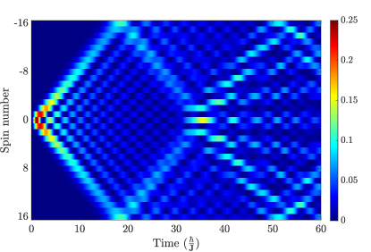
Figure 1: Exact evolution of entanglement after a local quench at $t=0$ in the middle of the chain obtained using the QCTF formulation. Due to periodic boundary condition and translational symmetry, all of the spins can be considered to be in the middle of the chain. The evolution shows clear light-cone behavior until quasi-particles arrive at the middle of the chain (located at the upper and lower edges of the figure).

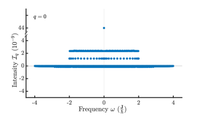
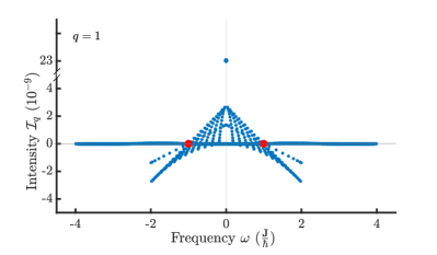
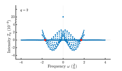
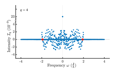
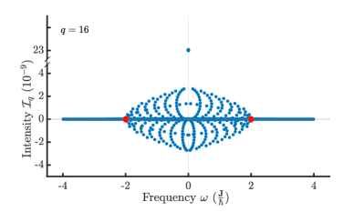
Figure 2: Entanglement frequency spectra for $q=0$ (initially excited spin) and further spins ($q$ denotes the distance). The spectra consist of two main classes of poles: dominant poles that contribute mainly to the entanglement evolution and suppressed poles, with intensities close to $\mathcal{I}_{q}=0$. For the initially excited spin ($q=0$), the dominant frequency spectrum consists of two equi-intensity lines of poles (refer to the main text for explanation). For further spins, the frequency spectra feature a string of poles close to the cut-off frequency ($\omega=\frac{2\mathbf{J}}{\hbar}$) that approach zero in intensity at $\approx 2\mathbf{J}\cos^{2}(\frac{pi}{4q})$ (these poles are marked by red circles), more rapidly for larger $q$. More generally, further spins exhibit spectra that are more oscillatory in intensity (see equation (10)), which leads to filtering out the fast modes in the entanglement dynamics and eventually to delayed development of entanglement.

Analysis- We will present two different analyses of equation (6), respectively in the frequency and time domains. The relation (6) shows that the entanglement frequency components (poles of $\tilde{\mathcal{Q}}_{q}(s)$) must be upper-bounded by $|s|<\frac{4\mathbf{J}}{\hbar}$. Importantly, as will be demonstrated, the frequencies in the upper half region, $\frac{2\mathbf{J}}{\hbar}<|s|<\frac{4\mathbf{J}}{\hbar}$, are highly (polynomially in $N$) suppressed and therefore negligible in the $N\rightarrow\infty$ limit. To produce these frequencies on the higher end of the spectrum, cooperative addition of all four terms in the frequency argument (i.e., $\cos(\frac{2\pi}{N}m_{i})$) is required, which necessarily rules that $m_{2}\neq m_{4}$. In this case, the inner summation over $p$ will lead to:

$$\sum_{p\neq q}e^{\frac{2i\pi}{N}\big{(}q(m_{1}-m_{3})+p(m_{4}-m_{2})\big{)}}=-e^{\frac{2i\pi}{N}q(m_{1}-m_{3}+m_{4}-m_{2})}.$$ (7)

Therefore, the inner summation reduces to a number with unit norm. Given the $N^{-4}$ scaling in $\tilde{\mathcal{Q}}_{q}(s)$, this situation not only suppresses all of the higher end frequencies ($\frac{\mathbf{2J}}{\hbar}<|s|<\frac{4\mathbf{J}}{\hbar}$), but also the majority of frequencies on the lower end ($0<|s|<\frac{2\mathbf{J}}{\hbar}$). As a result, the dominant frequencies correspond to $m_{2}=m_{4}$.

Entanglement of the initially excited spin (i.e., $q=0$) can be obtained directly from (6). In this case, the intensity of the dominant frequencies is proportional to their abundance. Thus, finding the intensity of each frequency component in the entanglement measure entails counting the instances when each particular frequency emerges as the four-tuple $(m_{1},m_{2},m_{3},m_{4})$ varies. This statement follows since the exponential term becomes unity when $q=0$ and $m_{2}-m_{4}=0$. As a result, the entanglement frequency spectrum of the initially excited spin ($q=0$) consists of two equal-intensity lines (see Figure 2), one for $m_{1}m_{3}\neq 0$, and one for $m_{1}m_{3}=0$, with lower intensity due to a lower number count.

Analogously, for the general case of $q\neq 0$, the dynamical measure (6) gives the propagation of entanglement throughout the chain. Here, the transient behavior of entanglement (corresponding to the fast time scales) is of main interest. Transient features of entanglement correspond to the poles close to $|s|\approx\frac{2\mathbf{J}}{\hbar}$, which can be verified to correspond to the following (note that all frequencies appear in positive and negative pairs; Here only positive frequencies are considered for brevity):

$$m_{2}=m_{4},(m_{1},m_{3})\approx(0,\pm\pi).$$ (8)

Therefore, the fastest dominant peak corresponds to:

$$(m_{1},m_{3})=(0,\pm\frac{N-1}{2}).$$ (9)

By employing the new set of variables $\epsilon=|m_{1}|-|m_{3}|-\frac{N}{2}$ and $\delta=|m_{1}|+|m_{3}|-\frac{N}{2}$, the intensity ($\mathcal{I}_{q}$) and frequency ($\omega_{q}$) of the (non-zero) dominant peaks are:

$$\mathcal{I}_{q}(\epsilon,\delta)\propto(-1)^{q}\Big{(}\cos(\frac{2\pi q}{N}\epsilon)+\cos(\frac{2\pi q}{N}\delta)\Big{)},$$ (10)

$$\omega_{q}(\epsilon,\delta)=\frac{2\mathbf{J}}{\hbar}\cos(\frac{\pi}{N}\epsilon)\cos(\frac{\pi}{N}\delta).$$ (11)

As a result, based on (10), one expects to observe a string of poles, close to and below the cut-off frequency ($\frac{2\mathbf{J}}{\hbar}$), the intensity of which decay to zero (and cross the horizontal axis in Figure 2) more rapidly as $q$ increases. A simple calculation shows that these crossings of the zero intensity line occur each time $|m_{1}|$ or $|m_{3}|$ crosses the pole near $\frac{N}{2}-\frac{N}{4q}$ and $\frac{N}{4q}$. Therefore, the first (meaning closest to the cut-off frequency) crossing corresponds to $m_{1}=\pm\frac{N-1}{2}$ and $|m_{3}|\approx\frac{N}{4q}$, which, according to (11), will be at the frequency (shown with red marks in Figure 2):

$$2\mathbf{J}\cos(\frac{\pi}{4q}-\frac{\pi}{2N})\cos(\frac{\pi}{4q}+\frac{\pi}{2N})\approx 2\mathbf{J}\cos^{2}(\frac{\pi}{4q}).$$ (12)

This mechanism filters out fast modes through the oscillatory behavior of poles near the cut-off frequency, leading to retarded growth of entanglement for farther spins (larger $q$). This behavior is analyzed in detail in the following paragraphs.

Here, we present an alternative and more in-depth analysis of the transient entanglement dynamics in the time domain. We demonstrate that entanglement of spins at the $q$’th distance from the initially quenched spin obeys the transient behavior $\sim(\frac{v_{e}t}{q})^{2q}$, where $v_{e}$ is a universal constant of the chain and describes the velocity of propagation for the entanglement edge. Given the even symmetry of the frequency components, the inverse Laplace transform of (6), which gives the entanglement dynamics of spin $q$, has the following general form in the time domain:

$$\mathcal{Q}_{q}(t)=\sum_{j}{\mathcal{I}_{q,j}\cos(\omega_{j}t)},$$ (13)

where $j$ is the index for all possible frequencies ($\omega_{j}=-is_{j}$, with $s_{j}$ being the poles of (6)), arising from the four-tuples $(m_{1},m_{2},m_{3},m_{4})$, and $\mathcal{I}_{q,j}$ is the intensity corresponding to $\omega_{j}$, when considering spin $q$. Therefore, all of the odd derivatives (with respect to time) of $\mathcal{Q}_{q}(t)$ at $t=0$ vanish and the even derivatives are:

$$\evaluated{\mathcal{Q}_{q}^{(2r)}(t)}_{t=0}=(-1)^{r}\sum_{j}{\mathcal{I}_{q,j}\omega_{j}^{2r}}.$$ (14)

We define the vector $\mathbf{\mathcal{I}}^{q}\doteq[\mathcal{I}_{q,1},\cdots,\mathcal{I}_{q,j},\cdots]^{T}$, thus, given that all of the first even (up to $2(q-1)$) derivatives of $\mathcal{Q}_{q}(t)$ vanish at $t=0$ we have the following linear system of equations:

$$V\mathcal{I}^{q}=\mathbf{0}$$ (15)

where $V$ is the following (transposed) Vandermonde matrix:

$$(V_{kj})\doteq(i\omega_{j})^{2(k-1)};k=1,\cdots,q.$$ (16)

Thus, the intensities in the entanglement dynamics of the $q$’th spin, i.e., $\mathcal{I}^{q}$, should belong to the null space of $V$. The proof of this statement can be found in the supporting material. Moreover, it is shown that the higher (than $2(q-1)$) order derivatives of $\mathcal{Q}_{q}(t)$, denoted by $\mathcal{Q}^{(2(q+\bar{k}))}_{q}(t)$, are:

$$\begin{split}\evaluated{Q_{q}^{(2(q+\bar{k}))}(t)}_{t=0}=&(\frac{\mathbf{J}}{2\hbar})^{2(q+\bar{k})}{(-1)^{\bar{k}}}\binom{2(q+\bar{k})}{\bar{k},q,q+\bar{k}}\\ &\times{\,{}_{2}F_{1}(-\bar{k},-\bar{k}-q;q+1;1)},\end{split}$$ (17)

where $\,{}_{2}F_{1}$ denotes the Gaussian hypergeometric function. Note that this expression is exact for $0\leq\bar{k}<q$ and, for larger $\bar{k}$’s, the contribution from suppressed poles in the entanglement frequency spectrum starts to emerge. The contributions of the suppressed poles are polynomially small in the entanglement’s transient behavior.

To study the transient behavior of entanglement, the lower order terms in the Taylor series expansion of (17) can be used. By transient, we are referring to the evolution of entanglement before the quasi-particles reach the $q$th distant spin, wherein entanglement is exponentially (in $q$) small, in accordance to the Lieb-Robinson theorem. For this purpose, The entanglement measure $Q_{q}(t)$ can be re-written in its asymptotic Taylor expansion form, which reveals an important feature of the entanglement dynamics: the faster than the group velocity propagation of entanglement in the system. Based on the fact that all lower (than $2q$th) derivatives of $Q_{q}(t)$ vanish, and using the Stirling’s approximation, $q!\approx\sqrt{2\pi q}(q/e)^{q}$, the leading term ($\bar{k}=0$) in the Taylor expansion of $Q_{q}(t)$ that governs the transient behavior of entanglement is:

$$\begin{split}\frac{1}{(q!)^{2}}(\frac{\mathbf{J}t}{2\hbar})^{2q}\approx\frac{1}{2\pi q}(\frac{t}{\tau_{q}})^{2q};\tau_{q}=\frac{2q\hbar}{\mathbf{J}e}.\end{split}$$ (18)

Accordingly, the following is the speed at which the edge of entanglement transports down the chain:

$$v_{e}=\frac{e\mathbf{J}}{2\hbar}=\frac{e}{2}v_{g}.$$ (19)

Therefore, $\tau_{q}=\frac{2q\hbar}{e\mathbf{J}}$ is the time before which entanglement is exponentially (in $q$) small for $q$th distant spin from the initially excited spin (see equation (18)). As we expect, $\tau_{q}$ depends linearly on $q$, when $q\gg 1$. Furthermore, by considering all orders of the Taylor series, the transient entanglement evolution, given by the hypergeometric function (17), can be approximated as follows (see the supplementary material for derivation):

$$Q_{q}^{transient}(t)\approx\alpha_{q}J_{2q}(\frac{2\mathbf{J}t}{\hbar}),$$ (20)

where $J_{2q}$ is a Bessel function of the first kind, of order $2q$ and $\alpha_{q}\doteq(4^{-q})\binom{2q}{q}$. We should note that since in (20), all terms in the Taylor series of $Q_{q}(t)$ are used, in comparison with (18), where only the leading term is used, this equation provides an enhanced approximation of the transient entanglement evolution up to time $\frac{\hbar}{\mathbf{J}}$, which is beyond the entanglement edge ($\tau_{q}$).

Summary - In this paper, we fully obtained the evolution of entanglement in an arbitrarily long Heisenberg spin chain after a local quench. The QCTF-based analysis allowed for the study of this phenomenon through a new lens. This method of analysis circumvented the calculation of the time evolution of the system’s state to obtain the entanglement measure $\tilde{\mathcal{Q}}_{q}(s)$ directly from the system’s Hamiltonian. Moreover, the QCTF allowed for detailed analysis in the frequency domain, in addition to an accompanying time-domain analysis, which revealed the velocity of the entanglement edge in this class of spin chains. This velocity, in addition to providing fundamental insight into the mechanism of correlation transport in Heisenberg chains, is of practical importance to quantum information processing technologies; Most significantly, this velocity prescribes the fastest rate at which information can be transported beyond quantum tunneling effects in quantum networks with similar effective dynamics.

A natural direction for future QCTF research, entails consideration of multi-magnon entanglement evolution in Heisenberg XXZ chains, which should provide insights into into the non-equilibrium quantum statistics in this class of system. Moreover, by implementing the “string hypothesis” of the Bethé ansatz in the QCTF framework, entanglement dynamics in Heisenberg chains can be studied in a variety of global quench settings, such as the tilted-ferromagnetic state [10]. Ultimately, we hope to use the QCTF framework to study the problem of entanglement propagation in Heisenberg chains with long-range interactions. This class of systems is not integrable and therefore requires further effort (e.g., employing time-independent perturbation theory) to handle.