Logical Bias Learning for Object Relation Prediction

Abstract

Scene graph generation (SGG) aims to automatically map an image into a semantic structural graph for better scene understanding. It has attracted significant attention for its ability to provide object and relation information, enabling graph reasoning for downstream tasks. However, it faces severe limitations in practice due to the biased data and training method. In this paper, we present a more rational and effective strategy based on causal inference for object relation prediction. To further evaluate the superiority of our strategy, we propose an object enhancement module to conduct ablation studies. Experimental results on the Visual Gnome 150 (VG-150) dataset demonstrate the effectiveness of our proposed method. These contributions can provide great potential for foundation models for decision-making.

1 Introduction

Scene graph generation (SGG) aims to generate a comprehensive textual graph that includes nodes representing object classes and edges denoting their pairwise relations. It has attracted significant attention due to its support for graph reasoning. Besides, it is also a good method to automatically generate pre-training data for foundation models. However, in recent years, there has been an evident decline in the number of cross-modal methods based on scene graphs. This suggests that the SGG task has deviated from practice, which is a confusing phenomenon as graph structures are widely and increasingly used in various tasks. After conducting a thorough investigation, we determine that the primary cause of this decline is the inefficiency of dealing with the relation bias problem.

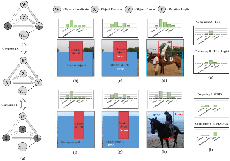
Figure 1: The illustration of the LBL strategy. (a) The causal graph for TDE w/o logic calculation. (b)&(f) Scenarios with masked object pairs’ bounding boxes. (c)&(g) Scenarios with masked object pairs’ bounding boxes and classes. (d)&(h) Scenarios with masked object pairs’ bounding boxes, classes and visual features. (e)&(i) are the TDE w/o logic scores for relation prediction of the two objects in (d)&(h), respectively.

The biased predictions arise from the long-tail distribution of data and the inclusion relationship among relations. In other words, this problem comes from a statistical perspective. Unfortunately, most existing methods manage to solve it via complex model designs, which are too specific and inefficient to be used in practice. Therefore, our proposal is to find a simple yet effective method. Subsequently, a superb strategy based on causal inference Glymour et al. (2016) is proposed, which is motivated by TDE Tang et al. (2020) and the phenomenon that students would ask their teacher for help if they are confused.

As shown in Fig. 1, given some choices, e.g., “on”, “riding”, “standing upside down”, you are required to describe the relation between two objects in the image. For Fig. 1 (b) and (f), most people would prefer to choose “on” between the two masked objects without visual and class information. It is inferred only from the object layout, namely the coordinate. Although relations like “on” and “near” are correct, they are useless for reasoning since the information is too rough. Naturally, we call this kind of bias “bad bias”.

If providing the object class information about the masked regions, i.e., given the classes for object1 and object2 as “person” and “horse” respectively as in Fig. 1 (c) and (g), we have the alternative word “riding” to represent their relation in this counterfactual scene. Because it matches our intuition that “riding” is common in the combination of “person” and “horse”. This inference comes from our common sense, which is rational Simon (1990) and in line with most cases. Hence, it is “good bias” relating to our logic thinking. We call it “logic bias”. It could provide extra knowledge and help with judgement when facing many uncertain choices.

Additionally providing the visual information, as shown in Fig. 1(h), the conclusion may be the same as the former. However, there also exists the case in Fig. 1 (d), where the scenario is unusual and the relation is described as “person standing upside down horse”. Total Direct Effect (TDE) Tang et al. (2020) is a strategy to solve this issue by empowering machines with the ability of counterfactual causality Pearl & Mackenzie (2018).

Fig. 1 (a) presents the underlying causal graphs of the above three alternate scenes. The arrow in $x$ → $y$ indicates that node $y$ is caused by node $x$. In relation prediction, there are three factors: object visual features ($X$), classes ($Z$) and coordinates ($W$); the faded links in the upper and bottom graphs denote the wiped-out factors are no longer caused by or affect their linked factors. These graphs offer an algorithmic formulation to calculate TDE.

The original TDE-based method Tang et al. (2020) predicts two scores. One is the relation prediction considering object visual, class, and coordinate information (e.g., Fig. 1 (d) and (h), represented by $X$+$Y$+$Z$). The other only considers object class and coordinate information (e.g., Fig. 1 (c) and (g), represented by $Y$+$Z$). The final score is their subtraction (Comparing A), aiming to predict the relations only through visual information ($X$) of subject and object without extra prior context. This operation can effectively reduce the “bad bias” and have a good effect for scenarios like Fig. 1 (d). However, it simultaneously reduce the “logical bias” for the common cases like Fig. 1 (h). Therefore, TDE may generate uncertainty since it reduces both bad bias and logic bias. The uncertainly predicted score are flatten as shown in Fig. 1 (i) Comparing A.

To address this issue, we propose a novel prediction strategy that utilizes knowledge when we encounter uncertainty estimation by TDE. We refer to this strategy as logical bias learning (LBL): when the results from pure visual information are uncertain for decision-making, try to use prior knowledge. It imitates the real scenario as aforementioned: students (TDE: $X$, Comparing A in Fig. 1(a)) would ask their teacher (TDE + Logic: $X$ + $Z$, Comparing B in Fig. 1(a)) for help if they are confused (uncertain). Hence, as shown in Fig. 1 (i), using TDE plus logic knowledge strategy when facing uncertainty predictions via the original TDE method, we could get results suppressing bad bias while highlighting the real one that matches our common sense. It perfectly corresponds to the logical reasoning process of humans.

Moreover, we are curious about the potential of this method, i.e., is it possible for normal students (bad performance on $X$) to surpass intelligent students (high performance on $X$) after learning this reasoning method (LBL)? To explore this, we furtuher present an agnostic object feature enhancement module (OEM). Current mainstream methods detect objects with bounding boxes, which may contain redundant and incorrect information from the background and other objects. An instance demonstrating this issue can be observed in Fig. 1 (d), where the horse’s bbox includes a partial person. This would seriously affect both detection and relation prediction. Inspired by the fact that text representation is much purer compared to images, OEM considers the object class as a query and enhances the targeted visual representations within bboxes through cross-attention. Meanwhile, deformable convolution Dai et al. (2017) is employed to effectively extract features from irregular objects. Afterwards, the feature patches are further processed through fine-grained attention, depending on their weights in the attention map.

In summary, our contributions are summarized as follows: 1) To solve the relation bias problem efficiently, a novel and effective prediction strategy, LBL, is proposed, which is deeply in line with human logical reasoning. Moreover, we present an object enhancement module to further verify the effectiveness of this strategy, demonstrating “normal students” can also outperform “intelligent students”. Note that LBL has potential for use in any model for decision-making. 2) Experiments on VG-150 indicate we make considerable improvements over the previous state-of-the-art methods.

2 Related Work

Scene Graph Generation. SGG aims to generate comprehensive summary graphs for images. It was first proposed by Johnson et al. (2015) in the cross-modal retrieval task. The increasing attention attracted by SGG shows its potential to support the image reasoning tasks Zhou et al. (2023); Yang et al. (2019); Liang et al. (2021); Zhou et al. (2022); Nguyen et al. (2021). There are two stages for the development process of the SGG. Early methods mainly focused on better visual networks Yin et al. (2018); Tang et al. (2019). After the bias problem was proposed by Zellers et al. (2018), many researchers turned to struggle for it Tang et al. (2020); Yang et al. (2022). However, the large cost of existing methods makes this problem not well solved and still far from practice.

Unbiased Training. There are two mainstream methods to solve the bias problem. 1) Labeling a new dataset or resampling existing ones. Like Geirhos et al. (2018), it posits that the primary cause of bias in SGG lies in the training data. This viewpoint is valid, but the high cost of annotation cannot be ignored. 2) Fusing the prior distribution of training sets. This category, such as Li et al. (2022); Lin et al. (2022), considers that incorporating the relation distribution from the training set into testing can help eliminate bias. But, the inadequacies of this approach become increasingly pronounced as the dataset undergoes changes. Besides them, there are few methods Tang et al. (2020); Dong et al. (2022) that take a different approach and are effective in addressing this problem. Our proposed approach falls within this category as well.

3 Method

In this section, we introduce the proposed method in detail. The overall pipeline is shown in Fig. 2. Given an image as input, we extract objects through the object detector. The detected object features are enhanced by the proposed OEM module, which consists of MLP, deformable convolution Dai et al. (2017) and multi-head self-attention (MHSA)Vaswani et al. (2017) blocks. Our model projects representations of entities (in our case, enhanced objects) as vectors in a learned common embedding space. Then, we adopt MOTIFS Zellers et al. (2018) as the encoder and a fully connected layer as the decoder to the list of projected features for relation probability prediction. The LBL strategy is applied to the estimated relation scores for final relation verification.

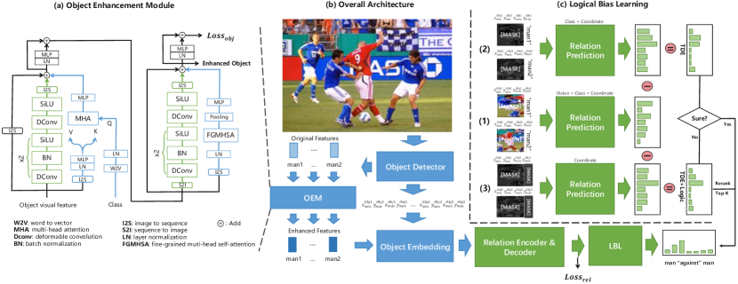
Figure 2: (a) The proposed object enhancement module. (b) The overall architecture of our model. (c) An illustration of the LBL strategy.

3.1 Object Enhancement Module

This module is intended to extract the important semantic information in the detected bounding box and achieve the similar effect of instance segmentation. We fuse the linguistic modal information of object class to refine the bounding box-level visual features through cross-attention operations.

For the first layer, we embed the object class word $x^{word}_{obj}$ (ground-truth when training and predicted one during test) by a 300-d FastText vector $x^{ft}_{obj}$. Then, we regard the text information $x^{ft}_{obj}$ as Q(uery), the visual feature $x^{vf}_{obj}$ as K(ey), and V(alue). To match their dimension, (64, 64)-d object visual feature is first divided into 8$\times$8 patches (each patch has 64-d). Then they are layer normalized and projected to 300-d. Finally, we project the (64, 300)-d matrix back to (64, 64)-d then to 4096-d for residual connection. The cross-attention can be summed up as:

$$Attention=\mathrm{Softmax}(\frac{x^{ft}_{obj}{x^{vf}_{obj}}^{\mathsf{T}}}{\sqrt{300}})x^{vf}_{obj}.$$ (1)

Some works Pan et al. (2022); Xu et al. (2021) have shown the effectiveness of the integration of attention and convolution for better feature representation. Therefore, we refer to the convolution part of ViTAE Xu et al. (2021) but replace the normal convolution with the deformable convolution Dai et al. (2017) for better concentration on the important parts of objects. The input and output dimensions of MLP remain the same (i.e., 4096 dimensions).

The second layer is a repetition of first layer except the attention mechanism. We use fine-grained multi-head self-attention (FGMHSA) to further extract the fine-grained features of object regions. Top-K important patches are selected based on the attention weights of patch tokens, and then they are split into smaller ones (one fourth) for better representation in a finer granularity. Further, these small patches are upsampled back to original size and tokenized as the input for attention operation. The output of FGMHSA contains more than 64 tokens. They are passed through a pooling layer and projected to 4096-d enhanced object feature $x_{eobj}^{vf}$. We use MLP to project the enhanced feature into $p$-d $x_{eobj}^{class}$ for the classification task. The cross-entropy loss is adopted:

$$Loss_{obj}=-\sum_{i=1}^{p}y_{i}\log({x_{eobj}^{class}}_{i}).$$ (2)

where $y$ is a $p$-d one-hot code denoting the ground truth of object class.

3.2 Object Embedding

Object Embedding. We project the enhanced object visual feature $x_{eobj}^{vf}$, embedded class feature $x^{ft}_{obj}$, and the 4-d bounding box coordinate $x^{bbox}_{obj}$: [$x_{min}/W$, $y_{min}/H$, $x_{max}/W$, $y_{max}/$ $H$] into the $d$-d space with three learned linear transforms (where $d$ is 2048). $W$ and $H$ are image width and height respectively. They are summed up as the final object embedding ${x_{obj}}$ as:

$$x_{obj}=LN(W_{1}x_{eobj}^{vf}+W_{2}x^{ft}_{obj})+LN(W_{3}x^{bbox}_{obj}),$$ (3)

where $W_{1}$, $W_{2}$ and $W_{3}$ are learned projection matrices. LN(·) is layer normalization Ba et al. (2016), added on the output of the linear transforms.

3.3 Relation Predication

For a given image, after detection and feature embedding, we could get a set of objects $\{\bm{x}_{obj}^{m}\}_{1:M}$.

Relation Encoder. The MOTIFS (BiLSTMs) Zellers et al. (2018) is used to encode the objects features. The encoded object is expressed as $x_{i}=BiLSTMs(x_{obj}^{i})$.

Relation Decoder. For each object pair, 4096-d union features $u_{ij}$ are extracted from their overlapped rectangle region to better utilize the context for relation prediction. We concatenate the encoded subject $x_{i}$ and object $x_{j}$ as [$x_{i}$; $x_{j}$], and then project this feature into 4096-d space to fit their union scale. Finally, we use a fully connected layer to predict their relation $R_{ij}$:

$$R_{ij}=\mathrm{argmax}(\mathrm{Softmax}(W_{8}(W_{7}([x_{i};x_{j}])\odot u_{ij})))$$ (4)

where $\odot$ indicates the element-wise product. The prediction loss is implemented in cross entropy as (2).

3.4 Logical Bias Learning (LBL)

The unbiased prediction lies in the difference between the observed factual outcome and its counterfactual alternate. The factual aspect contains object visual features and the context, i.e., their belonging classes and position relations. While the counterfactual aspect removes the real visual features. Fig. 2 (c) shows the comparison between them. In Fig. 2 (c), (1) represents the prediction result $Y_{x,z,w}$ using the vision $(x)$ $+$ class $(z)$ $+$ bbox $(w)$ features of objects; (2) shows the result $Y_{\bar{x},z,w}$ of using class $(z)$ $+$ bbox $(w)$ features; and (3) is the relation prediction distribution $Y_{\bar{x},\bar{z},w}$ of adopting the bbox $(w)$ features only. For the mask operation, we replace the original feature with a dummy value ($\bar{x}$ or $\bar{z}$), which is termed intervention in causal inference Glymour et al. (2016). Only the process of (1) is involved in the training period. Following the proposed LBL strategy, we obtain the TDE with logic (teacher): $Y_{T}$ = $Y_{x,z,w}-Y_{\bar{x},\bar{z},w}$ and the TDE without logic (student): $Y_{S}$ =$Y_{x,z,w}-Y_{\bar{x},z,w}$. When the prediction $Y_{S}$ encounters uncertainty, we get the result from $Y_{T}$ to re-rank. Otherwise, we directly use the result $Y_{S}$. The uncertainty is defined as: the predicted variance $V^{K}_{p}$ of top-K relations is smaller than the averaged $V^{K}$ in the training sets. In other words, if the confidence of the top-K results of $Y_{S}$ is similar, then go for $Y_{T}$ to re-rank the top-K relations. The final unbiased logits of $Y$ is formatted as:

$$\begin{cases}Y=Y_{S}&,\text{ if }V^{K}_{p}\geq V^{K}\\ Y=\mathrm{Rerank}(Y^{0:K}_{S}|Y_{T})+Y^{K:N}_{S}&,\text{ if }V^{K}_{p}<V^{K}\end{cases}$$ (5)

where $N$ is the total number of relations. Note that $K$ is set to 3 experimentally.

4 Experiments

4.1 Experimental Settings

Datasets. The experiments of SGG are conducted on two datasets, VG-150. We follow Zellers et al. (2018); Tang et al. (2020); Dong et al. (2022) to sample a 5k validation set from training set of VG-150 for parameter tuning.
Implementation details. Following Tang et al. (2020); Zhang et al. (2022), we employ a pre-trained Faster R-CNN Ren et al. (2015) with ResNeXt-101-FPN Xie et al. (2017) backbone for object detection. The BiLSTMs is used for relation encoding and a single fully connected layer for decoding. The top-K refers to the top-3 for the certain condition. The top-K important patches refer to the top 50% patches for the OEM. The 3$\times$3 kernel size is adopted for deformable convolution. Our model is implemented on the Pytorch platform with three RTX A5000 GPUs. We adopt the AdamW optimizer, set the batch size to 12, the initial learning rate to 1e-3 with the weight decay of 1e-4, and a linear decrease scheduler for a total of 40k steps.
Evaluation Metrics. We use mean Recall@K (mR@K), a widely used evaluation metric which computes the fraction of times the correct relation is predicted in the top K confident relation prediction, as the metrics for the following three tasks: 1) Predicate Classification (PredCls) provides objects with their corresponding bounding boxes, and requires models to predict the relation of the given pairwise objects; 2) Scene Graph Classification (SGCls) provides the ground-truth object bounding boxes, and needs the models to predict their classes and their pairwise relations. 3) Scene Graph Detection (SGDet) asks the models to detect all the objects and their bounding boxes, as well as predict the relationships of pairwise objects.

Table 1: Performance (%) of our method and other SOTA methods on VG-150.

Methods		PredCls			SGCls			SGDet
		mR@20	mR@50	mR@100	mR@20	mR@50	mR@100	mR@20	mR@50	mR@100
Specific	IMP Xu et al. (2017)	-	9.8	10.5	-	5.8	6.0	-	3.8	4.8
	KERN Chen et al. (2019)	-	17.7	19.2	-	9.4	10.0	-	6.4	7.3
	GBNet Zareian et al. (2020)	-	22.1	24.0	-	12.7	13.4	-	7.1	8.5
	PCPL Yan et al. (2020)	-	35.2	37.8	-	18.6	19.6	-	9.5	11.7
	BGNN Li et al. (2021)	-	30.4	32.9	-	14.3	16.5	-	10.7	12.6
Model-Agnostic	Motif Zellers et al. (2018)	11.7	14.8	16.1	6.7	8.3	8.8	5.0	6.8	7.9
	-TDE Tang et al. (2020)	18.5	25.5	29.1	9.8	13.1	14.9	5.8	8.2	9.8
	-IETrans Zhang et al. (2022)	-	35.8	39.1	-	21.5	22.8	-	15.5	18.0
	-GCL Dong et al. (2022)	30.5	36.1	38.2	18.0	20.8	21.8	12.9	16.8	19.3
	-OEM+LBL (ours)	27.4	32.3	35.5	16.9	19.7	21.0	13.1	17.1	19.7
	VCTree Tang et al. (2019)	13.1	16.7	18.1	9.6	11.8	12.5	5.4	7.4	8.7
	-TDE Tang et al. (2020)	18.4	25.4	28.7	8.9	12.2	14.0	6.9	9.3	11.1
	-IETrans Zhang et al. (2022)	-	37.0	39.7	-	19.9	21.8	-	12.0	14.9
	-GCL Dong et al. (2022)	31.4	37.1	39.1	19.5	22.5	23.5	11.9	15.2	17.5
	-OEM+LBL (ours)	29.6	34.9	38.5	17.6	20.8	24.0	13.2	16.7	18.1

4.2 Comparing with Other Methods

Since our proposed modules can be plugged into any other SGG approach, we compare our method with both specific and agnostic SOTA models. As shown in Tab. 1, we report the specific ones: IMP Xu et al. (2017), KERN Chen et al. (2019), GBNet Zareian et al. (2020), PCPL Yan et al. (2020) and BGNN Li et al. (2021); and agnostic ones based on MOTIFS Zellers et al. (2018) and VCTree Tang et al. (2019): TDE Tang et al. (2020), IETrans Zhang et al. (2022) and GCL Dong et al. (2022). On the widely used OCR-free dataset VG-150, we achieve compariable performance on PredCls and SGcls, and we establish a new state-of-the-art on SGDet, which is the most important metric for being applied to practice.

4.3 Ablation Study

To verify the effectiveness of our proposed modules, we conducted ablation experiments on models with and without OEM module and LBL strategy. Since LBL strategy contains two parts, i.e., TDE and TDE plus logic, to calculate the final prediction. We also compare the results with only using TDE or TDE+logic. (Note that TDE here is reproduced version)

Table 2: Ablations for various modules on VG-150

Module				PredCls (%)		SGCls (%)		SGDet (%)
OEM	TDE	Logic	LBL	mR@50	mR@100	mR@50	mR@100	mR@50	mR@100
✗	✓	✗	✗	23.6	27.7	12.4	14.1	8.0	9.6
✗	✓	✓	✗	20.6	26.4	11.8	15.6	10.9	12.4
✓	✓	✗	✗	24.0	27.7	12.6	16.4	11.6	14.6
✓	✓	✓	✗	26.3	30.4	15.3	18.2	12.6	15.0
✗	✓	✓	✓	28.6	32.5	16.6	19.6	12.8	15.4
✓	✓	✓	✓	32.3	35.5	19.7	21.0	17.1	19.7

As shown in Tab. 2, the performance of independent TDE with Logic and TDE (w/o Logic) is similar. However, after implementing our LBL strategy, significant improvements are made among the three tasks. Besides, LBL w/o OEM is better than TDE with OEM shows the powerful ability of the LBL strategy. It also verifies our aforementioned assumption that with teachers’ help (logic), normal students (TDE) may surpass intelligent students (TDE + OEM).

4.4 Qualitative Study

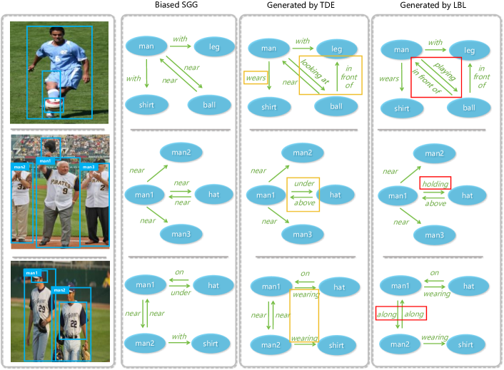
Figure 3: Examples of the visualized normal SGG and the unbiased ones generated by TDE&LBL.

We present three kinds of results qualitatively in Fig. 3. The blue circles represent objects. Relations are denoted by the green arrows. We can see that both TDE and LBL can well overcome the biased problem in (a): from “near” to “under” and “above” (labeled by yellow boxes). However, in scenarios (b) and (c), the aforementioned uncertain prediction by TDE takes place, but our strategy LBL can address it well (labeled by red boxes).

4.5 Specific Performance

Table 3: Specific results of mR@100 on VG-150

Relation Class	TDE as basic			Relation Class	TDE as basic
	+OEM+LBL	+OEM	TDE only		+OEM+LBL	+OEM	TDE only
above	0.1221	0.1471	0.0821	across	0.0000	0.0000	0.0000
against	0.1403	0.081	0.0000	along	0.1428	0.0612	0.0428
and	0.0318	0.0641	0.0059	at	0.1834	0.1881	0.1773
attached to	0.0275	0.0843	0.0556	behind	0.1713	0.1884	0.1742
belonging to	0.4309	0.3044	0.0602	between	0.0000	0.0000	0.0000
carrying	0.3638	0.2605	0.2565	covered in	0.0595	0.0202	0.0274
covering	0.0650	0.0860	0.0970	eating	0.4510	0.1378	0.1253
flying in	0.0000	0.0000	0.0000	for	0.0717	0.1079	0.0546
from	0.0000	0.0000	0.0000	growing on	0.0000	0.0000	0.0000
hanging from	0.0519	0.0687	0.0418	has	0.3008	0.2774	0.2874
holding	0.4510	0.2579	0.1916	in	0.1398	0.0994	0.0907
in front of	0.1751	0.2022	0.1713	laying on	0.2496	0.2548	0.1681
looking at	0.2330	0.2593	0.1502	lying on	0.1240	0.1378	0.0000
made of	0.0000	0.0000	0.0000	mounted on	0.0841	0.1469	0.0000
near	0.2352	0.3536	0.1598	of	0.2647	0.2781	0.2787
on	0.3079	0.1448	0.0640	on back of	0.0235	0.0355	0.0142
over	0.0428	0.0761	0.0372	painted on	0.1860	0.0000	0.0000
parked on	0.2616	0.1872	0.1557	part of	0.1595	0.1070	0.0000
playing	0.4165	0.0000	0.0000	riding	0.6510	0.4367	0.4537
says	0.1332	0.0000	0.0000	sitting on	0.3475	0.2091	0.1769
standing on	0.2572	0.1842	0.0690	to	0.0187	0.0246	0.0000
under	0.2218	0.2791	0.1419	using	0.3281	0.2437	0.1690
walking in	0.0466	0.0141	0.0000	walking on	0.1950	0.1084	0.0988
watching	0.4168	0.2326	0.2055	wearing	0.5735	0.4443	0.4763
wears	0.4312	0.3787	0.0000	with	0.1516	0.1289	0.0345

In Tab. 3, We show the mR@100 metric performance on each relation class. The results fully demonstrate the superiority of LBL (performance on most fine-grained relations is better), which is significantly beneficial for subsequent reasoning tasks. The total results are 19.68%, 14.60%, and 9.59% for (TDE+OEM+LBL), (TDE+OEM), and (TDE), respectively.

5 Discussion

In this paper, based on scene graph generation tasks, we delve into the potential of our proposed logical bias learning (LBL) strategy for object relation prediction. Meanwhile, an effective object feature enhancement module is proposed. Through extensive experiments, we demonstrate the superiority of our methods.
Moreover, we firmly believe that these contributions will significantly bridge the gap between the SGG and practical applications, which can further be beneficial for two aspects: 1) making it possible to automatically and efficiently generate high-quality cross-modal graph structural data, which can be used to pre-train foundation models; 2) directly being involved in the process of object relation prediction of any model. However, our methods have only been evaluated on SGG tasks. Therefore, more experiments on these aspects are needed in the future.

References

- Ba et al. (2016) Jimmy Lei Ba, Jamie Ryan Kiros, and Geoffrey E Hinton. Layer normalization. arXiv preprint arXiv:1607.06450, 2016.
- Chen et al. (2019) Tianshui Chen, Weihao Yu, Riquan Chen, and Liang Lin. Knowledge-embedded routing network for scene graph generation. In Proceedings of the CVPR, 2019.
- Dai et al. (2017) Jifeng Dai, Haozhi Qi, Yuwen Xiong, Yi Li, Guodong Zhang, Han Hu, and Yichen Wei. Deformable convolutional networks. In Proceedings of the ICCV, 2017.
- Dong et al. (2022) Xingning Dong, Tian Gan, Xuemeng Song, Jianlong Wu, Yuan Cheng, and Liqiang Nie. Stacked hybrid-attention and group collaborative learning for unbiased scene graph generation. In Proceedings of the CVPR, 2022.
- Geirhos et al. (2018) Robert Geirhos, Patricia Rubisch, Claudio Michaelis, Matthias Bethge, Felix A Wichmann, and Wieland Brendel. Imagenet-trained cnns are biased towards texture; increasing shape bias improves accuracy and robustness. arXiv preprint arXiv:1811.12231, 2018.
- Glymour et al. (2016) Madelyn Glymour, Judea Pearl, and Nicholas P Jewell. Causal inference in statistics: A primer. John Wiley & Sons, 2016.
- Johnson et al. (2015) Justin Johnson, Ranjay Krishna, Michael Stark, Li-Jia Li, David Shamma, Michael Bernstein, and Li Fei-Fei. Image retrieval using scene graphs. In Proceedings of the CVPR, 2015.
- Li et al. (2021) Rongjie Li, Songyang Zhang, Bo Wan, and Xuming He. Bipartite graph network with adaptive message passing for unbiased scene graph generation. In Proceedings of the CVPR, 2021.
- Li et al. (2022) Wei Li, Haiwei Zhang, Qijie Bai, Guoqing Zhao, Ning Jiang, and Xiaojie Yuan. Ppdl: Predicate probability distribution based loss for unbiased scene graph generation. In Proceedings of the CVPR, 2022.
- Liang et al. (2021) Weixin Liang, Yanhao Jiang, and Zixuan Liu. Graphvqa: Language-guided graph neural networks for scene graph question answering. NAACL-HLT 2021, 2021.
- Lin et al. (2022) Xin Lin, Changxing Ding, Jing Zhang, Yibing Zhan, and Dacheng Tao. Ru-net: regularized unrolling network for scene graph generation. In Proceedings of the CVPR, 2022.
- Nguyen et al. (2021) Kien Nguyen, Subarna Tripathi, Bang Du, Tanaya Guha, and Truong Q Nguyen. In defense of scene graphs for image captioning. In Proceedings of the ICCV, 2021.
- Pan et al. (2022) Xuran Pan, Chunjiang Ge, Rui Lu, Shiji Song, Guanfu Chen, Zeyi Huang, and Gao Huang. On the integration of self-attention and convolution. In Proceedings of the CVPR, 2022.
- Pearl & Mackenzie (2018) Judea Pearl and Dana Mackenzie. The book of why: the new science of cause and effect. Basic books, 2018.
- Ren et al. (2015) Shaoqing Ren, Kaiming He, Ross Girshick, and Jian Sun. Faster r-cnn: Towards real-time object detection with region proposal networks. Advances in neural information processing systems, 28, 2015.
- Simon (1990) Herbert A Simon. Bounded rationality. Utility and probability, pp. 15–18, 1990.
- Tang et al. (2019) Kaihua Tang, Hanwang Zhang, Baoyuan Wu, Wenhan Luo, and Wei Liu. Learning to compose dynamic tree structures for visual contexts. In Proceedings of the CVPR, 2019.
- Tang et al. (2020) Kaihua Tang, Yulei Niu, Jianqiang Huang, Jiaxin Shi, and Hanwang Zhang. Unbiased scene graph generation from biased training. In Proceedings of the CVPR, 2020.
- Vaswani et al. (2017) Ashish Vaswani, Noam Shazeer, Niki Parmar, Jakob Uszkoreit, Llion Jones, Aidan N Gomez, Łukasz Kaiser, and Illia Polosukhin. Attention is all you need. Advances in neural information processing systems, 2017.
- Xie et al. (2017) Saining Xie, Ross Girshick, Piotr Dollár, Zhuowen Tu, and Kaiming He. Aggregated residual transformations for deep neural networks. In Proceedings of the CVPR, 2017.
- Xu et al. (2017) Danfei Xu, Yuke Zhu, Christopher B Choy, and Li Fei-Fei. Scene graph generation by iterative message passing. In Proceedings of the CVPR, 2017.
- Xu et al. (2021) Yufei Xu, Qiming Zhang, Jing Zhang, and Dacheng Tao. Vitae: Vision transformer advanced by exploring intrinsic inductive bias. Advances in Neural Information Processing Systems, 34:28522–28535, 2021.
- Yan et al. (2020) Shaotian Yan, Chen Shen, Zhongming Jin, Jianqiang Huang, Rongxin Jiang, Yaowu Chen, and Xian-Sheng Hua. Pcpl: Predicate-correlation perception learning for unbiased scene graph generation. In Proceedings of the 28th ACM International Conference on Multimedia, 2020.
- Yang et al. (2022) Jingkang Yang, Yi Zhe Ang, Zujin Guo, Kaiyang Zhou, Wayne Zhang, and Ziwei Liu. Panoptic scene graph generation. In Proceedings of the ECCV. Springer, 2022.
- Yang et al. (2019) Xu Yang, Kaihua Tang, Hanwang Zhang, and Jianfei Cai. Auto-encoding scene graphs for image captioning. In Proceedings of the CVPR, 2019.
- Yin et al. (2018) Guojun Yin, Lu Sheng, Bin Liu, Nenghai Yu, Xiaogang Wang, Jing Shao, and Chen Change Loy. Zoom-net: Mining deep feature interactions for visual relationship recognition. In Proceedings of the ECCV, 2018.
- Zareian et al. (2020) Alireza Zareian, Svebor Karaman, and Shih-Fu Chang. Bridging knowledge graphs to generate scene graphs. In Proceedings of the ECCV. Springer, 2020.
- Zellers et al. (2018) Rowan Zellers, Mark Yatskar, Sam Thomson, and Yejin Choi. Neural motifs: Scene graph parsing with global context. In Proceedings of the CVPR, 2018.
- Zhang et al. (2022) Ao Zhang, Yuan Yao, Qianyu Chen, Wei Ji, Zhiyuan Liu, Maosong Sun, and Tat-Seng Chua. Fine-grained scene graph generation with data transfer. In Proceedings of the ECCV. Springer, 2022.
- Zhou et al. (2022) Xinyu Zhou, Shilin Li, Huen Chen, and Anna Zhu. Disentangled ocr: A more granular information for “text”-to-image retrieval. In Pattern Recognition and Computer Vision: 5th Chinese Conference, PRCV 2022, Shenzhen, China, November 4–7, 2022, Proceedings, Part I. Springer, 2022.
- Zhou et al. (2023) Xinyu Zhou, Anna Zhu, Huen Chen, and Wei Pan. Scene text involved” text”-to-image retrieval through logically hierarchical matching. In 2023 IEEE International Conference on Multimedia and Expo. IEEE, 2023.