Real-Time Risk Analysis with Optimization Proxies

Abstract

The increasing penetration of renewable generation and distributed energy resources requires new operating practices for power systems, wherein risk is explicitly quantified and managed. However, traditional risk-assessment frameworks are not fast enough for real-time operations, because they require numerous simulations, each of which requires solving multiple economic dispatch problems sequentially. The paper addresses this computational challenge by proposing proxy-based risk assessment, wherein optimization proxies are trained to learn the input-to-output mapping of an economic dispatch optimization solver. Once trained, the proxies make predictions in milliseconds, thereby enabling real-time risk assessment. The paper leverages self-supervised learning and end-to-end-feasible architecture to achieve high-quality sequential predictions. Numerical experiments on large systems demonstrate the scalability and accuracy of the proposed approach.

This research was partly supported by NSF award 2112533 and ARPA-E PERFORM award AR0001136.

I Introduction

The growing penetration of distributed energy resources (DERs) and of renewable generation, especially wind and solar generation, is causing a fundamental change of paradigm for power systems operations. Traditional approaches, where uncertainty is low and can be managed through reserve products, are no longer viable, in presence of significant wind and solar generation, and less predictable demand patterns due to DER adoption. Modern power grids thus require new operating practices that explicitly assess operational risk in real time.

Traditional approaches to risk assessment require running large numbers (typically in the thousands) of Monte-Carlo (MC) simulations. Risk and reliability metrics are then computed based on the outputs of these simulations [1]. In power systems, each MC simulation evaluates the behavior of the grid, e.g., generator setpoints and power flows, under a possible realization of load and renewable output, obtained from solving multiple economic dispatch problems sequentially (one per time step). Nevertheless, the computational cost of optimization, combined with the large number of MC simulations needed to obtain an accurate risk estimate, renders this workflow intractable for real-time risk assessment.

The paper proposes a new methodology, Risk Assessment with End-to-End Learning and Repair (RA-E2ELR), to address this computational challenge. RA-E2ELR replaces costly optimization solvers with fast E2ELR optimization proxies, i.e., differentiable programs that are guaranteed to produce near-optimal feasible solutions to economic dispatch problems [2]. RA-E2ELR is sketched in Figure 1 and is capable of assessing risk in electricity markets whose real-time operations are organized around economic dispatch processes that co-optimize energy and reserves. The paper reports numerical experiments on large-scale power grids with thousands of buses, demonstrating the scalability and fidelity of RA-E2ELR. To the best of the authors’ knowledge, RA-E2ELR is the first methodology to real-time risk assessment for the US market-clearing pipeline.

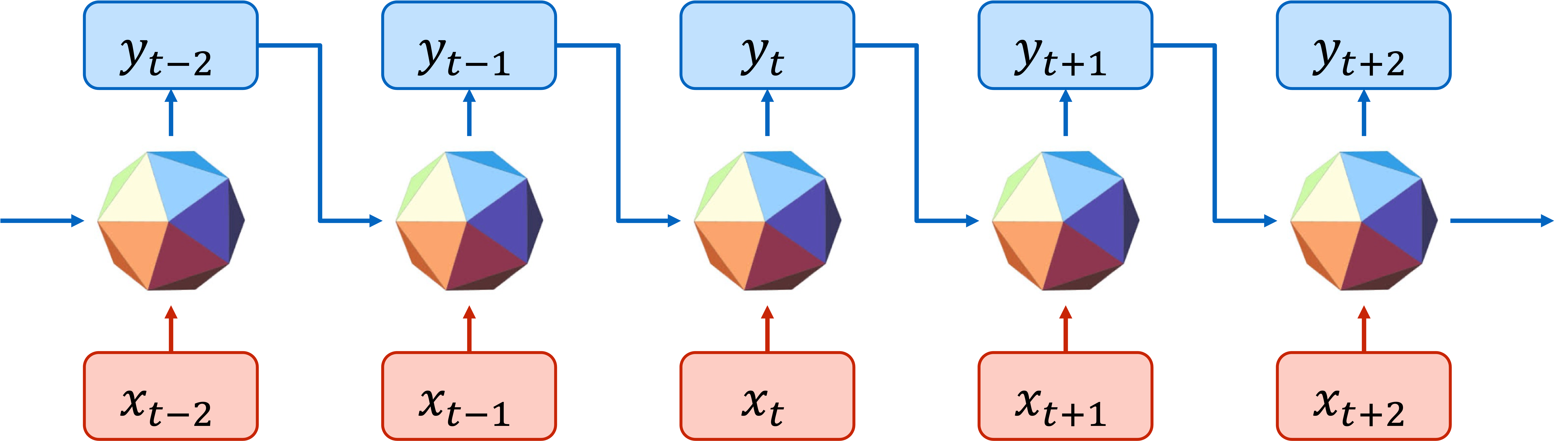
(a) Optimization-based Risk Assessment.

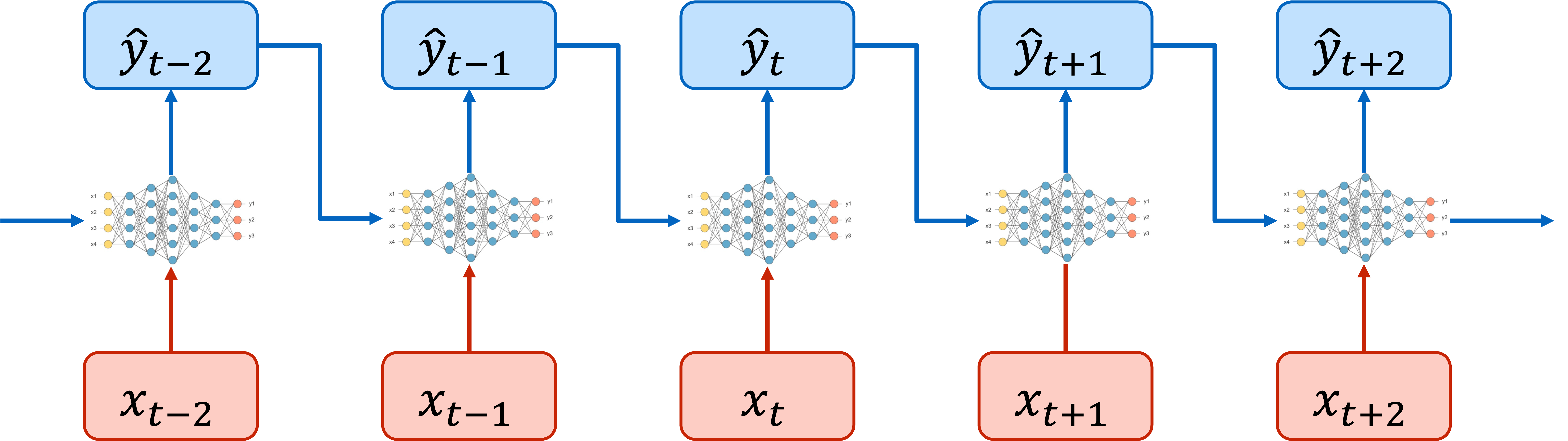
(b) Risk Assessment with E2ELR Proxies.

Figure 1: Illustration of the optimization-based (top) and RA-E2ELR MC simulation pipeline. At each step $t$, generator setpoints $y_{t}$ are decided based on current system conditions $x_{t}$ and previous setpoints $y_{t-1}$.

II Literature Review

II-A Risk Assessment in Power Systems

A number of reliability metrics have been proposed to quantify the risk in power systems explicitly such as Lack of ramp probability (LORP) [3], insufficient ramping resource expectation (IRRE) [4], loss of load expectation (LOLE) and expected unserved energy (EUE) [5]. More recently, Stover & al [1] proposed three levels of risk metrics for a quantity of interest: conditional value at risk, reliability, and risk. Computing those risk metrics is based on Monte Carlo (MC) sampling, which requires solving optimization instances for thousands of scenarios. These MC simulations are computationally expensive and intractable in real-time settings. This paper shows how to compute, in real-time, high-fidelity approximations of these risk metrics by leveraging E2ELR optimization proxies.

II-B Optimization Proxies for Sequential OPF

Some recent papers [6, 7, 8, 9, 10] focus on developing optimization proxies for multi-period ACOPF problems. They model the proxies with deep neural networks, typically combined with repair steps for feasibility. The proxies are trained under the framework of Reinforcement Learning (RL) with different algorithms. For instance, in [6], proxies are pretrained with imitation learning and then improved using proximal policy optimization. The results are reported for systems with up to 200 buses. In [7], the authors train proxies using deep deterministic policy gradient. The reward function is augmented with constraint violations to improve the feasibility. The results are reported on the 118-bus system. Those methodologies cannot guarantee feasibility and thus cannot be used for risk assessments.

Subsequent results addressed feasibility issues by designing complex optimization-based feasibility layers such as power flow solvers and convex-concave procedures [8], or holomorphic embedding [9]; they also use more advanced RL algorithms such as the soft actor-critic framework. Because of the complexity of their optimization-based repair steps, the improvements due to the proxies compared to the optimization algorithms are not sufficient for real-time risk assessment. The results are only reported up to systems with 300 buses.

III Operational Risk Assessment in Power Grids

Consider a power grid with buses $\mathcal{N}=\{1,...,N\}$, and branches $\mathcal{E}\,{=}\,\{1,...,E\}$. Assume, without loss of generality, that the costs are linear and that exactly one generator and one load are attached to each bus.

III-A The Economic Dispatch Formulation

Model 1 The Economic Dispatch Model.

Input: Current load $\mathbf{d}_{t}$, previous generation dispatch $\mathbf{p}_{t-1}$
Output: Generation dispatch $\mathbf{p}_{t}$

$$\min_{\mathbf{p}_{t}}\quad c^{\top}\mathbf{p}_{t}+M_{\text{th}}\|\xi_{\text{th}}\|_{1}$$ (1a)

s.t. $$\mathbf{e}^{\top}\mathbf{p}_{t}=\mathbf{e}^{\top}\mathbf{d}_{t}$$ (1b)

$$\mathbf{\underline{p}}\leq\mathbf{p}_{t}\leq\mathbf{\bar{p}}$$ (1c)

$$\mathbf{p}_{t-1}-R^{\downarrow}\leq\mathbf{p}_{t}\leq\mathbf{p}_{t-1}+R^{\uparrow}$$ (1d)

$$\mathbf{\underline{f}}-\xi_{\text{th}}\leq\Phi(\mathbf{p}_{t}-\mathbf{d}_{t})\leq\mathbf{\bar{f}}+\xi_{\text{th}}$$ (1e)

Model 1 presents the Economic Dispatch (ED) model to be solved at time step $t\,{\in}\,\mathbb{Z}$. For simplicity, the formulation omits the reserve constraints but RA-E2ELR has no difficulty in handling them [2]. The duration of each time step is assumed to be $1$; in the US, ED is solved every 5 minutes to clear the real-time electricity market. The ED problem at time $t$ takes, as inputs, the current demand $\mathbf{d}_{t}$ and the prior generation dispatch $\mathbf{p}_{t-1}$, and outputs the generation dispatch $\mathbf{p}_{t}$. For generators, the minimum output, maximum output, upward and downward ramping capacity are denoted by $\mathbf{\underline{p}}$, $\mathbf{\bar{p}}$, $R^{\uparrow}$ and $R^{\downarrow}$, respectively. The Power Transfer Distribution Factor (PTDF) matrix is denoted by $\Phi\,{\in}\,\mathbb{R}^{E\times N}$, and the lower and upper thermal limits are denoted by $\mathbf{\underline{f}}$ and $\mathbf{\bar{f}}$.

The ED objective (1a) minimizes the sum of total generation costs and thermal violation penalties. Constraint (1b) enforces power balance in the system. Constraints (1c) enforce generation minimum and maximum limits, and constraints (1d) enforce ramping constraints. Constraints (1c)–(1d) can be combined into

$$\mathbf{\underline{p}}_{t}\,{\leq}\,\mathbf{p}_{t}\,\leq\mathbf{\bar{p}}_{t},$$ (2)

where $\mathbf{\underline{p}}_{t}{=}\,\max\left(\mathbf{\underline{p}},\mathbf{p}_{t-1}{-}R^{\downarrow}\right)$ and $\mathbf{\bar{p}}_{t}{=}\,\min\left(\mathbf{\bar{p}},\mathbf{p}_{t-1}{+}R^{\uparrow}\right)$. Finally, constraints (1e) express thermal constraints using a PTDF formulation. Following the practice of US system operators [11], thermal constraints are treated as soft, i.e., thermal violations $\xi_{\text{th}}$ are penalized using a high price $M_{\text{th}}$.

III-B The Operational Risk Assessment Framework

Principled risk assessment is based on executing large numbers of MC simulations [1]. Each individual MC simulations emulates the system behavior under given (net) load conditions. The results of multiple MC simulations are then aggregated into risk and reliability metrics.

Formally, consider a simulation horizon $\mathcal{T}\,{=}\,\{1,...,T\}$. In a day-ahead setting, $\mathcal{T}$ may correspond to each hour of the operating day; in a real-time setting, $\mathcal{T}$ may capture the subsequent few hours at a 5-minute granularity. A set of scenarios $\mathcal{S}\,{=}\,\{1,...,S\}$, typically generated by a probabilistic forecasting model, is available. Algorithm 1 formalizes the simulation algorithm, which is also illustrated in Figure 1a. Each simulation $s$ takes as input a sequence of load $(\mathbf{d}^{s}_{1},...,\mathbf{d}^{s}_{T})$, where $\mathbf{d}^{s}_{t}$ denotes the vector of loads a time $t$ and for scenario $s$. At each time $t$, the minimum and maximum limits $\mathbf{\underline{p}}^{s}_{t},\mathbf{\bar{p}}^{s}_{t}$ are updated. Then, current generation dispatches $\mathbf{p}^{s}_{t}$ are computed by solving the ED problem in Model 1. Finally, the simulation returns the sequence of generation dispatches $(\mathbf{p}^{s}_{1},...,\mathbf{p}^{s}_{T})$.

Algorithm 1 Monte-Carlo Simulation

1:Demand scenario $(\mathbf{d}^{s}_{1},...,\mathbf{d}^{s}_{T})$

2:for $t=1\cdots T$ do

3:     $\mathbf{\bar{p}}^{s}_{t},\mathbf{\underline{p}}^{s}_{t}\leftarrow\max\left(\mathbf{\underline{p}},\mathbf{p}^{s}_{t-1}{-}R^{\downarrow}\right),\min\left(\mathbf{\bar{p}},\mathbf{p}^{s}_{t-1}{+}R^{\uparrow}\right)$

4:     $\mathbf{p}^{s}_{t}\leftarrow\text{ED}(\mathbf{d}^{s}_{t},\mathbf{\bar{p}}^{s}_{t},\mathbf{\underline{p}}^{s}_{t})$

5:end for

6:Return $(\mathbf{p}^{s}_{1},...,\mathbf{p}^{s}_{T})$

Risk metrics are computed by aggregating the outputs of multiple MC simulations, typically hundreds or thousands. This work considers the three levels of risk metrics proposed in [1]: conditional value at risk, probability of failure, and risk. Let $\mathcal{Q}$ be a so-called quantity of interest (QoI), whose value depends on the state of the system. Namely, denote by

$$Q^{s}_{t}=\mathcal{Q}(\mathbf{d}^{s}_{t},\mathbf{p}^{s}_{t})$$ (3)

the QoI value at time $t$ in scenario $s$. For instance, if $\mathcal{Q}$ is the system power imbalance, then $Q^{s}_{t}=\mathbf{e}^{\top}(\mathbf{p}^{s}_{t}-\mathbf{d}^{s}_{t})$.

III-B1 Conditional Value at Risk (CVAR)

Let $\alpha\,{\in}\,[0,1]$ be a given significance level, typically chosen by a system operator. The CVAR metric for time $t$ is

$$\text{CE}(\mathcal{Q}_{t})=\mathbb{E}[\mathcal{Q}_{t}|\mathcal{Q}_{t}\geq\mathcal{Q}_{t}(\alpha)]\approx\frac{\displaystyle\sum_{s\in\mathcal{S}}Q^{s}_{t}\cdot\mathbbm{1}_{Q^{s}_{t}\geq Q_{t}(\alpha)}}{\displaystyle\sum_{s\in\mathcal{S}}\mathbbm{1}_{Q^{s}_{t}\geq Q_{t}(\alpha)}},$$ (4)

where $\mathbbm{1}$ denotes the indicator function and $Q_{t}(\alpha)$ denote the $\alpha$ quantile of $(Q^{1}_{t},...,Q^{S}_{t})$. Note that the CVAR metric can be adapted to capture the left tail of the distribution [1].

III-B2 Probability of Failure

To assess system reliability, the second metric considers the probability of failure. Namely, let $\bar{Q}$ be a desired reliability threshold, i.e., the system is considered to fail if $\mathcal{Q}\geq\bar{Q}$. Then, the probability of failure at time $t$ is given by

$$\mathbb{P}(\mathcal{Q}_{t}\geq\bar{Q})\approx\frac{1}{S}\sum_{s\in\mathcal{S}}\mathbbm{1}_{Q^{s}_{t}\geq\bar{Q}}.$$ (5)

Note that reliability can be measured for the entire system, or for individual components.

III-B3 Risk

Risk quantifies the monetary consequences of failure. The risk at time $t$ is given by

$$\text{Risk}(\mathcal{Q}_{t})=\mathbb{E}[c(\mathcal{Q}_{t})]\approx\frac{1}{S}\sum_{s\in\mathcal{S}}c(Q^{s}_{t}),$$ (6)

where $c$ denotes a cost function. For instance, if the QoI $\mathcal{Q}$ denotes system power imbalance, a natural choice for $c$ could be $c\,{=}\,\text{VOLL}{\times}\mathcal{Q}$, where VOLL is the Value of Lost Load. Compared to the previous two metrics, risk captures the magnitude of adverse events and their financial consequences.

IV Risk Assessment With RA-E2ELR

The main limitation of existing risk assessment frameworks is their computational cost. Indeed, running thousands of simulations requires solving tens to hundreds of thousands of ED problems. This approach is not tractable, especially as more resources are integrated into the grid and the complexity of ED problems increases in the future.

IV-A Proxy-Based Risk Assessment

To enable fast risk assessment, the paper replaces costly optimization solvers with fast optimization proxies, i.e., differentiable programs that approximate the input-output mapping of optimization solvers. Figure 1b illustrates the proposed risk assessment framework, which replaces the ED optimization in step 3 of Algorithm 1 with an optimization proxy. At each time step $t$, the ED proxy takes as input the ED problem data $\mathbf{x}_{t}$, and outputs a near-optimal solution $\mathbf{\hat{y}}_{t}$ in milliseconds. It is important to note that, in the present setting, the proxy prediction at time $t$ is part of the input of the subsequent prediction. The sequential nature of the prediction task is in stark contrast with existing literature on optimization proxies, which consider individual ED instances.

The proxy-based risk assessment task can therefore be stated as follows. Given scenario $s$ with load $(\mathbf{d}^{s}_{1},...,\mathbf{d}^{s}_{T})$, the model should output a sequence $(\mathbf{\hat{p}}^{s}_{1},...,\mathbf{\hat{p}}^{s}_{T})$ of generator dispatches that is as close as possible to the sequence $(\mathbf{p}^{s}_{1},...,\mathbf{p}^{s}_{T})$ produced by an optimization solver.

Risk metrics can then be evaluated based on the predicted sequence $(\mathbf{\hat{p}}^{s}_{1},...,\mathbf{\hat{p}}^{s}_{T})$. Given a QoI $\mathcal{Q}$, let $\hat{Q}^{s}_{t}$ denote the value of the QoI in scenario $s$ at time $t$ given the predicted generation dispatches. Eqs. (4), (5), (6) then become

$$\text{CE}(\mathcal{Q}_{t}) \approx\frac{\displaystyle\sum_{s\in\mathcal{S}}\hat{Q}^{s}_{t}\cdot\mathbbm{1}_{\hat{Q}^{s}_{t}\geq\hat{Q}_{t}(\alpha)}}{\displaystyle\sum_{s\in\mathcal{S}}\mathbbm{1}_{\hat{Q}^{s}_{t}\geq\hat{Q}_{t}(\alpha)}},$$ (7)

$$\mathbb{P}(\mathcal{Q}_{t}\geq\bar{Q}) \approx\frac{1}{S}\sum_{s\in\mathcal{S}}\mathbbm{1}_{\hat{Q}^{s}_{t}\geq\bar{Q}},$$ (8)

$$\text{Risk}(\mathcal{Q}_{t}) =\mathbb{E}[c(\mathcal{Q}_{t})]\approx\frac{1}{S}\sum_{s\in\mathcal{S}}c(\hat{Q}^{s}_{t}),$$ (9)

where $\hat{Q}_{t}(\alpha)$ denotes the $\alpha$ quantile of $(\hat{Q}^{1}_{t},...,\hat{Q}^{S}_{t})$.

Observe that the proposed methodology predicts individual generation dispatches, resulting in a risk assessment for individual components compared to existing coarser-grained proposals, e.g., the zonal approach proposed in [12].

The proxies considered in this paper all extend the baseline DNN architecture shown in Figure 2. They differ in how they handle constraint violations. The baseline DNN consists of encoders, hidden layers, and a decoder. The DNN takes as input the load vector $\mathbf{d}$ and minimum/maximum limits $\mathbf{\underline{p}},\mathbf{\bar{p}}$, which are each fed to an encoder. The encoders are small multi-layer perceptron (MLP) models that use fully-connected layers with Rectified Linear Unit (ReLU) activation

$$\text{ReLU}(x)=\max(0,x).$$

The output of the encoders, referred to as embeddings, are passed to hidden layers, which are also fully connected layers with ReLU activations. A sigmoid activation is applied to the output of the last hidden layer, which yields a vector $\mathbf{z}\,{\in}\,[0,1]^{N}$. The sigmoid function is defined as

$$\sigma(x)=\frac{1}{1+e^{-x}}\in[0,1].$$ (10)

The predicted dispatch $\mathbf{\hat{p}}$ is then obtained as

$$\mathbf{\hat{p}}=\mathbf{z}\cdot\mathbf{\underline{p}}+(1-\mathbf{z})\cdot\mathbf{\bar{p}},$$ (11)

where all operations are element-wise. This approach ensures that $\mathbf{\underline{p}}\,{\leq}\,\mathbf{\hat{p}}\,{\leq}\,\mathbf{\bar{p}}$, which also ensures the feasibility of the ramping constraints due to the structure of Algorithm 7. However, the predicted dispatch may not satisfy power balance, i.e., $\mathbf{e}^{\top}\mathbf{\hat{p}}=\mathbf{e}^{\top}\mathbf{d}$ may not hold.

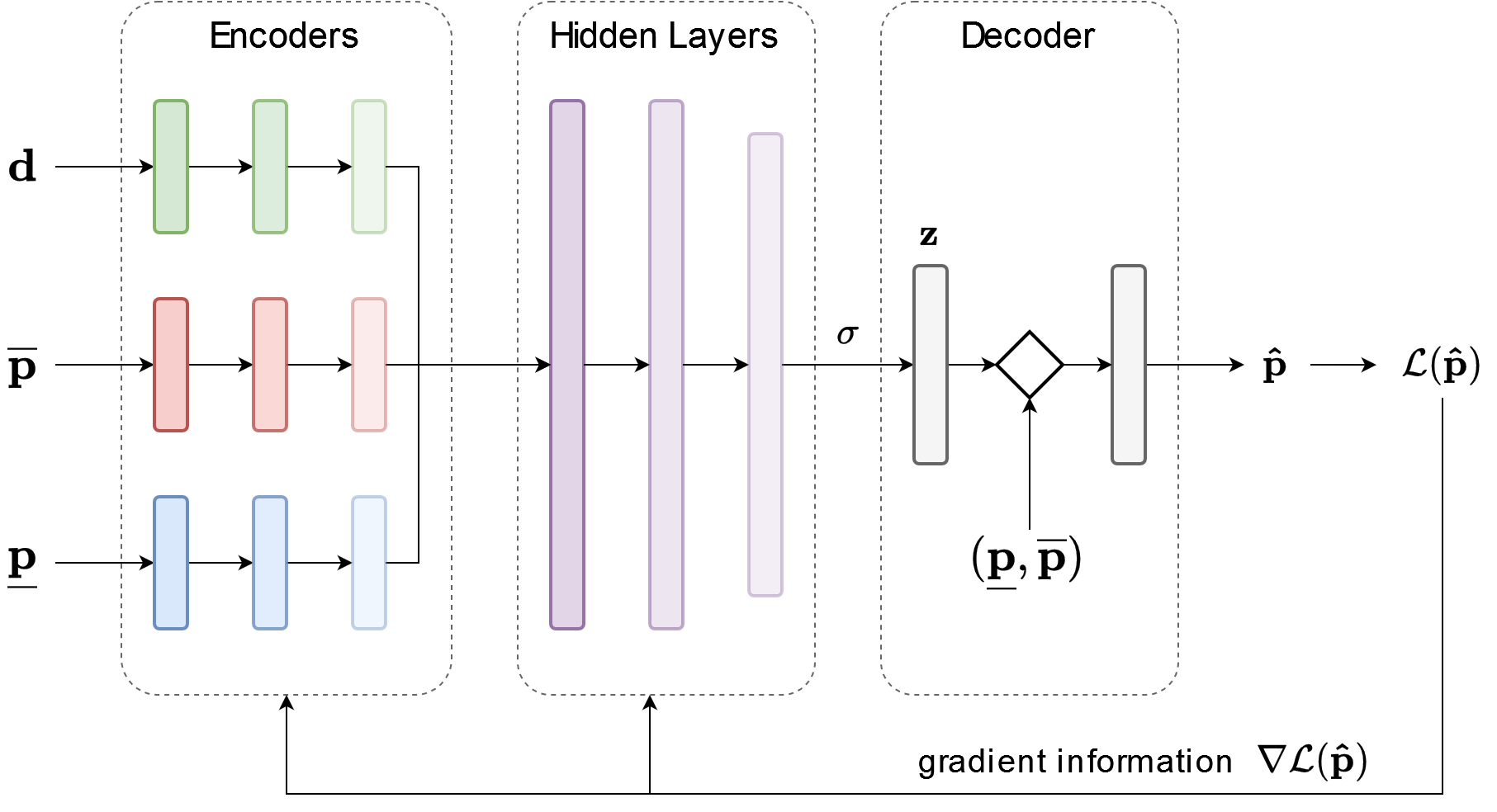
Figure 2: The Baseline DNN architecture. The hidden layers output $\mathbf{z}\,{\in}\,[0,1]^{N}$ using sigmoid activation $\sigma$, which is combined with min/max limits $\mathbf{\underline{p}},\mathbf{\bar{p}}$ to ensure $\mathbf{\underline{p}}\,{\leq}\,\mathbf{\hat{p}}\,{\leq}\,\mathbf{\bar{p}}$. The DeepOPF, DNN and E2ELR architectures extend the DNN architecture by adding a feasibility mechanism after the decoder.

IV-B The E2ELR Optimization Proxy

The E2ELR architecture [2] enforces min/max limits, power balance constraints, and reserve constraints via dedicated, differentiable feasibility layers. For the purpose of this paper, it is sufficient to present the repair layer for power balance, which is inserted between the approximation $\mathbf{\hat{p}}$ and the computation of the loss function. This repair layer takes $\mathbf{\hat{p}}$ as input and outputs

$$\begin{array}[]{rl}\mathbf{\tilde{p}}&=\left\{\begin{array}[]{ll}(1-\eta^{\uparrow})\mathbf{\hat{p}}+\eta^{\uparrow}\mathbf{\bar{p}}&\text{if }\mathbf{e}^{\top}\mathbf{\hat{p}}<\mathbf{e}^{\top}\mathbf{d}\\ (1-\eta^{\downarrow})\mathbf{\hat{p}}+\eta^{\downarrow}\mathbf{\underline{p}}&\text{if }\mathbf{e}^{\top}\mathbf{\hat{p}}\geq\mathbf{e}^{\top}\mathbf{d}\end{array}\right.\end{array}$$ (15)

where $\mathbf{\underline{p}}\,{\leq}\,\mathbf{\hat{p}}\,{\leq}\,\mathbf{\bar{p}}$, and $\eta^{\uparrow}$, $\eta^{\downarrow}$ are defined as follows:

$$\eta^{\uparrow} =\frac{\mathbf{e}^{\top}\mathbf{d}-\mathbf{e}^{\top}\mathbf{\hat{p}}}{\mathbf{e}^{\top}\mathbf{\bar{p}}-\mathbf{e}^{\top}\mathbf{\hat{p}}}, \eta^{\downarrow} =\frac{\mathbf{e}^{\top}\mathbf{\hat{p}}-\mathbf{e}^{\top}\mathbf{d}}{\mathbf{e}^{\top}\mathbf{\hat{p}}-\mathbf{e}^{\top}\mathbf{\underline{p}}}.$$ (16)

The repaired dispatch $\mathbf{\tilde{p}}$ is feasible if and only if ED is feasible (see Theorem 1 in [2]).

IV-C The Training Methodology

The training of E2ELR is based on self-supervised learning [13, 2], which directly minimizes the objective function (1a). Consider a dataset with $M$ data points

$$\mathcal{D}=\Bigl{\{}\mathbf{x}^{1},\mathbf{x}^{2},\cdots,\mathbf{x}^{M}\Bigl{\}},$$ (17)

where $\mathbf{x}^{t}=\{\mathbf{d}^{t},\mathbf{\bar{p}}^{t},\mathbf{\underline{p}}^{t}\}$, Let $f_{\boldsymbol{\Theta}}$ be the machine learning model with trainable parameters $\boldsymbol{\Theta}$. The training of $f_{\boldsymbol{\Theta}}$ amounts to solving the optimization problem

$$\boldsymbol{\Theta}^{*}=\operatorname*{arg-min}_{\boldsymbol{\Theta}}\frac{1}{M}\sum^{M}_{t=1}\mathcal{L}(f_{\boldsymbol{\Theta}}(\mathbf{x}^{t})),$$ (18)

In E2ELR, the loss function is the objective function of ED:

$$\mathcal{L}(\mathbf{\hat{p}}) =c(\mathbf{\hat{p}})+M_{\text{th}}\|\xi_{\text{th}}(\mathbf{\hat{p}})\|_{1}.$$ (19)

Observe that E2ELR only uses a set of inputs for training: it does not require labeled data.

V Experimental Results

V-A The Machine Learning Architectures

A key advantage of RA-E2ELR is its ability to produce ED-feasible solutions quickly at each stage of the MC simulations. To demonstrate these benefits, the paper compares RA-E2ELR to other ML architectures, which offer no feasibility guarantees. To train these infrastructures, the loss function should be generalized to $\mathcal{L}(\mathbf{\hat{p}})=\varphi(\mathbf{\hat{p}})+\lambda\psi(\mathbf{\hat{p}})$, where the first term $\varphi(\mathbf{\hat{p}})$ is the objective value of ED

$$\varphi(\mathbf{\hat{p}}) =c(\mathbf{\hat{p}})+M_{\text{th}}\|\xi_{\text{th}}(\mathbf{\hat{p}})\|_{1}$$ (20)

and the second term $\psi(\mathbf{\hat{p}})$ penalizes constraint violations. For instance, the power balance violations can be formalized as

$$\psi(\mathbf{\hat{p}})=M_{\text{pb}}|\mathbf{e}^{\top}\mathbf{d}-\mathbf{e}^{\top}\mathbf{\hat{p}}|,$$ (21)

where $M_{\text{pb}}$ are penalty coefficients.

The evaluation considers three ML architectures to show the benefits of RA-E2ELR: the baseline DNN architecture presented earlier, Deep-OPF [14], and DC3 [15].

V-A1 DeepOPF

The DeepOPF architecture [14] extends the DNN model by adding a equality completion step that enforces system power balance (1b). Let $\mathbf{\hat{p}}$ denote the output of DNN and assume bus $1$ is the slack bus without loss of generality. The equality completion layer outputs $\mathbf{\tilde{p}}\,{\in}\,\mathbb{R}^{N}$, where

$$\mathbf{\tilde{p}}_{1} =\mathbf{e}^{\top}\mathbf{d}-\sum_{i>1}\mathbf{\hat{p}}_{i},\ \mathbf{\tilde{p}}_{i} =\mathbf{\hat{p}}_{i},\ \forall i>1,$$ (22)

thus ensuring the satisfaction of the power balance constraint (1b). However, the dispatch of the slack generator $\mathbf{\tilde{p}}_{1}$ is not guaranteed to respect its minimum and maximum limits.

V-A2 Deep Constraint Completion and Correction (DC3)

The DC3 architecture [15] uses the same equality completion mechanism as DeepOPF, with an additional inequality correction step. The latter mitigates potential violations of the min/max limits for the slack generator, and uses unrolled gradient descent mechanism that minimizes the violation of inequality constraints. The number of gradient steps in the correction mechanism is set to a fixed value $K$. If $K$ is large enough, then DC3 returns feasible solutions, albeit at the cost of longer inference times. A smaller $K$ improves inference time, but may yield constraint violations.

V-B Data Generation

Experiments are carried on the IEEE 300-bus system (ieee300) [16] and the Pegase 1354-bus system (pegase1k) [17], using data from the UnitCommitment (UC) package [18]. The experiments use the network topology and cost information in the original test cases. Load time series and the minimum/maximum limits and ramping rates of the generators are obtained from [18]. For ease of presentation, all generators are assumed to be online; the proposed framework naturally extends to varying commitment decisions. For each system, [18] provides 365 benchmark instances, one per day in 2017, with each instance spanning a horizon of $T\,{=}\,36$ hours. This initial dataset of 365 load profiles is augmented by generating addition load samples, using the methodology proposed in [19].

For a given system and a given day, bus-level load scenarios are of the form $\mathbf{d}_{i,t}=\xi_{i,t}\times(\gamma_{t}\times\bar{P}^{d}),$ where $\bar{P}^{d}$ denotes the maximum total load in the reference UC instance, $\gamma\,{\in}\,\mathbb{R}^{T}$ captures the distribution of load-to-peak ratio, and $\xi_{i,t}$ denotes bus-level scaling factors. The distribution of $\gamma$ is estimated from the original 365 instances using a Gaussian copula model with Beta marginal distributions. Note that, in the instances provided by [18], each bus $i$ always accounts for a fixed proportion $\xi^{\text{ref}}_{i}$ of total demand. Therefore, nodal disaggregation factors $\xi$ are of the form $\xi_{i,t}\,{=}\,\xi^{\text{ref}}_{i}\,{\times}\,\eta_{i,t}$, where $\eta_{i,t}$ is uncorrelated white noise with log-normal distribution of mean $1$ and 5% standard deviation.

Figure 3 depicts daily total load scenarios for the ieee300 and pegase1k systems. The paper selected August 22nd, 2017 for ieee300, which was found to encounter capacity shortages, and July 13th, 2017 for pegase1k, which is the day that experienced the highest load over the year. A total of 1024 and 2048 scenarios are generated for the 300 and 1354-bus system, respectively. Each dataset is then split between training (80%), validation (10%) and testing (10%).

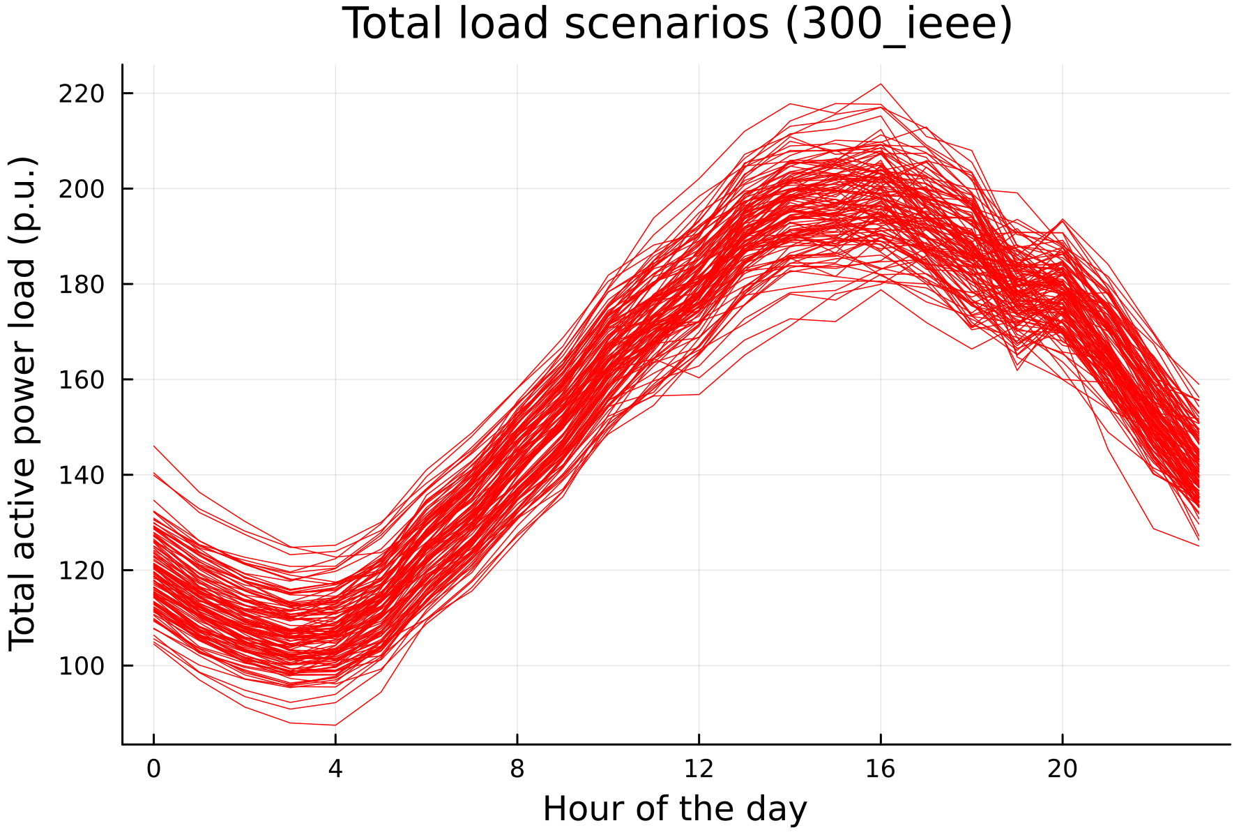
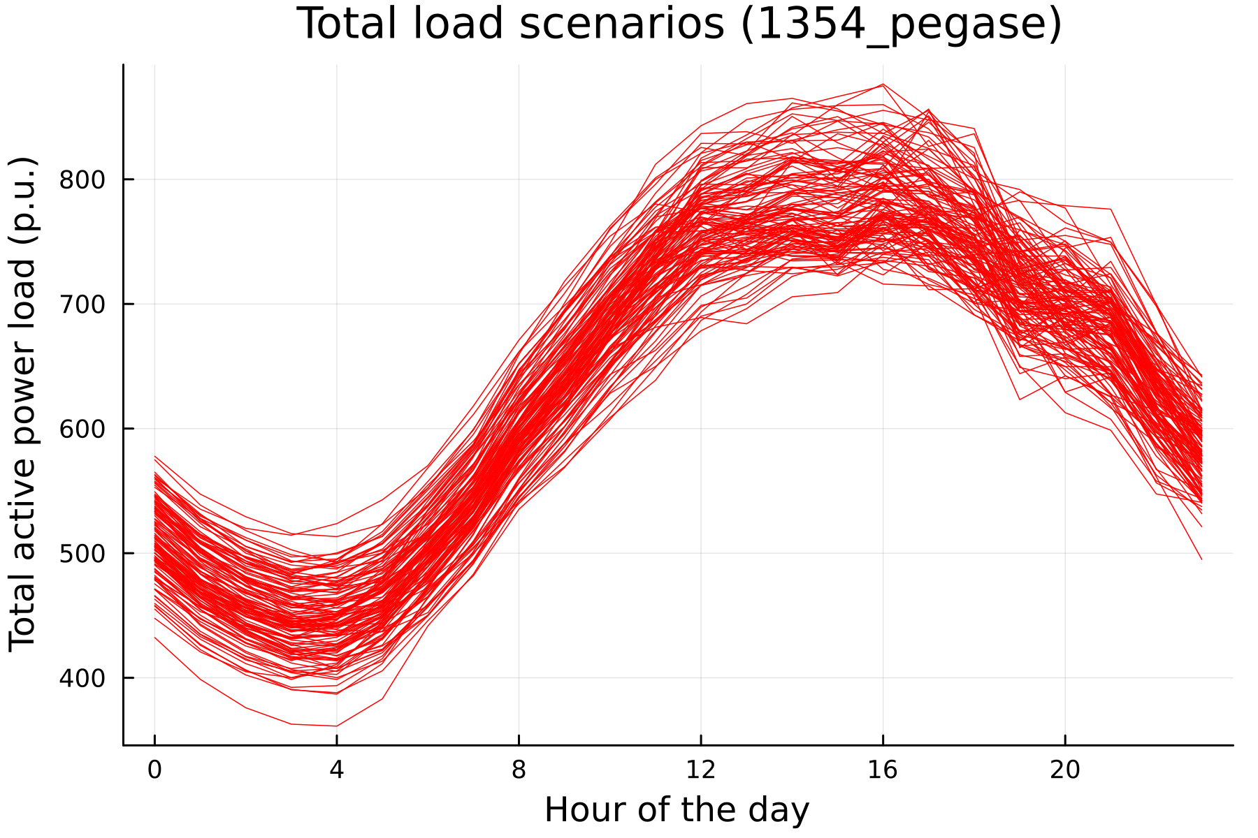
Figure 3: Total load scenarios used in the experiments. Left: ieee300, on August 22nd, 2017. Right: pegase1k, on July 13th, 2017.

V-C Implementation Details

The optimization problems are formulated in Julia using JuMP [20], and solved with Gurobi 9.5 [21], with a single CPU thread and its default parameters. All deep learning models are implemented using PyTorch [22] and trained using the Adam optimizer [23]. All models are hyperparameter tuned using a grid search, with the learning rate from $\{10^{-2},10^{-3}\}$, hidden dimension from $\{128,256\}$ and penalty term of constraint violation from $\{0.1,1\}$. For each system, the model with the lowest validation loss is selected and the performances on the test set are reported. During training, the learning rate is reduced by a factor 10 if the validation loss shows no improvement for a consecutive sequence of 10 epochs. In addition, training is stopped if the validation loss does not improve for consecutive 20 epochs. Experiments are conducted on dual Intel Xeon 6226@2.7GHz machines running Linux, on the PACE Phoenix cluster [24]. The ML models are trained on Tesla V100-PCIE GPUs with 16GBs HBM2 RAM.

V-D Comparison Framework

The risk simulations follow Algorithm 1. Since all simulations start from the same initial generation setpoint, ramping issues may arise at the beginning of the simulation, which results in artificially high risk during the first few hours of the day. Therefore, results are reported for a 24-hour period starting at 4am and ending at 4am. Finally, to ensure fair comparison between all ML models, the paper implements the following mechanism. All generation dispatches are clipped, if necessary, to ensure that minimum/maximum limits (2) are satisfied. This mechanism is executed at each time step of every simulation, and captures the fact that generators cannot adjust their output beyond their physical capabilities. While this does not affect the output of DNN and E2ELR, it may modify the output of DeepOPF and DC3, thus resulting in power balance violations instead of violations of the slack bus constraints.

V-E Global Risk Analysis

Figures 4 and 5 compare ground truth and proxy-based risk profiles for the ieee300 and pegase1k systems, respectively. The ground truth risk profiles are obtained by executing Algorithm 1 with an optimization solver (GRB). The proxy-based risk profiles are obtained by replacing the optimization solver with an optimization proxy. Each figure reports, for each hour: the 90%-CVaR (level 1) for system-wide power imbalance and total thermal violations, the probability of system-wide power imbalance and thermal violations, and the risk of power imbalance and total thermal violations.

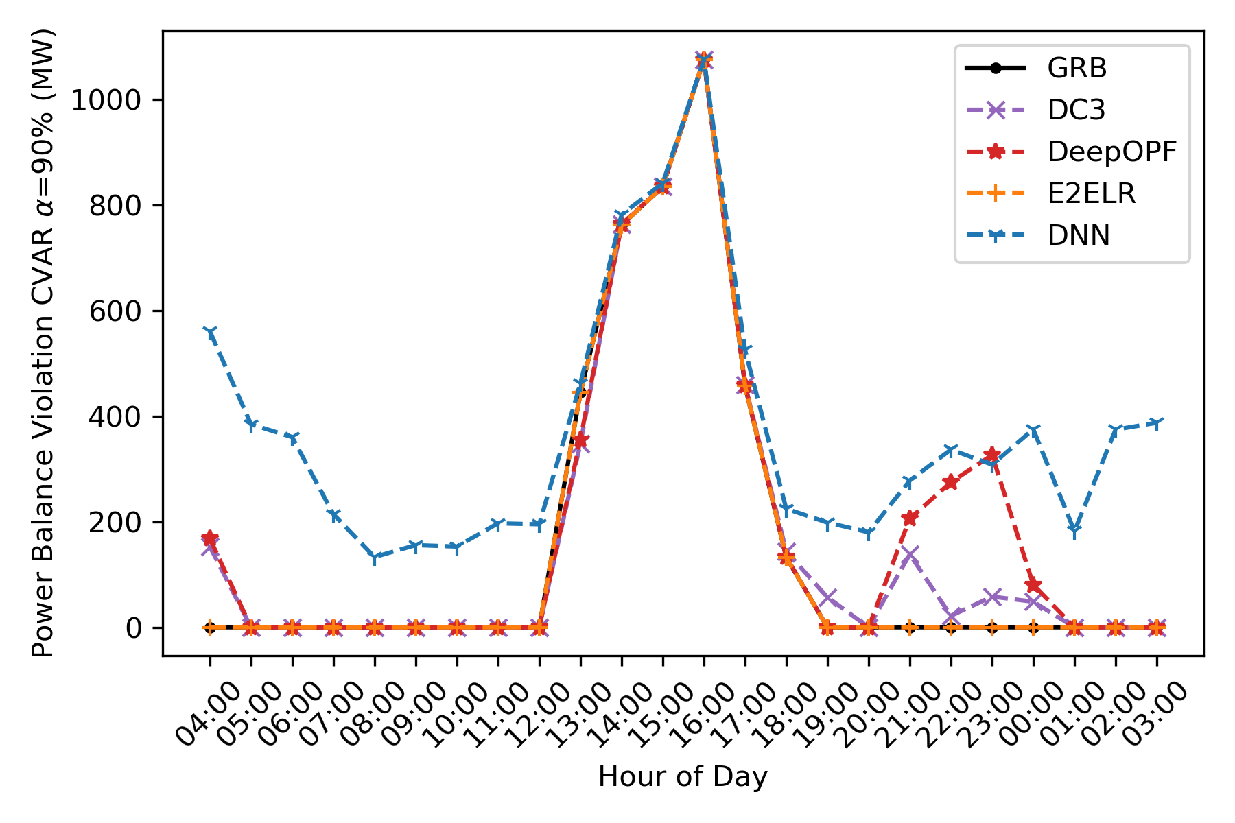
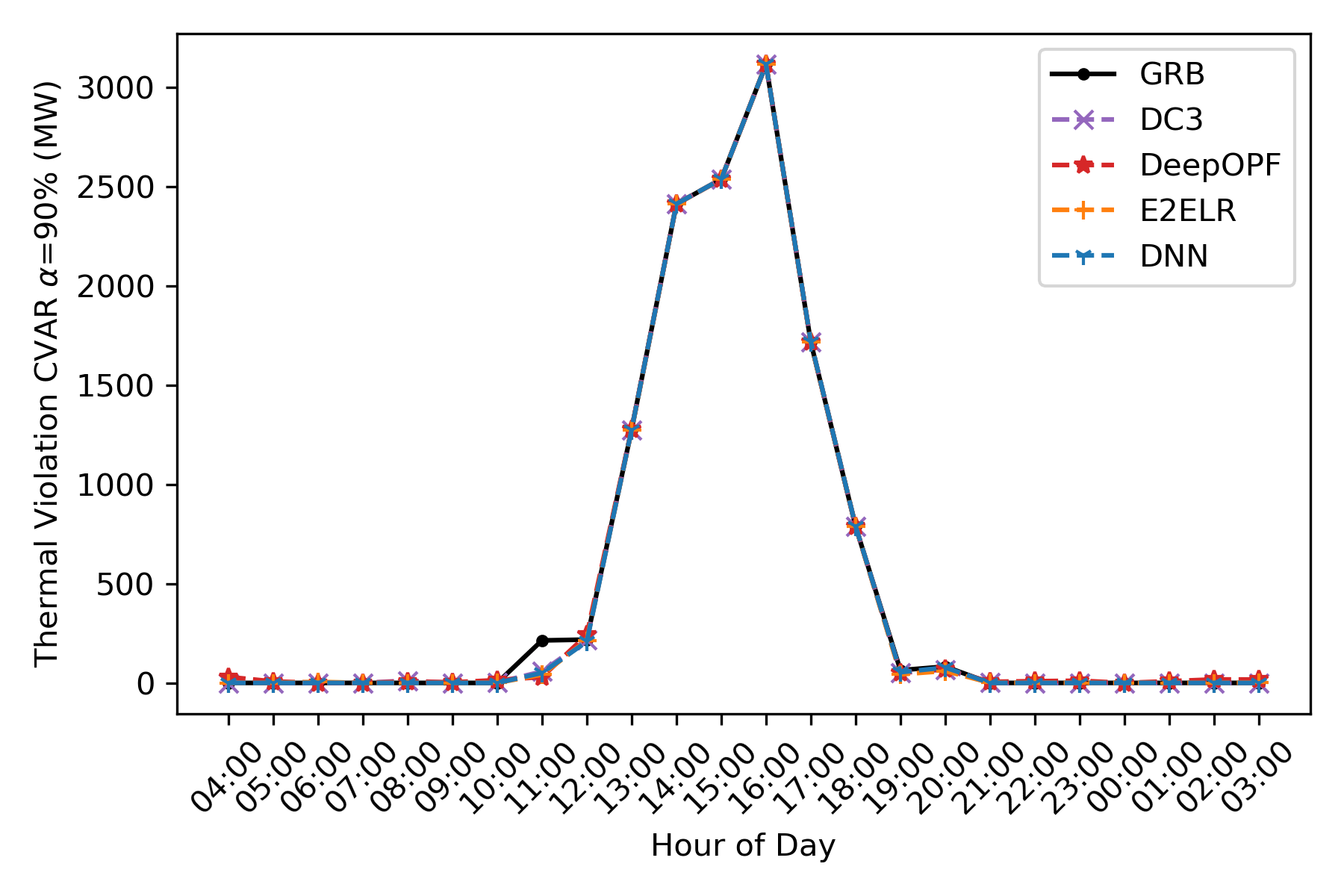
(a) Level-1 (CVaR) risk metrics for ieee300. Left: $\text{CVaR}_{90\%}$ of system power imbalance. Right: $\text{CVaR}_{90\%}$ of total thermal violations.

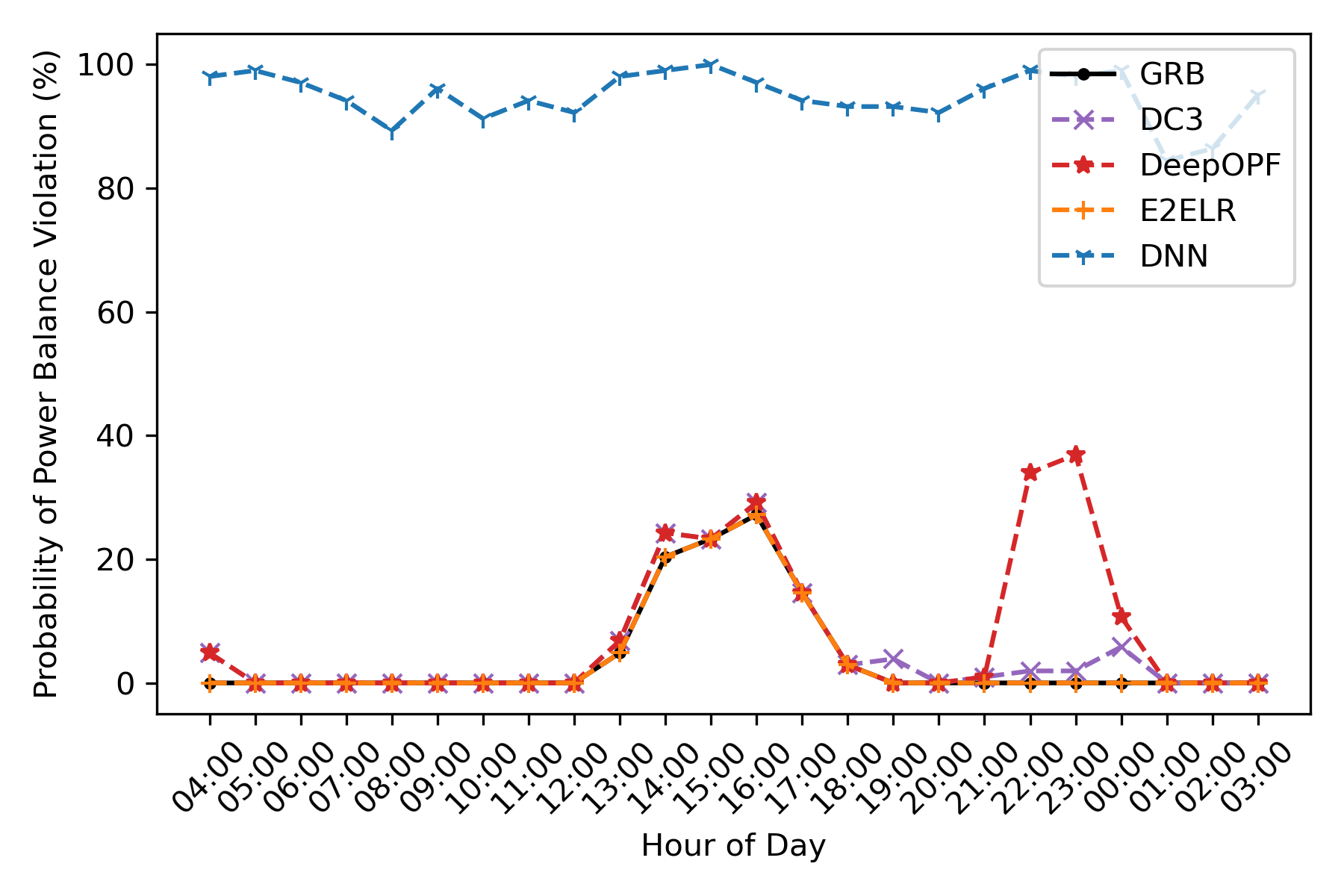
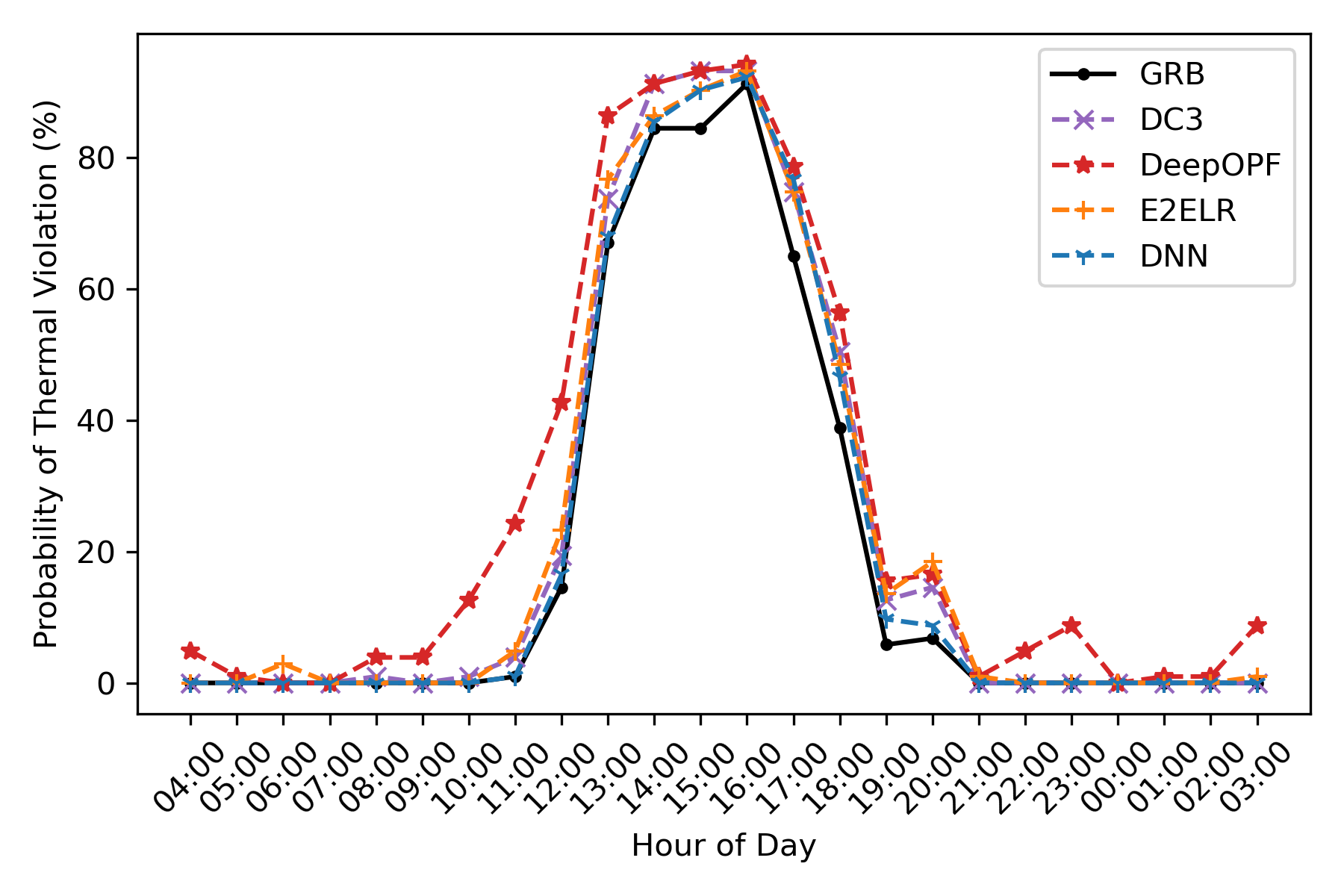
(b) Level-2 (probability of adverse event) risk metrics for ieee300. Left: probability of system power imbalance. Right: probability of non-zero total thermal violations.

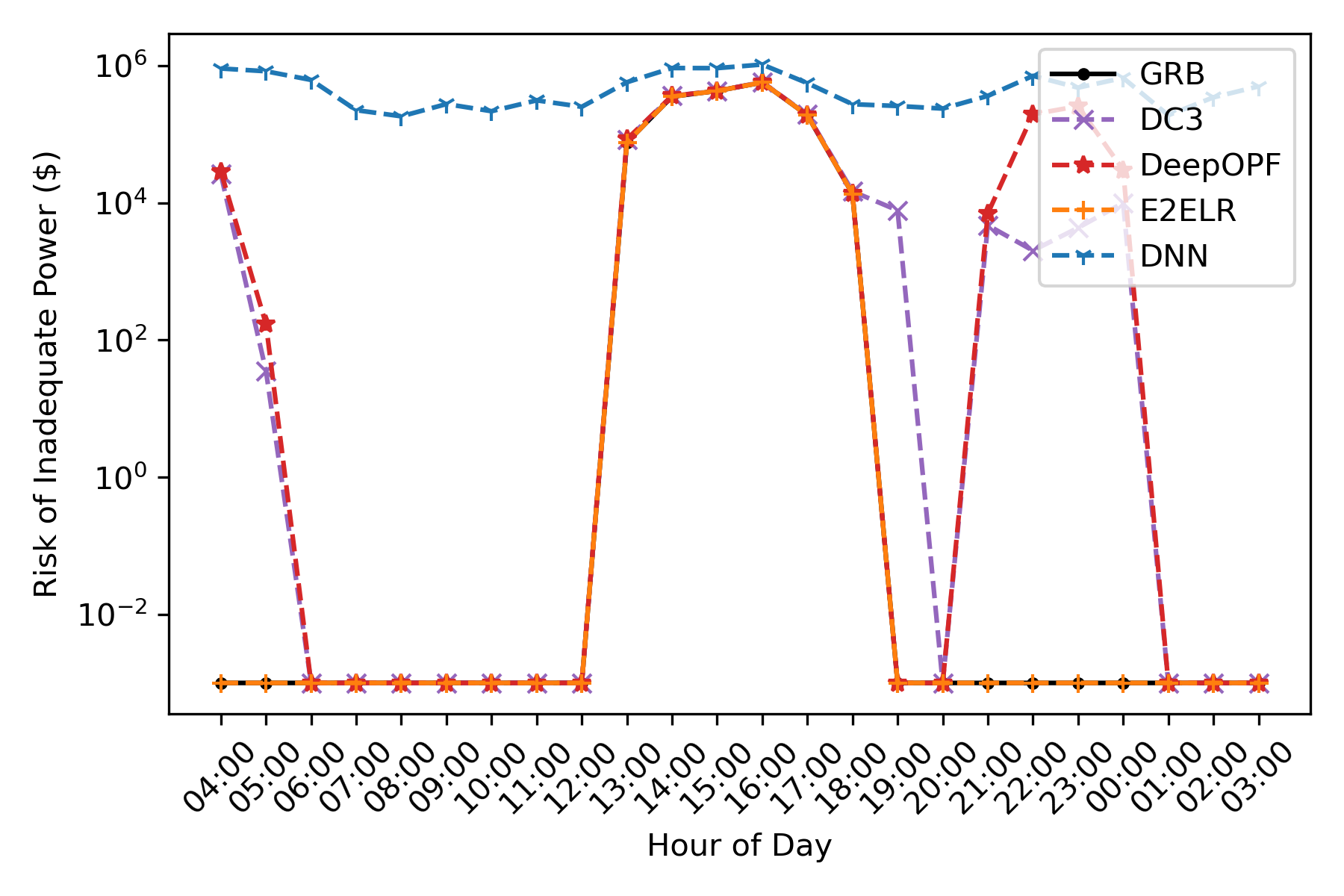
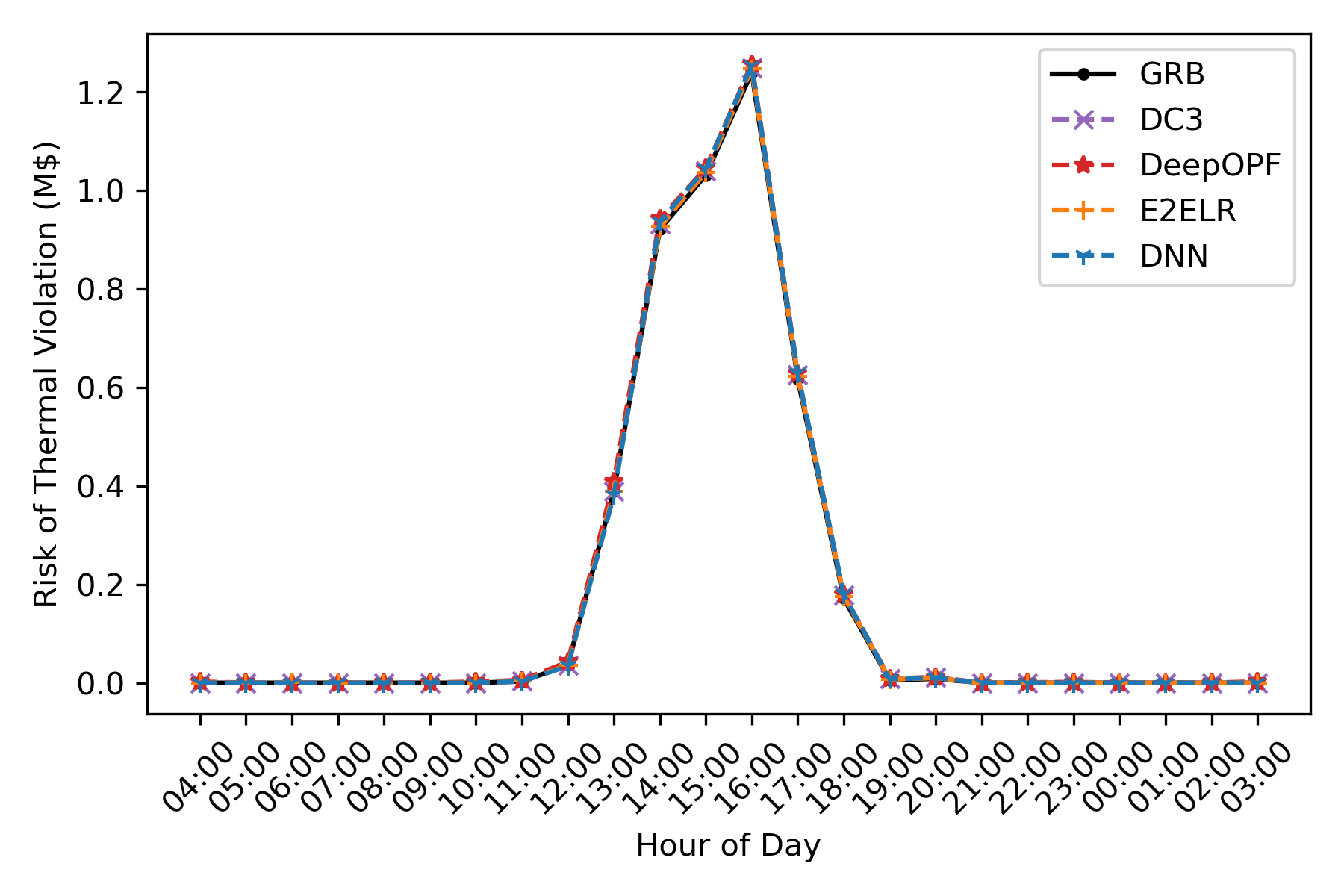
(c) Level-3 (financial risk) metrics for ieee300. Left: risk of system power imbalance, in log scale. Right: risk of total thermal violations.

Figure 4: Risk assessment results on the ieee300 system.

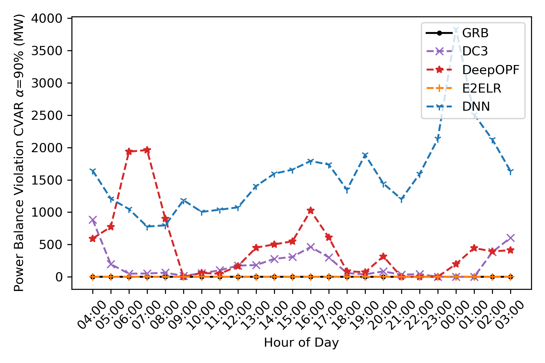
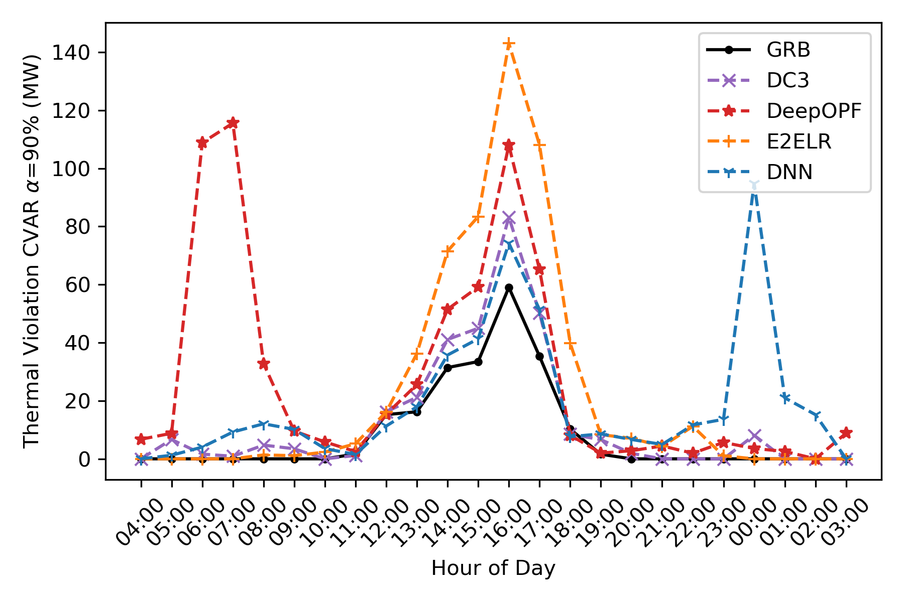
(a) Level-1 (CVaR) risk metrics for pegase1k. Left: $\text{CVaR}_{90\%}$ of system power imbalance. Right: $\text{CVaR}_{90\%}$ of total thermal violations.

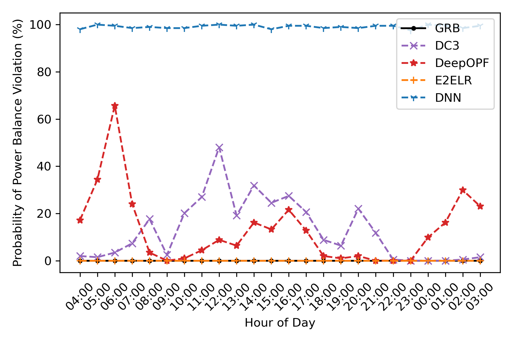
(b) Level-2 (probability of adverse event) risk metrics for pegase1k. Left: probability of system power imbalance. Right: probability of non-zero total thermal violations.

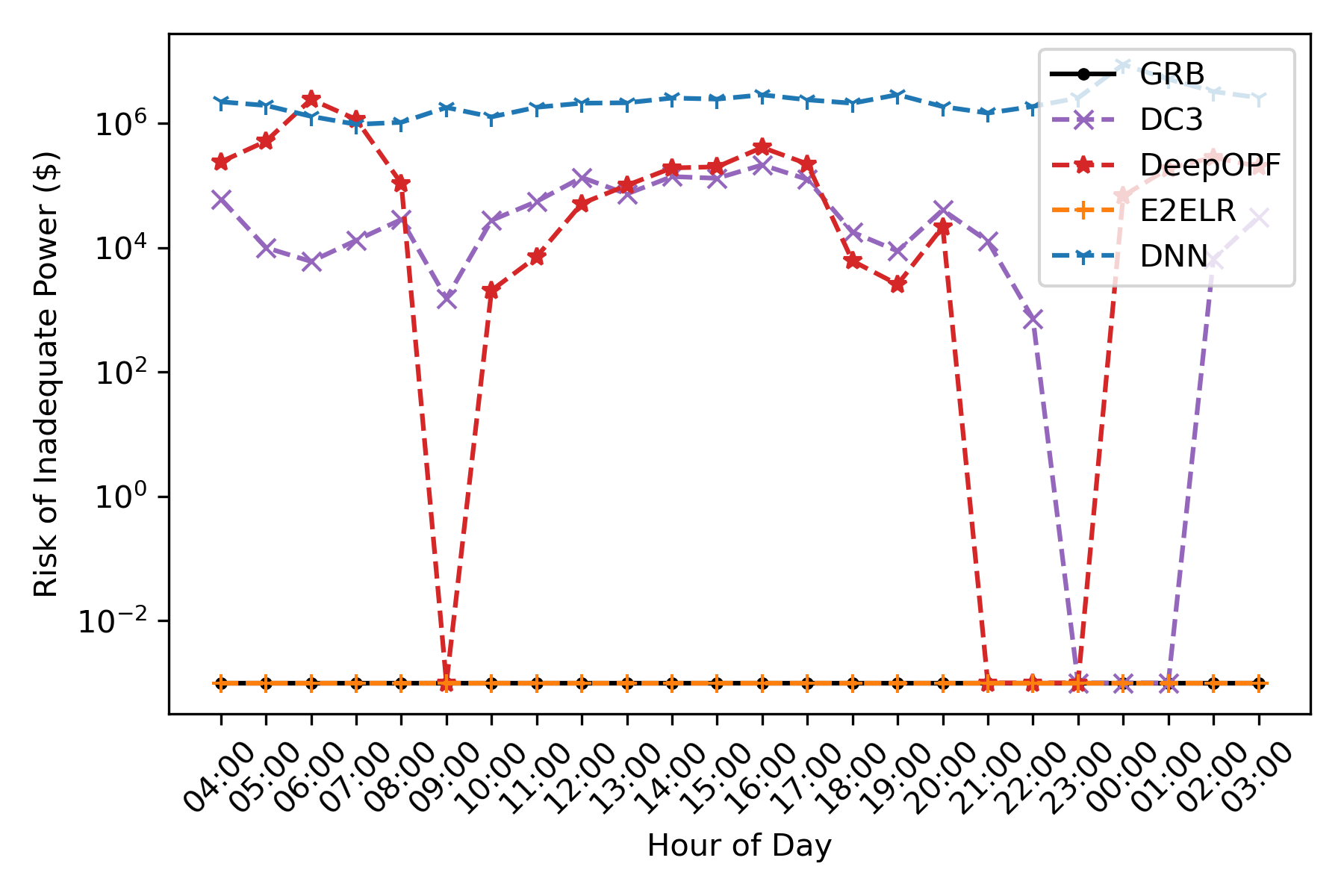
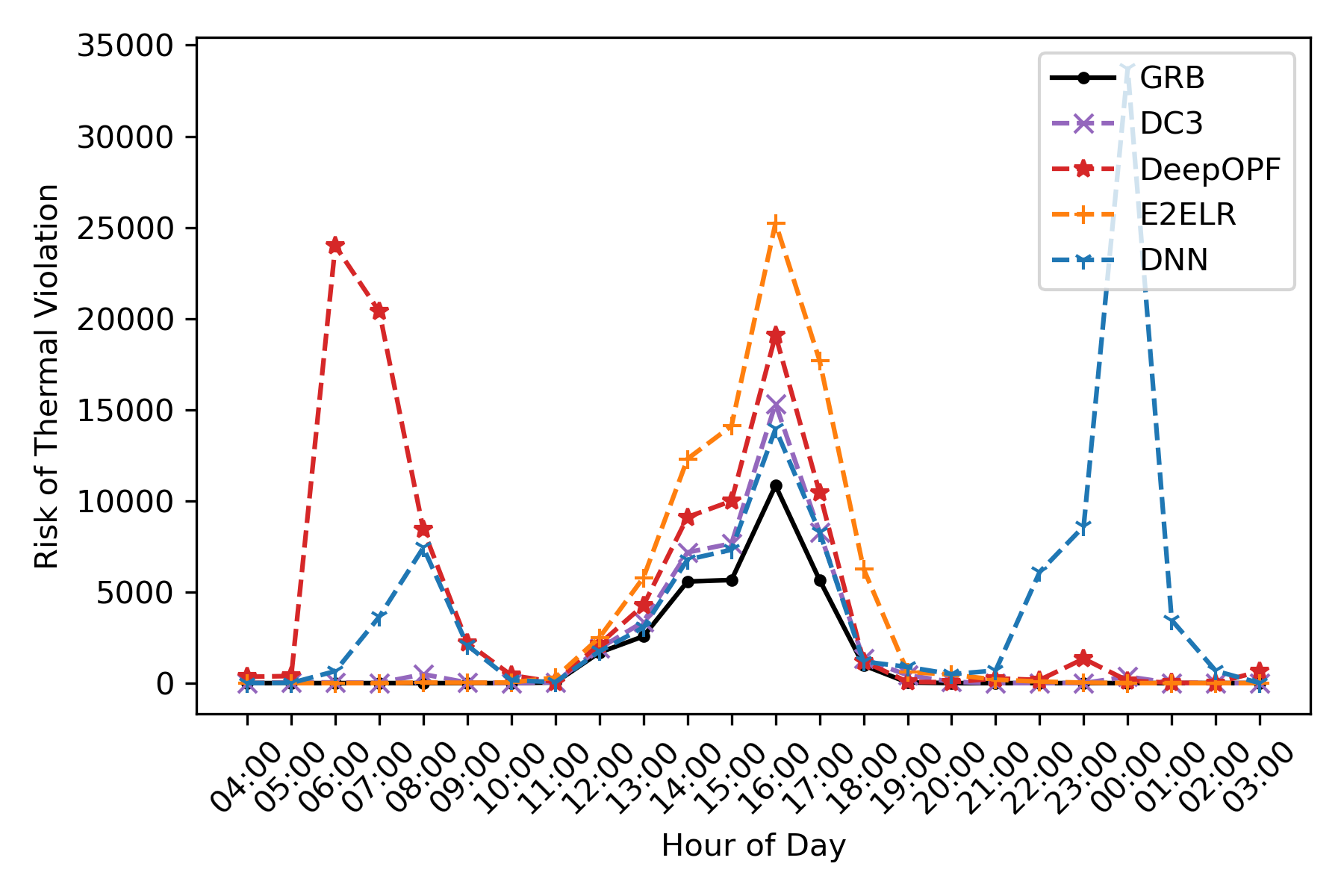
(c) Level-3 (financial risk) metrics for pegase1k. Left: risk of system power imbalance, in log scale. Right: risk of total thermal violations.

Figure 5: Risk assessment results on the pegase1k system.

First observe that RA-DNN, RA-DC3 and RA-DeepOPF consistently over-estimates power imbalances. This is most striking for RA-DNN, which almost always predicts non-zero power imbalances, while RA-DeepOPF and RA-DC3 wrongly predict system imbalances during the afternoon hours on ieee300 and throughout the day on pegase1k. This is because the DNN, DeepOPF, and DC3 are not guaranteed to output solutions that satisfy all ED constraints. In contrast, the E2ELR architecture, which always outputs ED-feasible solutions, prefectly matches the ground truth risk assessment for power imbalances.

Second, all proxies tend to over-estimate thermal violations, which is more flagrant on the larger pegase1k system (Figure 5). RA-DNN, RA-DeepOPF and, to a lesser extent, RA-DC3, incorrectly predict thermal violations during the morning hours (5am–9am) and during the night (10pm–2am). While the E2ELR-based risk profile over-estimates thermal violations during the afternoon (12pm–5pm), Figure 5b shows that RA-DC3 and RA-E2ELR correctly identify those hours during which congestion occurs. It is important to note that inaccurate risk predictions may result in unnecessary preventive actions, which result in higher economic cost for the system.

V-F Global Cost Analysis

In addition to operational risk, grid operators rely on accurate cost estimates to operate the grid as economically as possible. Therefore, Figure 6 depicts, for each proxy architecture, the hourly distribution of total costs for the pegase1k system. Here, total costs include generation costs, thermal violation costs, and power balance violation costs. Each figure displays the 2.5%, mean and 97.5% quantiles of ground truth cost distribution (in orange), and the cost distribution obtained by the proxy (in blue).

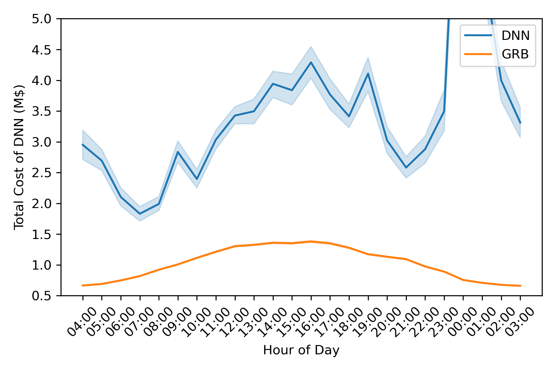
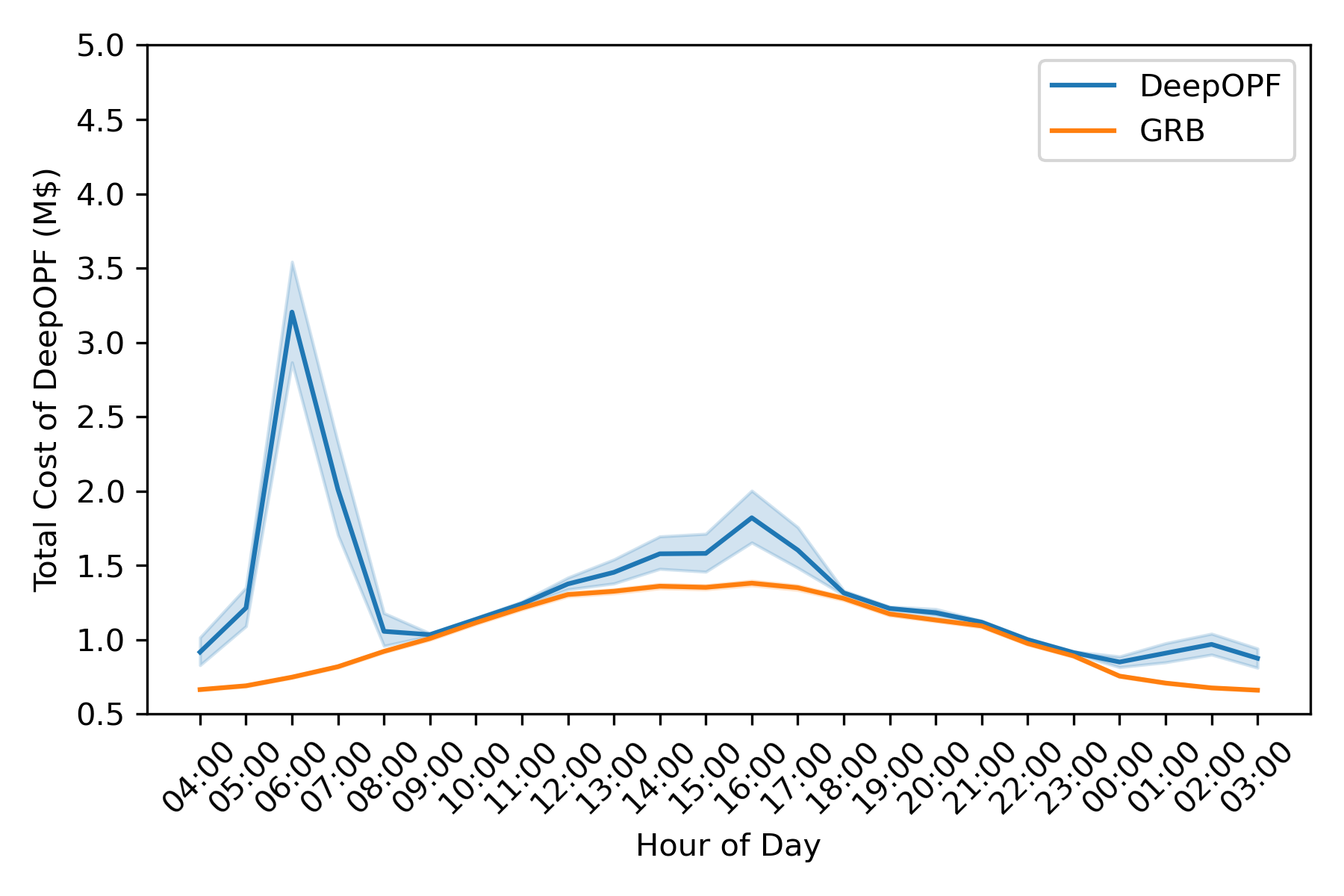
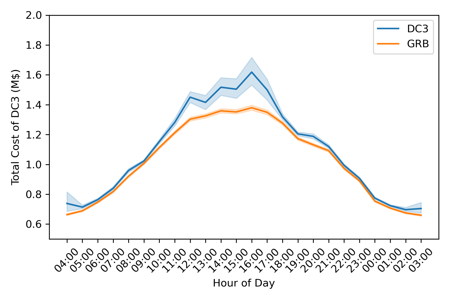
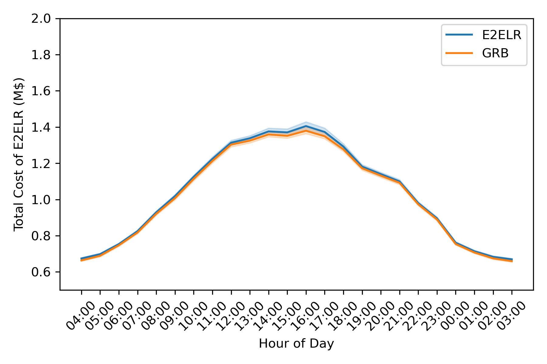
Figure 6: Hourly distributions of total cost on pegase1k: comparison between ground truth (GRB) and proxies. Top: RA-DNN (left) and RA-DeepOPF (right); Bottom: RA-DC3 (left) and RA-E2ELR (right). All values in M$.

First, throughout the entire day, RA-DNN significantly misestimates total costs. Similarly, RA-DeepOPF over-estimates costs costs, especially in the early morning (4am–8am), afternoon (2pm–5pm) and at night (12am–3am). Both of these are caused by incorrect predictions of system imbalance and thermal violations (see Figure 5). While RA-DC3 is more accurate, it still over-estimates total costs between 10am and 7pm, also mainly because of errors in power balance violations. The RA-E2ELR architecture achieves the best results, and almost perfectly matches the ground truth cost distribution.

To complement the above analysis, Figure 7 presents quantile-quantile (QQ) plots that compare, for both systems, the distribution of total costs (over the entire day) obtained by the ground truth optimization-based and proxy-based simulations. RA-DNN is omitted from the figure due to its poor performance. For ieee300, all proxies accurately capture the distribution of total costs. However, for pegase1k, RA-DeepOPF and RA-DC3 significantly deviate from the ground truth distribution: both architectures significantly over-estimate total costs for costlier (and riskier) scenarios. This is mostly due to incorrect predictions of system imbalances, which incur high penalty costs. In contrast, RA-E2ELR matches the ground truth distribution almost perfectly.

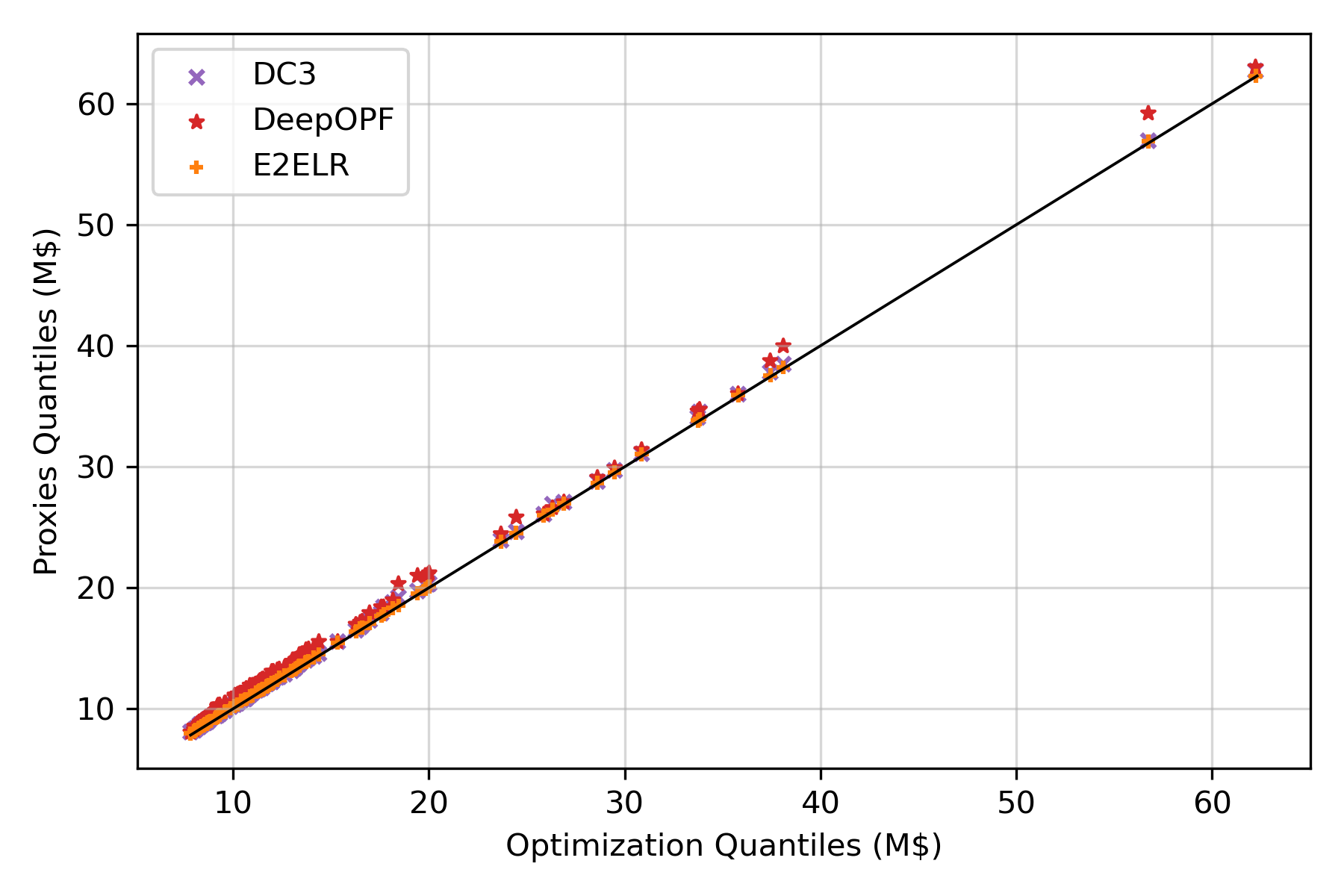
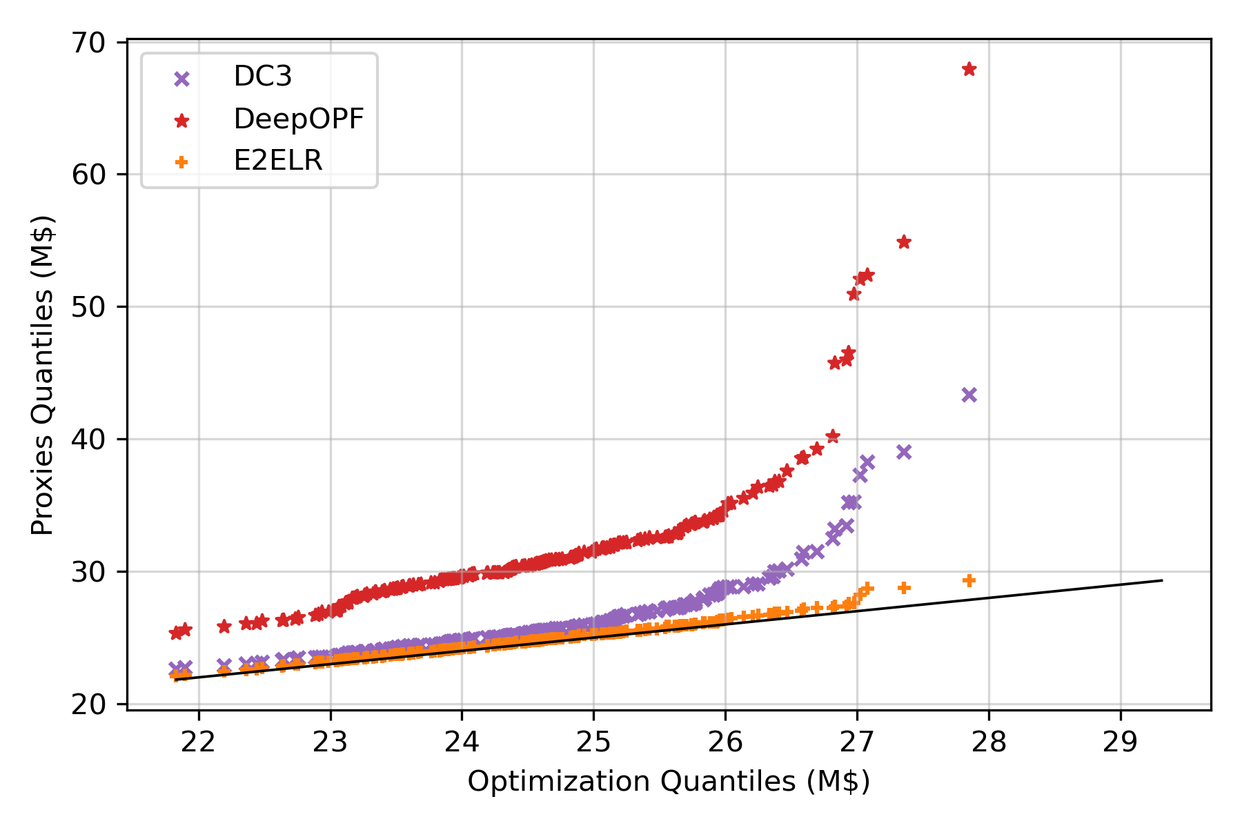
Figure 7: QQ plot of the total cost on 300 IEEE (left) and 1354 Pegase system (right). RA-DNN is omitted due to its poor performance.

V-G Component-level Risk Analysis

One of the advantages of the proposed proxy-based risk assessment frameworks is its granularity, i.e., it can produce risk profiles down to individual components. To demonstrate this capability, Figure 8 compares ground truth and proxy-based probability of thermal violations on each individual branch in ieee300 at 12pm, which is the hour with the most violations. Figure 8a displays the original grid, Figure 8b displays the ground truth result, and Figures 8c and 8d display the proxy-based results obtained with RA-DC3 and RA-E2ELR, respectively. The proxies correctly identify all branches with non-zero probability of thermal violations.

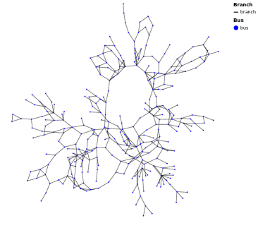
(a) The IEEE 300-bus system

(b) Branch-level probability of thermal violations (ground truth)

(c) Branch-level probability of thermal violation (RA-DC3)

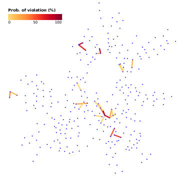
(d) Branch-level probability of thermal violation (RA-E2ELR)

Figure 8: Branch-level probability of thermal violations for the ieee300 system at 12pm.

V-H Computing Times

Table I compares computing times for proxy-based and optimization-based (GRB) risk assessment methods. Computing times for GRB scale roughly linearly with the size of the system, taking an average 0.5 and 2.2s per simulation per CPU core. Note that congested scenarios typically lead to increased computing times. In contrast, the simulation time of the proxies is consistent across different systems, typically taking less than 100 milliseconds to run 100 simulations. Specifically, RA-E2ELR achieves 30.3x speed up than GRB, even under the assumption that hundreds of ED instances can be solved in parallel. Among the proxies, RA-DC3 is the slowest because every inference requires 200 gradient steps.

TABLE I: Risk simulation computing times

Systems	E2ELR	DC3†	DeepOPF	DNN	GRB∗
ieee300	71.5	192.0	77.6	50.2	488.0
pegase1k	72.0	211.4	59.0	49.6	2188.0

All times in ms. ML inference times are per batch of 100 scenarios on 1 GPU. ^∗Average time per scenario using 1 CPU. ^†with 200 gradient steps.

VI Conclusion

The paper has presented the first risk-assessment framework for power systems, RA-E2ELR, that uses end-to-end feasible optimization proxies. The proposed framework leverages the speed of optimization proxies and the feasibility guarantees of the E2ELR architecture. Numerical experiments demonstrated that RA-E2ELR yields high-quality risk estimates, and a 30x speedup over optimization-based simulations. This contrasts with previously-proposed architectures like DeepOPF and DC3, which offer no significant speed advantage over E2ELR but whose lack of feasibility guarantees results in over-predicting risks and costs.

References

- [1] O. Stover, P. Karve, and S. Mahadevan, “Reliability and risk metrics to assess operational adequacy and flexibility of power grids,” Reliability Engineering & System Safety, vol. 231, p. 109018, 2023.
- [2] W. Chen, M. Tanneau, and P. V. Hentenryck, “End-to-End Feasible Optimization Proxies for Large-Scale Economic Dispatch,” IEEE Transactions on Power Systems, pp. 1–12, 2023.
- [3] A. A. Thatte and L. Xie, “A metric and market construct of inter-temporal flexibility in time-coupled economic dispatch,” IEEE Transactions on Power Systems, vol. 31, no. 5, pp. 3437–3446, 2015.
- [4] E. Lannoye, D. Flynn, and M. O’Malley, “Evaluation of power system flexibility,” IEEE Transactions on Power Systems, vol. 27, no. 2, pp. 922–931, 2012.
- [5] “North american electric reliability corporation. probabilistic adequacy and measures,” Technical reference report final,, 2018.
- [6] Y. Zhou, B. Zhang, C. Xu, T. Lan, R. Diao, D. Shi, Z. Wang, and W.-J. Lee, “A Data-Driven Method for fast AC Optimal Power Flow Solutions via Deep Reinforcement Learning,” Journal of Modern Power Systems and Clean Energy, vol. 8, no. 6, pp. 1128–1139, 2020.
- [7] Z. Yan and Y. Xu, “Real-time optimal power flow: A lagrangian based deep reinforcement learning approach,” IEEE Transactions on Power Systems, vol. 35, no. 4, pp. 3270–3273, 2020.
- [8] A. R. Sayed, C. Wang, H. Anis, and T. Bi, “Feasibility constrained online calculation for real-time optimal power flow: A convex constrained deep reinforcement learning approach,” IEEE Transactions on Power Systems, 2022.
- [9] A. R. Sayed, X. Zhang, G. Wang, C. Wang, and J. Qiu, “Optimal operable power flow: Sample-efficient holomorphic embedding-based reinforcement learning,” IEEE Transactions on Power Systems, 2023.
- [10] L. Zeng, M. Sun, X. Wan, Z. Zhang, R. Deng, and Y. Xu, “Physics-constrained vulnerability assessment of deep reinforcement learning-based scopf,” IEEE Transactions on Power Systems, 2022.
- [11] MISO, “Energy and operating reserve markets,” 2022, Business Practices Manual Energy and Operating Reserve Markets.
- [12] O. Stover, P. Karve, S. Mahadevan, W. Chen, H. Zhao, M. Tanneau, and P. Van Hentenryck, “Just-in-time learning for operational risk assessment in power grids,” arXiv preprint arXiv:2209.12762, 2022.
- [13] S. Park and P. Van Hentenryck, “Self-supervised primal-dual learning for constrained optimization,” in Proceedings of the AAAI Conference on Artificial Intelligence, vol. 37, no. 4, 2023, pp. 4052–4060.
- [14] X. Pan, T. Zhao, M. Chen, and S. Zhang, “Deepopf: A deep neural network approach for security-constrained dc optimal power flow,” IEEE Transactions on Power Systems, vol. 36, no. 3, pp. 1725–1735, 2020.
- [15] P. L. Donti, D. Rolnick, and J. Z. Kolter, “DC3: A learning method for optimization with hard constraints,” preprint arXiv:2104.12225, 2021.
- [16] University of Washington, Dept. of Electrical Engineering, “Power Systems Test Case Archive.” [Online]. Available: http://www.ee.washington.edu/research/pstca/
- [17] C. Josz, S. Fliscounakis, J. Maeght, and P. Panciatici, “AC Power Flow Data in MATPOWER and QCQP Format: iTesla, RTE Snapshots, and PEGASE,” 2016.
- [18] A. S. Xavier, A. M. Kazachkov, O. Yurdakul, and F. Qiu, “UnitCommitment.jl: A Julia/JuMP Optimization Package for Security-Constrained Unit Commitment,” Jul. 2022. [Online]. Available: https://doi.org/10.5281/zenodo.6857290
- [19] A. S. Xavier, F. Qiu, and S. Ahmed, “Learning to Solve Large-Scale Security-Constrained Unit Commitment Problems,” INFORMS Journal on Computing, vol. 33, no. 2, pp. 739–756, 2021.
- [20] I. Dunning, J. Huchette, and M. Lubin, “JuMP: A Modeling Language for Mathematical Optimization,” SIAM Review, vol. 59, no. 2, pp. 295–320, 2017.
- [21] Gurobi Optimization, LLC, “Gurobi Optimizer Reference Manual,” 2023. [Online]. Available: https://www.gurobi.com
- [22] A. Paszke, S. Gross, S. Chintala, G. Chanan, E. Yang, Z. DeVito, Z. Lin, A. Desmaison, L. Antiga, and A. Lerer, “Automatic differentiation in pytorch,” in NIPS-W, 2017.
- [23] D. P. Kingma and J. Ba, “Adam: A method for stochastic optimization,” in 3rd International Conference on Learning Representations, ICLR 2015, San Diego, CA, USA, May 7-9, 2015, Conference Track Proceedings, Y. Bengio and Y. LeCun, Eds., 2015.
- [24] PACE, Partnership for an Advanced Computing Environment (PACE), 2017. [Online]. Available: http://www.pace.gatech.edu