Abstract

Active Flux is an extension of the Finite Volume method and additionally incorporates point values located at cell boundaries. This gives rise to a globally continuous approximation of the solution. The method is third-order accurate. We demonstrate that a new semi-discrete Active Flux method (first described in [AB23a] for one space dimension) can easily be used to solve nonlinear hyperbolic systems in multiple dimensions, such as the compressible Euler equations of inviscid hydrodynamics. Originally, the Active Flux method emerged as a fully discrete method, and required an exact or approximate evolution operator for the point value update. For nonlinear problems such an operator is often difficult to obtain, in particular for multiple spatial dimensions. With the new approach it becomes possible to leave behind these difficulties. We introduce a multi-dimensional limiting strategy and demonstrate the performance of the new method on both Riemann problems and subsonic flows.

Keywords: Compressible Euler equations, Active Flux, High-order methods

Mathematics Subject Classification (2010): 65M08, 65M20, 65M70, 76M12

Rémi Abgrall, Wasilij Barsukow, Christian Klingenberg

1 Introduction

The Active Flux method uses as its degrees of freedom both cell averages and point values at cell interfaces. While the averages require a conservative update, the update of the point values is essentially not restricted by more than the condition that the resulting method should be stable. To this end it needs to incorporate upwinding, and the earliest version of the Active Flux method ([vL77], for linear advection in 1-d) traced a characteristic back to the time level $t^{n}$ where a reconstruction of the data was evaluated. This approach was extended in [Bar21] to nonlinear scalar conservation laws in multiple dimensions, and to hyperbolic systems of conservation laws in one spatial dimension. The exact calculation of the characteristic curve was replaced by a sufficiently accurate approximation. This approach was used, for example, in [BB23] to solve the shallow water equations in presence of dry areas.

For hyperbolic systems in multiple spatial dimensions, even if they are linear, characteristic curves no longer exist. Also, values in general are not transported, but the solution is a convolution of the initial data with a more or less complicated kernel. For the acoustic equations with the speed of sound $c$, for example, the solution in $x$ at time $t$ depends on the initial data in a disc with radius $ct$ around $x$. This disc is the interior of the intersection of the hypersurface of initial data with the cone of bicharacteristics which has its vertex at $(t,x)$. In [ER13], a solution operator was given for the acoustic equations, which relied on smoothness of the initial data, and in [BK22] a solution in the sense of distributions was obtained which could be used to solve e.g. Riemann problems. These operators can be implemented efficiently and used to update the point values in an Active Flux method (as achieved in [BHKR19]), but their derivation comes at great cost. Suitably high-order approximate evolution operators for multi-dimensional nonlinear systems of conservation laws are currently unavailable.

All these Active Flux methods were $3^{\text{rd}}$ order accurate and fully-discrete. In [Abg22], a semi-discrete version of Active Flux was introduced. In order to obtain an equation for the point values, the spatial derivative in the PDE is discretized using finite difference formulae. At the price of a slightly reduced CFL condition this approach is immediately applicable to all kinds of nonlinear problems. In [AB23a, AB23b] it has been applied to one-dimensional nonlinear problems, and extended to arbitrary order. The aim of the present work is, maintaining $3^{\text{rd}}$ order of accuracy, to extend it to the multi-dimensional Euler equations.

The paper is organized as follows: Section 2 describes the method and Section 3 presents a novel multi-dimensional limiting strategy. Numerical results are shown in Section 4.

2 The semi-discrete Active Flux method

Here, we let ourselves guide by the approach of [AB23a] and extend it to multi-dimensional Cartesian grids. Consider a hyperbolic $m\times m$ system of conservation laws in $d$ spatial dimensions

$$\partial_{t}q+\nabla\cdot\mathbf{f}(q) =0\qquad q\colon\mathbb{R}^{+}_{0}\times\mathbb{R}^{d}\to\mathbb{R}^{m}$$ (1)

For simplicity, we restrict ourselves to two spatial dimensions ($d=2$) and write $\mathbf{f}=(f^{x},f^{y})$, $\nabla_{q}f^{x}=J^{x}$, $\nabla_{q}f^{y}=J^{y}$.

2.1 Update of the averages

Integrating (1) over the Cartesian cell

$$C_{ij}:=\left[x_{i-\frac{1}{2}},x_{i+\frac{1}{2}}\right]\times\left[y_{j-\frac{1}{2}},y_{j+\frac{1}{2}}\right]$$ (2)

and denoting the cell average by

$$\bar{q}_{ij}(t):=\frac{1}{\Delta x\Delta y}\int_{C_{ij}}q(t,\mathbf{x})\mathrm{d}\mathbf{x}$$ (3)

one finds

$$\frac{\mathrm{d}}{\mathrm{d}t}\bar{q}_{ij}+\frac{1}{\Delta x\Delta y}\int_{\partial C_{ij}}\mathbf{n}\cdot\mathbf{f}(q) =0$$ (4)

As there are degrees of freedom located at the boundary $\partial C_{ij}$ of cell $C_{ij}$, we intend to use them as quadrature points for a sufficiently accurate quadrature of the integral appearing in (4). Inspired by previous approaches (e.g. [BHKR19, HKS19]) we use three Gauss-Lobatto points per edge, where the extreme points (corners) are shared. Note also that we enforce global continuity: the point values on an edge are the same as seen from either of the adjacent cells and a value at a corner is involved in the update of four cells. This is in contrast to e.g. discontinuous Galerkin methods.

On Cartesian grids it is convenient to adopt the following notation for the 8 point values on the boundary of cell $C_{ij}$:

$$q_{i-\frac{1}{2},j+\frac{1}{2}} q_{i,j+\frac{1}{2}} q_{i+\frac{1}{2},j+\frac{1}{2}}$$

$$q_{i-\frac{1}{2},j} q_{i+\frac{1}{2},j}$$

$$q_{i-\frac{1}{2},j-\frac{1}{2}} q_{i,j-\frac{1}{2}} q_{i+\frac{1}{2},j-\frac{1}{2}}$$

Then,

$$\frac{\mathrm{d}}{\mathrm{d}t}\bar{q}_{ij} +\frac{1}{\Delta x\Delta y}\int_{y_{j-\frac{1}{2}}}^{y_{j+\frac{1}{2}}}\mathrm{d}y\Big{(}f^{x}(q(t,x_{i+\frac{1}{2}},y))-f^{x}(q(t,x_{i-\frac{1}{2}},y))\Big{)}$$ (5)

$$+\frac{1}{\Delta x\Delta y}\int_{x_{i-\frac{1}{2}}}^{x_{i+\frac{1}{2}}}\mathrm{d}x\Big{(}f^{y}(q(t,x,y_{j+\frac{1}{2}})-f^{y}(q(t,x,y_{j-\frac{1}{2}})\Big{)}=0$$ (6)

using Simpson’s rule ($\omega_{-\frac{1}{2}}=\omega_{\frac{1}{2}}=\frac{1}{6}$, $\omega_{0}=\frac{2}{3}$) becomes

$$\frac{\mathrm{d}}{\mathrm{d}t}\bar{q}_{ij}(t) +\frac{1}{\Delta x}\sum_{K=-\frac{1}{2},0,\frac{1}{2}}\omega_{K}\left(f^{x}(q_{i+\frac{1}{2},j+K}(t))-f^{x}(q_{i-\frac{1}{2},j+K}(t))\right)$$ (7)

$$+\frac{1}{\Delta y}\sum_{K=-\frac{1}{2},0,\frac{1}{2}}\omega_{K}\left(f^{y}(q_{i+K,j+\frac{1}{2}}(t))-f^{y}(q_{i+K,j-\frac{1}{2}}(t))\right)=0$$ (8)

This method is conservative, with e.g. the $x$-flux through the cell interface $(i+\frac{1}{2},j)$ being given by

$$\hat{f}^{x}_{i+\frac{1}{2},j} =\sum_{K=-\frac{1}{2},0,\frac{1}{2}}\omega_{K}f^{x}(q_{i+\frac{1}{2},j+K})$$ (9)

$$=\frac{f^{x}(q_{i+\frac{1}{2},j-\frac{1}{2}})+4f^{x}(q_{i+\frac{1}{2},j})+f^{x}(q_{i+\frac{1}{2},j+\frac{1}{2}})}{6}$$ (10)

It is also at least $3^{\text{rd}}$ order accurate, for it is exact for biparabolic functions.

2.2 Update of the point values

The update of the cell averages, as described above, now needs to be complemented by an update of the point values. In the one-dimensional case, it was proposed in [AB23a] to replace the spatial derivatives appearing in (1) by finite differences. Here, the multi-dimensional case shall be addressed. Note first that hyperbolicity of (1) implies that it is always possible to define the positive and negative parts of the Jacobians via their eigenvalues. With $J^{x}=R\mathrm{diag}(\lambda_{1},\ldots,\lambda_{m})R^{-1}$ one has

$$(J^{x})^{+} :=R\mathrm{diag}(\lambda_{1}^{+},\ldots,\lambda_{m}^{+})R^{-1}$$ (11)

$$(J^{x})^{+} :=R\mathrm{diag}(\lambda_{1}^{-},\ldots,\lambda_{m}^{-})R^{-1}$$ (12)

where, for scalars $a\in\mathbb{R}$ the positive/negative parts are simply $a^{+}=\max(0,a)$, $a^{-}=\min(0,a)$.

The finite difference formulae are obtained by differentiating a reconstruction. Define first the unique biparabolic polynomial

$$q_{ij,\text{recon}}\in P^{2,2},\quad q_{ij,\text{recon}}\colon\left[-\frac{\Delta x}{2},\frac{\Delta x}{2}\right]\times\left[-\frac{\Delta y}{2},\frac{\Delta y}{2}\right]\to\mathbb{R}^{m}$$ (13)

that interpolates the degrees of freedom of cell $ij$:

$$q_{ij,\text{recon}}\left(-\frac{\Delta x}{2},\frac{\Delta y}{2}\right) =q_{i-\frac{1}{2},j+\frac{1}{2}} q_{ij,\text{recon}}\left(0,\frac{\Delta y}{2}\right) =q_{i,j+\frac{1}{2}}$$

$$q_{ij,\text{recon}}\left(\frac{\Delta x}{2},\frac{\Delta y}{2}\right) =q_{i+\frac{1}{2},j+\frac{1}{2}}$$

$$q_{ij,\text{recon}}\left(-\frac{\Delta x}{2},0\right) =q_{i-\frac{1}{2},j} q_{ij,\text{recon}}\left(\frac{\Delta x}{2},0\right) =q_{i+\frac{1}{2},j}$$

$$q_{ij,\text{recon}}\left(-\frac{\Delta x}{2},-\frac{\Delta y}{2}\right) =q_{i-\frac{1}{2},j-\frac{1}{2}} q_{ij,\text{recon}}\left(0,-\frac{\Delta y}{2}\right) =q_{i,j-\frac{1}{2}}$$

$$q_{ij,\text{recon}}\left(\frac{\Delta x}{2},-\frac{\Delta y}{2}\right) =q_{i+\frac{1}{2},j-\frac{1}{2}}$$

and

$$\frac{1}{\Delta x\Delta y}\int_{-\frac{\Delta x}{2}}^{\frac{\Delta x}{2}}\int_{-\frac{\Delta y}{2}}^{\frac{\Delta y}{2}}q_{ij,\text{recon}}(x,y)\,\mathrm{d}y\mathrm{d}x =\bar{q}_{ij}$$ (14)

This reconstruction has already been used in [BHKR19, HKS19] and is given there explicitly. Then we define the finite differences in the corner as

$$(D^{x})^{+}_{i+\frac{1}{2},j+\frac{1}{2}}q :=\partial_{x}q_{ij,\text{recon}}\left.\left(x,\frac{\Delta y}{2}\right)\right|_{x=\frac{\Delta x}{2}}$$ (15)

$$(D^{x})^{-}_{i+\frac{1}{2},j+\frac{1}{2}}q :=\partial_{x}q_{i+1,j,\text{recon}}\left.\left(x,\frac{\Delta y}{2}\right)\right|_{x=-\frac{\Delta x}{2}}$$ (16)

$$(D^{y})^{+}_{i+\frac{1}{2},j+\frac{1}{2}}q :=\partial_{y}q_{ij,\text{recon}}\left.\left(\frac{\Delta x}{2},y\right)\right|_{y=\frac{\Delta y}{2}}$$ (17)

$$(D^{y})^{-}_{i+\frac{1}{2},j+\frac{1}{2}}q :=\partial_{y}q_{i,j+1,\text{recon}}\left.\left(\frac{\Delta x}{2},y\right)\right|_{x=-\frac{\Delta y}{2}}$$ (18)

Observe that due to continuity,

$$(D^{x})^{+}_{i+\frac{1}{2},j+\frac{1}{2}}q =\partial_{x}q_{i,j+1,\text{recon}}\left(x,-\frac{\Delta y}{2}\right)\Big{|}_{x=\frac{\Delta x}{2}}$$ (19)

such that this would be an equivalent definition that gives the same result (and similarly for the other finite differences). Analogously, we define the finite differences on the edges

$$(D^{x})^{+}_{i+\frac{1}{2},j}q :=\partial_{x}q_{ij,\text{recon}}\left.\left(x,0\right)\right|_{x=\frac{\Delta x}{2}}$$ (20)

$$(D^{x})^{-}_{i+\frac{1}{2},j}q :=\partial_{x}q_{i+1,j,\text{recon}}\left.\left(x,0\right)\right|_{x=-\frac{\Delta x}{2}}$$ (21)

$$(D^{y})_{i+\frac{1}{2},j}q :=\partial_{x}q_{ij,\text{recon}}\left.\left(\frac{\Delta x}{2},y\right)\right|_{y=0}$$ (22)

Observe that due to continuity, there is no distinction between $(D^{y})^{+}_{i+\frac{1}{2},j}$ and $(D^{y})^{-}_{i+\frac{1}{2},j}$. Here, again, the symmetric definition

$$(D^{y})_{i+\frac{1}{2},j}q :=\partial_{y}q_{i+1,j,\text{recon}}\left.\left(-\frac{\Delta x}{2},y\right)\right|_{y=0}$$ (23)

yields the same result. The derivatives at $(i,j+\frac{1}{2})$ are obtained analogously. For reference we now state their explicit forms:

$$\left(D^{x}\right)^{+}_{i+\frac{1}{2},j}q =\frac{1}{4\Delta x}\left(4\left(-9\bar{q}_{ij}+2\left(q_{i-\frac{1}{2},j}+2q_{i+\frac{1}{2},j}\right)\right)+4\left(q_{i,j-\frac{1}{2}}+q_{i,j+\frac{1}{2}}\right)\right.$$

$$\left.+q_{i-\frac{1}{2},j-\frac{1}{2}}+q_{i+\frac{1}{2},j-\frac{1}{2}}+q_{i-\frac{1}{2},j+\frac{1}{2}}+q_{i+\frac{1}{2},j+\frac{1}{2}}\right)$$

$$\left(D^{x}\right)^{-}_{i+\frac{1}{2},j}q =-\frac{1}{4\Delta x}\left(-36\bar{q}_{i+1,j}+8\left(2q_{i+\frac{1}{2},j}+q_{i+\frac{3}{2},j}\right)+q_{i+\frac{1}{2},j-\frac{1}{2}}\right.$$

$$\left.+4\left(q_{i+1,j-\frac{1}{2}}+q_{i+1,j+\frac{1}{2}}\right)+q_{i+\frac{3}{2},j-\frac{1}{2}}+q_{i+\frac{1}{2},j+\frac{1}{2}}+q_{i+\frac{3}{2},j+\frac{1}{2}}\right)$$

$$\left(D^{y}\right)_{i+\frac{1}{2},j}q =\frac{q_{i+\frac{1}{2},j+\frac{1}{2}}-q_{i+\frac{1}{2},j-\frac{1}{2}}}{\Delta y}$$

$$\left(D^{y}\right)^{+}_{i,j+\frac{1}{2}}q =\frac{1}{4\Delta y}\left(4\left(q_{i-\frac{1}{2},j}-9\bar{q}_{ij}+q_{i+\frac{1}{2},j}\right)+q_{i-\frac{1}{2},j-\frac{1}{2}}+q_{i-\frac{1}{2},j+\frac{1}{2}}\right.$$

$$\left.+q_{i+\frac{1}{2},j-\frac{1}{2}}+q_{i+\frac{1}{2},j+\frac{1}{2}}+8\left(q_{i,j-\frac{1}{2}}+2q_{i,j+\frac{1}{2}}\right)\right)$$

$$\left(D^{y}\right)^{-}_{i,j+\frac{1}{2}}q =-\frac{1}{4\Delta y}\left(4\left(q_{i-\frac{1}{2},j+1}-9\bar{q}_{i,j+1}+q_{i+\frac{1}{2},j+1}\right)+q_{i-\frac{1}{2},j+\frac{1}{2}}\right.$$

$$\left.+q_{i+\frac{1}{2},j+\frac{1}{2}}+q_{i-\frac{1}{2},j+\frac{3}{2}}+q_{i+\frac{1}{2},j+\frac{3}{2}}+8\left(2q_{i,j+\frac{1}{2}}+q_{i,j+\frac{3}{2}}\right)\right)$$

$$\left(D^{x}\right)_{i,j+\frac{1}{2}}q =\frac{q_{i+\frac{1}{2},j+\frac{1}{2}}-q_{i-\frac{1}{2},j+\frac{1}{2}}}{\Delta x}$$

$$\left(D^{x}\right)^{+}_{i+\frac{1}{2},j+\frac{1}{2}}q =\frac{q_{i-\frac{1}{2},j+\frac{1}{2}}-4q_{i,j+\frac{1}{2}}+3q_{i+\frac{1}{2},j+\frac{1}{2}}}{\Delta x}$$

$$\left(D^{x}\right)^{-}_{i+\frac{1}{2},j+\frac{1}{2}}q =\frac{4q_{i+1,j+\frac{1}{2}}-3q_{i+\frac{1}{2},j+\frac{1}{2}}-q_{i+\frac{3}{2},j+\frac{1}{2}}}{\Delta x}$$

$$\left(D^{y}\right)^{+}_{i+\frac{1}{2},j+\frac{1}{2}}q =\frac{q_{i+\frac{1}{2},j-\frac{1}{2}}-4q_{i+\frac{1}{2},j}+3q_{i+\frac{1}{2},j+\frac{1}{2}}}{\Delta y}$$

$$\left(D^{y}\right)^{-}_{i+\frac{1}{2},j+\frac{1}{2}}q =\frac{4q_{i+\frac{1}{2},j+1}-3q_{i+\frac{1}{2},j+\frac{1}{2}}-q_{i+\frac{1}{2},j+\frac{3}{2}}}{\Delta y}$$

However, in some situations one might be willing to employ a different reconstruction, as is, for instance, the case in Section 3 concerned with limiting. At this point one has to resort to the more general formulae (15)–(22).

Finally, the upwinding is defined as

$$(J^{x}D^{x}_{i+K,j+L})^{\text{upw}}q:=(J^{x})^{+}(D^{x})^{+}_{i+K,j+L}q+(J^{x})^{-}(D^{x})^{-}_{i+K,j+L}q$$ (24)

with $K,L\in\{-\frac{1}{2},0,\frac{1}{2}\}$ and an analogous definition for $J^{y}$.

We propose to update the point values as follows:

$$\frac{\mathrm{d}}{\mathrm{d}t}q_{i+\frac{1}{2},j}+(J^{x}D^{x}_{i+\frac{1}{2},j})^{\text{upw}}q+J^{y}D^{y}_{i+\frac{1}{2},j}q =0$$ (25)

$$\frac{\mathrm{d}}{\mathrm{d}t}q_{i,j+\frac{1}{2}}+J^{x}D^{x}_{i,j+\frac{1}{2}}q+(J^{y}D^{y}_{i,j+\frac{1}{2}})^{\text{upw}}q =0$$ (26)

$$\frac{\mathrm{d}}{\mathrm{d}t}q_{i+\frac{1}{2},j+\frac{1}{2}}+(J^{x}D^{x}_{i+\frac{1}{2},j+\frac{1}{2}})^{\text{upw}}q+(J^{y}D^{y}_{i+\frac{1}{2},j+\frac{1}{2}})^{\text{upw}}q =0$$ (27)

As the finite differences are exact for biparabolic function, one expects $3^{\text{rd}}$ order of accuracy.

The complete method consists of the ODEs (8) (average update), (25)–(26) (point values at edge midpoints) and (27) (point values at nodes). We propose to integrate these with an SSP-RK3 method. In [AB23b], it was shown for the one-dimensional case that this approach leads to a stable scheme with a maximum CFL number of 0.41.

3 Limiting

Existing approaches to limiting in the context of standard Finite Volume methods modify the values of the reconstruction at a cell interface. They cannot be used for Active Flux due to its global continuity and the fact that point values at cell interfaces are prescribed and cannot be modified arbitrarily. Limiting employed in [HKS19] therefore gives up on continuity. Approaches to limiting that maintain continuity so far have only been treating the situation in which a parabolic reconstruction of monotone discrete data (point values and average) is not monotone, i.e. has an artificial extremum. In [RLM15], a piecewise linear/parabolic reconstruction is used in this case, and in [Bar21] the same situation is handled by replacing the parabola by a power law. One can show that then the reconstruction is always monotone whenever the discrete data are. Such modified reconstructions are effective in drastically reducing spurious oscillations, but they do not guarantee to remove them entirely. This is because the update of the averages is not limited and can itself create artificial extrema in the discrete data. However, in absence of better approaches, e.g. the power-law reconstruction is a viable limiting strategy. In particular, it is not computationally intensive.

In multiple spatial dimensions, a similar strategy is presented here for the first time. The multi-dimensional case is, however, much more complex because every cell has access to 8 point values. Consider point values at edge centers $q_{\text{N}},q_{\text{S}},q_{\text{W}},q_{\text{E}}$ and at vertices $q_{\text{NE}},q_{\text{SE}},q_{\text{NW}},q_{\text{SW}}$ of a (reference) Cartesian cell $c=[-\frac{\Delta x}{2},\frac{\Delta x}{2}]\times[-\frac{\Delta y}{2},\frac{\Delta y}{2}]$ and a cell average $\bar{q}$ to be given. We shall refer to the four edges as N-edge, S-edge, W-edge and E-edge, respectively. The reconstruction shall simply be denoted by $q_{\text{recon}}\colon c\to\mathbb{R}$ for simplicity. There exist two types of maximum-principle violation, which can occur independently of each other:

1. It can happen that the parabolic reconstruction along an edge (as part of a biparabolic reconstruction in the cell) overshoots/undershoots the three point values along the edge in question. For the example of an N-edge, this happens if either

   • the point values $q_{\text{NW}}$, $q_{\text{N}}$, $q_{\text{NE}}$ are not monotone and $q_{\text{NW}}\neq q_{\text{NE}}$, or if

   • they are monotone (i.e. either $q_{\text{NW}}<q_{\text{N}}<q_{\text{NE}}$ or $q_{\text{NW}}>q_{\text{N}}>q_{\text{NE}}$), but

     $$\left|q_{\text{N}}-\frac{q_{\text{NE}}+q_{\text{NW}}}{2}\right|>\frac{|q_{\text{NE}}-q_{\text{NW}}|}{4}$$ (28)

     such that the parabolic reconstruction has an artificial extremum.

   In this case the reconstruction along the edge shall be chosen continuous piecewise linear (“hat”). We shall say that the reconstruction along the edge is limited, or just that the “edge is limited”. To ensure continuity, the reconstruction in any cell with a limited edge can then no longer be biparabolic, but needs to be modified as detailed below and in Section A.1.

2. Define

   $$m:=\min(q_{\text{N}},q_{\text{S}},q_{\text{W}},q_{\text{E}},q_{\text{NE}},q_{\text{SE}},q_{\text{NW}},q_{\text{SW}})$$ (29)

   $$M:=\max(q_{\text{N}},q_{\text{S}},q_{\text{W}},q_{\text{E}},q_{\text{NE}},q_{\text{SE}},q_{\text{NW}},q_{\text{SW}})$$ (30)

   It can happen that despite

   $$m<\bar{q}<M$$ (31)

   the reconstruction $q_{\text{recon}}$ inside the cell $c$ fails to fulfill the maximum-principle, i.e.

   $$\exists x\in c\text{ such that either }q_{\text{recon}}(x)<m\text{ or }q_{\text{recon}}(x)>M$$ (32)

   This situation shall be improved by introducing a piecewise defined reconstruction with a central region where the function is constant (“plateau”), and connecting the plateau to the (parabolic or hat) reconstructions along the edges in a continuous fashion. More details are given below and in Section A.2; Figures 1 and 2 show examples. This new reconstruction fulfills

   $$m<q_{\text{recon}}(x)<M\qquad\forall x\in c$$ (33)

   We shall say that the reconstruction inside the cell is limited, or just that the “cell is limited”.

   This situation appears already in 1-d, in which case it has been suggested in [Bar21] to replace the parabolic reconstruction in the cell by a power law. A multi-dimensional analogue of the power law seems unfeasible, though, and we resort here to a piecewise defined, but easier function.

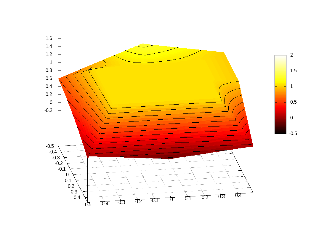
Figure 1: Left: An example of a plateau reconstruction. Here, $q_{\text{NW}}=1$, $q_{\text{W}}=1.35$, $q_{\text{SW}}=0.6$, $q_{\text{S}}=0.4$, $q_{\text{SE}}=0$, $q_{\text{E}}=-0.2$, $q_{\text{NE}}=0.0$, $q_{\text{N}}=1$, $\bar{q}=0.9$ (the S-edge is on the left). All edges but the S-edge are reconstructed as hats, the S-edge is reconstructed parabolically. Right: A piecewise-biparabolic reconstruction of the same data; one clearly observes an overshoot. The isolines have a spacing of 0.1.

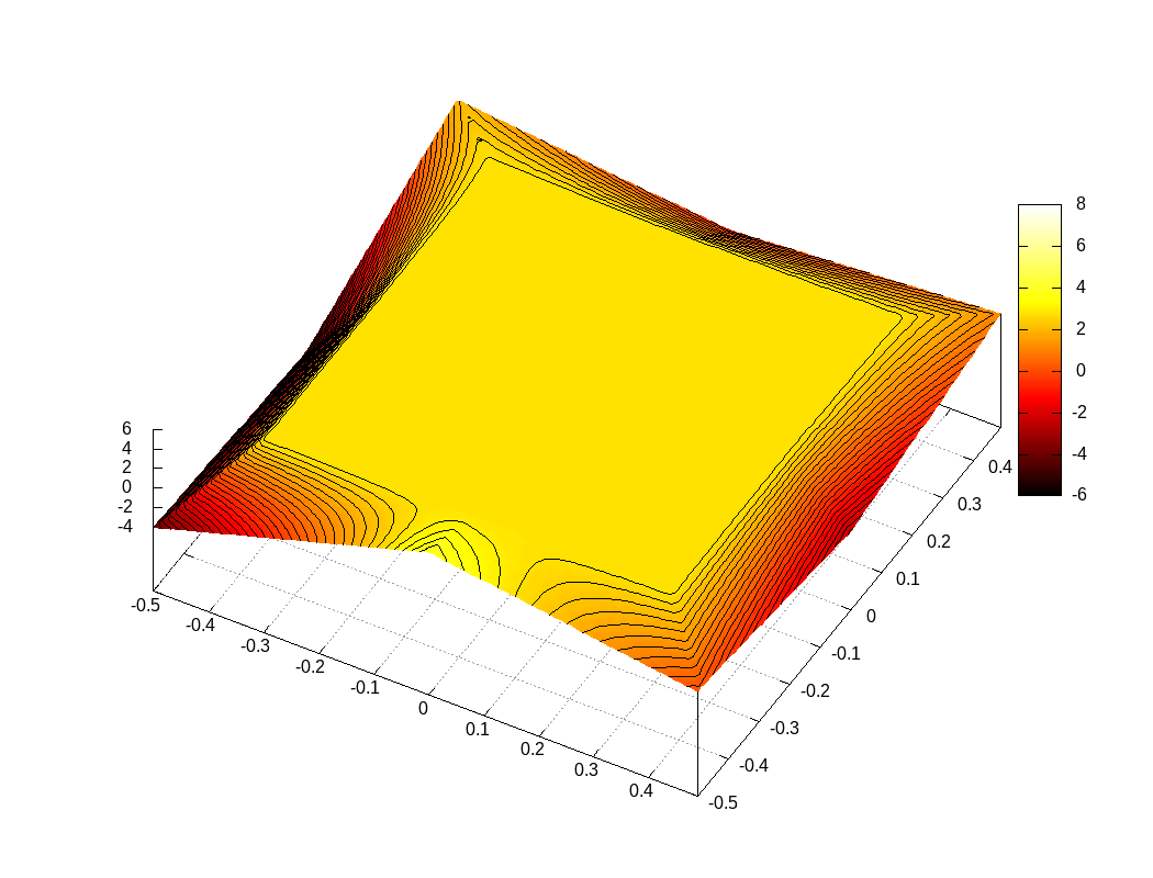
Figure 2: Left: An example of a plateau reconstruction. $q_{\text{NE}}=1,q_{\text{NW}}=2,q_{\text{SW}}=-4,q_{\text{SE}}=0,q_{\text{N}}=-1,q_{\text{S}}=4,q_{\text{W}}=-5,q_{\text{E}}=-3,\bar{q}=2$ (the W-edge is on the left). All edges are reconstructed as hats. Right: A piecewise-biparabolic reconstruction of the same data; one clearly observes an overshoot. The isolines have a spacing of 0.25.

The two situations are independent: any number of edges along the boundary of a cell might require limiting, and this will not generally imply anything about whether the cell itself is to be limited. The possible presence of hat functions along the boundary requires the reconstruction inside the cell to flexibly adapt to the different combinations of edge-reconstructions in order to be continuous. For instance, the plateau reconstruction needs to connect the plateau continuously to either a parabola, or a hat function (see Section A.2). Also, if there exists at least one edge that is reconstructed as a hat function, then one cannot use a biparabolic reconstruction inside the cell any longer, whether the cell is limited or not. Here, if the cell is not limited, but at least one edge, a piecewise-biparabolic reconstruction shall be used, detailed in Section A.1.

As we are aiming at a globally continuous reconstruction, that is computed locally from merely the cell average and the point values of the cell, the reconstruction along an edge can only depend on the three values associated to this edge, and cannot depend on other values in the cell. Indeed, if edge-reconstruction of one of edges of $c$ were to depend on, say, the average in the cell $c$, then the reconstruction in the neighbouring cell $c^{\prime}$ would also need to know about the average in $c$.

Due to the particular choice of degrees of freedom for Active Flux the reconstruction has to fulfill two types of conditions: It is supposed to interpolate the point values at cell interfaces and its average is supposed to be equal to the given one. The latter condition – merely to simplify the calculations – shall be replaced by a (yet unknown) point value $q_{\text{C}}$ at cell center which is kept as a variable in the formulae. Once the type of reconstruction in all regions of the cell has been determined, their integrals over the respective domains of definition can easily be found as functions of $q_{\text{C}}$, and $q_{\text{C}}$ is then determined by imposing the average of the reconstruction over the entire cell. This is a linear equation in $q_{\text{C}}$ due to linearity of the interpolation problem which makes $q_{\text{C}}$ enter linearly everywhere. The explicit formulae below therefore also depend on $q_{\text{C}}$, but the reconstruction in a cell in the end only depends on the point values along its boundary and on its average. This detour does not change the result but simplifies the algorithm.

The overall structure of the reconstruction algorithm is:

1. Decide for every edge of the cell whether it is reconstructed parabolically, or as a hat function.

2. Assume as hypothesis that the cell does not require limiting (i.e. that it is reconstructed in a piecewise biparabolic fashion) and compute the value of $q_{\text{C}}$ that ensures that the average of the reconstruction agrees with the given cell average.

3. Check (31) and if true, decide whether the piecewise-biparabolic reconstruction obtained in 2 violates the maximum principle

4. If this is the case, the cell needs to be limited with a plateau reconstruction. Compute the parameters $\eta,q_{\text{p}}$ (see below) of the plateau reconstruction that ensure maximum principle preservation and the correct value of the average of the reconstruction.

A pedagogical derivation of the reconstruction algorithm is given in Section A. Here, we only state all the relevant results in a concise way.

Theorem 3.1.

The following reconstruction $q_{\text{recon}}\colon\left[-\frac{\Delta x}{2},\frac{\Delta x}{2}\right]\times\left[-\frac{\Delta y}{2},\frac{\Delta y}{2}\right]\to\mathbb{R}$ is continuous, interpolates all the point values along the boundary of the cell, its average agrees with the given cell average and the reconstruction has the following properties:

1. If Condition (31), i.e. $m<\bar{q}<M$ is fulfilled, then $m\leq q_{\text{recon}}(x)\leq M$ for all $x$ inside the cell.

2. If $q_{\text{NW}}<q_{\text{N}}<q_{\text{NE}}$, then $q_{\text{NW}}\leq q_{\text{recon}}(x)\leq q_{\text{NE}}$ for all $x$ along the N-edge, and similarly for all the other edges.

The definition of the reconstruction is as follows: If $m<\bar{q}<M$ is not fulfilled, or if additionally $m<q^{\text{pw. biparab.}}_{\text{recon}}(x,y)<M$ for all $(x,y)\in c$, then

$$q_{\text{recon}}(x,y):=q^{\text{pw. biparab.}}_{\text{recon}}(x,y)$$ (34)

otherwise

$$q_{\text{recon}}(x,y):=q^{\text{plateau}}_{\text{recon}}(x,y),$$ (35)

the two types of reconstruction being defined as follows:

$$q_{\text{recon}}^{\text{pw. biparab.}}(x,y) :=q_{\text{recon}}^{\text{W}}\left(\frac{q_{\text{SW}}}{2},q_{\text{W}},\frac{q_{\text{NW}}}{2},x,y,\text{S},\text{N},\text{W},\frac{\Delta\bar{q}}{4}\right)$$ (36)

$$+q_{\text{recon}}^{\text{S}}\left(\frac{q_{\text{SE}}}{2},q_{\text{S}},\frac{q_{\text{SW}}}{2},x,y,\text{E},\text{W},\text{S},\frac{\Delta\bar{q}}{4}\right)$$

$$+q_{\text{recon}}^{\text{N}}\left(\frac{q_{\text{NW}}}{2},q_{\text{N}},\frac{q_{\text{NE}}}{2},x,y,\text{W},\text{E},\text{N},\frac{\Delta\bar{q}}{4}\right)$$

$$+q_{\text{recon}}^{\text{E}}\left(\frac{q_{\text{NE}}}{2},q_{\text{E}},\frac{q_{\text{SE}}}{2},x,y,\text{N},\text{S},\text{E},\frac{\Delta\bar{q}}{4}\right)$$

$$+(\bar{q}-\Delta\bar{q})$$

with

$$q_{\text{recon}}^{\text{S}}(q_{\text{SE}},q_{\text{S}},q_{\text{SW}},x,y,\text{E},\text{W},\text{S},\bar{q}) =q_{\text{recon}}^{\text{W}}(q_{\text{SE}},q_{\text{S}},q_{\text{SW}},y,-x,\text{E},\text{W},\text{S},\bar{q})$$ (37)

$$q_{\text{recon}}^{\text{N}}(q_{\text{NW}},q_{\text{N}},q_{\text{NE}},x,y,\text{W},\text{E},\text{N},\bar{q}) =q_{\text{recon}}^{\text{W}}(q_{\text{NW}},q_{\text{N}},q_{\text{NE}},-y,x,\text{W},\text{E},\text{N},\bar{q})$$ (38)

$$q_{\text{recon}}^{\text{E}}(q_{\text{NE}},q_{\text{E}},q_{\text{SE}},x,y,\text{N},\text{S},\text{E},\bar{q}) =q_{\text{recon}}^{\text{W}}(q_{\text{NE}},q_{\text{E}},q_{\text{SE}},-x,-y,\text{N},\text{S},\text{E},\bar{q})$$ (39)

and

$$q_{\text{recon}}^{\text{W}}(q_{\text{SW}},q_{\text{W}},q_{\text{NW}},x,y,\text{S},\text{N},\text{W},\bar{q})$$ (40)

$$\,\,\,\,\,\,\,\,\,\,\,\,\,\,\,\,\,\,\,\,\,\,\,\,\,\,=\begin{cases}\text{\eqref{eq:bipararecon}}&\text{N,S,W parabolic}\\ \text{\eqref{eq:parahathatleft}--\eqref{eq:parahathatright}}&\text{W parabolic, N,S hat}\\ \text{\eqref{eq:parahatparaleft}--\eqref{eq:parahatpararight}}&\text{W,S parabolic, N hat}\\ \text{\eqref{eq:paraparahatleft}--\eqref{eq:paraparahatright}}&\text{W,N parabolic, S hat}\\ \text{\eqref{eq:hatWparaS} and \eqref{eq:hatWparaN}}&\text{W hat, N,S parabolic}\\ \text{\eqref{eq:hatWparaS} and \eqref{eq:hatWhatNleft}--\eqref{eq:hatWhatNright}}&\text{W,N hat, S parabolic}\\ \text{\eqref{eq:hatWparaN} and \eqref{eq:hathatbottomleft}--\eqref{eq:hathatbottomright}}&\text{W,S hat, N parabolic}\\ \text{\eqref{eq:hatWhatNleft}--\eqref{eq:hatWhatNright} and \eqref{eq:hathatbottomleft}--\eqref{eq:hathatbottomright}}&\text{W,S,N hat}\end{cases}$$

Here, N/S/E/W denote the edges of the cell. $q_{\text{C}}$ fulfills

$$\begin{cases}q_{\text{C}}=\frac{1}{16}(36\bar{q}-q_{\text{NW}}-q_{\text{SW}}-4q_{\text{W}})&\text{N,S,W parabolic}\\ q_{\text{C}}=\frac{1}{32}(72\bar{q}-3q_{\text{NW}}-3q_{\text{SW}}-8q_{\text{W}})&\text{W parabolic, N,S hat}\\ q_{\text{C}}=\frac{1}{32}(72\bar{q}-3q_{\text{NW}}-2q_{\text{SW}}-8q_{\text{W}})&\text{W,S parabolic, N hat}\\ q_{\text{C}}=\frac{1}{32}(72\bar{q}-2q_{\text{NW}}-3q_{\text{SW}}-8q_{\text{W}})&\text{W,N parabolic, S hat}\\ \bar{q}=\frac{2q_{\text{C}}}{9}+\frac{q_{\text{SW}}+q_{\text{W}}}{24}+\frac{2q_{\text{C}}}{9}+\frac{q_{\text{NW}}+q_{\text{W}}}{24}&\text{W hat, N,S parabolic}\\ \bar{q}=\frac{2q_{\text{C}}}{9}+\frac{q_{\text{SW}}+q_{\text{W}}}{24}+\frac{2q_{\text{C}}}{9}+\frac{1}{576}(35q_{\text{NW}}+q_{\text{SW}}+22q_{\text{W}})&\text{W,N hat, S parabolic}\\ \bar{q}=\frac{2q_{\text{C}}}{9}+\frac{q_{\text{NW}}+q_{\text{W}}}{24}+\frac{2q_{\text{C}}}{9}+\frac{1}{576}(q_{\text{NW}}+35q_{\text{SW}}+22q_{\text{W}})&\text{W,S hat, N parabolic}\\ \bar{q}=\frac{2q_{\text{C}}}{9}+\frac{1}{576}(35q_{\text{NW}}+q_{\text{SW}}+22q_{\text{W}})+\frac{2q_{\text{C}}}{9}+\frac{1}{576}(q_{\text{NW}}+35q_{\text{SW}}+22q_{\text{W}})&\text{W,S,N hat}\end{cases}$$

$$q_{\text{recon}}^{\text{plateau}}(x,y) :=\begin{cases}q_{\text{p}}\text{ if }(x,y)\in\left[\Delta x\left(\eta-\frac{1}{2}\right),\Delta x\left(\frac{1}{2}-\eta\right)\right]\times\left[\Delta y\left(\eta-\frac{1}{2}\right),\Delta y\left(\frac{1}{2}-\eta\right)\right]\\ q_{\text{recon}}^{\text{trapeze W}}(q_{\text{SW}},q_{\text{W}},q_{\text{NW}},x,y,\text{W},\eta,q_{\text{p}})\text{ if }(x,y)\in\text{W-trapeze}\\ q_{\text{recon}}^{\text{trapeze S}}(q_{\text{SE}},q_{\text{S}},q_{\text{SW}},x,y,\text{S},\eta,q_{\text{p}})\text{ if }(x,y)\in\text{S-trapeze}\\ q_{\text{recon}}^{\text{trapeze N}}(q_{\text{NW}},q_{\text{N}},q_{\text{NE}},x,y,\text{N},\eta,q_{\text{p}})\text{ if }(x,y)\in\text{N-trapeze}\\ q_{\text{recon}}^{\text{trapeze E}}(q_{\text{NE}},q_{\text{E}},q_{\text{SE}},x,y,\text{E},\eta,q_{\text{p}})\text{ if }(x,y)\in\text{E-trapeze}\end{cases}$$

with

$$q_{\text{recon}}^{\text{trapeze W}}(q_{\text{SW}},q_{\text{W}},q_{\text{NW}},x,y,\text{W},\eta,q_{\text{p}})=\begin{cases}\eqref{eq:trapezeWparabolic}&(x,y)\in\text{W parabolic}\\ \text{\eqref{eq:trapezeWhattop}--\eqref{eq:trapezeWhatbottom}}&(x,y)\in\text{W hat}\end{cases}$$ (41)

defined only in

$$\text{W-trapeze}=\left\{(x,y)\text{ s.t. }x\in\left[-\frac{\Delta x}{2},-\Delta x\left(\frac{1}{2}-\eta\right)\right]\text{ and }y\in\left[\frac{x}{\Delta y}\Delta x,-\frac{x}{\Delta y}\Delta x\right]\right\}$$ (42)

The reconstructions of the other trapezes are

$$q_{\text{recon}}^{\text{trapeze S}}(q_{\text{SE}},q_{\text{S}},q_{\text{SW}},x,y,\text{S},\eta,q_{\text{p}}) =q_{\text{recon}}^{\text{trapeze W}}(q_{\text{SE}},q_{\text{S}},q_{\text{SW}},y,-x,\text{S},\eta,q_{\text{p}})$$ (43)

$$q_{\text{recon}}^{\text{trapeze N}}(q_{\text{NW}},q_{\text{N}},q_{\text{NE}},x,y,\text{N},\eta,q_{\text{p}}) =q_{\text{recon}}^{\text{trapeze W}}(q_{\text{NW}},q_{\text{N}},q_{\text{NE}},-y,x,\text{N},\eta,q_{\text{p}})$$ (44)

$$q_{\text{recon}}^{\text{trapeze E}}(q_{\text{NE}},q_{\text{E}},q_{\text{SE}},x,y,\text{E},\eta,q_{\text{p}}) =q_{\text{recon}}^{\text{trapeze W}}(q_{\text{NE}},q_{\text{E}},q_{\text{SE}},-x,-y,\text{E},\eta,q_{\text{p}})$$ (45)

The parameters $q_{\text{p}}$ and $\eta$ are found according to procedure of Section A.2.4.

Proof.

Continuity is a consequence of Theorem A.3. The pointwise and average interpolation property follows from Theorems A.2 and A.5. The pointwise interpolation property is, in fact, trivially guaranteed by construction (see Sections A.1.1, A.1.1, A.2.1).

Preservation of the maximum principle along the edges is clear from (28) and the idea of reconstructing a hat function along the edge. Preservation of the maximum principle follows from Theorem A.5. ∎

Theorem 3.2.

The usage of the reconstruction from Theorem 3.1 in every cell leads to a globally continuous reconstruction.

Proof.

It follows trivially by construction (see Sections A.1.1, A.1.1, A.2.1) that the reconstruction in a cell $c$ continuously turns into the reconstruction along the edge as $c\ni(x,y)\to s\in\partial c$. The reconstructions along the edges only depend on the three point values located on the edge, and thus the limit as $(x,y)$ approaches the same edge from the other cell is the same. ∎

4 Numerical results

Here, the Euler equations with $q=(\rho,\rho u,\rho v,e)$,

$$f^{x} =(\rho u,\rho u^{2}+p,\rho uv,u(e+p))$$ (46)

$$f^{y} =(\rho v,\rho uv,\rho v^{2}+p,v(e+p))$$ (47)

$$e =\frac{p}{\gamma-1}+\frac{1}{2}\rho(u^{2}+v^{2})$$ (48)

and $\gamma=1.4$ are solved using the Active Flux method described above. Initial data are denoted by $\rho_{0}$, $u_{0}$, $v_{0}$, $p_{0}$.

4.1 Convergence study

For a convergence analysis, the following initial data (similar to those used in [HKS19, Bar21]) are solved until $t=0.05$ on grids of different resolution:

$$u_{0}(x,y) =v_{0}(x,y)=0$$ (49)

$$\rho_{0}(x,y) =p_{0}(x,y)=1+\frac{1}{2}\exp\left(-80(x^{2}+y^{2})\right)$$ (50)

Figure 3 shows the setup and the error, computed with respect to a reference solution obtained on a grid of $1024\times 1024$. Limiting is not used. One observes third order accuracy in agreement with the expectation.

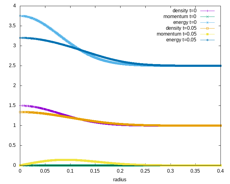
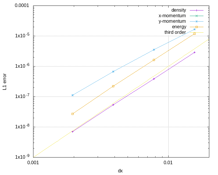
Figure 3: Convergence study. Left: Setup at initial time and at $t=0.05$, shown as scatter plot as a function of radius, computed on a $256\times 256$ grid. Right: $L^{1}$ error of the numerical solution of the point values.

4.2 Spherical shock tube

As a first test with discontinuities, Figure 4 shows a 2-dimensional version of Sod’s shock tube:

$$\rho_{0}(x,y) =\begin{cases}1&r<0.3\\ 0.125&\text{else}\end{cases} p_{0}(x,y) =\begin{cases}1&r<0.3\\ 0.1&\text{else}\end{cases}$$ (51)

$$u_{0}(x,y) =v_{0}(x,y)=0$$ (52)

with $r=\sqrt{(x-\frac{1}{2})^{2}+(y-\frac{1}{2})^{2}}$. One observes that the limiting is successful in suppressing oscillations. Global continuity does not impede Active Flux from converging to weak solutions, because the update of the averages is conservative and fulfills a version of the Lax-Wendroff-theorem ([Abg22]).

Figure 4: Radial scatter plot of the two-dimensional version of Sod’s shock tube solved on a $100\times 100$ grid. The solid line shows a finely resolved solution of the one-dimensional, radial Euler equations obtained with a standard Finite Volume method. Left: No limiting. Right: Limiting used.

4.3 Multi-dimensional Riemann problems

In [LL98], particular multi-dimensional Riemann problems were studied, designed such that the one-dimensional Riemann problems outside the central interaction region result in elementary waves. Inside the interaction region these Riemann problems display a lot of sophisticated structure. They shall illustrate the ability of the proposed method to solve complex interactions of shocks, rarefactions and slip lines. All the Riemann problems shown in Figure 5 are solved on grids with $\Delta x=\Delta y=\frac{1}{200}$ (double of what has been used in the original publication) with a domain slightly larger than the one shown (to exclude the influence of boundary conditions). A CFL number of 0.05 was used, as well as limiting, as described in Section 3. Figures 6–7 show a comparison between results obtained with and without limiting. It seems that the intricate structures in the interaction region are not significantly smeared out by the limiting while oscillations at shocks are very efficiently suppressed.

Figure 5: Multi-dimensional Riemann problems solved on a grid with $\Delta x=\Delta y=\frac{1}{200}$ using limiting as described in Section 3. Configurations 6 (top left), 11 (top right), 12 (bottom left) and 16 (bottom right) from [LL98] are shown. Color-coded is density.

Figure 6: Influence of limiting on the central region in Configuration 12. Left: Limiting off. Right: Limiting on. Without limiting one observes some undershoots inside the vortices. The structure of the solution feature is, however, not degraded by applying the limiter.

Figure 7: Influence of limiting on Configuration 12. Density is shown along the lines $x=0.4325$ and $x=0.7525$ (as indicated in the inset). One observes that limiting successfully removes spurious oscillations in the vicinity of discontinuities. However, it also gently shifts the location of the central double-vortex and smears out the feature along the $x=y$ diagonal in the first quadrant.

4.4 Kelvin-Helmholtz instability

A special kind of a Kelvin-Helmholtz instability triggered by the passage of an acoustic wave has been used in [MRKG03] to assess the properties of the numerical method for subsonic flow. The initial data are

$$\rho_{0}(x,y) =1+\frac{\mathcal{M}}{5}\psi(x)+\varphi(y) u_{0}(x,y) =\sqrt{\gamma}\psi(x)$$ (53)

$$p_{0}(x,y) =\frac{1}{\mathcal{M}^{2}}+\frac{1}{\mathcal{M}}\gamma\psi(x) v_{0}(x,y) =0$$ (54)

with

$$\varphi(y) :=\begin{cases}2\mathcal{M}y&y<4\\ 2\mathcal{M}(y-4)-0.4&\text{else}\end{cases} \psi(x) :=1+\cos(\pi\mathcal{M}x)$$ (55)

The restriction of these initial data to the $x$-direction only

$$\rho_{0}^{x}(x) :=1+\frac{\mathcal{M}}{5}\psi(x) u_{0}^{x}(x) :=\sqrt{\gamma}\psi(x)$$ (56)

$$p_{0}^{x}(x) :=\frac{1}{\mathcal{M}^{2}}+\frac{1}{\mathcal{M}}\gamma\psi(x)$$ (57)

is a right-running sound wave: The linearized Euler equations

$$\partial_{t}\rho^{x}(t,x)+\bar{\rho}\partial_{x}u^{x}(t,x) =0$$ (58)

$$\partial_{t}u^{x}(t,x)+\frac{1}{\bar{\rho}}\partial_{x}p^{x}(t,x) =0$$ (59)

$$\partial_{t}p^{x}(t,x)+\bar{\rho}c^{2}\partial_{x}u^{x}(t,x) =0$$ (60)

are solved by

$$\rho^{x}(t,x) =\rho_{0}^{x}(x-ct) u^{x}(t,x) =u_{0}^{x}(x-ct) p^{x}(t,x) =p_{0}^{x}(x-ct)$$ (61)

with $c^{2}=\frac{5\gamma}{\mathcal{M}^{2}}$ and $\bar{\rho}=\frac{1}{\sqrt{5}}$.

The non-linearity of the full Euler equations leads to a self-steepening of the sound wave. Additionally, due to the density change in $y$-direction, a shear flow is induced, which causes a Kelvin-Helmholtz instability. Here we show this setup on grids of $400\times 80$ (Figure 8) and $800\times 160$ (Figure 9) with a CFL of 0.15 and $\mathcal{M}=\frac{1}{20}$. No limiting was used. One observes that the method is able to adequately resolve both the instability and the sound waves passing through the domain.

Figure 8: A Kelvin-Helmholtz instability is triggered by the passage of an acoustic wave. The setup is computed on a $400\times 80$ grid without using limiting. Density is shown at times $t=3,6,9,12$.

Figure 9: Same setup as Figure 8, but on a grid of $800\times 160$.

5 Conclusions

Active Flux combines aspects of Finite Volume and Finite Element methods. The evolution of cell averages ensures shock-capturing properties, while the incorporation of point values at cell interfaces leads to a globally continuous reconstruction. The incorporation of additional degrees of freedom and thus the compact nature of the stencil makes the method high-order, but efficient for parallelization or the implementation of boundary conditions. The shared degrees of freedom imply less memory cost than DG methods. Finally, point values do not need to be expressed in conservative variables, i.e. Active Flux offers more freedom than conventional approaches.

The continuous reconstruction is of course the great difference to Godunov methods. There are, however, certain parallels between the history of development of Godunov methods and of Active Flux: Both started out as fully discrete methods requiring a fairly complex and expensive ingredient: an exact Riemann solver in the case of Godunov methods and an exact evolution operator in the case of Active Flux. Both can be understood as exact solutions for different IVPs: Riemann problem data in the case of Godunov methods and continuous, piecewise parabolic data in case of Active Flux. Then, for both types of methods there was a quest for simpler and more flexible approaches, with the passage from fully discrete methods to semi-discrete methods. For Godunov methods, for example, approximate Riemann solvers came up, and for Active Flux, approximate evolution operators were studied (e.g. in [Bar21]). However, due to the inherent high-order nature of Active Flux these latter needed to have high order of accuracy, and hence were non-trivial to find. Once Active Flux was rephrased as a semi-discrete method ([Abg22, AB23a]), these difficulties were overcome, for it is easy to derive spatial discretizations that use the degrees of freedom of Active Flux and to immediately write down evolution equations for the point values. The semi-discrete problem can then be integrated in time using standard methods.

To show that such an Active Flux method can be successfully used to solve the multi-dimensional Euler equations is the aim of the present work. One finds that, endowed with a limiting strategy, Active Flux is indeed able to easily solve complex flow problems. This has been demonstrated here for examples of multi-dimensional Riemann problems and for subsonic flows. The approach is generic and can immediately be applied to other hyperbolic systems of conservation laws. Further research is necessary to understand the theoretical aspects of this method, such as entropy inequalities. Future work will also be directed towards improving and simplifying the limiting and towards preservation of physical conditions such as positivity of the pressure.

Appendix A Detailed derivation of the multi-dimensional limiting

A.1 Piecewise-biparabolic reconstruction

If none of the edges needs to be limited, then the natural choice of the reconstruction is biparabolic, as it has been used already since [BHKR19, HKS19]. In presence of limited edges the reconstruction shall be defined in a piecewise fashion, subdividing the cell into quadrants or halves. If the discrete data fulfill condition (31), it is then tested (in an approximate way) whether this reconstruction fulfills $m\leq q_{\text{recon}}(x)\leq M$. In case not, it is discarded and replaced by the plateau reconstruction of Section A.2.

However, if one of the edges is reconstructed as a hat, then something else needs to be done inside the cell in order to ensure continuity. We generally choose to subdivide the cell into regions (quadrants or halves, depending on the situation) and to reconstruct biparabolically in every such region while maintaining global continuity.

Linearity of the problem (in the point values and the average) shall be exploited by considering the average and all point values apart from $q_{\text{SW}},q_{\text{W}},q_{\text{NW}}$ to vanish:

Definition A.1.

Consider all point values apart from $q_{\text{SW}},q\text{W},q_{\text{NW}},q_{\text{C}}$ and the average $\bar{q}$ to vanish. Then a reconstruction of the cell that interpolates these values pointwise and whose average agrees with $\bar{q}$ is called the edge-basis-function $q_{\text{recon}}^{\text{W}}$ of the W-edge:

$$q_{\text{recon}}^{\text{W}}\left(-\frac{\Delta x}{2},\frac{\Delta y}{2}\right) =q_{\text{NW}} q_{\text{recon}}^{\text{W}}\left(-\frac{\Delta x}{2},0\right) =q_{\text{W}}$$ (62)

$$q_{\text{recon}}^{\text{W}}\left(-\frac{\Delta x}{2},-\frac{\Delta y}{2}\right) =q_{\text{SW}} \frac{1}{\Delta x\Delta y}\int_{-\frac{\Delta x}{2}}^{\frac{\Delta x}{2}}\int_{-\frac{\Delta y}{2}}^{\frac{\Delta y}{2}}q_{\text{recon}}^{\text{W}}(x,y)\mathrm{d}x\mathrm{d}y =\bar{q}$$ (63)

Similar notions shall be used for the other edges.

Observe that an edge-basis-function is a reconstruction of the entire cell. In the following, only the edge-basis-functions for the W-edge shall be given explicitly, as those for the other edges can be obtained by rotation, as long as $\Delta y=\Delta x$ (otherwise some rescaling is necessary).

Theorem A.1.

If the edge-basis-function for the W-edge is

$$q_{\text{recon}}^{\text{W}}(q_{\text{SW}},q_{\text{W}},q_{\text{NW}},x,y,\text{S},\text{N},\text{W},\bar{q})$$ (64)

then the other basis functions are

$$q_{\text{recon}}^{\text{S}}(q_{\text{SE}},q_{\text{S}},q_{\text{SW}},x,y,\text{E},\text{W},\text{S},\bar{q}) =q_{\text{recon}}^{\text{W}}(q_{\text{SE}},q_{\text{S}},q_{\text{SW}},y,-x,\text{E},\text{W},\text{S},\bar{q})$$ (65)

$$q_{\text{recon}}^{\text{N}}(q_{\text{NW}},q_{\text{N}},q_{\text{NE}},x,y,\text{W},\text{E},\text{N},\bar{q}) =q_{\text{recon}}^{\text{W}}(q_{\text{NW}},q_{\text{N}},q_{\text{NE}},-y,x,\text{W},\text{E},\text{N},\bar{q})$$ (66)

$$q_{\text{recon}}^{\text{E}}(q_{\text{NE}},q_{\text{E}},q_{\text{SE}},x,y,\text{N},\text{S},\text{E},\bar{q}) =q_{\text{recon}}^{\text{W}}(q_{\text{NE}},q_{\text{E}},q_{\text{SE}},-x,-y,\text{N},\text{S},\text{E},\bar{q})$$ (67)

The edge-basis-function depends on $q_{\text{SW}},q\text{W},q_{\text{NW}}$, on whether the reconstruction of the W-edge is parabolic or hat, and – this complicates things a little – on whether the neighbouring edges (S and N) are reconstructed as hats or as parabolae. This is necessary due to global continuity and because the corner values $q_{\text{SW}},q\text{NW}$ are shared with the S- and N-edges. As mentioned before, the value $q_{\text{C}}$ of the reconstruction at the cell center is chosen such that the average of the reconstruction agrees with the given one (zero for edge-basis-functions).

The final reconstruction is obtained through summation:

Theorem A.2.

The following reconstruction $q_{\text{recon}}$ interpolates all the point values along the boundary of the cell and its average agrees with the given cell average:

$$q_{\text{recon}}(x,y) :=q_{\text{recon}}^{\text{W}}\left(\frac{q_{\text{SW}}}{2},q_{\text{W}},\frac{q_{\text{NW}}}{2},x,y,\text{S},\text{N},\text{W},\frac{\Delta\bar{q}}{4}\right)$$ (68)

$$+q_{\text{recon}}^{\text{S}}\left(\frac{q_{\text{SE}}}{2},q_{\text{S}},\frac{q_{\text{SW}}}{2},x,y,\text{E},\text{W},\text{S},\frac{\Delta\bar{q}}{4}\right)$$

$$+q_{\text{recon}}^{\text{N}}\left(\frac{q_{\text{NW}}}{2},q_{\text{N}},\frac{q_{\text{NE}}}{2},x,y,\text{W},\text{E},\text{N},\frac{\Delta\bar{q}}{4}\right)$$

$$+q_{\text{recon}}^{\text{E}}\left(\frac{q_{\text{NE}}}{2},q_{\text{E}},\frac{q_{\text{SE}}}{2},x,y,\text{N},\text{S},\text{E},\frac{\Delta\bar{q}}{4}\right)$$

$$+(\bar{q}-\Delta\bar{q})$$

where $\Delta\bar{q}:=\bar{q}-\frac{q_{\text{SW}}+q_{\text{W}}+q_{\text{NW}}+q_{\text{N}}+q_{\text{NE}}+q_{\text{E}}+q_{\text{SE}}+q_{\text{S}}}{8}$. Moreover, as all the point values tend to $\bar{q}$,

$$q_{\text{recon}}(x,y)\to\bar{q}$$ (69)

for all $x,y$.

Proof.

The pointwise interpolation property is clear because, for example,

$$q_{\text{recon}}\left(\frac{\Delta x}{2},\frac{\Delta y}{2}\right) =q_{\text{recon}}^{\text{N}}\left(\frac{q_{\text{NW}}}{2},q_{\text{N}},\frac{q_{\text{NE}}}{2},\frac{\Delta x}{2},\frac{\Delta y}{2},\text{W},\text{E},\text{N},\frac{\Delta\bar{q}}{4}\right)$$ (70)

$$+ q_{\text{recon}}^{\text{E}}\left(\frac{q_{\text{NE}}}{2},q_{\text{E}},\frac{q_{\text{SE}}}{2},\frac{\Delta x}{2},\frac{\Delta y}{2},\text{N},\text{S},\text{E},\frac{\Delta\bar{q}}{4}\right)$$ (71)

$$=\frac{q_{\text{NE}}}{2}+\frac{q_{\text{NE}}}{2}=q_{\text{NE}}$$ (72)

The correctness of the average follows from

$$\frac{1}{\Delta x\Delta y}\int_{-\frac{\Delta x}{2}}^{\frac{\Delta x}{2}}\int_{-\frac{\Delta y}{2}}^{\frac{\Delta y}{2}}q_{\text{recon}}^{\text{W}}(x,y)\mathrm{d}x\mathrm{d}y=4\cdot\frac{\Delta\bar{q}}{4}+\bar{q}-\Delta\bar{q}=\bar{q}$$ (73)

Finally, property (69) is trivial if $\bar{q}=0$, because the reconstruction is linear in all the point values and in the average, and thus $q_{\text{recon}}(x,y)\to 0$ uniformly in this case. If the point values tend to $\bar{q}\neq 0$, then $\Delta\bar{q}\to 0$ and thus

$$q_{\text{recon}}(x,y)\to 0+\bar{q}-\Delta\bar{q}\to\bar{q}$$ (74)

∎

Remark A.1.

: One might think that it would be sufficient to define the reconstruction as

$$q_{\text{recon}}^{\text{W}}\left(\frac{q_{\text{SW}}}{2},q_{\text{W}},\frac{q_{\text{NW}}}{2},x,y,\text{S},\text{N},\text{W},\frac{\bar{q}}{4}\right)+q_{\text{recon}}^{\text{S}}\left(\frac{q_{\text{SE}}}{2},q_{\text{S}},\frac{q_{\text{SW}}}{2},x,y,\text{E},\text{W},\text{S},\frac{\bar{q}}{4}\right)$$ (75)

$$+ q_{\text{recon}}^{\text{N}}\left(\frac{q_{\text{NW}}}{2},q_{\text{N}},\frac{q_{\text{NE}}}{2},x,y,\text{W},\text{E},\text{N},\frac{\bar{q}}{4}\right)+q_{\text{recon}}^{\text{E}}\left(\frac{q_{\text{NE}}}{2},q_{\text{E}},\frac{q_{\text{SE}}}{2},x,y,\text{N},\text{S},\text{E},\frac{\bar{q}}{4}\right)$$ (76)

This function also has the interpolation properties in Theorem A.2. However, in the limit of all the point values converging to $\bar{q}$, property (69) is not guaranteed. Linearity merely implies that in the limit, $q_{\text{recon}}$ will be proportional to $\bar{q}$, but it can still have a non-trivial dependence on $x,y$.

If the reconstruction happens on the unit square, then $\Delta x=\Delta y=1$ should be used in the formulas below. The sketches of the interpolation problem are encoded as follows: denotes the central value $q_{\text{C}}$, / denotes a value that is not on the W edge and thus zero (gray if it is not used in the interpolation), / denotes one of the values $q_{\text{NW}}$, $q_{\text{W}}$, $q_{\text{SW}}$ (gray if it is not used in the interpolation). Values marked with an arrow do not, in principle, need to be included in the interpolation stencil, but are included here. The colored area denotes the support of the different functions that make up the piecewise defined reconstruction. denotes an edge that is reconstructed linearly, in other words, as part of the interpolation procedure, we impose that the restriction of the reconstruction onto that edge is linear (the quadratic term vanishing).

In many cases, the reconstruction is (piecewise) biparabolic, i.e. of the form

$$(a_{0}+a_{1}x+a_{2}x^{2})+(a_{3}+a_{4}x+a_{5}x^{2})y+(a_{6}+a_{7}x+a_{8}x^{2})y^{2}$$ (77)

In the following, biparabolic reconstructions are given by specifying the values of these 9 coefficients.

A.1.1 Parabolic reconstruction on W edge

If edges W, S and N are all reconstructed parabolically, then the W-edge-basis-function is a biparabolic function. If either S or N (or both) are reconstructed as hat functions, the reconstruction in the cell is defined piecewise: the left and the rights halves of the cell have individual biparabolic reconstructions, which are joined in a continuous fashion.

Parabolic reconstruction on both neighbouring edges

If both neighbouring edges (N and S) are reconstructed parabolically, then the reconstruction inside the cell is the trivial biparabolic reconstruction (see Figure 10):

$$q_{\text{recon}}^{\text{W}} =\left\{a_{0}=q_{\text{C}},a_{1}=-\frac{q_{\text{W}}}{\Delta x},a_{2}=-\frac{2(2q_{\text{C}}-q_{\text{W}})}{\Delta x^{2}},a_{3}=0,a_{4}=-\frac{q_{\text{NW}}-q_{\text{SW}}}{\Delta x\Delta y},\right.$$ (78)

$$\phantom{mmm}\left.a_{5}=\frac{2(q_{\text{NW}}-q_{\text{SW}})}{\Delta x^{2}\Delta y},a_{6}=-\frac{4q_{\text{C}}}{\Delta y^{2}},a_{7}=-\frac{2(q_{\text{NW}}+q_{\text{SW}}-2q_{\text{W}})}{\Delta x\Delta y^{2}},\right.$$

$$\phantom{mmm}\left.a_{8}=\frac{4(4q_{\text{C}}+q_{\text{NW}}+q_{\text{SW}}-2q_{\text{W}})}{\Delta x^{2}\Delta y^{2}}\right\}$$

$$q_{\text{C}} =\frac{1}{16}(36\bar{q}-q_{\text{NW}}-q_{\text{SW}}-4q_{\text{W}})$$ (79)

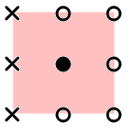
Figure 10: All edges are reconstructed parabolically, and the corresponding edge-basis-function is a simple biparabolic interpolation. $q_{\text{NW}}=1.6$, $q_{\text{W}}=1.35$, $q_{\text{SW}}=0.6$.

Hat reconstruction on both neighbouring edges

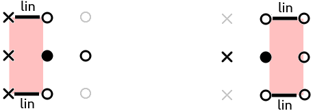
Figure 11: Top: The case of both neighbouring edges reconstructed using hat functions, while the primary edge is reconstructed parabolically. Bottom: The W edge is reconstructed parabolically, while the two neighbouring reconstructions are hat functions. $q_{\text{NW}}=1.6$, $q_{\text{W}}=1.35$, $q_{\text{SW}}=0.6$.

The interpolation problem is shown in Figure 11.

$$q_{\text{recon}}^{\text{W}}\Big{|}_{x<0} =\left\{a_{0}=q_{\text{C}},a_{1}=-\frac{q_{\text{W}}}{\Delta x},a_{2}=-\frac{2(2q_{\text{C}}-q_{\text{W}})}{\Delta x^{2}},a_{3}=0,a_{4}=-\frac{2(q_{\text{NW}}-q_{\text{SW}})}{\Delta x\Delta y},\right.$$ (80)

$$\phantom{mmm}\left.a_{5}=0,a_{6}=-\frac{4q_{\text{C}}}{\Delta y^{2}},a_{7}=-\frac{4(q_{\text{NW}}+q_{\text{SW}}-q_{\text{W}})}{\Delta x\Delta y^{2}},a_{8}=\frac{8(2q_{\text{C}}-q_{\text{W}})}{\Delta x^{2}\Delta y^{2}}\right\}$$

$$q_{\text{recon}}^{\text{W}}\Big{|}_{x\geq 0} =\left\{a_{0}=q_{\text{C}},a_{1}=-\frac{q_{\text{W}}}{\Delta x},a_{2}=-\frac{2(2q_{\text{C}}-q_{\text{W}})}{\Delta x^{2}},a_{3}=0,a_{4}=0,\right.$$ (81)

$$\phantom{mmm}\left.a_{5}=0,a_{6}=-\frac{4q_{\text{C}}}{\Delta y^{2}},a_{7}=\frac{4q_{\text{W}}}{\Delta x\Delta y^{2}},a_{8}=\frac{8(2q_{\text{C}}-q_{\text{W}})}{\Delta x^{2}\Delta y^{2}}\right\}$$

$$q_{\text{C}} =\frac{1}{32}(72\bar{q}-3(q_{\text{NW}}+q_{\text{SW}})-8q_{\text{W}})$$ (82)

Hat reconstruction on just one neighbouring edge

If the N edge is reconstructed using a hat function, and both the W-edge and the S-edge parabolically, then one reconstructs the cell as follows (Figure 12):

$$q_{\text{recon}}^{\text{W}}\Big{|}_{x<0} =\left\{a_{0}=q_{\text{C}},a_{1}=-\frac{q_{\text{W}}}{\Delta x},a_{2}=-\frac{2(2q_{\text{C}}-q_{\text{W}})}{\Delta x^{2}},a_{3}=0,a_{4}=-\frac{2q_{\text{NW}}-q_{\text{SW}}}{\Delta x\Delta y},\right.$$ (83)

$$\phantom{mmm}\left.a_{5}=-\frac{2q_{\text{SW}}}{\Delta x^{2}\Delta y},a_{6}=-\frac{4q_{\text{C}}}{\Delta y^{2}},a_{7}=-\frac{2(2q_{\text{NW}}+q_{\text{SW}}-2q_{\text{W}})}{\Delta x\Delta y^{2}},\right.$$

$$\phantom{mmm}\left.a_{8}=\frac{4(4q_{\text{C}}+q_{\text{SW}}-2q_{\text{W}})}{\Delta x^{2}\Delta y^{2}}\right\}$$

$$q_{\text{recon}}^{\text{W}}\Big{|}_{x\geq 0} =\left\{a_{0}=q_{\text{C}},a_{1}=-\frac{q_{\text{W}}}{\Delta x},a_{2}=-\frac{2(2q_{\text{C}}-q_{\text{W}})}{\Delta x^{2}},a_{3}=0,a_{4}=\frac{q_{\text{SW}}}{\Delta x\Delta y},\right.$$ (84)

$$\phantom{mmm}\left.a_{5}=-\frac{2q_{\text{SW}}}{\Delta x^{2}\Delta y},a_{6}=-\frac{4q_{\text{C}}}{\Delta y^{2}},a_{7}=-\frac{2(q_{\text{SW}}-2q_{\text{W}})}{\Delta x\Delta y^{2}},\right.$$

$$\phantom{mmm}\left.a_{8}=\frac{4(4q_{\text{C}}+q_{\text{SW}}-2q_{\text{W}})}{\Delta x^{2}\Delta y^{2}}\right\}$$

$$q_{\text{C}} =\frac{1}{32}(72\bar{q}-3q_{\text{NW}}-2(q_{\text{SW}}+4q_{\text{W}}))$$ (85)

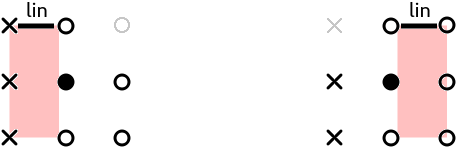
Figure 12: Top: The case of the N edge reconstructed using hat functions, while the primary edge and the S-edge is reconstructed parabolically. Bottom: The W and S edge is reconstructed parabolically, while the N edge is reconstructed using a hat function. $q_{\text{NW}}=1.6$, $q_{\text{W}}=1.35$, $q_{\text{SW}}=0.6$.

If it is the S edge, then (Figure 13):

$$q_{\text{recon}}^{\text{W}}\Big{|}_{x<0} =\left\{a_{0}=q_{\text{C}},a_{1}=-\frac{q_{\text{W}}}{\Delta x},a_{2}=-\frac{2(2q_{\text{C}}-q_{\text{W}})}{\Delta x^{2}},a_{3}=0,a_{4}=-\frac{q_{\text{NW}}-2q_{\text{SW}}}{\Delta x\Delta y},\right.$$ (86)

$$\phantom{mmm}\left.a_{5}=\frac{2q_{\text{NW}}}{\Delta x^{2}\Delta y},a_{6}=-\frac{4q_{\text{C}}}{\Delta y^{2}},a_{7}=-\frac{2(q_{\text{NW}}+2q_{\text{SW}}-2q_{\text{W}})}{\Delta x\Delta y^{2}},\right.$$

$$\phantom{mmm}\left.a_{8}=\frac{4(4q_{\text{C}}+q_{\text{NW}}-2q_{\text{W}})}{\Delta x^{2}\Delta y^{2}}\right\}$$

$$q_{\text{recon}}^{\text{W}}\Big{|}_{x\geq 0} =\left\{a_{0}=q_{\text{C}},a_{1}=-\frac{q_{\text{W}}}{\Delta x},a_{2}=-\frac{2(2q_{\text{C}}-q_{\text{W}})}{\Delta x^{2}},a_{3}=0,a_{4}=-\frac{q_{\text{NW}}}{\Delta x\Delta y},\right.$$ (87)

$$\phantom{mmm}\left.a_{5}=\frac{2q_{\text{NW}}}{\Delta x^{2}\Delta y},a_{6}=-\frac{4q_{\text{C}}}{\Delta y^{2}},a_{7}=-\frac{2(q_{\text{NW}}-2q_{\text{W}})}{\Delta x\Delta y^{2}},\right.$$

$$\phantom{mmm}\left.a_{8}=\frac{4(4q_{\text{C}}+q_{\text{NW}}-2q_{\text{W}})}{\Delta x^{2}\Delta y^{2}}\right\}$$

$$q_{\text{C}} =\frac{1}{32}(72\bar{q}-2q_{\text{NW}}-3q_{\text{SW}}-8q_{\text{W}})$$ (88)

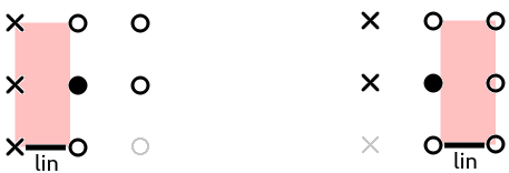
Figure 13: Top: The case of the S edge reconstructed using hat functions, while the primary edge is reconstructed parabolically. Bottom: The W and N edge is reconstructed parabolically, while the S edge is reconstructed using a hat function. $q_{\text{NW}}=1.6$, $q_{\text{W}}=1.35$, $q_{\text{SW}}=0.6$.

Proof of continuity

It is obvious from the sketches of the interpolation problem in Figures 10–13 that the reconstructions interpolate the values on the cell interfaces. What remains to be shown is that the piecewise defined reconstruction is continuous:

Theorem A.3.

The reconstructions from Sections A.1.1–A.1.1 are continuous along the line $x=0$ where the two pieces are joined.

Proof.

As is obvious from the sketches of the interpolation problems in Figures 11–13, the three points along $x=0$, i.e.

$$q_{\text{recon}}\left(0,\frac{\Delta y}{2}\right) =0 q_{\text{recon}}\left(0,0\right) =q_{\text{C}} q_{\text{recon}}\left(0,-\frac{\Delta y}{2}\right) =0$$ (89)

are part of the interpolation. Recall that the restriction of a biparabolic function onto the straight line $x=0$ is a parabola in $y$, and that the latter is uniquely defined by three points. Therefore, all the values of the reconstruction along $x=0$ agree for all the reconstructions presented in Sections A.1.1–A.1.1. ∎

A.1.2 Hat reconstruction on W edge

If the W-edge is reconstructed as a hat function, then necessarily one needs to consider a piecewise defined reconstruction with the pieces joined along $y=0$. The reconstruction in each piece only depends on whether the other adjacent edge is reconstructed parabolically or as a hat function. One thus has less cases to consider.

Consider the top piece, i.e. the one defined on $[-\frac{\Delta x}{2},\frac{\Delta x}{2}]\times[0,\frac{\Delta y}{2}]$. It is bordered by the N-edge. If the N-edge is reconstructed as a hat function then one needs additionally to define the reconstruction piecewise in the left and right halves (joined along $x=0$), i.e. the reconstruction is piecewise by quadrant. This is not necessary if the N-edge is reconstructed parabolically.

Parabolic reconstruction on at least one neighbouring edge

Here, the situation is considered in which either the N-edge or the S-edge are reconstructed as parabolae. Then it is possible to provide a biparabolic reconstruction of, respectively, the top or bottom half of the cell.

These cases can occur individually or simultaneously. If both the N-edge and the S-edge are reconstructed parabolically, then the entire reconstruction of the cell is given by the two pieces given in (90)–(92). If, for example, the N-edge is reconstructed parabolically, and the S-edge as a hat function, then the top piece of the reconstruction in the cell is to be taken from (90), while the bottom piece used should be the one from (97)–(98) in Section A.1.2.

See Figure 14 for the setup of the interpolation problem.

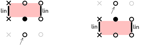
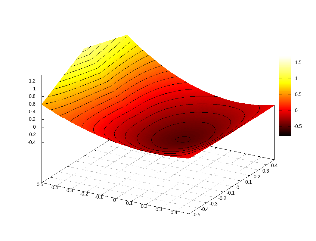
Figure 14: Top: The case of the neighbouring edges reconstructed using parabolas, while the primary edge is reconstructed using the hat function. Bottom: The W edge is reconstructed as a hat function, the other edges are reconstructed parabolically. $q_{\text{NW}}=1$, $q_{\text{W}}=1.5$, $q_{\text{SW}}=0$.

$$q_{\text{recon}}^{W}\Big{|}_{y\geq 0} =\left\{a_{0}=q_{\text{C}},a_{1}=-\frac{q_{\text{W}}}{\Delta x},a_{2}=-\frac{2(2q_{\text{C}}-q_{\text{W}})}{\Delta x^{2}},a_{3}=0,a_{4}=-\frac{2(q_{\text{NW}}-q_{\text{W}})}{\Delta x\Delta y},\right.$$ (90)

$$\phantom{mmm}\left.a_{5}=\frac{4(q_{\text{NW}}-q_{\text{W}})}{\Delta x^{2}\Delta y},a_{6}=-\frac{4q_{\text{C}}}{\Delta y^{2}},a_{7}=0,a_{8}=\frac{16q_{\text{C}}}{\Delta x^{2}\Delta y^{2}}\right\}$$

$$\frac{1}{\Delta x\Delta y} \int_{y\geq 0}q_{\text{recon}}\,\mathrm{d}x\mathrm{d}y=\frac{2q_{\text{C}}}{9}+\frac{q_{\text{NW}}+q_{\text{W}}}{24}$$ (91)

$$q_{\text{recon}}^{W}\Big{|}_{y<0} =\left\{a_{0}=q_{\text{C}},a_{1}=-\frac{q_{\text{W}}}{\Delta x},a_{2}=-\frac{2(2q_{\text{C}}-q_{\text{W}})}{\Delta x^{2}},a_{3}=0,a_{4}=\frac{2(q_{\text{SW}}-q_{\text{W}})}{\Delta x\Delta y},\right.$$ (92)

$$\phantom{mmm}\left.a_{5}=-\frac{4(q_{\text{SW}}-q_{\text{W}})}{\Delta x^{2}\Delta y},a_{6}=-\frac{4q_{\text{C}}}{\Delta y^{2}},a_{7}=0,a_{8}=\frac{16q_{\text{C}}}{\Delta x^{2}\Delta y^{2}}\right\}$$

$$\frac{1}{\Delta x\Delta y} \int_{y<0}q_{\text{recon}}\,\mathrm{d}x\mathrm{d}y=\frac{2q_{\text{C}}}{9}+\frac{q_{\text{SW}}+q_{\text{W}}}{24}$$ (93)

Hat reconstruction on at least one neighbouring edge

In this case the reconstruction is additionally defined piecewise on each quadrant. The biparabolic reconstructions are obtained from interpolation problems shown in Figure 15.

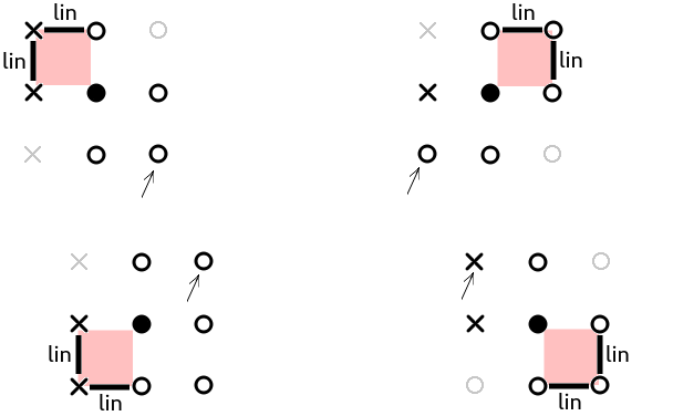
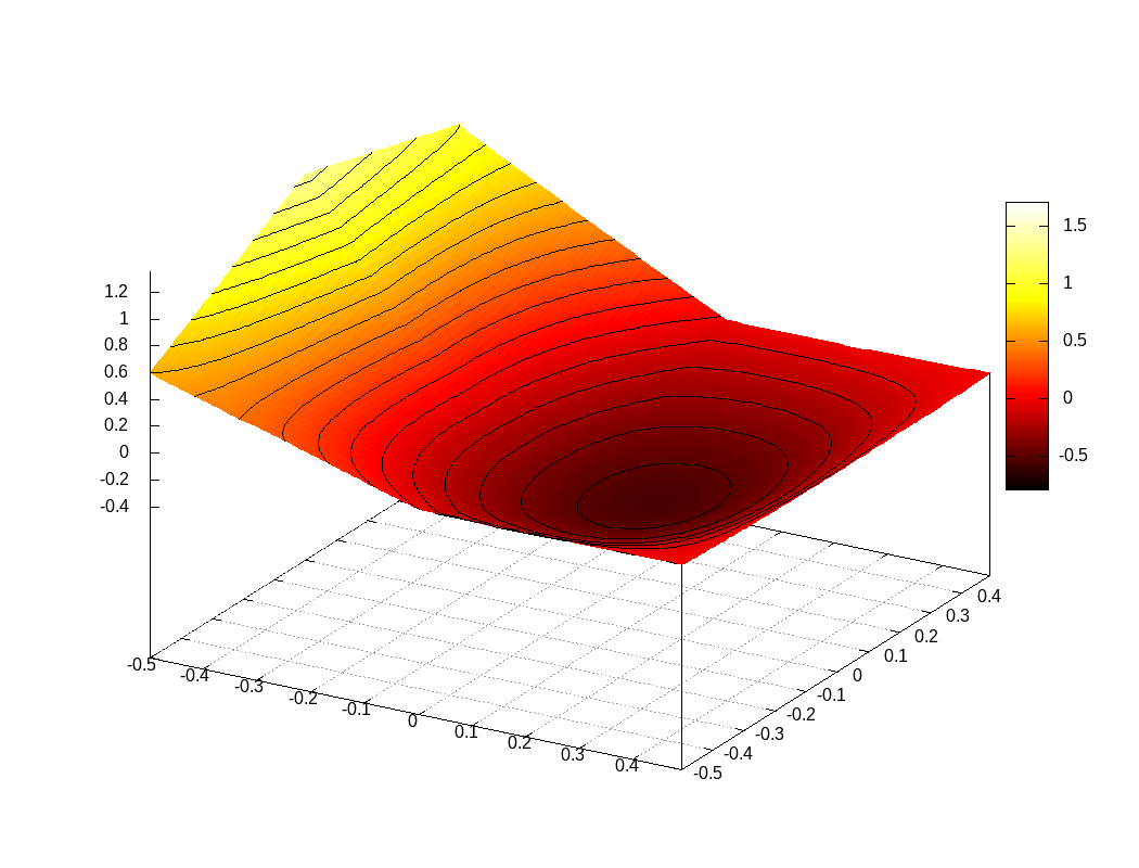
Figure 15: Top: The case of (possibly) all three edges reconstructed using hat functions. The reconstruction inside the cell is defined on four quadrants. Middle: The W edge is reconstructed as a hat function, and also N (left) / S (right). Bottom: All edges are reconstructed as hat functions.

If the N edge is reconstructed as a hat function, then the top half $[-\frac{\Delta x}{2},\frac{\Delta x}{2}]\times[0,\frac{\Delta y}{2}]$ of the cell is to be reconstructed as

$$q_{\text{recon}}^{\text{W}}\Big{|}_{y\geq 0,x<0} =\left\{a_{0}=q_{\text{C}},a_{1}=-\frac{q_{\text{W}}}{\Delta x},a_{2}=-\frac{2(2q_{\text{C}}-q_{\text{W}})}{\Delta x^{2}},a_{3}=0,a_{4}=-\frac{3q_{\text{NW}}-2q_{\text{W}}}{\Delta x\Delta y},\right.$$ (94)

$$\phantom{mmm}\left.a_{5}=\frac{2(q_{\text{NW}}-2q_{\text{W}})}{\Delta x^{2}\Delta y},a_{6}=-\frac{4q_{\text{C}}}{\Delta y^{2}},a_{7}=-\frac{2q_{\text{NW}}}{\Delta x\Delta y^{2}},\right.$$

$$\phantom{mmm}\left.a_{8}=\frac{4(4q_{\text{C}}-q_{\text{NW}})}{\Delta x^{2}\Delta y^{2}}\right\}$$

$$q_{\text{recon}}^{\text{W}}\Big{|}_{y\geq 0,x\geq 0} =\left\{a_{0}=q_{\text{C}},a_{1}=-\frac{q_{\text{W}}}{\Delta x},a_{2}=-\frac{2(2q_{\text{C}}-q_{\text{W}})}{\Delta x^{2}},a_{3}=0,a_{4}=\frac{q_{\text{SW}}}{\Delta x\Delta y},\right.$$ (95)

$$\phantom{mmm}\left.a_{5}=-\frac{2q_{\text{SW}}}{\Delta x^{2}\Delta y},a_{6}=-\frac{4q_{\text{C}}}{\Delta y^{2}},a_{7}=-\frac{2(q_{\text{SW}}-2q_{\text{W}})}{\Delta x\Delta y^{2}},\right.$$

$$\phantom{mmm}\left.a_{8}=\frac{4(4q_{\text{C}}+q_{\text{SW}}-2q_{\text{W}})}{\Delta x^{2}\Delta y^{2}}\right\}$$

$$\frac{1}{\Delta x\Delta y} \int_{y\geq 0}q_{\text{recon}}\,\mathrm{d}x\mathrm{d}y=\frac{2q_{\text{C}}}{9}+\frac{1}{576}(35q_{\text{NW}}+q_{\text{SW}}+22q_{\text{W}})$$ (96)

If the S edge is reconstructed as a hat function, then the reconstruction reads

$$q_{\text{recon}}^{\text{W}}\Big{|}_{y<0,x<0} =\left\{a_{0}=q_{\text{C}},a_{1}=-\frac{q_{\text{W}}}{\Delta x},a_{2}=-\frac{2(2q_{\text{C}}-q_{\text{W}})}{\Delta x^{2}},a_{3}=0,\right.$$ (97)

$$\phantom{mmm}\left.a_{4}=-\frac{-3q_{\text{SW}}+2q_{\text{W}}}{\Delta x\Delta y},a_{5}=-\frac{2(q_{\text{SW}}-2q_{\text{W}})}{\Delta x^{2}\Delta y},a_{6}=-\frac{4q_{\text{C}}}{\Delta y^{2}},\right.$$

$$\phantom{mmm}\left.a_{7}=-\frac{2q_{\text{SW}}}{\Delta x\Delta y^{2}},a_{8}=\frac{4(4q_{\text{C}}-q_{\text{SW}})}{\Delta x^{2}\Delta y^{2}}\right\}$$

$$q_{\text{recon}}^{\text{W}}\Big{|}_{y<0,x\geq 0} =\left\{a_{0}=q_{\text{C}},a_{1}=-\frac{q_{\text{W}}}{\Delta x},a_{2}=-\frac{2(2q_{\text{C}}-q_{\text{W}})}{\Delta x^{2}},a_{3}=0,a_{4}=-\frac{q_{\text{NW}}}{\Delta x\Delta y},\right.$$ (98)

$$\phantom{mmm}\left.a_{5}=\frac{2q_{\text{NW}}}{\Delta x^{2}\Delta y},a_{6}=-\frac{4q_{\text{C}}}{\Delta y^{2}},a_{7}=-\frac{2(q_{\text{NW}}-2q_{\text{W}})}{\Delta x\Delta y^{2}},\right.$$

$$\phantom{mmm}\left.a_{8}=\frac{4(4q_{\text{C}}+q_{\text{NW}}-2q_{\text{W}})}{\Delta x^{2}\Delta y^{2}}\right\}$$

$$\frac{1}{\Delta x\Delta y} \int_{y<0}q_{\text{recon}}\,\mathrm{d}x\mathrm{d}y=\frac{2q_{\text{C}}}{9}+\frac{1}{576}(q_{\text{NW}}+35q_{\text{SW}}+22q_{\text{W}})$$ (99)

Proof of continuity

Theorem A.4.

The reconstructions in Sections A.1.2–A.1.2 are continuous along $x=0$ and along $y=0$.

Proof.

In complete analogy to the proof of Theorem A.3 one observes from the sketches of the interpolation problem in Figures 14–15 that the points along $x=0$ and $y=0$ are always included. The three points along $x=0$ and the three points along $y=0$ each define a unique parabola. ∎

A.2 Plateau-limiting

Consider a situation in which (31) is true, while the reconstruction described above exceeds $m$ or $M$. In that case, the idea of a plateau reconstruction is to introduce a rectangle a distance $\eta\Delta x$/$\eta\Delta y$ away from the cell boundary, i.e.

$$\left[\Delta x\left(-\frac{1}{2}+\eta\right),\Delta x\left(\frac{1}{2}-\eta\right)\right]\times\left[\Delta y\left(-\frac{1}{2}+\eta\right),\Delta y\left(\frac{1}{2}-\eta\right)\right]$$

with $\eta\in(0,\frac{1}{2})$ where the value of the reconstruction shall be constant and equal to $q_{\text{p}}$, a value to be determined to ensure that the average of the reconstruction equals the given average (see Figure 1 for an example). This rectangle shall be referred to as plateau. The remaining four trapezes shall be the supports of functions that continuously join the reconstruction along the edge to the plateau in the simplest possible way. Because reconstructions along edges are either parabolas or hats, every trapezoidal region is either joining the plateau to a parabola or to a hat function. $\eta$ shall be chosen in such a way that the maximum principle is guaranteed. It is clear that, as (31) is true, this can always be done by choosing $\eta$ small enough.

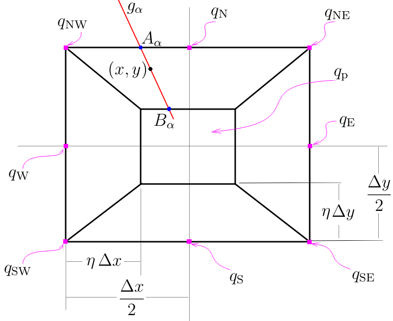
Figure 16: Sketch of the interpolation between the plateau and the boundary of the cell.

A.2.1 Interpolation in the trapezes

Consider for definiteness the northern trapeze. Define a point $A_{\alpha}:=\left(-\frac{\Delta x}{2}+\alpha\Delta x,\frac{\Delta y}{2}\right)\in\mathbb{R}^{2}$ parametrized by $\alpha\in[0,1]$. Define a point

$$B_{\alpha}:=\left(\Delta x(-\frac{1}{2}+\eta)+\alpha\Delta x(1-2\eta),\Delta y(\frac{1}{2}-\eta)\right)$$

on the northern edge of the plateau. Observe that as $\alpha$ goes from 0 to 1, both points move all the way from the left to the right on their respective edges. The straight line

$$g_{\alpha}:=\left\{(x,y):\frac{x}{\Delta x}=-\frac{1}{2}+\alpha-\left(\frac{y}{\Delta y}-\frac{1}{2}\right)(1-2\alpha)\right\}$$ (100)

connects them. Obviously, given $x$ and $y$ there is a unique

$$\alpha=\frac{\frac{x}{\Delta x}+\frac{y}{\Delta y}}{2\frac{y}{\Delta y}}=\frac{x\Delta y+y\Delta x}{2y\Delta x}$$ (101)

The idea of the reconstruction is to associate to a point $(x,y)$ the value given by a linear interpolation between the value of the reconstruction at $A_{\alpha}$ and the (constant) value $q_{\text{p}}$ at $B_{\alpha}$. In particular this means that the diagonal edges of the reconstruction (connections between the corners of the cell and the corners of the plateau) are straight lines.

The four trapezes can be reconstructed individually, because continuity along the diagonal segments where they join is already guaranteed by the above procedure. For a given trapeze, the choice of reconstruction thus merely depends on whether the adjacent edge is reconstructed parabolically (see Section A.2.2) or as a hat function (see Section A.2.3).

A.2.2 Parabolic reconstruction along the edge

The parabolic reconstruction along the N-edge is given by

$$q_{\text{parabolic}}^{\text{N}}(x)=q_{\text{N}}+\frac{x}{\Delta x}(q_{\text{NE}}-q_{\text{NW}})+2\frac{x^{2}}{\Delta x^{2}}(q_{\text{NE}}+q_{\text{NW}}-2q_{\text{N}})\qquad x\in\left[-\frac{\Delta x}{2},\frac{\Delta x}{2}\right]$$ (102)

The value of this parabolic reconstruction is sought at the location $\xi$ of point $A_{\alpha}$ with $\alpha$ given by (101):

$$\xi=\Delta x\left(-\frac{1}{2}+\frac{\frac{x}{\Delta x}\Delta y+y}{2y}\right)=\Delta x\frac{\frac{x}{\Delta x}}{2\frac{y}{\Delta y}}$$ (103)

Finally, the reconstruction at $(x,y)$ is assigned the value

$$q_{\text{recon}}^{\text{N}}(x,y) :=q_{\text{parabolic}}^{\text{N}}(\xi)+\left(y-\frac{\Delta y}{2}\right)\frac{q_{\text{p}}-q_{\text{parabolic}}^{\text{N}}(\xi)}{-\Delta y\eta}$$ (104)

$$=q_{\text{parabolic}}^{\text{N}}(\xi)\left(1+\frac{\frac{y}{\Delta y}-\frac{1}{2}}{\eta}\right)-\frac{\frac{y}{\Delta y}-\frac{1}{2}}{\eta}q_{\text{p}}$$ (105)

with

$$q_{\text{parabolic}}^{\text{N}}(\xi) =q_{\text{N}}+\frac{\hat{x}}{2\hat{y}}(q_{\text{NE}}-q_{\text{NW}})+2\left(\frac{\hat{x}}{2\hat{y}}\right)^{2}(q_{\text{NE}}+q_{\text{NW}}-2q_{\text{N}})$$ (106)

and $\hat{x}:=\frac{x}{\Delta x}$ and $\hat{y}:=\frac{y}{\Delta y}$. Observe that the reconstruction is not polynomial, but lies in

$$\mathrm{span}\left(1,\hat{x},\hat{y},\frac{\hat{x}}{\hat{y}},\frac{{\hat{x}}^{2}}{\hat{y}},\frac{{\hat{x}}^{2}}{{\hat{y}}^{2}}\right)$$ (107)

For reference we give the four reconstructions:

$$q_{\text{recon}}^{\text{trapeze W}}(x,y) =q_{\text{p}}\frac{1+2\hat{x}}{2\eta}+(-1+2\eta-2\hat{x})\left(\frac{q_{\text{W}}}{2\eta}-\frac{(q_{\text{NW}}-q_{\text{SW}})y}{4\eta\hat{x}}+\frac{(q_{\text{NW}}+q_{\text{SW}}-2q_{\text{W}})\hat{y}^{2}}{4\eta\hat{x}^{2}}\right)$$ (108)

$$q_{\text{recon}}^{\text{trapeze E}}(x,y) =q_{\text{p}}\frac{1-2\hat{x}}{2\eta}+(-1+2\eta+2\hat{x})\left(\frac{q_{\text{E}}}{2\eta}+\frac{(q_{\text{NE}}-q_{\text{SE}})\hat{y}}{4\eta\hat{x}}-\frac{(2q_{\text{E}}-q_{\text{NE}}-q_{\text{SE}})\hat{y}^{2}}{4\eta\hat{x}^{2}}\right)$$ (109)

$$q_{\text{recon}}^{\text{trapeze N}}(x,y) =q_{\text{p}}\frac{1-2\hat{y}}{2\eta}+(-1+2\eta+2\hat{y})\left(-\frac{(2q_{\text{N}}-q_{\text{NE}}-q_{\text{NW}})\hat{x}^{2}}{4\eta\hat{y}^{2}}+\frac{(q_{\text{NE}}-q_{\text{NW}})\hat{x}}{4\eta\hat{y}}+\frac{q_{\text{N}}}{2\eta}\right)$$ (110)

$$q_{\text{recon}}^{\text{trapeze S}}(x,y) =q_{\text{p}}\frac{1+2\hat{y}}{2\eta}+(1-2\eta+2\hat{y})\left(\frac{(2q_{\text{S}}-q_{\text{SE}}-q_{\text{SW}})\hat{x}^{2}}{4\eta\hat{y}^{2}}+\frac{(q_{\text{SE}}-q_{\text{SW}})\hat{x}}{4\eta\hat{y}}-\frac{q_{\text{S}}}{2\eta}\right)$$ (111)

The integrals over the four regions are

$$\frac{1}{\Delta x\Delta y}\int_{\text{trapeze W}}q_{\text{recon}}\,\mathrm{d}x\mathrm{d}y =\frac{1}{36}\eta\Big{(}6(3-4\eta)q_{\text{P}}-(2\eta-3)(4q_{\text{W}}+q_{\text{NW}}+q_{\text{SW}})\Big{)}$$ (112)

$$\frac{1}{\Delta x\Delta y}\int_{\text{trapeze E}}q_{\text{recon}}\,\mathrm{d}x\mathrm{d}y =\frac{1}{36}\eta\Big{(}6(3-4\eta)q_{\text{P}}-(2\eta-3)(4q_{\text{E}}+q_{\text{NE}}+q_{\text{SE}})\Big{)}$$ (113)

$$\frac{1}{\Delta x\Delta y}\int_{\text{trapeze N}}q_{\text{recon}}\,\mathrm{d}x\mathrm{d}y =\frac{1}{36}\eta\Big{(}6(3-4\eta)q_{\text{P}}-(2\eta-3)(4q_{\text{N}}+q_{\text{NE}}+q_{\text{NW}})\Big{)}$$ (114)

$$\frac{1}{\Delta x\Delta y}\int_{\text{trapeze S}}q_{\text{recon}}\,\mathrm{d}x\mathrm{d}y =\frac{1}{36}\eta\Big{(}6(3-4\eta)q_{\text{P}}-(2\eta-3)(4q_{\text{S}}+q_{\text{SE}}+q_{\text{SW}})\Big{)}$$ (115)

and the integral over the plateau obviously

$$\frac{1}{\Delta x\Delta y}\int_{\text{plateau}}q_{\text{recon}}\,\mathrm{d}x\mathrm{d}y=(1-2\eta)^{2}q_{\text{p}}$$ (116)

A.2.3 Hat-function reconstruction along the edge

If an edge is reconstructed using a hat-function, then the reconstruction of the trapeze follows the algorithm outlined at the beginning of Section A.2, but is naturally defined in a piecewise fashion. The reconstruction of the W-trapeze is

$$q_{\text{recon}}^{\text{trapeze W}}(x,y)\Big{|}_{y\geq 0} =q_{\text{W}}-\frac{\Delta x(q_{\text{NW}}-q_{\text{W}})y}{x\Delta y}+\frac{\left(\frac{\Delta x}{2}+x\right)\left(q_{\text{P}}-q_{\text{W}}+\frac{\Delta x(q_{\text{NW}}-q_{\text{W}})y}{x\Delta y}\right)}{\Delta x\eta}$$ (117)

$$q_{\text{recon}}^{\text{trapeze W}}(x,y)\Big{|}_{y<0} =q_{\text{W}}+\frac{\Delta x(q_{\text{SW}}-q_{\text{W}})y}{x\Delta y}+\frac{\left(\frac{\Delta x}{2}+x\right)(q_{\text{P}}-q_{\text{W}}-\frac{\Delta x(q_{\text{SW}}-q_{\text{W}})y}{x\Delta y}}{\Delta x\eta}$$ (118)

$$\frac{1}{\Delta x\Delta y}\int_{\text{trapeze W}}q_{\text{recon}}\,\mathrm{d}x\mathrm{d}y =\frac{1}{6}(3-4\eta)\eta q_{\text{p}}+\frac{1}{24}\eta(2\eta-3)(q_{\text{NW}}+q_{\text{SW}}+2q_{\text{W}})$$ (119)

The reconstructions of the other trapezes can be obtained by rotation as in Equations (37)–(39).

A.2.4 Choice of the plateau value and the maximum principle

Theorem A.5.

There exists a choice of $\eta$ such that the reconstruction is conservative and $m\leq q_{\text{recon}}(x,y)\leq M$ for all $x,y$ inside the cell.

Proof.

For any choice of $q_{\text{p}}\in(m,M)$, the reconstruction inside the cell fulfills $m\leq q_{\text{recon}}\leq M$, because the reconstructions inside the trapezes are interpolations along straight lines between $q_{\text{p}}$ and a maximum-preserving reconstruction along the edge. For the same reason, as $\eta\to 0$, the average of the reconstruction over the cell approaches $q_{\text{p}}$, because the reconstructions inside the trapezes remain bounded and their contribution to the cell average thus vanishes in the limit. Thus, for all $\epsilon>0$ sufficiently small one can find an $\eta>0$ such that $\frac{1}{\Delta x\Delta y}\int_{c}q_{\text{recon}}(x,y)\,\mathrm{d}x\mathrm{d}y=q_{\text{p}}+a$ with $|a|<\epsilon$. Then, choosing $q_{\text{p}}:=\bar{q}-a$ ensures conservativity of the reconstruction. At the same time, as $m<\bar{q}<M$, one simply needs to choose $\epsilon<\min\left(M-\bar{q},\bar{q}-m\right)$ to ensure that $m<q_{\text{p}}<M$. ∎

For example, if all edges are reconstructed parabolically, then the average of the reconstruction over the entire cell is

$$q_{\text{p}}-\frac{1}{9}\eta(2\eta-3)\Big{(}4E-6q_{\text{p}}+2V\Big{)}\overset{!}{=}\bar{q}$$ (120)

(where $4V:=q_{\text{NE}}+q_{\text{NW}}+q_{\text{SE}}+q_{\text{SW}}$, $4E:=q_{\text{E}}+q_{\text{N}}+q_{\text{S}}+q_{\text{W}}$) which gives the value of $q_{\text{p}}$:

$$q_{\text{p}}=\frac{9\bar{q}+\eta(2\eta-3)(4E+2V)}{3(3-6\eta+4\eta^{2})}$$ (121)

The polynomial in the denominator does not have real zeros.

What thus remains is the choice of $\eta$. The only bounds on $\eta$ originate from the condition

$$m<q_{\text{p}}<M$$ (122)

The equation $q_{\text{p}}=\mu\in\{m,M\}$ is quadratic in $\eta$ – and this is true in general and not just in this example. It is therefore easy to identify real, positive solutions and to take their minimum. In practice, having established a minimum, $\eta$ is chosen to be half of it. In case no real, positive solutions are identified, $\eta$ is not subject to any conditions and we choose $\eta=\frac{1}{4}$.

References

- [AB23a] Remi Abgrall and Wasilij Barsukow. Extensions of Active Flux to arbitrary order of accuracy. ESAIM: Mathematical Modelling and Numerical Analysis, 57(2):991–1027, 2023.
- [AB23b] Rémi Abgrall and Wasilij Barsukow. A hybrid finite element–finite volume method for conservation laws. Applied Mathematics and Computation, 447:127846, 2023.
- [Abg22] Rémi Abgrall. A combination of Residual Distribution and the Active Flux formulations or a new class of schemes that can combine several writings of the same hyperbolic problem: application to the 1d Euler equations. Communications on Applied Mathematics and Computation, pages 1–33, 2022.
- [Bar21] Wasilij Barsukow. The active flux scheme for nonlinear problems. Journal of Scientific Computing, 86(1):1–34, 2021.
- [BB23] Wasilij Barsukow and Jonas P Berberich. A well-balanced Active Flux method for the shallow water equations with wetting and drying. Communications on Applied Mathematics and Computation, pages 1–46, 2023.
- [BHKR19] Wasilij Barsukow, Jonathan Hohm, Christian Klingenberg, and Philip L Roe. The active flux scheme on Cartesian grids and its low Mach number limit. Journal of Scientific Computing, 81(1):594–622, 2019.
- [BK22] Wasilij Barsukow and Christian Klingenberg. Exact solution and a truly multidimensional Godunov scheme for the acoustic equations. ESAIM: M2AN, 56(1), 2022.
- [ER13] Timothy A Eymann and Philip L Roe. Multidimensional active flux schemes. In 21st AIAA computational fluid dynamics conference, 2013.
- [HKS19] Christiane Helzel, David Kerkmann, and Leonardo Scandurra. A new ADER method inspired by the active flux method. Journal of Scientific Computing, 80(3):1463–1497, 2019.
- [LL98] Peter D Lax and Xu-Dong Liu. Solution of two-dimensional riemann problems of gas dynamics by positive schemes. SIAM Journal on Scientific Computing, 19(2):319–340, 1998.
- [MRKG03] C-D Munz, Sabine Roller, Rupert Klein, and Karl J Geratz. The extension of incompressible flow solvers to the weakly compressible regime. Computers & Fluids, 32(2):173–196, 2003.
- [RLM15] Philip L Roe, Tyler Lung, and Jungyeoul Maeng. New approaches to limiting. In 22nd AIAA Computational Fluid Dynamics Conference, page 2913, 2015.
- [vL77] Bram van Leer. Towards the ultimate conservative difference scheme. IV. A new approach to numerical convection. Journal of computational physics, 23(3):276–299, 1977.