GeRA: Label-Efficient Geometrically Regularized Alignment

Abstract

Pretrained unimodal encoders incorporate rich semantic information into embedding space structures. To be similarly informative, multi-modal encoders typically require massive amounts of paired data for alignment and training. We introduce a semi-supervised Geometrically Regularized Alignment (GeRA) method to align the embedding spaces of pretrained unimodal encoders in a label-efficient way. Our method leverages the manifold geometry of unpaired (unlabeled) data to improve alignment performance. To prevent distortions to local geometry during the alignment process —potentially disrupting semantic neighborhood structures and causing misalignment of unobserved pairs — we introduce a geometric loss term. This term is built upon a diffusion operator that captures the local manifold geometry of the unimodal pretrained encoders. GeRA is modality-agnostic and thus can be used to align pretrained encoders from any data modalities. We provide empirical evidence to the effectiveness of our method in the domains of speech-text and image-text alignment. Our experiments demonstrate significant improvement in alignment quality compared to a variaty of leading baselines, especially with a small amount of paired data, using our proposed geometric regularization.

1 Introduction

Data comes in many modalities, including text, speech, images, and video. Unimodal encoders aim to extract the intrinsic features of data drawn from a single modality, representing it in an embedding space. The goal of multi-modal learning is to learn a shared representation space for encoders of different modalities. In this setting, objects captured in different modalities have common representations in this shared space. This task is commonly referred to as multi-modal alignment (Baltrušaitis et al., 2018). Finding unified representations unlocks applications that require multiple modalities, like retrieving and generating descriptions of visual content.

In this paper, we consider multi-modal alignment using pretrained unimodal encoders. We are given paired and unpaired multi-modal data of potentially different dimensionalities and aim to learn an alignment transformation into a common embedding space. Although the domain of image and text alignment has been extensively explored thanks to large, publicly available image-text datasets (Schuhmann et al., 2021), one quickly runs into data availability problems when looking at new modalities. Indeed, for most modality pairs, such as speech and text or protein sequences and biomedical texts (Xu et al., 2023), there are far fewer paired data points than for images and text.

With the scenario above in mind, we present a robust and data-efficient alignment method that generalizes to new modalities, even under limited paired data availability. Our key idea is to preserve the local geometric structure learned by the pretrained encoders (Moschella et al., 2023; Antonello et al., 2021). These geometric structures, however, are not explicitly leveraged by existing alignment methods. Specifically, learning an alignment using only a contrastive objective, as explored by Radford et al. (2021) and others, seemingly does not maintain the manifold geometry (see Figure 1) and requires substantial paired data for alignment. Conversely, the Procrustes method (Gower, 1975) aligns the datasets through an isometric rotation transformation and hence fully preserves the geometric structure. However, Procrustes has low plasticity.

(a)

(b)

Figure 1: (a) Illustration of the effect of GeRA on alignment quality; GeRA preserves local neighborhoods, whereas non-regularized methods might distort them. Inter-modality black lines denote known pairs and gray lines denote neighbors. (b) Average ranking of the five nearest neighbors (before alignment) in the learned aligned spaces, using contrastive loss with and without our geometric regularization.

Our proposed Geometrically Regularized Alignment (GeRA) method leverages semantically rich manifold structures and preserves local geometry, while allowing enough flexibility to learn a meaningful alignment. We use a regularization loss which optimizes for local geometry preservation, built on a diffusion operator to capture the local geometry. We freeze the unimodal encoders during the alignment process, reducing computational costs. Our approach falls into the regime of semi-supervised learning, as we can leverage the vast amount of unpaired (unlabeled) data with relatively few pairs to establish alignment. See Figure 2 for an overview of our method.

Contributions. Our work advances the field of data-efficient multi-modal alignment by addressing several limitations of existing methods. Our main contributions are three-fold:

• Geometry-Preserving Alignment: We introduce a semi-supervised alignment method that aligns multi-modal data distributions while preserving local geometry. It exhibits both global flexibility to align the paired points and local geometric preservation to incorporate the rich semantic information of the manifold structure.

• Efficiency: A key advantage of the proposed method is its label efficiency, as it employs a semi-supervised approach to use unlabeled data. This enables the alignment to capture additional information from the pretrained unimodal encoders in regions where there are no labeled pairs.

• Modality-Agnostic Formulation: GeRA is agnostic to the choice of encoders and modalities; it does not rely on domain-specific knowledge like augmentation. We experiment across multiple encoders and data modalities to show that our method is effective across configurations. It can be efficiently applied whenever pretrained models are available.

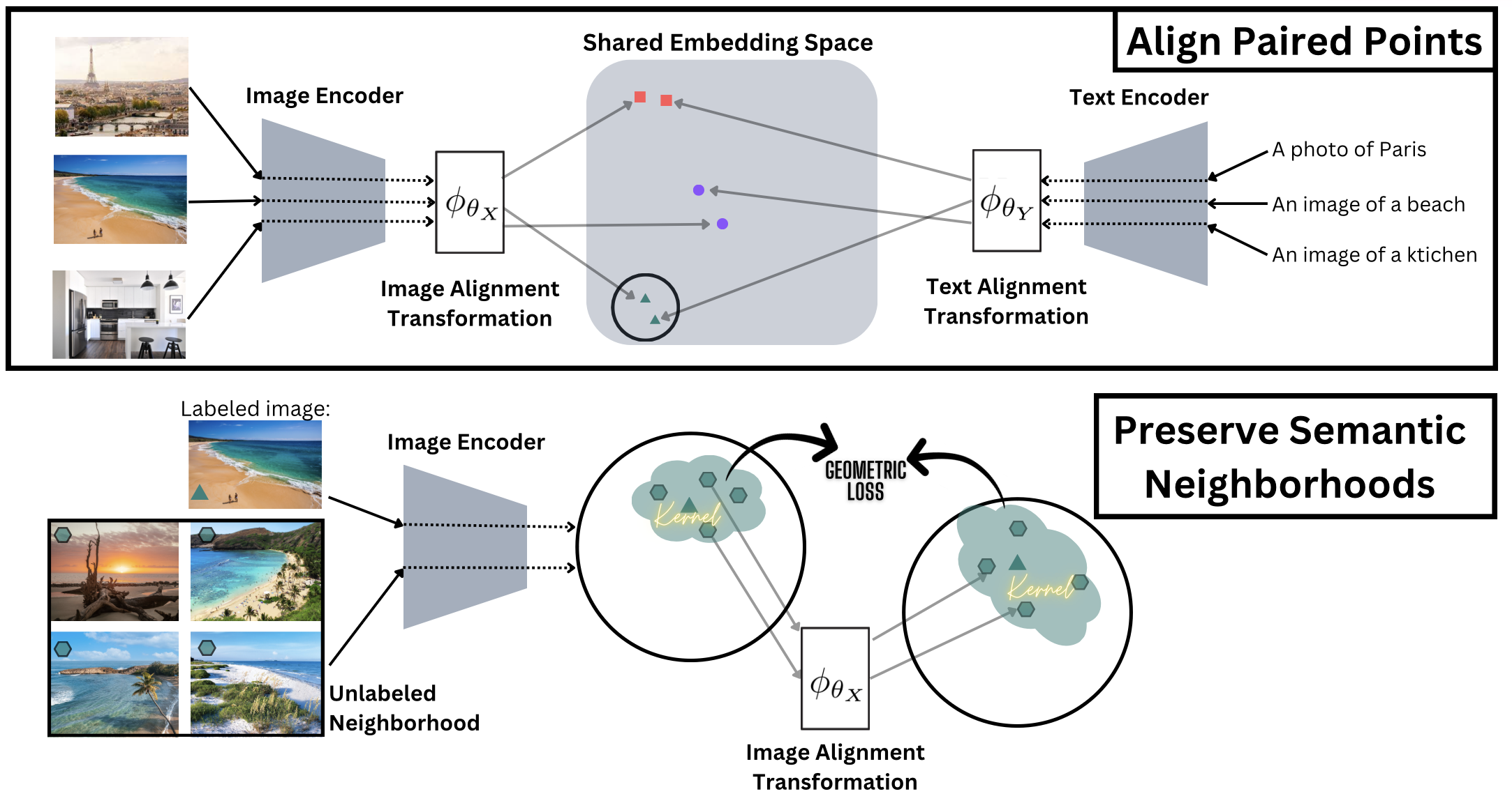
Figure 2: GeRA Training Approach: We optimize image and text alignment functions, focusing on achieving both global alignment of paired points and the preservation of local geometric structures.

2 Related Work

Various multi-modal alignment methods have been introduced, each based on different assumptions about data availability and computational needs; most methods have been applied to align text and image modalities.

Training Multi-Modal Encoders: Radford et al. (2021); Chen et al. (2022); Jia et al. (2021) jointly train image and text encoders from scratch, learning a shared representation for both modalities using a contrastive objective (Wang & Isola, 2020). This approach outperforms many existing models (Kolesnikov et al., 2020; Chen et al., 2020; He et al., 2016) in zero-shot classification on ImageNet (Deng et al., 2009), demonstrating its robust and informative representations. These methods, however, demand large training datasets (Gadre et al., 2023; Thomee et al., 2016; Sun et al., 2017) and consume significant computational resources. Zhai et al. (2021) reduce computational costs by freezing the image encoder and training only the language encoder. While this method enhances performance, it requires an even larger dataset (Sun et al., 2017; Thomee et al., 2016) and remains computationally intensive.

Relative and Anchor-based Encodings: Moschella et al. (2023); Antonello et al. (2021) demonstrate that high-quality encoders produce semantically rich and consistent manifold structures. This observation suggests the concept of relative encodings, where a sample is encoded based on its neighborhood. Such relative encodings have been shown to remain consistent across various encoders and modalities (Moschella et al., 2023). Building on this idea, Norelli et al. (2022) ensure consistent encodings across different modalities using frozen pretrained encoders (Song et al., 2020; Dosovitskiy et al., 2020), eliminating the need for a training phase. Their method achieves high performance, coming close to models trained with substantially more data. However, a trade-off arises: inference time increases with the number of anchor points (labeled data) used.

Unsupervised Alignment Techniques: There has been also research efforts towards unsupervised alignment of embedding spaces without relying on paired modality data. The study Alvarez-Melis & Jaakkola (2018) uses the Gromov-Wasserstein optimal transport objective (Nekrashevich et al., 2023) to align word embeddings from various languages. Despite its advantage of not requiring labeled data, the method poorly scales to the 4th power in terms of the number of embedding points.

Manifold Geometry: Early works in manifold learning, such as Locally Linear Embedding (LLE) (Roweis & Saul, 2000), Isomap (Tenenbaum et al., 2000), and multi-dimensional scaling (Saeed et al., 2018), capture geometric properties of data manifolds while mapping them into simpler spaces. These methods leverage the rich local structure of datasets, constructing a lower-dimensional embedding that retains the topological and geometric characteristics of local neighborhoods in high-dimensional data space.

3 Problem Formulation

3.1 Multi-Modal Alignment

Consider two datasets $X\in\mathbb{R}^{N_{X}\times d_{X}}$ and $Y\in\mathbb{R}^{N_{Y}\times d_{Y}}$, originating from two distinct modalities. Here, $N_{X}$ and $N_{Y}$ denote the number of samples in each dataset, and $d_{X}$ and $d_{Y}$ represent the dimensions of $X$ and $Y$, respectively, which may differ. These datasets denote points embedded by pretrained unimodal encoders. We assume pairwise correspondence for only a small subset of these points, denoted by $\{(x_{p_{i}},y_{q_{i}})\}_{i=1}^{M}$, where $x_{p_{i}}\in X$, $y_{q_{i}}\in Y$, $p_{i}\in[1,N_{X}]$ and $q_{i}\in[1,N_{Y}]$ are some index permutations, and $M\ll N_{X},N_{Y}$. Those pairings correspond to the same objects captured by different modalities. All other points in $X$ and $Y$ are unpaired (unlabeled).

The task at hand is to align the data distributions into a common embedding space. While most methods focus only on aligning the paired data points, we propose to leverage unlabeled (unpaired) points from each modality to preserve the rich geometric structure of their original embedding spaces.

To approach this problem, we define two trainable alignment functions, namely $\phi_{\theta_{X}}:\mathbb{R}^{d_{X}}\rightarrow\mathbb{R}^{d}$ and $\phi_{\theta_{Y}}:\mathbb{R}^{d_{Y}}\rightarrow\mathbb{R}^{d}$, where $d$ is the dimension of the joint embedding space. These alignment transformations are modeled as neural networks. This approach is encoder and modality agnostic, requiring some pretrained unimodal encoder for each modality and a small paird dataset.

3.2 Preserving Manifold Geometry

Unimodal encoders, trained on large and often self-supervised datasets, learn to encode the data into a rich representation that accurately reflects the intrinsic structure of the data. When training the alignment using a smaller paired dataset, this manifold structure might be distorted, degrading the quality of the alignment. Existing methods are not required to preserve these structures, leaving a potential source of information unused. Specifically, learning an alignment using only a contrastive objective, as explored by (Radford et al., 2021), distorts the neighborhood geometry (see Figure 1(b)) and requires substantial paired data to learn an effective alignment.

We propose a geometrically regularized alignment that aligns the paired points while preserving local neighborhood structures, which is motivated by the relation between local neighborhoods and the (Riemannian) manifold geometry (e.g. in approximating geodesic distances) (Coifman & Lafon, 2006; Li & Dunson, 2019). This approach offers global flexibility for obtaining a meaningful alignment and local regularization to maintain the neighborhood structure. The geometry regularization pursues an intuitive goal of keeping similar objects close in the aligned space. This allows for more effective generalization of the learned alignment to nearby (unpaired) points, as evident from the improved performance by our approach (see Section 5.3.) For preserving local neighborhoods, unlabeled data can be leveraged, thus allowing a semi-supervised approach.

4 Geometrically Regularized Alignment Method

4.1 GeRA Loss Function

We introduce the GeRA loss, which optimizes for both aligning paired points and preserving the neighborhood structure of nearby unpaired points. This loss is semi-supervised, as it uses paired data for the alignment and captures the local geometry using both paired and unpaired data. The loss is defined as follows:

$$\mathcal{L}_{GeRA}(\theta_{X},\theta_{Y})=\mathbb{E}_{(X_{B},Y_{B})\sim P_{\text{Pos}}} \Big{[}\underbrace{\mathcal{L}_{Con}(X_{B},Y_{B};\theta_{X},\theta_{Y})+\mathcal{L}_{Con}(Y_{B},X_{B};\theta_{Y},\theta_{X})}_{\text{Alignment}}$$ (1)

$$+\quad\underbrace{\alpha\cdot\big{(}\mathcal{L}_{Geo}(X_{B};\theta_{X})+\mathcal{L}_{Geo}(Y_{B};\theta_{Y})\big{)}}_{\text{Geometric Regularization}}\Big{]}$$

where $\theta_{X}$ and $\theta_{Y}$ parameterize the alignment transformations, $\phi_{\theta_{X}}$ and $\phi_{\theta_{Y}}$, respectively, $P_{Pos}$ represents the uniform distribution over all paired points from both modalities, and $B$ represents the number of paired data points in a batch.

Alignment: We align the labeled points via a contrastive loss, denoted by $\mathcal{L}_{Con}(X_{B},Y_{B};\theta_{X},\theta_{Y})$ as proposed by Radford et al. (2021). It minimizes the distance between positive pairs (paired points) while maximizing the distance of negative samples. We apply this loss to the alignment transformation outputs:

$$\mathcal{L}_{Con}(X_{B},Y_{B};\theta_{X},\theta_{Y}) =-\frac{1}{2}\sum_{x\in X_{B}}\log\frac{\exp\big{(}\text{cossim}(\phi_{\theta_{X}}(x),\phi_{\theta_{Y}}(y))/t\big{)}}{\sum_{y\in Y_{B}}\exp\big{(}\text{cossim}(\phi_{\theta_{X}}(x),\phi_{\theta_{Y}}(y))/t\big{)}}$$ (2)

where $t$ is a temperature hyperparameter.

Geometric Regularization: Our geometric loss term aims to preserve the local geometric structure:

$$\mathcal{L}_{Geo}\left(X_{B};\theta_{X}\right) = \frac{1}{B}\sum_{x\in X_{B}}\mathbb{E}_{\mathrm{N}_{K}(x)\sim S(x)}\Big{[}\left\|\mathbf{W}_{\mathrm{N}_{K}(x)}-\mathbf{W}_{\phi_{\theta_{X}}\left(\mathrm{N}_{K}(x)\right)}\right\|_{F}^{2}\Big{]}.$$ (3)

where $\mathbf{W}_{\mathrm{N}_{K}(x)}$ and $\mathbf{W}_{\phi_{\theta_{X}}\left(\mathrm{N}_{K}(x)\right)}$ are some matrices encoding the neighborhood structure of sample $x$, and $N_{K}(x)$ denotes a sampled set of $K$ neighbors of $x$ (according to the original embedded space). This loss operates only within a single modality and is independent of the other modality. For a given batch of unimodal samples $X_{B}$, we sample a set of $K$ neighbors $N_{K}(x)$, for each sample in the batch, drawn from a precomputed larger neighborhood distribution $S(x)$. We investigate various sampling methods:

• The “closest” method deterministically takes the $K$ nearest neighbors.

• The “uniform” method samples $K$ neighbors uniformly from the larger neighborhood.

• The “biased” method samples proximate neighbors with higher probability than distant neighbors.

The loss in equation 3, penalizes local distortion during the alignment, thus preserving the geometry. The choice of a suitable neighborhood encoding to capture local structure is a crucial consideration. We propose to use an approximation of the heat kernel, discussed in Section 4.2.1. Additionally, we report alternative choices and evaluate the differences in performance in Section 5.5.

4.2 Kernel Encodings

Adding detail to the generic strategy outlined above, we next present the different choices of kernels to encode the neighborhood structure.

4.2.1 The Heat Kernel

Given a set of points, $\{x_{i}\}_{i=1}^{N}$, assumed to lie on some low dimensional manifold, $\mathcal{X}$, the diffusion operator (Coifman & Lafon, 2006), denoted by $\mathbf{W}^{\mathrm{Heat}}$, is defined by:

$$\mathbf{K}^{\mathrm{Heat}}(x_{i},x_{j}) = e^{-\|x_{i}-x_{j}\|_{2}^{2}/4\epsilon}$$

$$\mathbf{W}^{\mathrm{Heat}}(x_{i},x_{j}) = \frac{\mathbf{K}^{\mathrm{Heat}}(x_{i},x_{j})}{\sum_{l}\mathbf{K}^{\mathrm{Heat}}(x_{i},x_{l})}$$ (4)

This operator was shown to converge pointwise to the Neumann heat kernel of the underlying data manifold as $\epsilon$ approaches zero and the number of points tends to infinity. Below, we articulate some advantages of using $\mathbf{W}^{\mathrm{Heat}}$ in our formalism:

Intrinsic. The heat kernel and its approximation are intrinsic, meaning that they are independent of the choice of coordinates. As a result, they are invariant to isometric transformations.

Informative. The heat kernel captures essential intrinsic geometric information. For example, the geodesic distance $g$ between two points $x,y$ on a manifold can be recovered from the heat kernel via the limit (Varadhan, 1967):

$$g(x,y)=\lim_{t\xrightarrow{}0}\sqrt{-4t\log h_{t}(x,y)},$$

where $h_{t}(x,y)$ denotes the continuous heat kernel, which relates to $\mathbf{W}^{\mathrm{Heat}}$ by $h_{t}=\lim_{\epsilon\rightarrow 0,N\rightarrow\infty}(\mathbf{W}^{\mathrm{Heat}})^{t/\epsilon}$ (under slightly different normalization) (Coifman & Lafon, 2006).

Multi-Scale. The locality of the heat kernel is sensitive to the time variable, $t$. In its discrete approximation, $\mathbf{W}^{\mathrm{Heat}}$, the locality is governed by the kernel scale, $\epsilon$, and the sample density of the point cloud. Through these parameters, the heat kernel and its approximation are capable of capturing multi-scale features. Specifically, a smaller $\epsilon$ in equation 4 results in a more local kernel.

4.2.2 Alternative Kernel Encodings

The majority of our experiments use the diffusion operator to capture local neighborhood geometry, but other choices are possible. For example, the following kernels capture the pairwise $L^{2}$ distance and related values:

$$\mathbf{K}^{\mathrm{Linear}}(x_{i},x_{j}) = \|x_{i}-x_{j}\|_{2}\ \ \ \forall x_{i},x_{j}\in X$$ (5)

$$\mathbf{K}^{\mathrm{Squared}}(x_{i},x_{j}) = \|x_{i}-x_{j}\|^{2}_{2}\ \ \ \forall x_{i},x_{j}\in X$$ (6)

$$\mathbf{K}^{\mathrm{Inverse}}(x_{i},x_{j}) = \frac{1}{1+\|x_{i}-x_{j}\|^{2}_{2}}\ \ \ \forall x_{i},x_{j}\in X$$ (7)

We normalize each kernel by the average column values, similarly to the diffusion operator, resulting in the neighborhood encoding $\mathbf{W}^{Z}_{X}$, where $Z$ stands for “Linear”, “Squared” or “Inverse”:

$$\mathbf{W}^{Z}(x_{i},x_{j})=\frac{\mathbf{K}^{Z}(x_{i},x_{j})}{\sum_{l}\mathbf{K}^{Z}(x_{i},x_{l})}$$ (8)

In Section 5.5, we empirically demonstrate that the heat kernel yields the best performance, indicating better preservation of local neighborhood information.

5 Experiments

5.1 Experimental Details

We conduct extensive experiments to show the performance of GeRA under limited data availability with images and text. In addition, in Section 5.4 we present results with speech and text.

Our default experimental setup is adapted from the setup used in ASIF (Norelli et al., 2022), which serves as a baseline.

Dataset: Our training dataset for the image and text experiments is the Conceptual 12M (CC12M) dataset (Changpinyo et al., 2021). This dataset consists of 12 million paired entries of images and their corresponding textual descriptions, spanning a broad spectrum of visual concepts.

Encoders: Two encoders were selected for our first experiments: the Vision Transformer (ViT) (Dosovitskiy et al., 2020) and the Masked and Permuted Network (MPNet) (Song et al., 2020). The base model of the Vision Transformer has 86 million parameters. This model was pretrained on several datasets, including ImageNet-21k and JFT-300M, using the masked patch prediction objective. The base model of MPNet has 109 million parameters. It was pretrained on a large 160GB text corpora, leveraging both masked language modeling and permuted language modeling objectives.

Zero-Shot Accuracy Metric: We use zero-shot accuracy (Xia et al., 2023) as the metric to assess the quality of our alignment method, measured on the well-established ImageNet dataset (Deng et al., 2009). The ImageNet dataset has 1,000 classes, each class is represented by 50 images in the evaluation split. As in Radford et al. (2021), we encode the class names using various prompts and average them in the shared embedding space. The images are directly mapped into the common embedding space using the pretrained encoder together with the subsequent alignment transformation. We calculate the proximity between the image embeddings and each of the 1,000 class embedding vectors using cosine similarity. Image classification is determined by computing the nearest class within the embedding space. Clearly, as the alignment method improves, the zero-shot accuracy increases.

Precision@$k$ Metric: For evaluation beyond image-text alignment we use the Precision@$k$ metric, applied to the test split of the same dataset used for training. We select 10,000 test pairs resulting in 10,000 classes, such that the samples from one modality form classes, and we attempt their retrieval based on corresponding samples of the other modality, and vice versa. Our findings are reported in terms of precision@1 and precision@5. The test samples remain consistent across all experiments.

5.2 Baselines

We verify the effectiveness of our proposed method by comparing it to established baseline models. First, we examine the Procrustes alignment method, which is designed to learn a rotation matrix that aligns one embedding with another. Then, we assess the performance of our alignment transformation functions when trained solely with the contrastive loss, without including our geometry-preserving regularization method. Lastly, we provide a comparison with the ASIF method, as detailed in the related work section.

5.3 Image and Text Alignment through GeRA

5.3.1 Benchmarking on ImageNet and CC12M

We test GeRA with a neighborhood size of $K=150$, using the heat kernel approximation as the neighborhood encoding scheme, and with the “biased” sampling method. We evaluate our performance compared to the baseline methods on the default configuration as described in section 5.1.

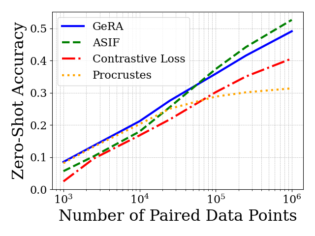
Figure 3: GeRA performance evaluated at zero-shot accruacy on ImageNet against the baselines.

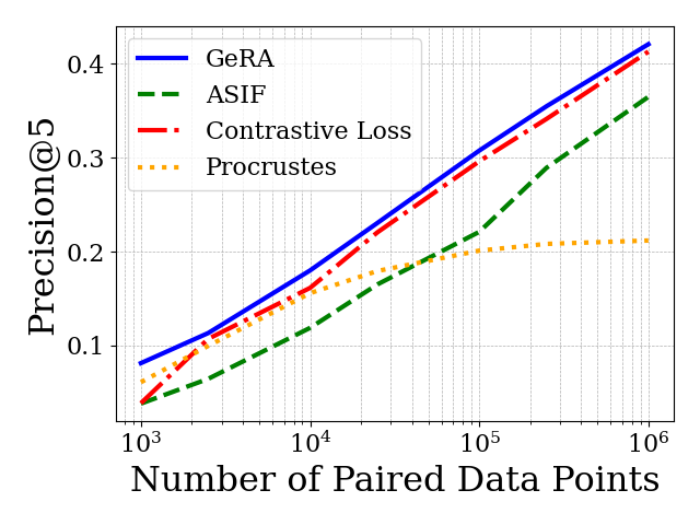
Figure 4: GeRA performance evaluated at precision@5 on in-distribution CC12M data against the baselines.

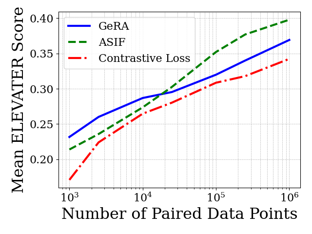
Figure 5: Comparison using mean scores of GeRA, non-regularized method, and ASIF across 20 ELEVATER datasets.

Results: Figure 5 shows that GeRA consistently outperforms both Procrustes Alignment and the unregularized alignment based on the contrastive loss. This validates GeRA’s design choice of balancing local preservation of geometric structures with global flexibility in the alignment process. GeRA demonstrates a significant improvement of almost 9% over the unregularized alignment. The increase in performance is particularly notable in situations where data availability is highly limited, where accuracy improves from 3% for the contrastive loss trained with 1000 samples to almost 9%.

Figure 5 depicts that GeRA is the best-performing model in the low-data regimes. As the volume of data increases, ASIF slightly outperforms GeRA. However, in Figure 5, GeRA exhibits better results when evaluated on precision@5. In Section 5.7, we further demonstrate the advantage of GeRA over ASIF, in terms of inference time.

5.3.2 Benchmarking on ELEVATER

To further validate the generality of our method, we expand our experiments beyond ImageNet and CC12M, incorporating multiple vision-language datasets into our evaluation pipeline. We employed the ELEVATER (Li et al., 2022) benchmark, which contains 20 image classification datasets. These datasets cover a broad spectrum of visual concepts, each presenting varying levels of difficulty.

Results: Figure 5 demonstrates that GeRA consistently outperforms the non-regularized method on the ELEVATER benchmark. In low-data regimes, the benefits of geometric regularization become especially clear. With 1,000 training pairs, the performance gain exceeds 5%. Even with 1 million training pairs, GeRA delivers an average performance improvement of 2.7%. Considering the diverse visual concepts covered in the 20 datasets, it becomes clear that GeRA has superior generalization capabilities.

Compared to ASIF, GeRA demonstrates superior performance in low-data regimes. When trained with 2,500 paired points, GeRA yields a mean score that is almost 3% higher. The advantage of GeRA diminishes as the number of paired points increases; ASIF surpasses GeRA when more paired points are available in training. Specifically, when trained with 1,000,000 paired points, ASIF achieves a mean score 3% higher than GeRA’s. However, in this regime, ASIF is more than $100\times$ slower at inference time, as demonstrated in Figure 9.

5.4 Speech and Text Alignment through GeRA

To further validate adaptability and performance across diverse modalities, we consider the domain of speech-text alignment. We show that our method’s efficacy is not confined to a specific modality and that our hyperparameter choices, optimized for the image-text scenario, are not overfit to that context.

Encoder: We use Whisper (Radford et al., 2023) as the speech encoder consisting of 74 million parameters. For text, we again use MPNet (see Section 5.1).

Dataset: Our training uses the LibriTTS dataset (Zen et al., 2019). This dataset is an assembly of text-speech pairs, aggregating to 585 hours of read English speech. Each entry corresponds to distinct sentences of speech and their textual counterparts. Entries with significant background noise are filtered out. The dataset includes 205,044 pairs in totals, which is considerably smaller than the text-image alignment dataset of 12 million pairs.

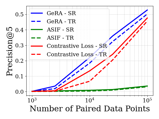
Figure 6: Performance of GeRA compared to ASIF and the pure contrastive learning evaluated at precision@5 for the speech and text alignment, using in-distribution LibriTTS data.

Results: Figure 6 shows that GeRA significantly outperforms ASIF on speech–text alignment. The discrepency increases as the number of paired training points increases With 100,000 training pairs, GeRA achieves a precision@5 score for speech retrieval (SR) of over 51% while ASIF’s score is below 5%. These results show the generalizing capabilities of GeRA to the speech-text domain, while ASIF struggles with this modality. In addition, GeRA surpasses the model trained solely with the contrastive loss, which attains a precision@5 score of 48% for speech retrieval for 100,000 paired training points.

5.5 Influence of Geometry Preservation

We analyze the influence of geometric regularization on GeRA via ablation studies measuring the impact of various design choices. These choices include the size of the neighborhood kernel, the kernel encodings, and the neighborhood sampling method.

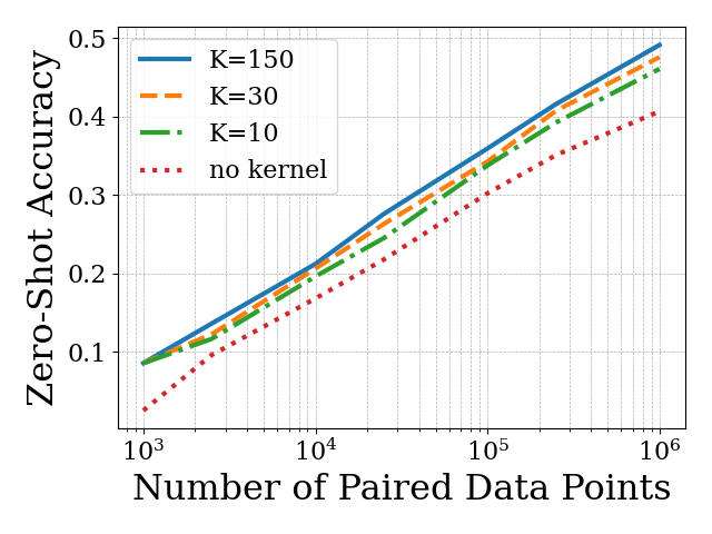
Neighborhood Size

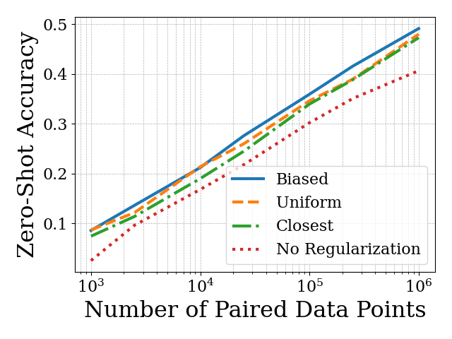
Neighborhood Sampling

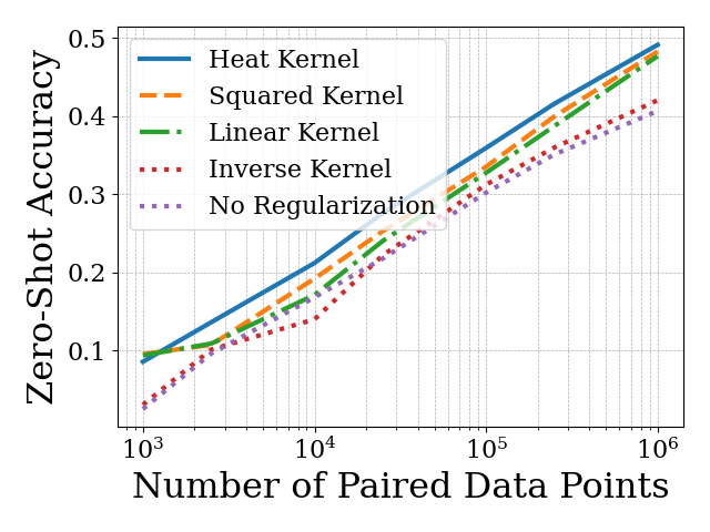
Neighborhood Encodings

Figure 7: The impact of various design choices in GeRA, including neighborhood kernel size, geometry encoding scheme, and neighborhood sampling method.

5.5.1 Results

Neighborhood Size: As the kernel matrix size increases, performance improves, but with diminishing returns. Initial increases in neighborhood size yield substantial gains, but this increase plateaus as the size continues to grow, yielding a trade-off between accuracy and computational cost. We achieve a zero-shot accuracy of over 49% when trained on 1,000,000 paired points using a neighborhood size of 150. Comparing unregularized baseline model to GeRA with a kernel matrix of size 150 yields a 9% increase in top-1 accuracy.

Neighborhood Sampling: Our experiments show that the sampling method affects accuracy. Biased sampling, using primarily close but also including distant neighbors, proves most effective. The uniform distribution ranks second, including equally close and distant neighbors, whereas the least effective sampling method is the “closest” method, which only includes the nearest neighbors All methods surpass the neighborhood-free baseline.

Neighborhood Encoding: Regularization with any of our neighborhood encodings performs better than the contrastive loss alone. Among all, the heat kernel encoding consistently outperforms the other encodings by 2% on average over all training sizes, echoing the theoretical properties inspiring its choice. Overall, our choice of the heat kernel is confirmed to capture geometric information and demonstrates the benefit of geometric regularization in alignment tasks with limited paired data.

5.6 Influence of Pretrained Encoders

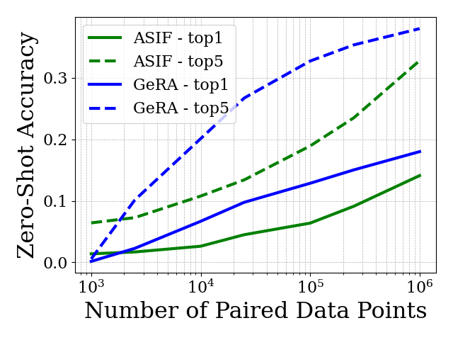
ViT and BERT

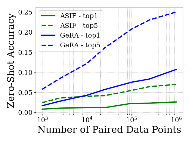
ViT and SentenceTransformer Bert

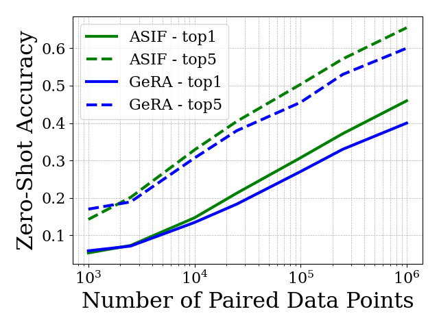
MAE and MPNet

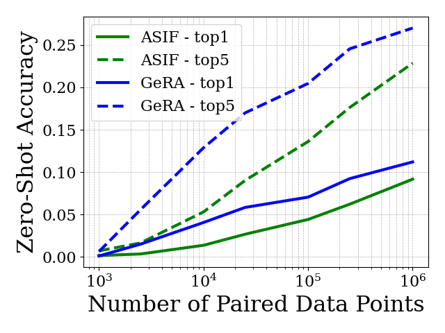
ViT and MPNet

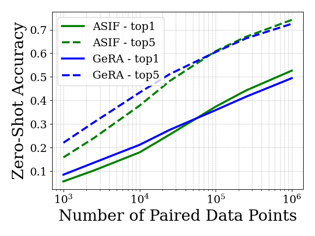
CLIP Encoders

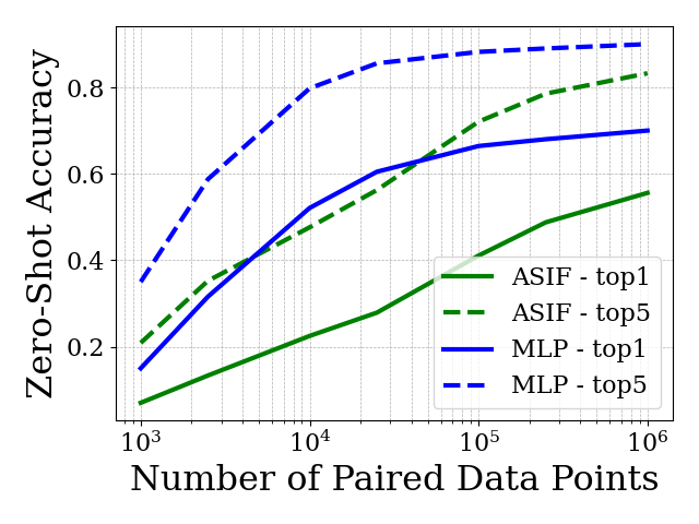
Figure 10: Performance comparison of GeRA and ASIF using various vision and language encoders.

GeRA is encoder-agnostic and hence not tied to a specific choice of encoders. We initially adopted the configurations that were previously tested with ASIF. Next, we discuss the generality of GeRA across different encoders, demonstrated empirically. See results in Figure 10 in the Appendix.

Results: Our method frequently surpasses ASIF by a significant margin with different encoders. This includes CLIP Encoders, the combinations of ViT-RoBERTa, ViT-BERT, and MAE-MPNet. In the configurations recommended by ASIF, however, namely ViT-MPNet or in the setting using ViT-SentenceTransformer BERT, our performance is either on par with or slightly below that of ASIF. Overall, our method offers more consistent and stable results compared to ASIF.

5.7 Training and Inference Time

In Figure 9, GeRA’s training time increases with the neighborhood size used for geometric regularization. Even with the highest number of paired training points (1 million pairs) and the largest kernel size ($K=150$), however, training GeRA on an NVIDIA GeForce RTX 3090 only takes 20 hours. Figure 9 shows that GeRA has consistent inference times, as the alignment transformation during inference is not affected by neighborhood size or number of training pairs. Conversely, ASIF has significant overhead, with inference times increasing linearly in the number of anchor points. For example, with 1 million training pairs, one ASIF inference takes over 2 hours for the retrieval task, while GeRA completes in under 16 seconds.

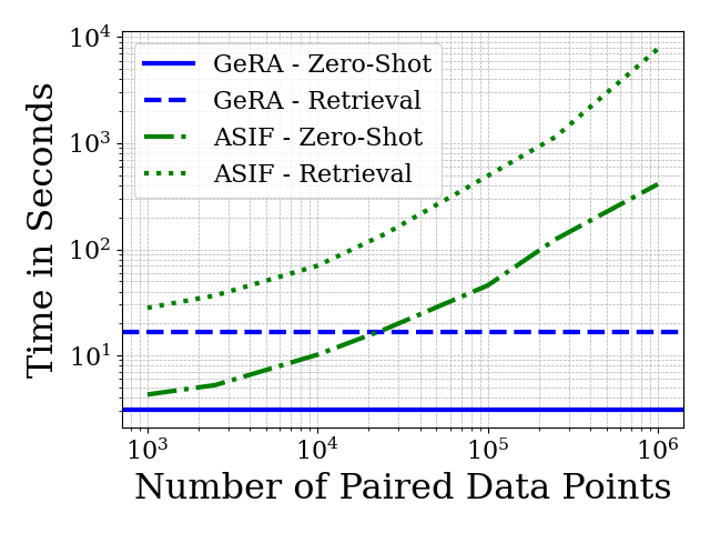
Figure 8: Comparison of inference times between GeRA and ASIF for the Zero-Shot and the Retrieval Evaluation.

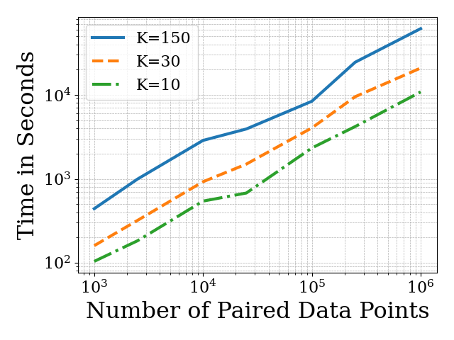
Figure 9: Time for training GeRA with different neighborhood sizes using an NVIDIA GeForce RTX 3090.

6 Discussion

Limitations: Preserving local geometry requires taking neighborhood information into account, which leads to quickly increasing batch sizes, i.e., for batch size $B$ and geometric regularization with $K$ neighbors, the effective batch size becomes $B\cdot K$. This limits the ability to use larger batch sizes, which may slow down the convergence.

Moreover, GeRA depends on powerful pretrained models that define the geometry. In the absence of powerful pretrained models, the regularization’s effectiveness diminishes. Our experiments in section 5.6 show that selecting powerful encoders are necessary for both GeRA and ASIF. One potential solution in the absence of powerful pretrained encoders is to collect corrected neighborhood information for our loss term using human annotations or rules defined by a domain expert.

Future Work: Our work opens several interesting future work directions. In terms of the attractive capability of GeRA to align domains with limited paired data supervision, there are several other modalities and downstream tasks that could be explored. Examples include aligning protein sequences and biomedical texts, which is needed for protein representation learning. Traditional unimodal approaches, which only focus on protein sequences, often miss functional aspects of proteins. Recent efforts incorporate text data on protein functions as an additional modality, enriching representations (Xu et al., 2023). However, the available datasets are relatively small, featuring only half a million paired data points. As a result, this domain is a key target for future work on GeRA. Additional future work directions for GeRA include exploring learnable parametric geometric kernels (e.g. realized as self-attention blocks or small transformers), simultaneous co-training and multi-task training of both the encoders (on the uni-modal data components) and the GeRA alignment module leading to dynamically changing manifolds landscape and potentially requiring exploring into momentum models for increased training stability, exploring multi-scale (coarsening, multi-grid) manifold mapping methods to further enhance the preservation of the more global manifold structure after alignment, and many more.

7 Acknowledgement

The MIT Geometric Data Processing group acknowledges the generous support of Army Research Office grants W911NF2010168 and W911NF2110293, of Air Force Office of Scientific Research award FA9550-19-1-031, of National Science Foundation grants IIS-1838071 and CHS-1955697, from the CSAIL Systems that Learn program, from the MIT–IBM Watson AI Laboratory, from the Toyota–CSAIL Joint Research Center, from a gift from Adobe Systems, and from a Google Research Scholar award.

Appendix A Appendix

A.1 Experimental Details - Hyperparameters

Table 1: Summary of the explored hyperparameter spaces and the optimal values discovered for each method. The table outlines the range of values over which each hyperparameter was tuned, denoted in the ‘Range’ column. Subsequent columns present the hyperparameter values that yielded the best performance for each respective method, GeRA, Contrastive Loss, and ASIF (hyperparameters as stated in the paper (Norelli et al., 2022)), during experimentation. In instances where a hyperparameter is not applicable to a method, the cell is left blank.

Hyperparameter	Range	GeRA	Contrastive Loss	ASIF
Batch Size	500-4,000	2000	2000	–
Learning Rate	1e-5 – 5e-4	2e-4	2e-4	–
Dropout	0.0 – 0.5	0.3	0.3	–
Number of Hidden Layers	1 – 3	1	1	–
Hidden Dimension	768 – 16,000	8000	8000	–
Output Dimension	512 – 768	768	768	–
Neighborhood Size	5 – 150	150	–	–
Alpha	0.1 – 2.0	0.5	–	–
Epsilon	0.1 – 3.0	0.8	–	–
Temperature	0.01 – 0.4	0.04	0.04	–
p (Exponentiation)	1 – 8	–	–	8
k (Sparsification)	50 – 1600	–	–	800

Alpha: This parameter balances the geometric regularization term with the contrastive objective, determining the relative importance of each in the loss function (See Equation 1).

Epsilon: This represents the kernel size, influencing the locality of the kernel matrix. A smaller epsilon value implies that the heat kernel captures more localized features, thereby considering neighbors in closer proximity (See Equation 4).

Temperature: Applied in the output layer, the temperature parameter modulates the sharpness of the distribution. A higher temperature results in a softer probability distribution over classes, whereas a lower temperature makes the distribution more concentrated (See Equation 2).

Neighborhood Size: This parameter specifies the number of neighbors included into the geometric regularization loss (see Equation 3).

A.2 Evaluating GeRA on different Pretrained Encoders

ViT and RoBERTa

References

- Alvarez-Melis & Jaakkola (2018) David Alvarez-Melis and Tommi S. Jaakkola. Gromov-wasserstein alignment of word embedding spaces. CoRR, abs/1809.00013, 2018. URL http://arxiv.org/abs/1809.00013.
- Antonello et al. (2021) Richard Antonello, Javier S Turek, Vy Vo, and Alexander Huth. Low-dimensional structure in the space of language representations is reflected in brain responses. Advances in neural information processing systems, 34:8332–8344, 2021.
- Baltrušaitis et al. (2018) Tadas Baltrušaitis, Chaitanya Ahuja, and Louis-Philippe Morency. Multimodal machine learning: A survey and taxonomy. IEEE transactions on pattern analysis and machine intelligence, 41(2):423–443, 2018.
- Changpinyo et al. (2021) Soravit Changpinyo, Piyush Sharma, Nan Ding, and Radu Soricut. Conceptual 12m: Pushing web-scale image-text pre-training to recognize long-tail visual concepts. In Proceedings of the IEEE/CVF Conference on Computer Vision and Pattern Recognition, pp. 3558–3568, 2021.
- Chen et al. (2020) Ting Chen, Simon Kornblith, Kevin Swersky, Mohammad Norouzi, and Geoffrey E Hinton. Big self-supervised models are strong semi-supervised learners. Advances in neural information processing systems, 33:22243–22255, 2020.
- Chen et al. (2022) Zhongzhi Chen, Guang Liu, Bo-Wen Zhang, Fulong Ye, Qinghong Yang, and Ledell Wu. Altclip: Altering the language encoder in clip for extended language capabilities. arXiv preprint arXiv:2211.06679, 2022.
- Coifman & Lafon (2006) Ronald R. Coifman and Stéphane Lafon. Diffusion maps. Applied and Computational Harmonic Analysis, 21(1):5–30, 2006. ISSN 1063-5203. doi: https://doi.org/10.1016/j.acha.2006.04.006. URL https://www.sciencedirect.com/science/article/pii/S1063520306000546. Special Issue: Diffusion Maps and Wavelets.
- Deng et al. (2009) Jia Deng, Wei Dong, Richard Socher, Li-Jia Li, Kai Li, and Li Fei-Fei. Imagenet: A large-scale hierarchical image database. In 2009 IEEE Conference on Computer Vision and Pattern Recognition, pp. 248–255, 2009. doi: 10.1109/CVPR.2009.5206848.
- Dosovitskiy et al. (2020) Alexey Dosovitskiy, Lucas Beyer, Alexander Kolesnikov, Dirk Weissenborn, Xiaohua Zhai, Thomas Unterthiner, Mostafa Dehghani, Matthias Minderer, Georg Heigold, Sylvain Gelly, Jakob Uszkoreit, and Neil Houlsby. An image is worth 16x16 words: Transformers for image recognition at scale. CoRR, abs/2010.11929, 2020. URL https://arxiv.org/abs/2010.11929.
- Gadre et al. (2023) Samir Yitzhak Gadre, Gabriel Ilharco, Alex Fang, Jonathan Hayase, Georgios Smyrnis, Thao Nguyen, Ryan Marten, Mitchell Wortsman, Dhruba Ghosh, Jieyu Zhang, et al. Datacomp: In search of the next generation of multimodal datasets. arXiv preprint arXiv:2304.14108, 2023.
- Gower (1975) John C Gower. Generalized procrustes analysis. Psychometrika, 40:33–51, 1975.
- He et al. (2016) Kaiming He, Xiangyu Zhang, Shaoqing Ren, and Jian Sun. Deep residual learning for image recognition. In Proceedings of the IEEE conference on computer vision and pattern recognition, pp. 770–778, 2016.
- Jia et al. (2021) Chao Jia, Yinfei Yang, Ye Xia, Yi-Ting Chen, Zarana Parekh, Hieu Pham, Quoc Le, Yun-Hsuan Sung, Zhen Li, and Tom Duerig. Scaling up visual and vision-language representation learning with noisy text supervision. In International conference on machine learning, pp. 4904–4916. PMLR, 2021.
- Kolesnikov et al. (2020) Alexander Kolesnikov, Lucas Beyer, Xiaohua Zhai, Joan Puigcerver, Jessica Yung, Sylvain Gelly, and Neil Houlsby. Big transfer (bit): General visual representation learning. In Computer Vision–ECCV 2020: 16th European Conference, Glasgow, UK, August 23–28, 2020, Proceedings, Part V 16, pp. 491–507. Springer, 2020.
- Li et al. (2022) Chunyuan Li, Haotian Liu, Liunian Li, Pengchuan Zhang, Jyoti Aneja, Jianwei Yang, Ping Jin, Houdong Hu, Zicheng Liu, Yong Jae Lee, et al. Elevater: A benchmark and toolkit for evaluating language-augmented visual models. Advances in Neural Information Processing Systems, 35:9287–9301, 2022.
- Li & Dunson (2019) Didong Li and David B Dunson. Geodesic distance estimation with spherelets. arXiv preprint arXiv:1907.00296, 2019.
- Moschella et al. (2023) Luca Moschella, Valentino Maiorca, Marco Fumero, Antonio Norelli, Francesco Locatello, and Emanuele Rodolà. Relative representations enable zero-shot latent space communication, 2023.
- Nekrashevich et al. (2023) Maksim Nekrashevich, Alexander Korotin, and Evgeny Burnaev. Neural gromov-wasserstein optimal transport. arXiv preprint arXiv:2303.05978, 2023.
- Norelli et al. (2022) Antonio Norelli, Marco Fumero, Valentino Maiorca, Luca Moschella, Emanuele Rodola, and Francesco Locatello. Asif: Coupled data turns unimodal models to multimodal without training. arXiv preprint arXiv:2210.01738, 2022.
- Radford et al. (2021) Alec Radford, Jong Wook Kim, Chris Hallacy, Aditya Ramesh, Gabriel Goh, Sandhini Agarwal, Girish Sastry, Amanda Askell, Pamela Mishkin, Jack Clark, Gretchen Krueger, and Ilya Sutskever. Learning transferable visual models from natural language supervision. CoRR, abs/2103.00020, 2021. URL https://arxiv.org/abs/2103.00020.
- Radford et al. (2023) Alec Radford, Jong Wook Kim, Tao Xu, Greg Brockman, Christine McLeavey, and Ilya Sutskever. Robust speech recognition via large-scale weak supervision. In International Conference on Machine Learning, pp. 28492–28518. PMLR, 2023.
- Roweis & Saul (2000) S. T. Roweis and L. K. Saul. Nonlinear dimensionality reduction by locally linear embedding. In Science, pp. 2323–2326, 2000.
- Saeed et al. (2018) Nasir Saeed, Haewoon Nam, Mian Imtiaz Ul Haq, and Dost Bhatti Muhammad Saqib. A survey on multidimensional scaling. ACM Computing Surveys (CSUR), 51(3):1–25, 2018.
- Schuhmann et al. (2021) Christoph Schuhmann, Richard Vencu, Romain Beaumont, Robert Kaczmarczyk, Clayton Mullis, Aarush Katta, Theo Coombes, Jenia Jitsev, and Aran Komatsuzaki. Laion-400m: Open dataset of clip-filtered 400 million image-text pairs. arXiv preprint arXiv:2111.02114, 2021.
- Song et al. (2020) Kaitao Song, Xu Tan, Tao Qin, Jianfeng Lu, and Tie-Yan Liu. Mpnet: Masked and permuted pre-training for language understanding. Advances in Neural Information Processing Systems, 33:16857–16867, 2020.
- Sun et al. (2017) Chen Sun, Abhinav Shrivastava, Saurabh Singh, and Abhinav Gupta. Revisiting unreasonable effectiveness of data in deep learning era. In Proceedings of the IEEE international conference on computer vision, pp. 843–852, 2017.
- Tenenbaum et al. (2000) Joshua B Tenenbaum, Vin de Silva, and John C Langford. A global geometric framework for nonlinear dimensionality reduction. science, 290(5500):2319–2323, 2000.
- Thomee et al. (2016) Bart Thomee, David A Shamma, Gerald Friedland, Benjamin Elizalde, Karl Ni, Douglas Poland, Damian Borth, and Li-Jia Li. Yfcc100m: The new data in multimedia research. Communications of the ACM, 59(2):64–73, 2016.
- Varadhan (1967) S. R. S. Varadhan. On the behavior of the fundamental solution of the heat equation with variable coefficients. Communications on Pure and Applied Mathematics, 1967.
- Wang & Isola (2020) Tongzhou Wang and Phillip Isola. Understanding contrastive representation learning through alignment and uniformity on the hypersphere. In International Conference on Machine Learning, pp. 9929–9939. PMLR, 2020.
- Xia et al. (2023) Heming Xia, Qingxiu Dong, Lei Li, Jingjing Xu, Ziwei Qin, and Zhifang Sui. Imagenetvc: Zero-shot visual commonsense evaluation on 1000 imagenet categories. arXiv preprint arXiv:2305.15028, 2023.
- Xu et al. (2023) Minghao Xu, Xinyu Yuan, Santiago Miret, and Jian Tang. Protst: Multi-modality learning of protein sequences and biomedical texts. arXiv preprint arXiv:2301.12040, 2023.
- Zen et al. (2019) Heiga Zen, Viet Dang, Rob Clark, Yu Zhang, Ron J Weiss, Ye Jia, Zhifeng Chen, and Yonghui Wu. Libritts: A corpus derived from librispeech for text-to-speech. arXiv preprint arXiv:1904.02882, 2019.
- Zhai et al. (2021) Xiaohua Zhai, Xiao Wang, Basil Mustafa, Andreas Steiner, Daniel Keysers, Alexander Kolesnikov, and Lucas Beyer. Lit: Zero-shot transfer with locked-image text tuning. CoRR, abs/2111.07991, 2021. URL https://arxiv.org/abs/2111.07991.