Quintessence scalar field model in Weyl-type Gravity with analysis
Vinod Kumar Bhardwaj1, Priyanka Garg2
Department of Mathematics, GLA University, Mathura-281 406,
Uttar Pradesh, India
1E-mail:dr.vinodbhardwaj@gmail.com
2E-mail:pri.19aug@gmail.com
Abstract
In the present study, we explore the dynamical characteristics of the quintessence cosmological model in Weyl-type gravity. Here, represents the trace of the matter energy-momentum tensor, and symbolizes the nonmetricity tensor. We propose a solution to the field equation using the specific parametrization in the form, which depicts the necessary transition of cosmos from decelerating era to the current accelerating scenario. The values of model parameters are estimated as , , and using the MCMC analysis and limiting the model with a joint dataset of Pantheon, BAO, and OHD. We discuss the cosmic behavior of many features of the derived model like EoS parameters, energy density, and cosmic pressure. Further, we have also explored the cosmological behavior of the quintessence model in Weyl gravity. We have described the cosmic behavior of the model by analysis. The diagnosis of the model is also performed using state finders and jerk parameters. In the end, we have discussed the energy conditions for the proposed model. Our analysis shows that the suggested model is well consistent with the recent findings.
Keywords : Weyl-type gravity, Observational constraints, State finders, Quintessence DE model, analysis.
PACS: 98.80.-k
1 Introduction
In the early 20th century, astronomers like Edwin Hubble suggested the idea of expanding the universe when they saw that galaxies were moving apart from one another. But in the late 1990s, supernova experiments added a new unexpected finding in the expansion discovery of the universe which is that the universe was not only expanding, but it was growing faster. Later on, numerous cosmological observations have also confirmed these cosmological findings [1, 2, 3, 4, 5, 6, 7]. To explain this accelerated expansion, scientists proposed the existence of a mysterious form of energy called Dark energy (DE). DE is postulated to have a negative pressure and is associated with the vacuum energy of space itself [8, 9]. This negative pressure leads to the repulsive gravitational effects that drive the universe’s accelerated expansion [10, 11]. Current theories suggest that dark energy constitutes about of the total energy content of the universe. This is the dominant contributor to the total matter of the universe, along with about of dark matter, and the rest in the form of normal matter (atoms).
To explain the cosmic expansion, a term has been introduced in Einstein’s equation as an alternative to DE. This term causing space to repel itself and leading to the observed accelerated expansion is called a cosmological constant. However, this approach faces two major challenges: the problems of fine-tuning and cosmic coincidence. To address these challenges, alternative theories of gravitation have been explored. Modified theories of gravity involve modifying the gravitational part of Einstein’s equations in various ways. These modifications could potentially explain the accelerated expansion. Such theories might provide explanations for the accelerated expansion by altering fundamental laws of gravity rather than invoking a new form of energy. Several theories have been developed through modifications of Lagrangian and curvature of Einstein’s equations in general relativity [12, 13, 14, 15, 16, 17, 18, 19, 20]. Among these modified theories, theory is one of the appropriate alternatives of GR theory, which faces challenges in passing certain observational tests [21, 22, 23, 24, 25, 26, 27]. The theory is another modified version of theory that explains the accelerated expansion of the universe at late times [28, 29, 30, 31, 32].
“ gravity" is an extension of gravity within the field of theoretical physics and cosmology that extends and modifies Einstein’s General Theory of Relativity (GR). In General Relativity, the gravitational interaction between masses is described by the curvature of space-time caused by the distribution of matter and energy. In theory the energy-momentum tensor describes the distribution of matter and energy in space-time, and the quadratic scalar is a mathematical term derived from the geometry of the space-time manifold. By allowing for a wider range of functions and interactions between these two terms, gravity aims to provide a more comprehensive and flexible description of gravitational phenomena. In some gravity models, modifications to the gravitational field equations can lead to predictions that mimic the effects of dark matter and dark energy, thus providing alternative explanations for the observed cosmic acceleration and galactic rotation curves. Researchers and cosmologists are actively exploring various gravity models to better understand their implications for cosmology, astrophysics, and fundamental physics [34, 35, 36]. In the study of the expansion of the current universe, Bhattacharjee et al. [37], and Arora et al. [38] have also focused on the framework of gravity. This approach allows researchers to explore modifications to the standard General Relativity equations and their implications for the evolution of the cosmos. Zia et. Al. [39] discusses the general form of the transient behavior of gravity. This likely includes a study of how this modified gravity theory behaves over time, especially in comparison to standard General Relativity. The reference [40] appears to focus on explaining the parameters of a linear case model within the context of gravity. This kind of study helps establish the relationships between the theory’s parameters and its predictions.
Weyl-type gravity is a fascinating extension of gravitational theory that introduces a novel approach to understanding the fundamental forces governing the universe. In this framework, the traditional Einstein-Hilbert action is modified by incorporating a function of the Weyl tensor () and the trace of the energy-momentum tensor (). This modification allows for a richer description of gravity and space-time geometry. In gravitational physics, the Weyl tensor represents the traceless part of the Riemann curvature tensor. It characterizes the gravitational tidal forces and describes the intrinsic geometry of space-time. The energy-momentum tensor encodes information about the distribution of matter and energy in space-time. Weyl-type gravity is a rapidly evolving field of research. Scientists Yixin et al. [41], Yang et al. [42], Gadbail et al. [43] are actively investigating various models, cosmological implications, and observational tests to validate or refine this framework. In the context of Weyl-type gravity, reference [44] discusses the impact of viscosity on cosmological evolution. This suggests an investigation into how the presence of viscosity affects the dynamics of the universe within the framework of this modified gravity theory. Gadbail et al. [45] have used parametrization of DP to explore the cosmological dynamics of the universe in Weyl-type gravity.
In the present study, we have explored the cosmological dynamics of the universe in Weyl-type by assuming the parametrization . The present study is organized as: In Section , we have discuss the formulation in Weyl-type gravity. Using parametrization of the deceleration parameter, the solution of field equations has been proposed in Section . In Section , we have discussed the observational constraints with Hubble data points in the range . Some features of the proposed model are explained in Section . The viability of the derived model is also examined through in Section . The quintessence field is defined in Section . State-finders and sound speed are explained in Sections and . Classical linear and nonlinear energy conditions are defined in Section . Finally, in Section conclusion is summaries.
2 Field equation of Weyl type gravity
Weyl proposed a new geometry in 1918, that introduces a relationship characterized by the change in both the orientation and magnitude of a vector under parallel vector transport. The formulation of the action in Weyl gravity is defined as [41].
| (1) |
with . Non-metricity Q is an essential aspect of our theory that can be determined through the process.
| (2) |
here is define as
| (3) |
The covariant derivative of metric in the Riemannian geometry is zero but in Weyl geometry, non metricity tensor is defined as
| (4) |
From Eq. (3) and (4), we find the following relation
| (5) |
The generalized equation by variation on Eq.(1) is
| (6) |
The effective mass of the vector field is
| (7) |
The variation on action (1) w.r.t. metric tensor and weyl vector yield
| (8) |
here, and are the partial derivatives of w.r.to and respectively. and are define as
| (9) |
| (10) |
Here, Re-scaled energy momentum tensor is given by
| (11) |
and
| (12) |
The energy-momentum tensor in the weyl gravity is defined as
| (13) |
As a result, the matter energy-momentum tensor is not conserved, meaning that it does not remain constant over time. This non-conservation is indicated by the presence of a non-zero right-hand side in the equation. Physically, the non-conservation of the matter energy-momentum tensor implies the existence of an additional force acting on massive test particles. This force affects the motion of these particles, causing them to be non-geodesic. Geodesic motion refers to the path that a free particle would naturally follow in the absence of any external forces [46].
3 Cosmological model with deceleration parameter
For the purpose of modeling, we consider a spatially flat FLRW metric.
| (14) |
here represents the scale factor. Because of spatial symmetry, the vector field can be assume as . Using this we get,
The energy momentum tensor for the perfect fluid is given by:
| (15) |
here and are energy density and pressure, respectively. is the four velocity vector satisfying . So we have
The generalized Proca equation and constraint of flat space in the cosmological case can be found as:
| (16) |
| (17) |
| (18) |
Using equation (8) and (15), the generalized Friedmann equations define as,
| (19) |
| (20) |
Eliminating the derivatives of from Eqs. (17) (18), (19), and (20), we get following to expressions.
| (21) |
| (22) |
where are the partial derivatives w.r.to and and dot(.) indicates time derivative. In the present study, we assume ; here, and are the parameters. represents the Weyl field’s mass and denotes the strength of coupling between matter and the Weyl geometry. For this case, we assume [41]. It is important to note that for and , Weyl type reduces to a successful reduction of GR. On the other hand, for , it turns to , which is equivalent to GR and is consistent with cosmological assessments and observational findings. Additionally, by utilizing the expression we can obtained .
Now, the following expressions of the pressure and energy density can be determined using Eqs. (21) and (22).
| (23) |
and
| (24) |
We obtain EoS parameter from equations (23) and (24),
| (25) |
Parametric form of Deceleration Parameter
The deceleration parameter, , describes the rate of change of the expansion of the universe. It provides information about the universe’s expansion at a particular point in its history. The deceleration parameter can be used to classify the evolution of the universe into different phases: indicates that the expansion of the universe is decelerating. In other words, the rate of expansion is slowing down over time. This is typical for a universe dominated by matter and radiation. signifies that the universe’s expansion is neither accelerating nor decelerating. It could correspond to a transitional phase between deceleration and acceleration. suggests that the expansion of the universe is accelerating. In this scenario, the rate of expansion is increasing over time. This can be attributed to the presence of dark energy, a hypothetical form of energy with negative pressure that counteracts the gravitational attraction of matter.
The parametric form of Deceleration Parameter (DP) is considered as[47].
| (26) |
here, and are fixed values. The current deceleration parameter value, denoted as equal to , at . Furthermore, for specific value of and , the value of deceleration parameter is equal to which indicate that the universe is dominated by dark matter. In terms of redshift , the Hubble parameter can be defined as:
| (27) |
From Eqs. (26) and (27), we can explain the Hubble parameter as
| (28) |
Here, denotes the current value of the Hubble parameter.
4 Observational data analysis
In this segment, we have applied the Markov Chain Monte Carlo (MCMC) technique to find the best-fitted optimal parameter values of the model. Here, signifies the theoretically predicted value, while stands for the observational value. The evaluation function is examined as follows:
| (29) |
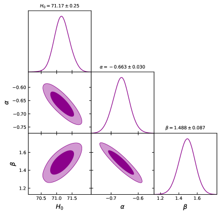
In this context, signifies the parameters of the model, while denotes the standard errors associated with measurements of a physical measure. Here, the parameter vector is denoted by . Through a statistical process that involves minimizing the estimation function , it becomes possible to determine the most probable values of parameters. For this purpose, we utilized the datasets of experimental findings like the observational Hubble data (OHD) consisting of 57points within the range [48, 49], Pantheon dataset of 1048 Type Ia Supernovae (SN Ia) within the redshift range [50], and an observation dataset related to baryon acoustic oscillation (BAO) [51, 52, 53, 54, 55]. The confidence contour plots with () and () confidence in two dimensional for the given model are shown in Figure 1. The summary of best-estimated values of parameters for the derived model are tabulated in Table 1.
| Parameters | |||||
|---|---|---|---|---|---|
| BAO+OHD57+Pantheon | |||||
| BAO+OHD57 | |||||
| Pantheon | |||||
| OHD57 |
For the combined observed data set, the estimator can be expressed as
| (30) |
5 Features of the Model
(a)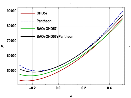 (b)
(b)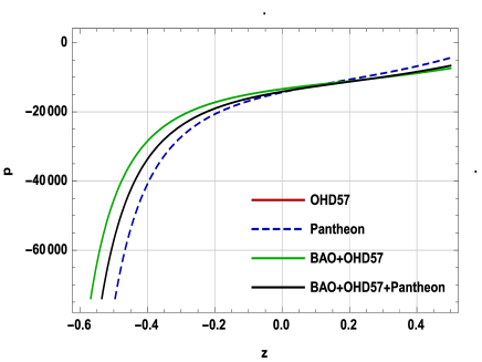
For all observational datasets energy density is positive of Weyl-type of gravity as shown in Figure 2(a). For various observational datasets, the behavior of cosmic pressure is demonstrated in Figure 2(b). It has been seen that the pressure is negative throughout the whole evolution of the universe. The negative behavior describes the present accelerated expansion of the universe. It also explains that with the universe’s development, the energy density diminishes, leading to an increase in the volume of space.
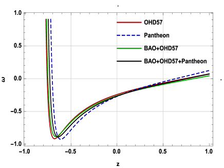
The equation of state parameter is a crucial parameter in cosmology and astrophysics that describes the relationship between the pressure and the energy density of a substance, such as matter or dark energy, in the universe. It is used to characterize the nature of the substance and its effect on the expansion of the universe. The value of the equation of state parameter can vary for different substances: For non-relativistic matter, the pressure is negligible compared to the energy density, so is close to 0. For relativistic particles, such as photons and neutrinos, the pressure is significant compared to the energy density, leading to . This is due to the relativistic equation of state. The equation of state parameter for a cosmological constant is , which means that its pressure is negative and equal in magnitude to its energy density. This negative pressure is responsible for the accelerated expansion of the universe. Some theories propose that dark energy might not be a cosmological constant but instead a dynamic field evolving over time. In these cases, the EoS parameter can vary and be different from -1. It could be greater than -1 (indicating repulsive gravity) or less than -1 (indicating even more rapid expansion). From the figure, we can observed that the derived model initially lies in quintessence era and advanced to Chaplygin gas scenario in late time [56, 61].
6 Analysis
Caldwell and Linder [63] conducted a study to investigate the changing dynamics of quintessence models of dark energy in the phase plane represented by and its time derivative , where is the derivative of with respect to the logarithm of the scale factor i.e. (). They demonstrated that these models classified into two distinct regions in the phase plane, known as the ‘thawing’ () and ‘freezing’ regions () with quite different behavior in the plane [64, 65, 66].
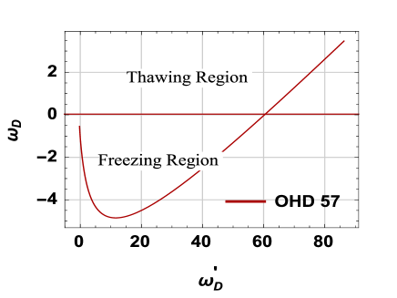
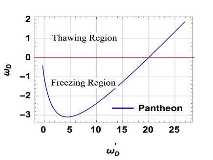
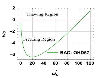
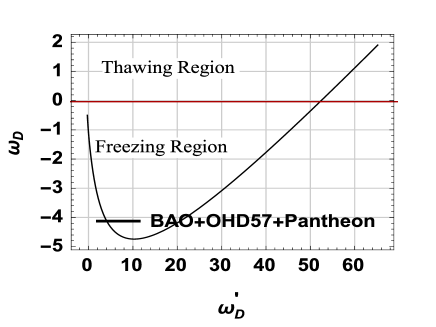
We have plotted against for all the observational values in Figure 4 to construct the plane. The curves in the plot exhibit both freezing and thawing regions for different observational datasets. We observe that our model’s trajectories primarily diverge in the freezing region, as supported by observational data, indicating a more accelerated expansion of the universe in this area.
7 Quintessence field in Weyl-type of gravity
Quintessence is a theoretical concept in cosmology that refers to a hypothetical scalar field responsible for dark energy. It is considered one of the leading explanations for the accelerated expansion of the universe. The term "quintessence" comes from ancient cosmology, where it was used to describe the fifth element that completes the classical four elements of earth, water, air, and fire. In modern cosmology, quintessence is associated with a scalar field that has a positive energy density and negative pressure, causing it to have repulsive gravitational effects. This negative pressure leads to the expansion of the universe at an accelerating rate, counteracting the attractive gravitational force of matter and radiation. The presence of quintessence would help explain the observed phenomenon of DE. The dynamics of the quintessence field depend on its potential energy function. Different potential energy functions result in different behaviors of the quintessence field over cosmic time. The scalar potential is a basic idea in physics, which gives each point in space a unique value to describe the energy associated with a scalar field. The specific physical system under examination will determine the properties of this field and its potential. Since negative energy can lead to solutions that defy the laws of physics, a positive scalar potential is often linked with stable configurations in physics.
The negative scalar potential is demonstrated in specific frameworks like models involving dark energy or cosmological inflation. The behavior of a scalar potential is ultimately determined by physics and the particular values of relevant parameters.
The action for the quintessence field is explained as, [67]
| (31) |
where is the metric determinant is the metric in the above Eq.(31), is the potential for the quintessence field . The energy density and pressure for the quintessence scalar field by varying the action w.r.t. the metric and are defined as:
| (32) |
(a)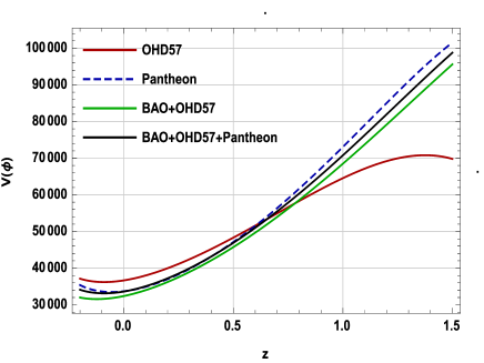 (b)
(b)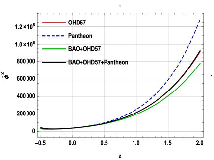
Figures 5(a) and 5(b) illustrate the changes in the scalar field and its corresponding potential within the quintessence model as the redshift z varies. The plots were generated using the estimated values of parameters. For these suitable choices of parameters, the field gets trapped in the local minimum because the kinetic energy during a scaling regime is small. The field then enters a regime of damped oscillations leading to an accelerating universe [61, 67, 68].
8 statefinders
Statefinder is a cosmological diagnostic tool used in astrophysics and cosmology to distinguish between different dark energy (DE) models. It has been computed for various existing models of dark energy, that provide an effect between different forms of dark energy in the cosmological plane. This plane represents distinct, well-known regions of the universe. For instance, the pair and corresponds to the region of quintessence DE eras, represents the CDM limit, signifies the CDM limit, and and ) indicates the Chaplygin gas region. Using this diagnostic tool, one can assess how closely a dark energy model resembles CDM dynamics [69, 70]. Alam et al. [71] have defined the state-finders (, ) as following
| (33) |
where is the scale factor of the universe, H is the Hubble parameter, and the primes represent derivatives with respect to the cosmic time. State-finder depends on the scale factor and its time derivative. The state-finders can also read as
| (34) |
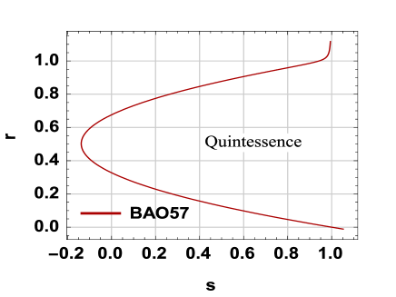
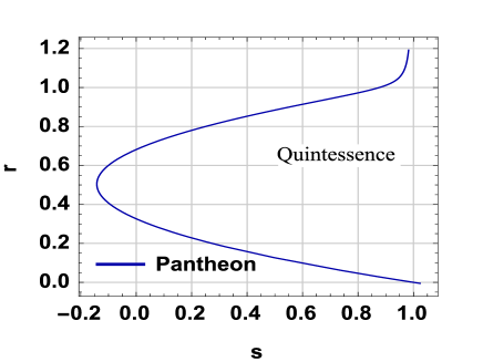
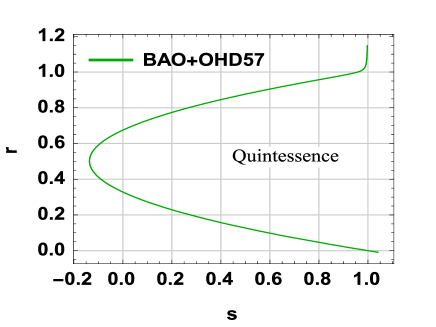
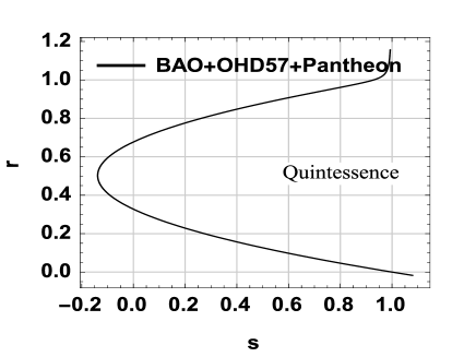
For various best-fitted values of free parameters for the different observational datasets, the trajectories depicting the evolutionary behavior of the model in plane are shown in Figure 6. The figure shows that the model lies in the quintessence region . By using these Statefinder parameters, researchers can probe the dynamics of the universe and differentiate between different dark energy models more effectively [61, 67, 68].
9 Speed of sound
The sound speed should be necessarily less than the speed of light (). The velocity of sound exists within the range with cosmic time, as we are working with gravitational units with a unit speed of light time [73, 74, 75]. The formula for the square of sound speed is:
| (35) |
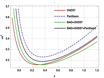
To ensure the stability of the given theoretical model, the velocity () should lie within the range of -1 to 1 for the redshift scale. By examining Figure 7, we can see that the sound speed consistently lies within this specified range throughout the evolution of the universe.
10 Classical linear and nonlinear Energy Conditions
In the context of general relativity, energy conditions are used to explore the properties and behaviors of space-time, and they play a role in various theorems and conjectures related to the nature of gravity and the possibility of constructing "exotic" configurations of matter that might lead to violations of certain physical principles. There are several energy conditions, and they fall into two main categories: linear energy conditions and non-linear energy conditions. In classical physics, energy conditions are linear, meaning that they have straightforward requirements on the stress-energy tensor that ensure the conservation of energy and other fundamental physical properties. However, in certain cases, nonlinear energy conditions are considered to explore more exotic scenarios that could potentially violate some of the standard assumptions. These conditions are used in the study of general relativity and are closely related to the concept of exotic matter and the possibilities of faster-than-light travel and traversable wormholes.
The linear energy conditions (ECs) within the framework of GR are mathematically explained as (1) Weak Energy Condition (WEC): , , (2) Null Energy Condition (NEC): , (3) Dominant Energy Condition (DEC): , (4) Strong Energy Condition (SEC): [76, 77].
In addition, non linear energy conditions are :
1. The flux EC:
2. The determinant EC:
3. The trace of square EC:
(a)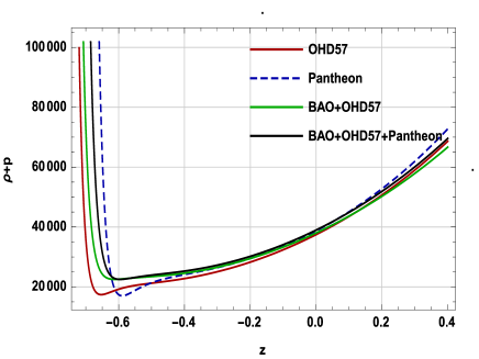 (b)
(b)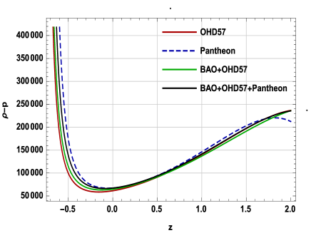 (c)
(c)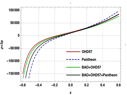 (d)
(d)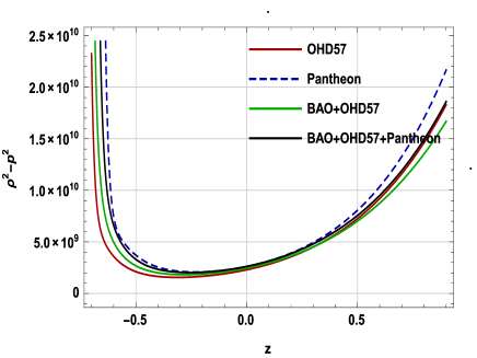 (e)
(e)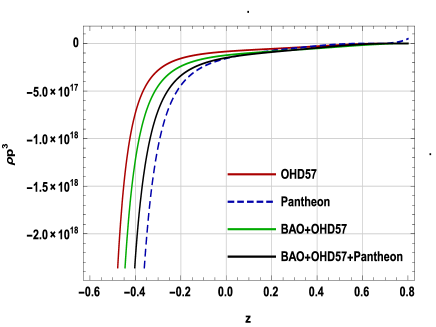 (f)
(f)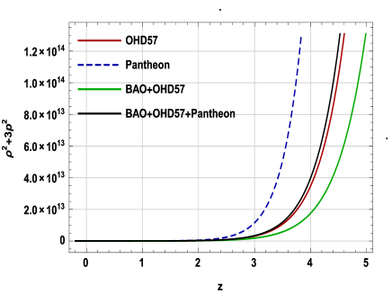
Figure 8 illustrates the accomplishment of energy conditions for the proposed model using the joint observational data from BAO, OHD, and Pantheon. The derived model satisfies WEC, DEC, and NEC, but violates SEC as depicted in Figure 8. The violation of SEC for the proposed model depicts the accelerated expansion of the cosmos and confirms the presence of exotic matter in the cosmos [76, 77, 78]. The term "flux" generally refers to the flow of some physical quantity through a surface. The tensor of stress energy is efficient in describing the flow of energy, momentum, or stress across a particular area. In the case of the Null Energy Condition, the NEC requires that the flux of the stress-energy tensor’s components should be non-negative for all null (light-like) vectors. This helps to ensure that the energy density along any null geodesic remains non-negative.
The ‘trace’ of the ‘stress-energy tensor’ is the sum of its diagonal components, that typically correspond to pressure and energy density. In the context of the Strong Energy Condition, the trace condition often states that the summation of three times the pressure and the energy density should be non-negative. Figures 8(d), 8(e), 8(f) show the non-linear energy conditions. The Flux and the trace of the square of both ECs are satisfied. Non-linear energy conditions are particularly important in investigations of exotic matter and space-time geometries that might allow for phenomena like faster-than-light travel, time travel, or other violations of classical energy conditions. They help to identify regions of space-time where such exotic behavior might occur or be ruled out.
11 Concluding remarks
This article focuses on examining a modified theory known as the Weyl gravity, where the relationship between metric and the Weyl vector plays an important role in determining the metric tensor’s covariant divergence. Consequently, the geometrical properties of the theory are impacted by both the metric tensor and the Weyl vector. We have explored the universe’s dynamics utilizing the parametric form of DP represented as . To estimate the free parameters , , and , we have utilized the latest experimental datasets of BAO, OHD, and Pantheon and implementing the application of the MCMC method. We have employed the open-source Python package ‘emcee’ for this purpose. Additionally, we have determined a few kinetic properties such as , quintessence, state-finders, sound speed, and energy conditions which provide further insights into the behavior and implications within this context. The highlights of the model are given below.
-
•
We have used three distinct sets of observational data: Baryon Acoustic oscillation(BAO), Observational Hubble Data (OHD), and data from Pantheon compilation. Implementing the MCMC statistical approach, we have estimated the free parameters , , and . Taking the joint dataset into account, the confidence contour for model parameters is plotted in Figure 1. The constrained values of model parameters are tabulated in Table 1.
-
•
The evolutionary behaviours of the energy density and cosmic pressure are represented in Figures 2(a) and 2(b) respectively. For all observational datasets, the nature of the energy density is positive while nature of cosmic pressure is negative throughout the evolution.
-
•
Figure 3 shows the EoS parameter for the three models of Weyl type gravity. It has been plotted for the observational values. During its evolution, the derived model initially lies in quintessence era and advanced to Chaplygin gas scenario in late time.
-
•
In Figure 4, we have described the for all the observational values. It is found that the curve lies in both thawing and freezing regions.
-
•
The nature of scalar potential and scalar field for Weyl type of gravity is depicted in Figure 5. We observe that the potential for the quintessence model is a decreasing function of , which gives rise to an accelerated expansion. The behavior of the state-finders is shown in Figure 6. The trajectories for the proposed models lie in quintessence region as shown in the figure. For the proposed model, the sound speed’s nature can provide insights into its stability and characteristics. The trajectories of sound speed for different observational data sets are plotted in Figure 7.
-
•
Figure 8 shows linear and nonlinear energy conditions of the proposed model for observational datasets. The violation of SEC for the derived model depicts an accelerated expansion of the cosmos. Figures 8(d), 8(e), 8(f) show the non-linear energy conditions. The Flux and trace of square both ECs are satisfied.
In the manuscript, we have present a comprehensive study of an accelerated expanding cosmological model in Weyl gravity with the aid of a specific parametric approach.
References
- [1] A.G. Riess, et al., Observational evidence from supernovae for an accelerating universe and a cosmological constant, Astron. J. 116 (1998) 1009.
- [2] S. Perlmutter, et al., Measurements of and from 42 high-redshift supernovae, Astrophys. J. 517 (1999) 565.
- [3] R.R. Caldwell, M. Doran, Cosmic microwave background and supernova constraints on quintessence: concordance regions and target models, Phys. Rev. D 69 (2004) 103517.
- [4] D.N. Spergel et al., First-Year Wilkinson Microwave Anisotropy Probe Observations: Determination of Cosmological Parameters, Astrophys. J. Suppl. 148, 175 (2003)
- [5] E. Komatsu et al., Five-year wilkinson microwave anisotropy probe (WMAP) observations: cosmological interpretation, Astrophys. J. Suppl. 180 (2009) 330.
- [6] A.G. Riess et al., Type Ia supernova discoveries at from the Hubble space telescope: Evidence for past deceleration and constraints on dark energy evolution, Astrophys. J. 607 (2004) 665.
- [7] T. Koivisto, D.F. Mota, Dark energy anisotropic stress and large scale structure formation, Phys. Rev. D 73 (2006) 083502.
- [8] S. Nojiri and S.D. Odintsov, Unifying phantom inflation with late-time acceleration: scalar phantom-non-phantom transition model and generalized holographic dark energy, Gen. Relativ. Gravit. 38 (2006) 1285.
- [9] J. Matsumoto and S. Nojiri, Reconstruction of k-essence model, Phys. Lett. B 687, 236 (2010).
- [10] B.P. Schmidt, et al., The high-Z supernova search: Measuring cosmic deceleration and global curvature of the universe using yype Ia supernovae, Astrophys. J. 507 (1998) 46.
- [11] S. Perlmutter, et al., Discovery of a supernova explosion at half the age of the universe and its cosmological implications, Nature 391 (1998) 51.
- [12] G. R. Bengochea and R. Ferraro, Dark torsion as the cosmic speed-up, Phys. Rev. D 79 (2009) 124019.
- [13] R. Myrzakulov, gravity and k-essence, Gen. Rel. Grav. 44, (2012) 3059.
- [14] S. Nojiri and S. D. Odintsov, Modified Gauss–Bonnet theory as gravitational alternative for dark energy, Phys. Lett. B 631 (2005) 1.
- [15] A. De Felice and S. Tsujikawa, Construction of cosmologically viable gravity models, Phys. Lett. B 675 (2009) 1.
- [16] G. Cognola, E. Elizalde, S. Nojiri, S. D. Odintsov and S. Zerbini, Dark energy in modified Gauss-Bonnet gravity: Late-time acceleration and the hierarchy problem, Phys. Rev. D 73 (2006) 084007.
- [17] I. H. Brevik and J. Quiroga Hurtado, Vanishing Cosmological Constant in Modified Gauss-Bonnet Gravity with Conformal Anomaly, Int. J. Mod. Phys. D 16 (2007) 817.
- [18] E. Elizalde, A. N. Makarenko, V. V. Obukhov, K. E. Osetrin and A. E. Filippov, Stationary vs. singular points in an accelerating FRW cosmology derived from six-dimensional Einstein–Gauss–Bonnet gravity, Phys. Lett. B 644 (2007) 1.
- [19] K. Bamba, S. D. Odintsov, L. Sebastiani and S. Zerbini, Finite-time future singularities in modified Gauss–Bonnet and gravity and singularity avoidance, Eur. Phys. J. C 67 (2010) 295.
- [20] S. Bahamonde, M. Zubair and G. Abbas, Thermodynamics and cosmological reconstruction in gravity, Phys. Dark Univ. 19 (2018) 78.
- [21] T. P. Sotiriou and V. Faraoni, theories of gravity, Rev. Mod. Phys. 82 (2010) 451.
- [22] S. Capozziello, Curvature quintessence, Int. J. Mod. Phys. D 11 (2002) 483.
- [23] S. M. Carroll, V. Duvvuri, M. Trodden and M. S. Turner, Is cosmic speed-up due to new gravitational physics?, Phys. Rev. D 70 (2004) 043528 .
- [24] S. Capozziello, V. F. Cardone and A. Troisi, Dark energy and dark matter as curvature effects?, JCAP 08, 001 (2006).
- [25] C. G. Boehmer, T. Harko and F. S. N. Lobo, Dark matter as a geometric effect in gravity, Astropart. Phys. 29 (2008) 386.
- [26] T. Chiba, 1/R gravity and scalar-tensor gravity, Phys. Lett. B 575 (2003) 1.
- [27] A. L. Erickcek, T. L. Smith and M. Kamionkowski, Solar system tests do rule out gravity, Phys. Rev. D 74 (2006) 121501.
- [28] R. Myrzakulov, FRW cosmology in gravity, Eur. Phys. J. C 72 (2012) 2203.
- [29] T. Harko, F.S.N. Lobo, S. Nojiri, S.D. Odintsov, gravity, Phys.Rev. D 84 (2011) 024020.
- [30] A. K. Yadav, L. K. Sharma, B. K. Singh, and P. K. Sahoo, Existence of bulk viscous universe in gravity and confrontation with observational data, New Astron. 78 (2020) 101382.
- [31] V.K. Bhardwaj, A.K. Yadav, Some Bianchi type-V accelerating cosmological models in formalism, Int. J. Geom. Methods Mod. Phys. 17 (2020) 2050159.
- [32] L.K. Sharma, A.K. Yadav, and B.K. Singh, Power-law solution for homogeneous and isotropic universe in gravity, New Astronomy 79 (2020) 101396.
- [33] A. Pradhan, G.K. Goswami, and A. Beesham, The reconstruction of constant jerk parameter with gravity, Journal of High Energy Astrophysics 38 (2023) 12-21.
- [34] S. Capozziello et al., Phys. Rev. D, 84, 043527 (2011).
- [35] Di Liu, M. J. Reboucas, Phys. Rev. D, 86, 083515 (2012).
- [36] Deng Wang, David Mota, Phys. Rev. D, 102, 063530 (2020).
- [37] S. Bhattacharjee and P. K. Sahoo, Eur. Phys. J. C 80, 289 (2020).
- [38] S. Arora et al., Phys. Dark Univ. 30, 100664 (2020).
- [39] R. Zia, D. C. Maurya and A. K. Shukla, Int. J. Geom. Methods Mod. Phys. 18, 2150051 (2021).
- [40] T.H. Loo et al., Eur. Phys. J. C 83 (2023) 261.
- [41] Y. Xu et al., Eur. Phys. J. C 80, 449 (2020).
- [42] Jin-Z. Yang et al., Eur. Phys. J. C 81, 111 (2021).
- [43] G. Gadbail, S. Arora, and P.K. Sahoo, Eur. Phys. J. Plus 136, 1040 (2021).
- [44] G. Gadbail, S. Arora, and P.K. Sahoo, Eur. Phys. J. C 81, 1088 (2021).
- [45] G. N. Gadbail, S. Arora, P. Kumar, and P. K. Sahoo, Chin. J. Phys. 79, 246-255 (2022).
- [46] J.B. Jimenez, L. Heisenberg, T.Koivisto, Phys. Rev. D, 98, 044048 (2018)
- [47] L. Xu, H. Liu, Constraints to deceleration parameters by recent cosmic observations, Mod. Phys. Lett. A 23 (2008) 1939.
- [48] G. S. Sharov, V. O. Vasiliev, Math. Model. Geom. 6 (2018) 1.
- [49] H. Yu et al., Hubble parameter and Baryon Acoustic Oscillation measurement constraints on the Hubble constant, the deviation from the spatially flat CDM model, Astrophys. J. 856 (2018) 3.
- [50] D. M. Scolnic et al., The complete light-curve sample of spectroscopically confirmed SNe Ia from Pan-STARRS1 and cosmological constraints from the combined pantheon, Astrophys. J. 859 (2018) 101.
- [51] F. Beutler et al., The 6dF Galaxy Survey: baryon acoustic oscillations and the local Hubble constant, Mon. Notices Royal Astron. Soc. 416 (2011) 3017 .
- [52] L. Anderson et al., The clustering of galaxies in the SDSS-III Baryon Oscillation Spectroscopic Survey: baryon acoustic oscillations in the Data Releases 10 and 11 Galaxy samples, Mon. Notices Royal Astron. Soc. 441 (2014) 24.
- [53] N. Padmanabhan et al., A 2 per cent distance to z = 0.35 by reconstructing baryon acoustic oscillations – I. Methods and application to the Sloan Digital Sky Survey, Mon. Notices Royal Astron. Soc. 427 (2012) 2132.
- [54] C. Blake et al., The WiggleZ Dark Energy Survey: joint measurements of the expansion and growth history at , Mon. Notices Royal Astron. Soc. 425 (2012) 405.
- [55] M. Koussour, et al., Dynamical dark energy models from a new Hubble parameter in gravity, arXiv preprint arXiv:2208.04723 (2022).
- [56] O. Farooq, B. Ratra, Astrophys. J. Lett. 766 (2013) L7.
- [57] E.O. Colgain, M. M. Sheikh-Jabbari, Euro. Phys. J. C 81 (2021) 892.
- [58] Luongo, O., et al., Phys. Rev. D 105 (2022) 103510.
- [59] V.K. Bhardwaj et al., Corrected holographic dark energy with power-law entropy and Hubble Horizon cut-off in FRW Universe, Chinese Journal of Physics 79 (2022) 471-480.
- [60] M.V.D. Santos et al., J. Cosmo. Astro. Phys. 2016 (2016) 066.
- [61] P. Shrivastava et al., Galaxies 11 (2023) 57.
- [62] Bum-Hoon Lee et al., J. Cosmo. Astropart. Phys. 2022.04 (2022) 004.
- [63] R. R. Caldwell, E.V. Linder, Limits of Quintessence, Phys. Rev. Lett. 95 (2005) 141301.
- [64] T. Chiba, and of scalar field models of dark energy, Phys. Rev. D 73 (2006) 063501.
- [65] Z. K. Guo et al., Two-field quintom models in the plane, Phys Rev D 74 (2006) 127304.
- [66] M. Malekjani, A.K. Mohammadi, Statefinder diagnostic and analysis for interacting polytropic gas dark energy model, Int J Theor Phys 51 (2012) 3141.
- [67] S. Tsujikawa, Quintessence: A review, Class. Quant. Grav. 30 (2013) 214003.
- [68] V.K. Bhardwaj, Observation constraints on scalar field cosmological model in Anisotropic universe, arXiv preprint arXiv:2308.02864 (2023).
- [69] A. Ali, R. Gannouji, M. Sami, A.A. Sen, Background cosmological dynamics in gravity and observational constraints, Phys. Rev. D 81 ( 2010) 104029.
- [70] M. Malekjani, A. Khodam-Mohammadi, Statefinder diagnosis and the interacting ghost model of dark energy, Astrophys. Space Sci. 343 (2013) 451.
- [71] U. Alam, V. Sahni, T.D. Saini, A.A. Starobinsky, Exploring the expanding universe and dark energy using the Statefinder diagnostic, Mon. Not. Roy. Astron. Soc. 344 (2003) 1057.
- [72] V.K. Bhardwaj, Current Observation constraints on Hybrid potential scalar field cosmological model in Lyra Geometry." arXiv preprint arXiv:2309.10282 (2023).
- [73] G.B. Zhao, et al., Perturbations of the quintom models of dark energy and the effects on observations, Phys. Rev. D 72 (2005) 123515.
- [74] V. Sahnia, A. Shafielooa, and A.A. Starobinsky, Two new diagnostics of dark energy,Physical Review D 78.10 (2008) 103502.
- [75] P.A.R. Ade et. al., Plank 2015 Results cosmological parameters, Astron. Astrophys. 594 (2016) A13.
- [76] S. Capozziello, S. Nojiri, S.D. Odintsov, The role of energy conditions in cosmology, Phys. Lett. B 781, 99-106 (2018).
- [77] S. E. Perez Bergliaffa, Constraining theories with the energy conditions, Phys. Lett. B 642, 311-314 (2006).
- [78] V.K. Bhardwaj, P. Garg, New Astronomy 105 (2024) 102101.