Hierarchical Adaptation with Hypernetworks for Few-shot Molecular Property Prediction

Abstract

Molecular property prediction (MPP) is important in biomedical applications, which naturally suffers from a lack of labels, thus forming a few-shot learning problem. State-of-the-art approaches are usually based on gradient-based meta learning strategy, which ignore difference in model parameter and molecule’s learning difficulty. To address above problems, we propose a novel hierarchical adaptation mechanism for few-shot MPP (HiMPP). The model follows a encoder-predictor framework. First, to make molecular representation property-adaptive, we selectively adapt encoder’s parameter by designing a hypernetwork to modulate node embeddings during message propagation. Next, we make molecule-level adaptation by design another hypernetwork, which assigns larger propagating steps for harder molecules in predictor. In this way, molecular representation is transformed by HiMPP hierarchically from property-level to molecular level. Extensive results show that HiMPP obtains the state-of-the-art performance in few-shot MPP problems, and our proposed hierarchical adaptation mechanism is rational and effective.

1 Introduction

Molecular property prediction (MPP) (Wieder et al., 2020) which predicts whether desired properties will be active on given molecules, can be naturally modeled as a few-shot learning problem (Waring et al., 2015; Altae-Tran et al., 2017). As the wet-lab experiments to evaluate the actual properties of molecules are expensive and risky, usually only few labeled molecules are available for certain property. While recently, large Graph Neural Networks (GNN) are popularly used to learn representations for molecules (Xu et al., 2019; Yang et al., 2019; Xiong et al., 2019). Modeling molecules as graphs, GNN can capture inherent structural information from the level of composition of atoms and chemical bonds. Hence, GNN-based MPP methods have shown significant better performance than classical ones (Unterthiner et al., 2014; Ma et al., 2015), especially when they are pretrained on self-learning tasks. As for tasks with only few labeled molecules, performance of existing GNN-based methods are still far from desired.

Existing works adopt gradient-based meta learning strategy to handle the few-shot MPP problem. They mainly design their approaches based on Model-Agnostic Meta-Learning (MAML) (Finn et al., 2017), which learns parameter initialization with good generalizability across different properties and adapts parameters by gradient descent for the test property. Specifically, Meta-MGNN (Guo et al., 2021) brings chemical prior knowledge in the form of molecular reconstruction loss. PAR (Wang et al., 2021) introduces attention and relation graph module to better utilize the labeled samples for property-adaptation with the awareness of target chemical property. However, this gradient-based meta learning strategy still can not avoid updating a large number of parameters with few shot to adapt to each task. This results in poor learning efficiency and prone to over-fit with insufficient labeled samples (Rajeswaran et al., 2019; Yin et al., 2020). Instead, the model parameters should be selectively adapted. Another problem in these works is ignoring molecule-level difference. For MPP, we notice that molecule-level difference should be addressed when classifying the encoded molecules since chemical space is enormous that the representations of molecules vary in a wide range even in the same task. There are molecules which are much more similar with labeled molecules in one certain class, which can be easily classified. While others are difficult as they bear close similarities with the two given classes. Existing works ignore this, and a fixed predictor can not fit all molecules in a task. Thus, to make accurate MPP, not only property-level adaptation should be made according to the target property of the task, molecule-level adaptation should also be addressed to take molecule-level difference into consideration.

To address the above-mentioned two problems, we propose HiMPP, a few-shot MPP model with hierarchical adaptation mechanism by hypernetworks. Hypernetworks (Ha et al., 2017) are neural networks that generate parameters for main network. With domain knowledge to handcraft problem-specifically, hypernetworks can make adaptation on the main network according to the input information. To selectively adapt parameters, we design a hypernetwork to map the labeled graphs to task-specific parameter which is only a small amount, to modulate the GNN for property-adaptive representation, achieving the property-level adaptation. To capture the molecule-level difference, inspired by curriculum learning (Bengio et al., 2009) which considers sample-level difference by assigning certain learning order for samples with different difficulties, we propose a novel molecule-level adaptation that assigns more complex models for molecules that are difficult to classify. We build another hypernetwork which functions as a controller of a dynamic propagation on a relation graph-based predictor, where the propagation steps is different for molecules with different predicting difficulty, achieving molecule-level adaptation. Our contributions are summarized as follows:

• We propose a hierarchical adaptive mechanism for few-shot MPP to first adapt on property-level effectively by selectively adapting parameters, and further achieve molecule-level adaptation by dynamic propagation.

• We design two hypernetworks for property-level and molecule-level adaptation respectively, which work sequentially in a encoder-predictor MPP model. The hypernetwork for encoder maps a set of labeled graphs to property-specific parameters to modulate GNN. The hypernetwork for predictor explicitly encode the model architecture to control a dynamic propagation.

• Extensive results show HiMPP obtains the state-of-the-art performance in few-shot MPP problems. We also show the rationality and effectiveness of the hierarchical adaptation mechanism.

2 Related Works

2.1 Molecular Property Prediction (MPP)

In conventional cheminformatics, molecules are described with certain properties (fingerprint vectors (Rogers and Hahn, 2010)) and fed to feed-forward networks (Unterthiner et al., 2014; Ma et al., 2015). Recently, as GNNs have shown superior performance on learning from of topological data, and the nature to represent a molecule as a graph where atoms are viewed as vertices and the chemical bonds as edges, GNNs are popularly taken as molecular encoders (Li et al., 2018; Yang et al., 2019; Xiong et al., 2019; Hu et al., 2019). Given molecular graph as input features, MPP models are built under an encoder-predictor framework. A GNN-based encoder is used to map molecular graphs to molecular representations which are vectors with fixed length. Then, the predictor classifies the representations.

Since GNNs require training from a large amount of labeled data, it is widely focused on that pre-training GNN encoders in a self-supervised manner on large datasets (Hu et al., 2019; Xu et al., 2021; Zhang et al., 2021; Hou et al., 2022), then transfer the pre-trained GNN encoders to downstream. The learning on self-supervised tasks, e.g., masking and predicting atoms and chemical bonds, or incorporating 3D information and matching representation pairs encoded from 2D/3D information of the same molecule (Liu et al., 2022; Stärk et al., 2022), can equip the GNN encoder with generalizable knowledge to capture structural information and represent molecular graphs. However, adopting a pre-trained GNN encoder for downstream MPP tasks still requires task-adaptation and may suffer over-fitting the few-shot. Meta-MGNN (Guo et al., 2021) adapts its encoder this by MAML, and PAR (Wang et al., 2021) introduces property-aware attention.

While the encoder can generalize to different tasks as capturing structural information from the composition of atoms, the predictor needs property-level adaptation on downstream task. IterRefLSTM (Altae-Tran et al., 2017) builds a matching network in predictor which is property-adaptive where all molecular representations are effected by a recurrent neural network taking the labeled samples as input, and classify by pair-wise similarity. and Meta-MGNN incorporates a multi-layer perceptron (MLP) classifier as predictor and all parameters is property-adaptive via adopting MAML. For the predictor in PAR, a relation graph is built between samples to refine the representations. It also adopts MAML to train that the whole model is property-adaptive.

2.2 Hypernetworks

Hypernetworks (Ha et al., 2017) refer to neural networks which are learned to generate parameters for another neural network. The main network learns to map some raw inputs to their desired targets, whereas another group of inputs are fed to the hypernetwork to generate parameters to adapt the main network. It has been successfully used to handle various applications like neural architecture search (Brock et al., 2018), multi-agent reinforcement learning (Rashid et al., 2018), neural non-linearity design  (Sitzmann et al., 2020) and few-shot learning (Requeima et al., 2019). Specially in few-shot learning, hypernetworks aggregate support data and generate task-specific parameter for main network (Przewiezlikowski et al., 2022).

The design of hypernetworks is challenging and highly-specific to the problem. It requires domain knowledge to design what information should be fed to the hypernetwork that the main network would be adapted to, and how to design neural structure to learn effectively, and what components of the main network should be adapted, and by what function. For example, for task-adaptation on CNN model (Requeima et al., 2019), it has been used to map images to adaptive parameters of feature-wise linear modulation (FiLM) layers (Perez et al., 2018) in convolution blocks. For node-adaptive message passing function in GNN model, Brockschmidt (2020) builds hypernetworks with target node as input to generate parameters to modulate weight matrix in aggregation function in message passing. And Nachmani and Wolf (2020) study that hypernetwork for node-specific message passing functions can lead to a boost in performance. Note that though above two works introduce hypernetworks into GNN and MPP, the purpose and usage are completely different with ours. Their hypernetworks are designed for more powerful GNN model while ours are designed to achieve hierarchical adaptation, which means their model can be incorporated in our method as molecular encoder.

3 Proposed Method

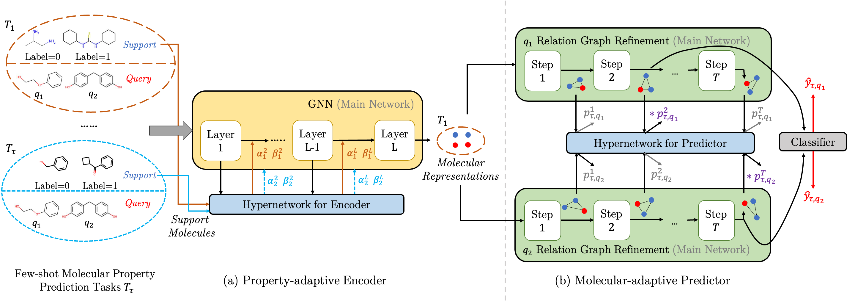
Figure 1: Illustration of the proposed HiMPP. In the encoder, property-level adaptation is achieved by modulating node embeddings during message passing via FiLM layers. In the predictor, molecule-level adaptation is achieved by dynamic propagation with molecule-specific steps.

3.1 Problem Setup and Architecture Overview

Following the definition of few-shot MPP adopted by earlier works (Altae-Tran et al., 2017; Guo et al., 2021; Wang et al., 2021), we view it as a $2$-way $K$-shot classification task $\mathcal{T}_{\tau}$, where a support set $\mathcal{S}_{\tau}=\{(\mathcal{X}_{{\tau},i},y_{{\tau},i})\}_{i=1}^{2\times K}$ contains $K$ samples from each class and a query set $\mathcal{Q}_{\tau}=\{({\mathcal{X}}_{{\tau},j},{y}_{{\tau},j})\}_{j=1}^{M}$ contains $M$ samples whose labels are only used to test the classification model. The aim is to learn a model from a set of tasks $\{\mathcal{T}_{\tau}\}_{j=1}^{N_{t}}$ that can generalize to new task given the support set. In the context of MPP, each task $\mathcal{T}_{\tau}$ is to learn to predict certain target property using given few labeled molecule. Specifically, each sample $\mathcal{X}_{{\tau},i}$ is a molecular graph and $y_{{\tau},i}\in\{0,1\}$ records whether the molecule is inactive or active on the target property. The target properties are different across tasks.

The architecture of the proposed HiMPP is illustrated as Figure 1, where the main network is built under the encoder-predictor framework. To achieve the hierarchical adaptation, we introduce two hypernetworks into the encoder for property-level and predictor for molecule-level adaptation respectively.

3.2 Design of the Main Network

The main network of HiMPP follows the encoder-predictor framework to make prediction for molecular graphs. A GNN-based encoder is used to map molecular graphs to molecular representations which are vectors with fixed length. Then, the predictor classifies the representations.

Consider a molecular graph $\mathcal{X}=\{\mathcal{V},\mathcal{E}\}$ with node feature $\mathbf{h}_{v}$ for each atom $v\in\mathcal{V}$ and edge feature $\mathbf{b}_{vu}$ for each chemical bond $e_{vu}\in\mathcal{E}$ between atoms $v,u$. At the $l$th layer, GNN updates the atom embedding $\mathbf{h}_{v}^{l}$ using message $\mathbf{h}_{\text{agg}}^{l-1}$:

$$\mathbf{h}_{\text{agg}}^{l-1} =\texttt{AGG}^{l}\left(\{(\mathbf{h}_{v}^{l-1},\mathbf{h}_{u}^{l-1},\mathbf{b}_{vu})|u\in\mathcal{H}(v)\}\right),$$ (1)

$$\mathbf{h}_{v}^{l} =\texttt{UPDATE}^{l}\left(\mathbf{h}_{v}^{l-1},\mathbf{h}_{\text{agg}}^{l-1}\right),$$ (2)

where $\mathcal{H}(v)$ is a set of chemically bonded neighbor atoms of $v$. After $L$ iterations, the molecule-level representation $\mathbf{r}$ for $\mathcal{X}$ is obtained as

$$\mathbf{r}=\texttt{READOUT}\left(\{\mathbf{h}_{v}^{L}|v\in\mathcal{V}\}\right),$$ (3)

where $\texttt{READOUT}(\cdot)$ function aggregates all atom embeddings into the molecular representation. Specifically, we adopt a GIN (Xu et al., 2019) which specifies AGG, UPDATE and READOUT, as it is a powerful and popularly used GNN model.

The encoder gets molecular representation $\mathbf{r}_{\tau,i}$ for each molecule $\mathcal{X}_{{\tau},i}$, which are then fed to the predictor. Relation graph (Garcia and Bruna, 2018; Wang et al., 2021) is an effective predictor model for few-shot learning, which can refine molecular representations such that the similar molecules cluster closer. To construct relation graphs, the output of the encoder is taken as the initial molecular representations, i.e., $\mathbf{r}_{\tau,i}^{0}=\mathbf{r}_{\tau,i}$. Denote the query index as $q$, i.e., $\mathcal{Q}_{\tau}$ $=$ $\{({\mathcal{X}}_{{\tau},q},$ ${y}_{{\tau},q})\}_{q=1}^{M}$, and $\mathcal{R}_{{\tau},q}=({\mathcal{X}}_{{\tau},q},{y}_{{\tau},q})\cup\mathcal{S}_{\tau}$. The relation graph works as recurrently estimating the adjacency matrix and updating the molecular representations. Its adjacent matrix which represents pair-wise similarities between molecules in $\mathcal{R}_{{\tau},q}$, is denoted as $\mathbf{A}_{{\tau},q}^{t}$ at the $t$th step . We first construct $\mathbf{A}_{{\tau},q}^{t}$ as

$$\left[\mathbf{A}_{\tau,q}^{t}\right]_{ij}=\begin{cases}\texttt{MLP}_{A}\left(\text{exp}(|\mathbf{r}_{{\tau},i}^{t-1}-\mathbf{r}_{{\tau},j}^{t-1}|)\right)&\text{if\;}i\neq j\\ 1&\text{otherwise}\end{cases}.$$

Next, all molecular representations are refined by

$${\bm{R}}_{\tau}^{t}=\texttt{MLP}_{N}(\mathbf{A}_{\tau}^{t}{\bm{R}}_{{\tau},q}^{{t}-1}),$$ (4)

where ${\bm{R}}_{{\tau},q}^{t}$ is the collection of $\mathbf{r}_{\tau,i}^{t}$, the representation vectors refined by $t$ steps of all molecules contained in $\mathcal{R}_{{\tau},q}$. After several steps of refinement, a classifier will generate the final prediction $\hat{\bm{y}}_{{\tau},q}^{t}$ for the query $\mathbf{r}_{{\tau},q}^{{t}}$, according to the other $2K$ labeled support samples $\{(\mathbf{r}_{{\tau},i}^{{t}},y_{{\tau},i})~{}|~{}\mathcal{X}_{{\tau},i}\in\mathcal{S}_{\tau}\}$.

Above model with encoder-predictor framework can learn to map molecular graphs to labels to predict certain property. Existing works (Guo et al., 2021; Wang et al., 2021) adopt MAML for property-level adaptation. While MAML can also be incorporated in above framework (see Appendix A.3), we design hypernetworks to bring the advantage to selectively adapt parameter on property-level and ability to adapt on molecule-level.

3.3 Design of the Hypernetworks

As mentioned in Section 1, both property-level (task-level) and molecule-level adaptation are important for prediction a molecule. The property-level adaptation is addressed in encoder such that each molecule can have property-adaptive representation according to the task. Molecule-level adaptation is considered for difference of classification complexity between molecules, thus is incorporated in predictor. We design hypernetwork for encoder and hypernetwork for predictor respectively.

3.3.1 Hypernetwork for Encoder

As tasks target on different properties, the property-level adaptation aims to capture information from $\mathcal{S}_{\tau}$ to make better prediction for $\mathcal{Q}_{\tau}$. The main network in encoder is GNN to capture shared structural patterns of molecular graphs, like functional groups which are generalizable across tasks. However, features in embedding play different roles in contribution to different properties. Labeled molecules in each property contains its own specific information like which dimension of feature is more decisive. Thus, a hypernetwork can work to modulate node embedding $\mathbf{h}_{v}$ based on property specific information in $\mathcal{S}_{\tau}$ during the propagation.

As for how to adapt, it should be parameter-friendly while effective to address the selective adaptation. Inspired by Brockschmidt (2020), we choose to use a feature-wise linear modulation (FiLM) (Perez et al., 2018) layer after every layer of the GNN, as it is simple and effective in GNN. At the $l$th layer, to obtain the adaptive embedding $\hat{\mathbf{h}}_{v}^{l-1}$ for each atom $v\in\mathcal{X}_{{\tau},i}$,

$$\hat{\mathbf{h}}_{v}^{l-1}=\bm{\alpha}_{\tau}^{l}\odot\mathbf{h}_{v}+\bm{\beta}_{\tau}^{l},$$ (5)

where $\odot$ means element-wise product, and $[\bm{\alpha}_{\tau}^{l},\bm{\beta}_{\tau}^{l}]$ is property-specific parameter generated by the hypernetwork to parameterize a FiLM function. Then we follow the message passing (1) (resp. (2)) where we use the modulated $\hat{\mathbf{h}}_{u}^{l-1}$ instead of $\mathbf{h}_{u}^{l-1}$ (resp. $\hat{\mathbf{h}}_{v}^{l-1}$ instead of $\mathbf{h}_{v}^{l-1}$). After $L$ layers of message passing and modulation, the property-adaptive molecular representation $\hat{\mathbf{r}}_{\tau,i}$ can be obtained by (3).

The last question is how to generate $\bm{\alpha}_{\tau}^{l}$ and $\bm{\beta}_{\tau}^{l}$, which should contain property-specific information learned from $\mathcal{S}_{\tau}$. As $\mathcal{S}_{\tau}$ is a set, the hypernetwork for encoder need to be permutation-invariant for $\mathcal{X}_{{\tau},i}\in\mathcal{S}_{\tau}$. Let $\bm{r}_{{\tau},+}^{l}$ (resp. $\bm{r}_{{\tau},-}^{l}$) be the average representation at the $l$th GNN layer for positive (negative) samples in task ${\tau}$, which is computed as

$$\bm{r}_{{\tau},\pm}^{l}=\frac{1}{|\mathcal{S}_{\tau}^{\pm}||\mathcal{V}_{{\tau},i}|}\sum\nolimits_{\mathcal{X}_{{\tau},i}\in\mathcal{S}_{\tau}^{\pm}}\sum\nolimits_{v\in\mathcal{X}_{{\tau},i}}\big{[}\mathbf{h}_{v}^{l}~{}|~{}\bm{y}_{{\tau},i}\big{]},$$ (6)

where $\mathcal{S}_{\tau}^{\pm}$ is the set of positive (resp. negative) molecules in $\mathcal{S}_{\tau}$ and $\bm{y}_{{\tau},i}$ is the one-hot encoding of label. Then, the hypernetwork is constructed as

$$\left[\bm{\alpha}_{\tau}^{l},\bm{\beta}_{\tau}^{l}\right]=\texttt{MLP}^{l}_{E}\left(\left[\bm{r}_{{\tau},+}^{l}~{}|~{}\bm{r}_{{\tau},-}^{l}\right];\Theta_{E}^{l}\right),$$ (7)

where the MLP is parameterized by $\Theta_{E}^{l}$. As GNN encoder has $L$ layers, the hypernetwork for encoder needs $L$ MLPs in total.

3.3.2 Hypernetwork for Predictor

The relation graph in the predictor gathers information from all support molecules and update all representations to strengthen the similar and dissimilar between all supports and the query. However, there are query molecules that can be easily predicted with few refinement steps but also queries that bear close similarity with the two classes which are difficult to predict, for which more refinement steps can help. Thus, we achieve the molecule-level adaptation by dynamic propagation, that the number of steps $t$ should be specific to both support molecules in $\mathcal{S}_{\tau}$ and the query molecule in $\mathcal{Q}_{\tau}$, which could be controlled by our design of hypernetwork for predictor.

How to control $t$ is challenging since it is discrete to directly encode the refinement steps. Recall the notations in Section 3.2 and let $\mathcal{V}_{{\tau},q}^{t}=\mathbf{r}_{{\tau},q}^{{t}}\cup\{(\mathbf{r}_{{\tau},i}^{{t}},y_{{\tau},i})~{}|~{}\mathcal{X}_{{\tau},i}\in\mathcal{S}_{\tau}\}$. The hypernetwork returns a scalar $p_{{\tau},q}^{t}$ estimating how likely $\mathbf{r}_{{\tau},q}^{{t}}$ can be correctly classified given $\mathcal{V}_{{\tau},q}^{t}$. To calculate $p_{{\tau},q}^{t}$, similar to the hypernetwork for encoder, permutation-invariant inside $\{(\mathbf{r}_{{\tau},i}^{{t}},y_{{\tau},i})~{}|~{}\mathcal{X}_{{\tau},i}\in\mathcal{S}_{\tau}\}$ needs to be kept, so average each class and map all information in $\mathcal{V}_{{\tau},q}^{{t}}$ to a scalar:

$$p_{{\tau},q}^{t}=\texttt{MLP}_{P}\left(\left[\mathbf{r}_{{\tau},q}^{t}~{}|~{}\mathbf{r}_{{\tau},+}^{t}~{}|~{}\mathbf{r}_{{\tau},-}^{t}\right];\Theta_{P}\right),$$ (8)

and the parameter $\Theta_{P}$ is shared across all $t$. Finally, as there are $T$ steps in total, the vector

$$\bm{p}_{{\tau},q}=\texttt{softmax}([~{}p_{{\tau},q}^{1},~{}p_{{\tau},q}^{2},~{}\cdots,~{}p_{{\tau},q}^{T}~{}]),$$ (9)

represents the plausibility of choosing each time step. During meta-training, $\bm{p}_{{\tau},q}$ is used as differentiable weight so that gradients from classification loss can be propagated to parameter in the hypernetwork for predictor. The loss in a task $\mathcal{T}_{\tau}$ is calculated as

$$\mathcal{L}_{\tau}=-\sum\nolimits_{\bm{x}_{{\tau},q}\in\mathcal{Q}_{\tau}}\sum\nolimits_{{t}=1}^{T}[\bm{p}_{{\tau},q}]_{t}\cdot\bm{y}_{{\tau},q}^{\top}\text{log}\left(\hat{\bm{y}}_{{\tau},q}^{t}\right).$$ (10)

Comparing with conventional cross-entropy loss, minimizing the above objective encourages the hypernetwork for predictor to give layer with better classification performance a higher plausibility.

3.4 Learning and Inference

Denote the model parameter of the encoder and predictor in main network as $W_{E}$, $W_{P}$ respectively, then the collection of all model parameter is $\bm{\Theta}=\{\{\Theta_{E}^{l}\}_{l=1}^{L},\Theta_{P},W_{E},W_{P}\}$. Algorithm  1 summarizes the training procedure of HiMPP. In each episode, it learns each meta-training task one-by-one. For task $\mathcal{T}_{\tau}$, in the encoder, the hypernetwork for encoder and the GNN encoder in main network work iteratively for $L$ times to obtain property-adapted molecular representations (line 3-9). Then in the predictor, relation graphs are constructed for each query and updates for $T$ steps. At each step, a plausibility is generated by the hypernetwork for predictor and a classification loss is obtained (line 11-17). The plausibilities are used to weight the loss at different layers, and the summation of loss from all queries at each step is $\mathcal{L}_{\tau}$ (line 18). Finally, the gradient descent is used to optimize all parameters (line 19). Thus, in meta-training, all model parameters can be end-to-end optimized together via episodic training.

Algorithm 1 Meta-training in HiMPP.

0:  meta-training task set $\bm{\mathcal{T}}_{\text{train}}$

1:  initialize $\bm{\Theta}$ randomly;

2:  while not done do

3:     for each task $\mathcal{T}_{\tau}\in\bm{\mathcal{T}}_{\text{train}}$ do

4:        for $l\in\{1,2,\cdots,L\}$ do

5:           * calculate $\bm{\alpha}_{\tau}^{l}$ and $\bm{\beta}_{\tau}^{l}$ by (6) and (7);

6:           * modulate node embedding $\mathbf{h}_{v}^{l}$ by (5);

7:           + update node embedding $\mathbf{h}_{v}^{l}$ by (1)-(2);

8:        end for

9:     end for

10:     * obtain molecular representation $\hat{\mathbf{r}}_{\tau,i}$ by (3);

11:     for each query $({\mathcal{X}}_{{\tau},q},{y}_{{\tau},q})\in\mathcal{Q}_{\tau}$ do

12:        for $t\in\{1,2,\cdots,T\}$ do

13:           * update representations $\hat{\bm{R}}_{{\tau},q}^{t}$ by (4);

14:           + calculate $p_{{\tau},q}^{t}$ by (8);

15:        end for

16:        + calculate $\bm{p}_{{\tau},q}$ (9);

17:     end for

18:     obtain loss by (10);

19:     */+ update $\bm{\Theta}$ by gradient descent;

20:  end while

21:  return  learned $\bm{\Theta}^{*}$.

Algorithm 2 Meta-testing in HiMPP.

0:  learned $\bm{\Theta}*$, a meta-testing task $\mathcal{T}_{\tau}$;

1:  for $l\in\{1,2,\cdots,L\}$ do

2:     * calculate $\bm{\alpha}_{\tau}^{l}$ and $\bm{\beta}_{\tau}^{l}$ by (6) and (7);

3:     * modulate node embedding $\mathbf{h}_{v}^{l}$ by (5);

4:     + update node embedding $\mathbf{h}_{v}^{l}$ by (1)-(2);

5:  end for

6:  * obtain molecular representation $\hat{\mathbf{r}}_{\tau,i}$ by (3);

7:  for each query ${\mathcal{X}}_{{\tau},q}$ do

8:     for $t\in\{1,2,\cdots,T\}$ do

9:        * update representations $\hat{\bm{R}}_{{\tau},q}^{t}$ by (4);

10:        + calculate $p_{{\tau},q}^{t}$ by (8);

11:     end for

12:     make selection $t^{\prime}=\operatorname{argmax}_{t\in\{1,2,\cdots,T\}}{~{}p_{{\tau},q}^{t}}$;

13:     * make prediction $\hat{\bm{y}}_{{\tau},q}^{t^{\prime}}$ by (14);

14:  end for

“*” (resp. “+”) indicates the line is executed by the main network (resp. hypernetwork).

The testing procedure is provided in Algorithm 2. During meta-testing, the procedure of processing the support set and obtaining the molecular representation (line 1-5) are the same as meta-training. For relation graph, we also follow the same way to update molecular representations and obtain $p_{{\tau},q}^{t}$ (line 7-11). The difference is after $T$ steps of refinement, the predictions are made from the step $t^{\prime}$ with highest $p_{{\tau},q}^{t}$ (line 12-13).

In HiMPP, model parameter $\bm{\Theta}$ is shared across tasks, and the property-specific parameter $\{\bm{\alpha}_{\tau}^{l},\bm{\beta}_{\tau}^{l}\}_{l=1}^{L}$ in (5) and the molecular-specific parameter $\bm{p}_{{\tau},q}$ in (9) are generated by the hypernetworks. The size of property-specific parameter is far smaller than the main network which make effective adaptation and the adaptation only needs one forward-propagation which will be much more efficient comparing with existing works (Guo et al., 2021; Wang et al., 2021), which take few steps of gradient descent. Also, a pre-trained GNN can be incorporated in our method rather than randomly initialization in Algorithm 1, which can provide a better starting point to obtain better performance.

4 Experiments

Following existing few-shot MPP works (Altae-Tran et al., 2017; Guo et al., 2021; Wang et al., 2021), we conduct experiments on four benchmark few-shot MPP datasets included in MoleculeNet (Wu et al., 2018): Tox21, SIDER, MUV and ToxCast. We use the same task split for training and testing, and molecules in support set are randomly sampled. The performance is evaluated by ROC-AUC calculated on the query set of each meta-testing task and averaged across meta-testing tasks. We run experiments for 5 times with different random seeds, and report the mean and standard deviations. Details about datasets, model structures of HiMPP, and implementation details are provided in Appendix B.

4.1 Performance Comparison with Baselines

Following (Guo et al., 2021; Wang et al., 2021), we compare our method with baselines under the setting of with and without a pre-trained GNN encoder.

Without Pre-training.

We compare with the following baselines without (w/o) pre-training: (i) Classic few-shot learning methods, including Siamese (Koch et al., 2015), ProtoNet (Snell et al., 2017), MAML (Finn et al., 2017) and EGNN (Kim et al., 2019); (ii) Method with hypernetworks, including GNN-FiLM (Brockschmidt, 2020), we incorporate this as encoder and a MLP as classifier and train on all samples in meta-training tasks and samples in support set of all meta-testing tasks; and (iii) Methods proposed for few-shot MPP, including IterRefLSTM (Altae-Tran et al., 2017) and PAR (Wang et al., 2021).

Table 1 shows the results. Results of Siamese and IterRefLSTM are copied from (Altae-Tran et al., 2017) as their codes are unavailable, and their results on ToxCast are unknown. GNN-FiLM is designed as a GNN model rather than for few-shot MPP, which shows bad performance. More discussion about comparison with existing works are provided in Appendix A.4. As can be seen, HiMPP obtains the highest ROC-AUC scores on all cases except the 1-shot case on MUV. It is notable that the results of all baselines on MUV are unstable as indicated by the high variance. In terms of performance averaged over all cases, HiMPP significantly outperforms the second-best method PAR by 4.50%.

Table 1: Test ROC-AUC obtained without a pre-trained GNN encoder. The best results are in bold, second-best results are underlined.

Method	Tox21		SIDER		MUV		ToxCast
	10-shot	1-shot	10-shot	1-shot	10-shot	1-shot	10-shot	1-shot
GNN-FiLM	$66.23_{(0.11)}$	$52.54_{(0.20)}$	$60.38_{(0.44)}$	$52.01_{(0.62)}$	$56.10_{(0.92)}$	$51.06_{(1.33)}$	$55.96_{(0.65)}$	$51.28_{(0.89)}$
Siamese	$80.40_{(0.29)}$	$65.00_{(11.69)}$	$71.10_{(1.68)}$	$51.43_{(2.83)}$	$59.96_{(3.56)}$	$50.00_{(0.19)}$	-	-
ProtoNet	$72.99_{(0.56)}$	$68.22_{(0.46)}$	$61.34_{(1.08)}$	$57.41_{(0.76)}$	$68.92_{(1.64)}$	$64.81_{(1.95)}$	$65.29_{(0.82)}$	$63.73_{(1.18)}$
MAML	$79.59_{(0.33)}$	$75.63_{(0.18)}$	$70.49_{(0.54)}$	$68.63_{(1.51)}$	$68.38_{(1.27)}$	$\bm{65.82_{(2.49)}}$	$68.43_{(1.85)}$	$66.75_{(1.62)}$
EGNN	$80.11_{(0.31)}$	$75.71_{(0.21)}$	$71.24_{(0.37)}$	$66.36_{(0.29)}$	$68.84_{(1.35)}$	$62.72_{(1.97)}$	$66.42_{(0.77)}$	$63.98_{(1.20)}$
IterRefLSTM	$81.10_{(0.10)}$	$80.97_{(0.06)}$	$69.63_{(0.16)}$	$71.73_{(0.06)}$	$49.56_{(2.32)}$	$48.54_{(1.48)}$	-	-
PAR	$82.07_{(0.16)}$	$80.35_{(0.14)}$	$75.21_{(0.29)}$	$72.30_{(0.43)}$	$67.19_{(1.68)}$	$64.14_{(1.43)}$	$69.67_{(0.98)}$	$68.04_{(1.45)}$
HiMPP	$\bm{84.26_{(0.18)}}$	$\bm{82.81_{(0.12)}}$	$\bm{82.31_{(0.21)}}$	$\bm{77.90_{(0.39)}}$	$\bm{71.30_{(1.53)}}$	$\underline{65.66}_{(2.24)}$	$\bm{71.15_{(1.09)}}$	$\bm{69.84_{(1.20)}}$

With Pre-training.

We compare with the following baselines with (w/) pre-training: (i) Methods which fine-tune pre-train GNN encoders, including Pre-GNN (Hu et al., 2019), GraphLoG (Xu et al., 2021), MGSSL (Zhang et al., 2021), GraphMAE (Hou et al., 2022); (ii) Few-shot MPP methods incorporating pre-trained encoders provided by (Hu et al., 2019), including Meta-MGNN (Guo et al., 2021) and Pre-PAR (Wang et al., 2021). All encoders have the same structure and are pre-trained on ZINC15 dataset (Sterling and Irwin, 2015). We equip our HiMPP with the pre-trained encoder in Pre-GNN (Hu et al., 2019) as in Meta-MGNN and Pre-PAR, and denote it as Pre-HiMPP.

Table 2: Test ROC-AUC obtained with pre-trained GNN encoder.

Method	Tox21		SIDER		MUV		ToxCast
	10-shot	1-shot	10-shot	1-shot	10-shot	1-shot	10-shot	1-shot
Pre-GNN	$83.02_{(0.13)}$	$82.75_{(0.09)}$	$77.55_{(0.14)}$	$67.34_{(0.30)}$	$67.22_{(2.16)}$	$65.79_{(1.68)}$	$73.03_{(0.67)}$	$71.26_{(0.85)}$
GraphLoG	$81.61_{(0.35)}$	$79.23_{(0.93)}$	$75.18_{(0.27)}$	$67.52_{(1.40)}$	$67.83_{(1.65)}$	$66.56_{(1.46)}$	$73.92_{(0.15)}$	$73.10_{(0.39)}$
MGSSL	$83.24_{(0.09)}$	$\underline{83.21}_{(0.12)}$	$77.87_{(0.18)}$	$69.66_{(0.21)}$	$68.58_{(1.32)}$	$66.93_{(1.74)}$	$73.51_{(0.45)}$	$72.89_{(0.63)}$
GraphMAE	$84.01_{(0.27)}$	$81.54_{(0.18)}$	$76.07_{(0.15)}$	$67.60_{(0.38)}$	$67.99_{(1.28)}$	$\underline{67.50}_{(2.12)}$	$74.15_{(0.33)}$	$72.67_{(0.71)}$
Meta-MGNN	$83.55_{(0.13)}$	$82.78_{(0.12)}$	$\underline{78.01}_{(0.22)}$	$75.58_{(0.30)}$	$\underline{70.56}_{(1.34)}$	$67.43_{(2.06)}$	$74.51_{(0.76)}$	$73.27_{(1.18)}$
Pre-PAR	$\underline{84.76}_{(0.16)}$	$83.03_{(0.08)}$	$77.88_{(0.15)}$	$\underline{75.64}_{(0.27)}$	$69.61_{(1.45)}$	$67.09_{(1.53)}$	$\underline{75.20}_{(0.92)}$	$\underline{73.67}_{(1.24)}$
Pre-HiMPP	$\bm{86.31_{(0.18)}}$	$\bm{84.39_{(0.11)}}$	$\bm{84.07_{(0.18)}}$	$\bm{80.79_{(0.25)}}$	$\bm{73.38_{(1.41)}}$	$\bm{68.81_{(1.29)}}$	$\bm{76.36_{(0.88)}}$	$\bm{75.20_{(0.92)}}$

Table 2 shows the results. We can see that Pre-HiMPP obtains significantly better performance, surpassing the second-best method Pre-PAR by 3.70%. MGSSL defeats the other methods which fine-tune pre-trained GNN encoders, i.e., Pre-GNN, GraphLoG, and GraphMAE. However, it still performs worse than Pre-HiMPP equipped with Pre-GNN, which validates the necessity of designing a few-shot MPP method instead of simply fine-tuning a pre-trained GNN encoder. Moreover, comparing Pre-HiMPP and HiMPP in Table 1, the pre-trained encoder brings 3.98% improvement in average performance due to a better starting point for parameter updating.

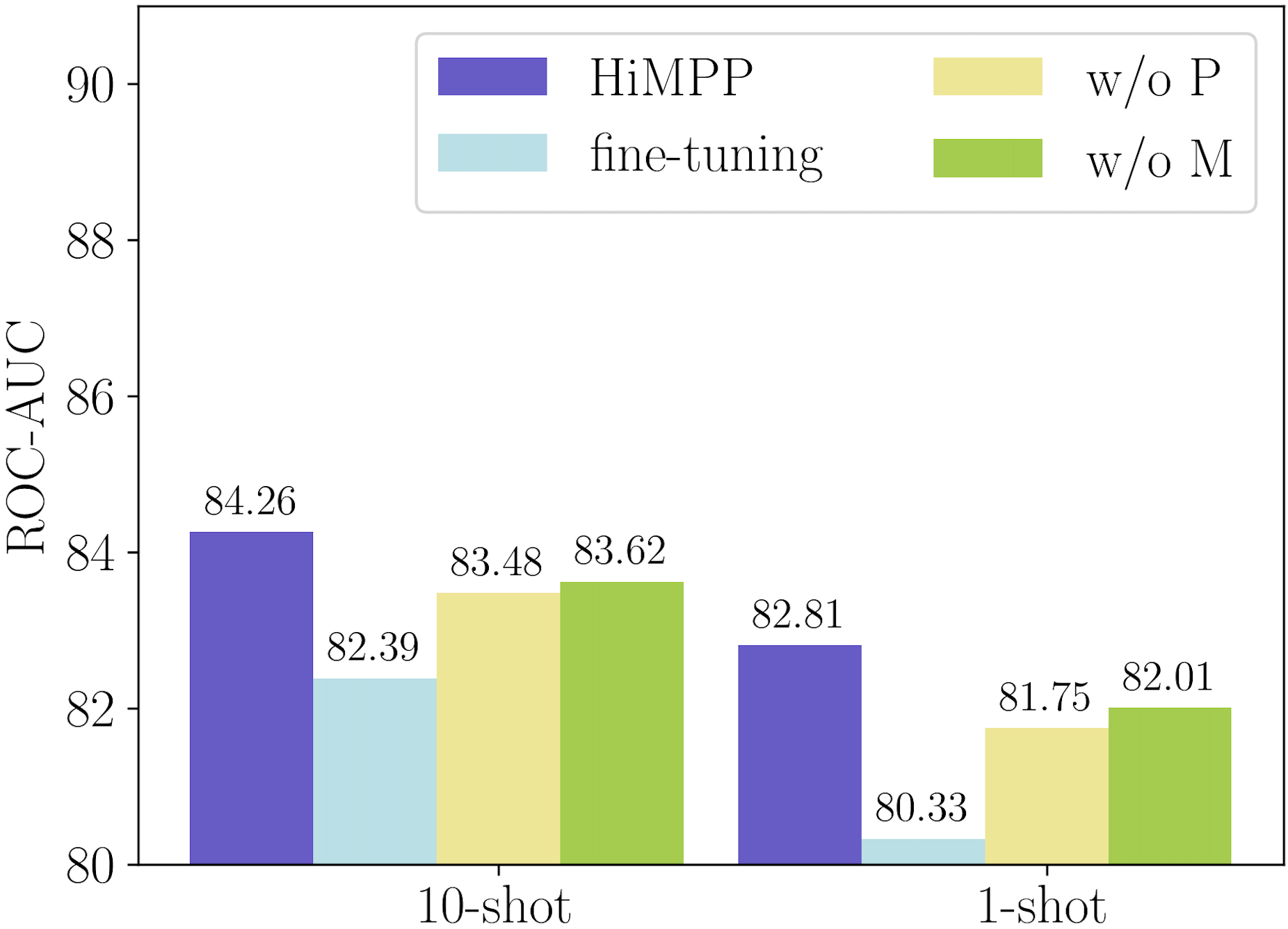
(a) Without pre-training.

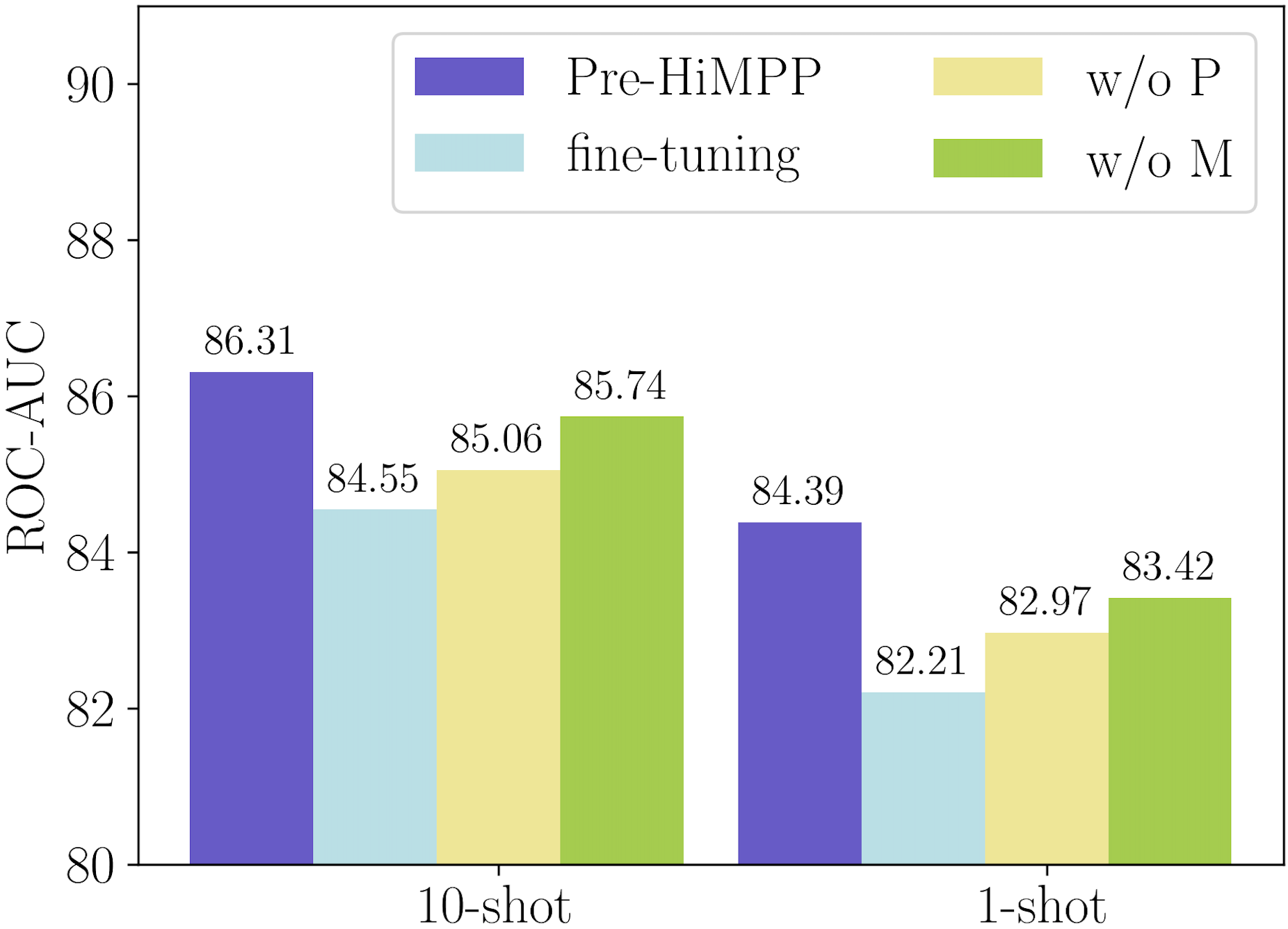
(b) With pre-training.

Figure 2: Ablation study on Tox21.

Table 3: Comparison of property-level adaptation approaches.

	HiMPP	PAR
Total parameters	3.28M	2.31M
Adaptive parameters	3.00K	0.38M
Adaptation steps	-	1	2	3	4	5
Testing ROC-AUC	84.26	82.07	81.85	80.32	79.09	77.25
Time (secs)	1.09	2.02	3.62	5.34	6.76	8.10

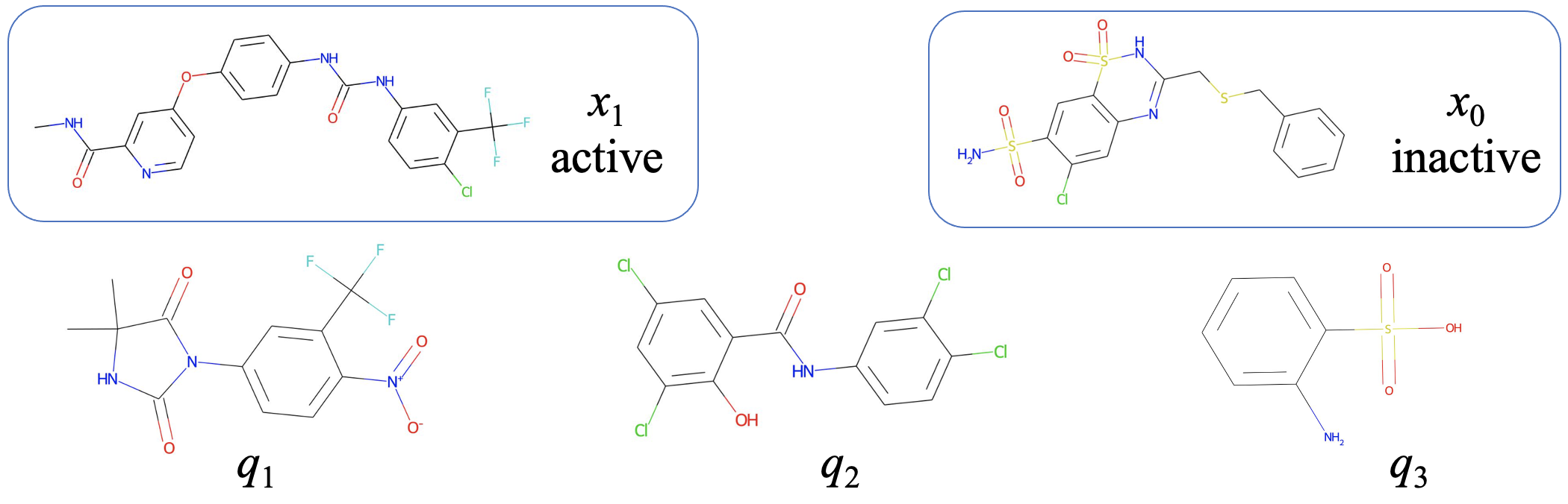
Figure 3: Molecular graphs of $x_{1},~{}x_{0}$ and $q_{1},~{}q_{2},~{}q_{3}$.

Table 4: Illustration of molecule-level adaptation. Classifying $q_{1}$ and $q_{3}$ is relatively easy and the dynamic propagation will take 1 step, while classifying $q_{2}$ is hard and takes 4 steps.

Molecule	$q_{1}$		$q_{2}$		$q_{3}$
	$x_{1}$	$x_{0}$	$x_{1}$	$x_{0}$	$x_{1}$	$x_{0}$
Cosine similarity	0.183	-0.024	0.278	0.252	-0.031	0.129
$t^{\prime}$	1		4		1

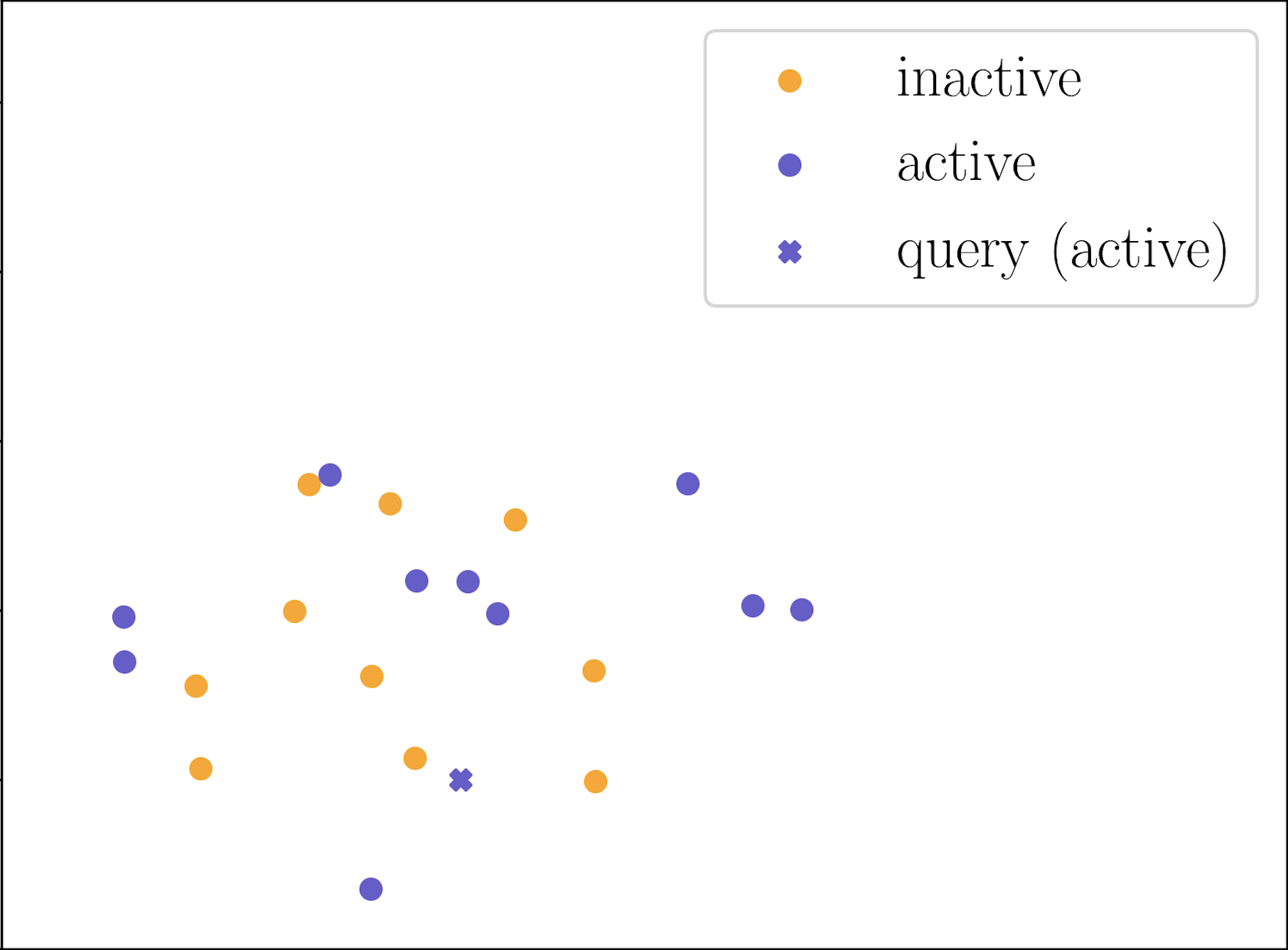
(a) Without adaptation.

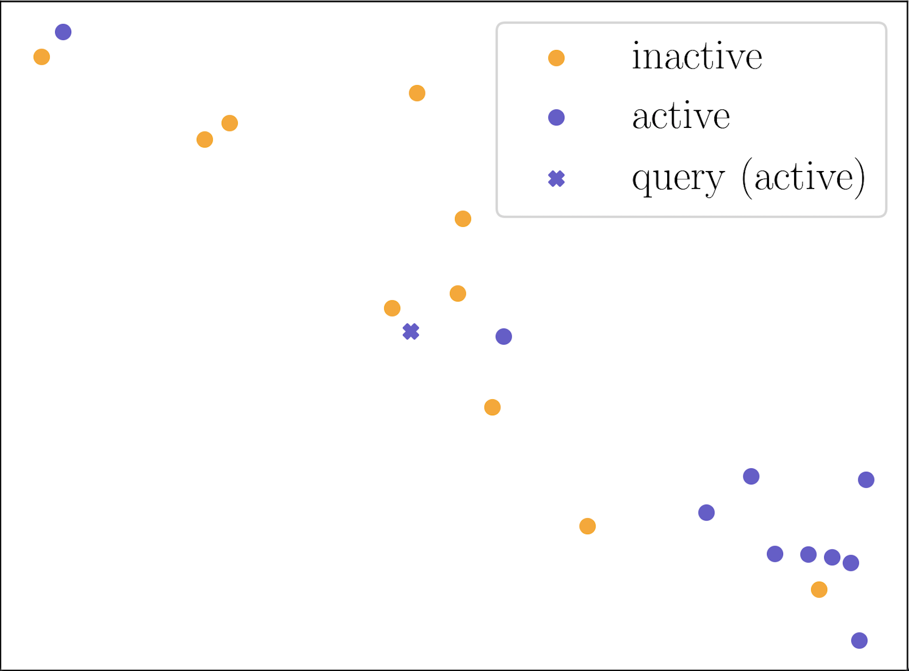
(b) Property-level adaptation.

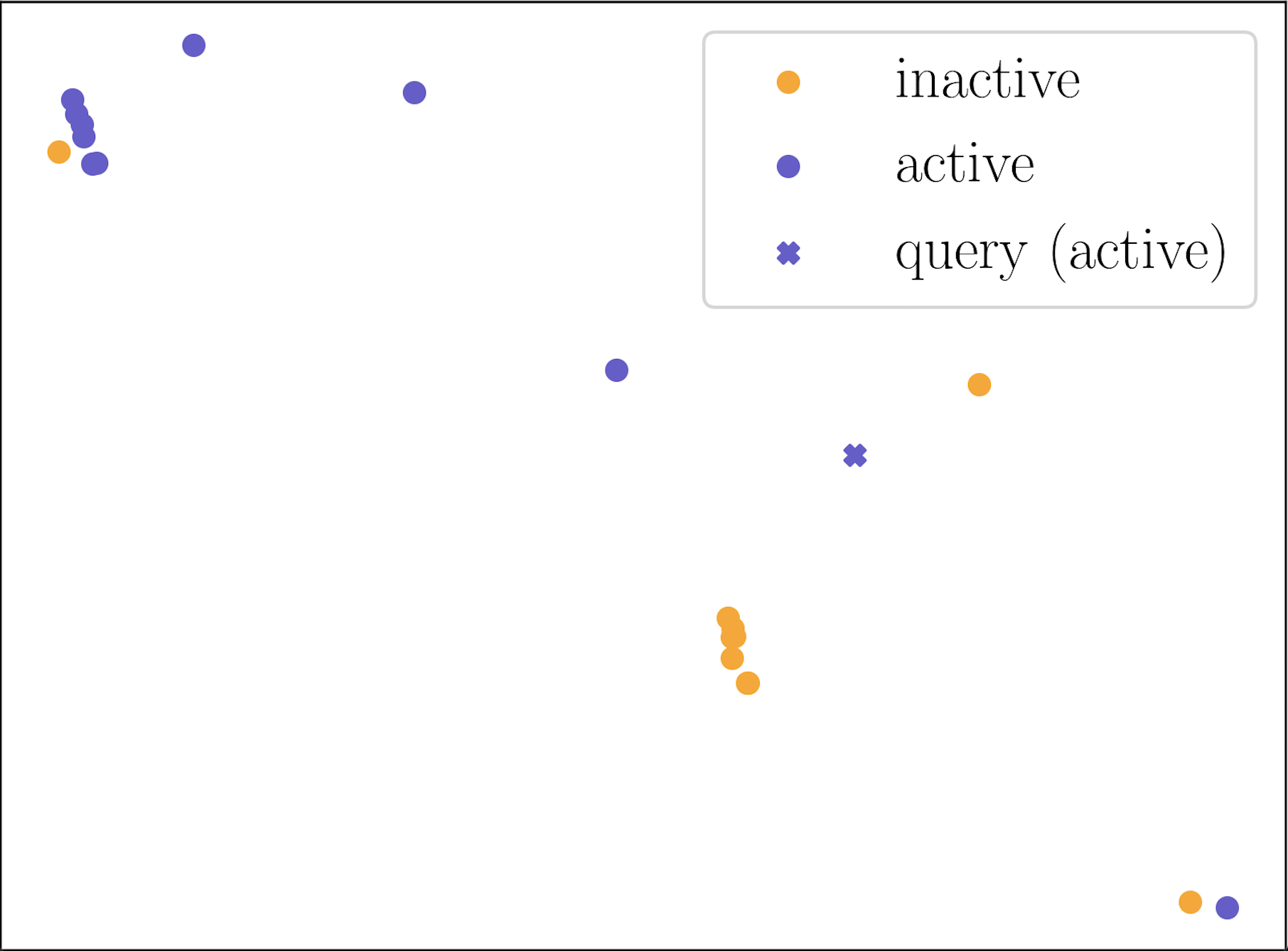
(c) With relation graph.

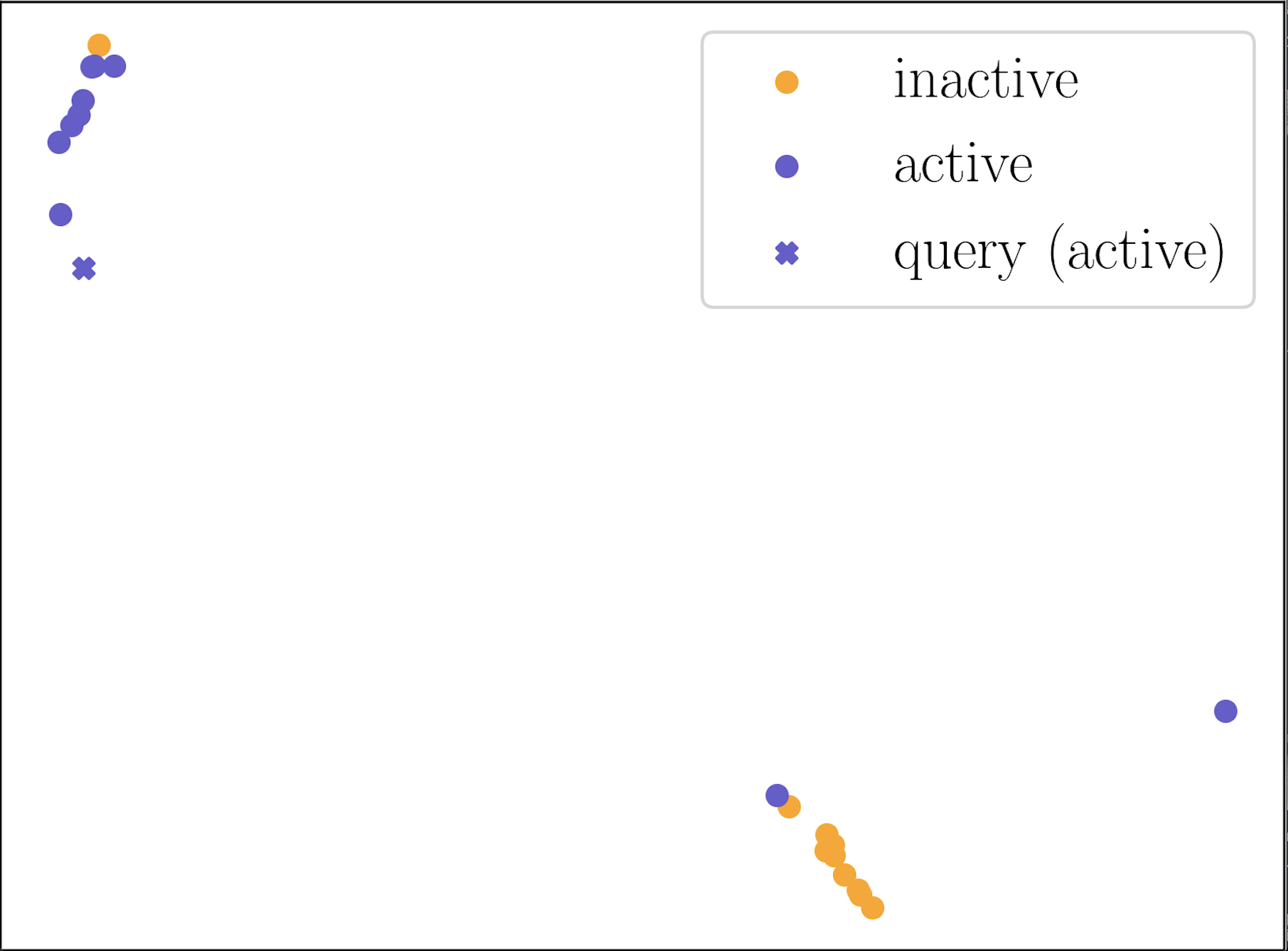
(d) molecule-level adaptation.

Figure 4: Molecular representation visualization for 10-shot case in task SR-p53 of Tox21.

4.2 Ablation Study

We consider various variants of HiMPP and Pre-HiMPP to study the effectiveness of adaptation on each level, including (i) fine-tuning: the same model structure but without hypernetworks and the whole model will be fine-tuned for each property, (ii) w/o P: without property-level adaptation (Section 3.3.1), thus the GNN encoder will not be adapted by the hypernetwork for each property; (iii) w/o M: without molecule-level adaptation (Section 3.3.2), that all molecules are processed by the same number of relation graph layers.

Figure 2 shows the results on Tox21. Observations are as follows: (i) The performance gain of HiMPP over “w/o M" shows the necessity of molecule-level adaptation; (ii) The gap between HiMPP and “w/o P" indicates the effect of our design of hypernetwork-based property-adaptive GNN; (iii) One can also notice that without molecule-level adaptation, “w/o M" still obtains better performance than MAML-based baselines like PAR, which indicates the effectiveness of selectively adapting parameters with hypernetwork; and (iv) The poor performance of “fine-tuning" is possibly because of the over-fitting caused by updating all parameters with only few samples. In summary, every component of HiMPP is important to obtaining good performance.

Figure 4 shows the t-SNE visualization (Van der Maaten and Hinton, 2008) of molecular representations learned on a 10-shot support set and a query molecule with ground truth label “active" in task SR-p53 of Tox21. As shown, molecular representations obtained using pre-trained encoder without adaptation (Figure 4(a)) are mixed up, since the encoder has not been adapted to the target property of the task. Molecular representations being processed by our property-adaptive GNN encoder (Figure 4(b)) becomes more distinguishable, indicating that adapting molecular representation in property-level takes effect. Molecular representations in Figure 4(c) and Figure 4(d) form clear clusters as we encourage similar molecules to be connected during relation graph refinement by (4). The difference is that molecular representations in Figure 4(c) are refined by the best step number for all tasks in 10-shot case, while molecular representations in Figure 4(d) are refined by 4 steps which are selected for the specific query molecule. As shown, we can conclude that our molecular-adaptive refinement steps help better separate molecules of different classes.

4.3 A Closer Look at Property-level Adaptation

To make effective property-level adaptation, we design hypernetwork for encoder to modulate the node embeddings during message passing. We compared our hypernetwork-based adaptation with gradient-based adaptation in PAR which achieved second best performance. The results are shown in Table 3. We record their adaptation process, i.e., there time consumption to process the support set and the test performance. PAR uses the molecules in support set to take gradient steps, and update all parameters in GNN. We record each of a maximum five steps, where we can find that it over-fits easily as the performance keep dropping with more than one step. Also, the time consumption grows. HiMPP processes molecules in support set with hypernetwork, which is much more efficient as only one forward-propagation is needed. HiMPP can achieve better performance since the introduce of shared hypernetwork and the reduction of adaptive parameters (model weights which are variable across tasks) together result in greater generalization and mitigate over-fitting the few shot.

4.4 A Closer Look at Molecular-level Adaptation

We first experiment to show the necessity and effectiveness of the proposed molecule-level adaptation by dynamic propagation. The results are shown in Appendix B.4. Here, we present a case study to illustrate the molecule-level adaptation in a straightforward way. We show a 1-shot support set and 3 query molecules in task SR-p53 of Tox21. In Figure 3, $x_{1}$ and $x_{0}$ are support molecules with different labels, $q_{1}$, $q_{2}$ and $q_{3}$ are query molecules. Considering the shared substructures (function groups), $q_{1}$ and $x_{1}$ are visually similar, $q_{3}$ and $x_{0}$ are visually similar. While both $x_{1}$ and $x_{0}$ share substructures with $q_{2}$, it is hard to tell which of them is more similar to $q_{2}$. In Table 4, we further calculate the cosine similarity based on the molecule representations generated by Pre-GNN , and confirm our observation: $q_{1}$ is much more similar to $x_{1}$, $q_{3}$ is much more similar to $x_{0}$, and $q_{2}$ has close similarities with the both samples. Intuitively, $q_{1}$ and $q_{3}$ will be easier to classify while $q_{2}$ will be hard. In the dynamic propagation of HiMPP, we find different steps are taken: $t^{\prime}=1$ for both $q_{1}$ and $q_{3}$ while $t^{\prime}=4$ for $q_{2}$. HiMPP makes effective molecule-level adaptation by assigning more complex models for molecules that are difficult to classify.

5 Conclusion

We make more accurate few-shot MPP by selectively adapt parameter on property-level and introduce molecule-level adaptation. This is achieved by designing hypernetworks effect on a encoder-predictor MPP model. In the property-adaptive encoder, we select a small amount of parameters in GNN to be adapted via using a hypernetwork to map the support set to FiLM parameters. In the molecule-adaptive predictor, a relation graph is equipped with dynamic propagation, controlled by another hypernetwork which can infer the optimal refinement steps for each specific query molecule. Empirical results show our method obtains state-of-the-art performance on few-shot MPP problem and the effectiveness of our hypernetworks and adaptation mechanism.

Appendix A Method

A.1 Main Network in Property-Adaptive Encoder

As the main network of the encoder, to process a molecule with GNN, each node embedding $\mathbf{h}_{v}$ represents an atom, and each edge $e_{vu}$ represents a chemical bond. Here, we use GIN (Xu et al., 2019) as the main network in encoder, which is a powerful GNN structure. In GIN, the update function in (1) is specified as adding all neighbors up:

$$\mathbf{h}_{\text{agg}}^{l-1}=\sum\nolimits_{\mathcal{H}(v)}\mathbf{h}_{\text{u}}^{l-1}.$$ (11)

As for the update function in (2), we add the aggregated embeddings and the target node, then feed to a MLP:

$$\mathbf{h}_{v}^{l}=\texttt{MLP}^{l}_{G}\left((1+\epsilon)\mathbf{h}_{v}^{l-1}+\mathbf{h}_{\text{agg}}^{l-1}\right),$$ (12)

where $\epsilon$ is a scalar parameter to distinguish the target node. To obtain the molecular representation, the readout function in (3) is specified as

$$\mathbf{r}=\texttt{MLP}_{L}\left(\text{MEAN}(\{\mathbf{h}_{v}^{T}|v\in\mathcal{V}\})\right).$$ (13)

A.2 Classifier in Molecular-Adaptive Predictor

The classifier needs to make prediction of the query $\hat{\mathbf{r}}_{{\tau},q}^{{t}}$, according to the other $2K$ labeled support samples $\{(\hat{\mathbf{r}}_{{\tau},i}^{{t}},y_{{\tau},i})~{}|~{}\mathcal{X}_{{\tau},i}\in\mathcal{S}_{\tau}\}$. We adopt an adaptive classifier (Requeima et al., 2019), which map the labeled samples in each class to the parameters of a linear classifier, i.e.,

$$\bm{w}_{\pm}\!=\!\texttt{MLP}_{w}\Big{(}\frac{1}{|\mathcal{S}_{\tau}^{\pm}|}\!\!\sum\nolimits_{\mathcal{X}_{{\tau},i}\in\mathcal{S}_{\tau}^{\pm}}\hat{\mathbf{r}}_{{\tau},i}^{t}\Big{)},~{}b_{\pm}\!=\!\texttt{MLP}_{b}\Big{(}\frac{1}{|\mathcal{S}_{\tau}^{\pm}|}\!\!\sum\nolimits_{\mathcal{X}_{{\tau},i}\in\mathcal{S}_{\tau}^{\pm}}\hat{\mathbf{r}}_{{\tau},i}^{t}\Big{)},$$

where $\bm{w}_{\pm}$ has the same dimension with $\hat{\mathbf{r}}_{{\tau},q}^{{t}}$, and $b_{\pm}$ is a scalar. Then the prediction is made by

$$\hat{\bm{y}}_{{\tau},q}^{t}=\texttt{softmax}([\bm{w}_{-}^{\top}\hat{\mathbf{r}}_{{\tau},q}^{{t}}+b_{-},~{}\bm{w}_{+}^{\top}\hat{\mathbf{r}}_{{\tau},q}^{{t}}+b_{+}]),$$ (14)

where $\texttt{softmax}(\bm{x})=\text{exp}(\mathbf{x})/\sum\nolimits_{i}\text{exp}\left([\bm{x}]_{i}\right)$ and $[\bm{x}]_{i}$ means the $i$th element in $\bm{x}$.

A.3 Adopting MAML for Property-Level Adaptation

Denote all model parameter as $\bm{\Theta}$. The model first predict samples in support set and get loss to do local-update. Denote the loss for local-update as $\mathcal{L}_{\tau}^{S}(\bm{\Theta})=\sum\nolimits_{\mathcal{X}_{{\tau},i}\in\mathcal{S}_{\tau}}\bm{y}_{{\tau},i}^{\top}\text{log}\left(\hat{\bm{y}}_{{\tau},i}\right)$, where $\hat{\bm{y}}_{{\tau},i}$ is the prediction made by the main network with parameter $\bm{\Theta}$. The loss for global-update is calculated with samples in query set, denoted as , $\mathcal{L}_{\tau}^{Q}(\bm{\Theta}^{\prime}_{\tau})=\sum\nolimits_{\mathcal{X}_{{\tau},i}\in\mathcal{Q}_{\tau}}\bm{y}_{{\tau},i}^{\top}\text{log}\left(\hat{\bm{y}}_{{\tau},i}\right)$, where $\hat{\bm{y}}_{{\tau},i}$ is the prediction made by the main network with parameter $\bm{\Theta}^{\prime}_{\tau}$. Then Algorithm 3 can be adopted for meta-training, and Algorithm 4 for meta-testing.

Algorithm 3 Meta-training with MAML

0:  meta-training task set $\bm{\mathcal{T}}_{\text{train}}$

1:  initialize $\bm{\Theta}$ randomly;

2:  while not done do

3:     for each task $\mathcal{T}_{\tau}\in\bm{\mathcal{T}}_{\text{train}}$ do

4:        evaluate $\nabla_{\bm{\Theta}}\mathcal{L}_{\tau}^{S}(\bm{\Theta})$ with respect to all samples in $\mathcal{S}_{\tau}$;

5:        compute adapted parameters with gradient descent: $\bm{\Theta}^{\prime}_{\tau}=\bm{\Theta}-\nabla_{\bm{\Theta}}\mathcal{L}_{\tau}^{S}(\bm{\Theta})$;

6:     end for

7:     update $\bm{\Theta}\leftarrow\bm{\Theta}-\nabla_{\bm{\Theta}}\sum\nolimits_{\mathcal{T}_{\tau}\in\bm{\mathcal{T}}_{\text{train}}}\mathcal{L}_{\tau}^{Q}(\bm{\Theta}^{\prime}_{\tau})$;

8:  end while

9:  return  learned $\bm{\Theta}^{*}$.

Algorithm 4 Meta-testing with MAML

0:  learned $\bm{\Theta}*$, a meta-testing task $\mathcal{T}_{\tau}$;

1:  evaluate $\nabla_{\bm{\Theta}}\mathcal{L}_{\tau}^{S}(\bm{\Theta})$ with respect to all samples in $\mathcal{S}_{\tau}$;

2:  compute adapted parameters with gradient descent: $\bm{\Theta}^{\prime}_{\tau}=\bm{\Theta}-\nabla_{\bm{\Theta}}\mathcal{L}_{\tau}^{S}(\bm{\Theta})$;

3:  make prediction $\bm{y}_{{\tau},i}$ for $\mathcal{X}_{{\tau},i}\in\mathcal{Q}_{\tau}$ with adapted parameter $\bm{\Theta}^{\prime}_{\tau}$;

A.4 Comparison with Existing Works

We compare the proposed HiMPP with existing few-shot MPP approaches in Table 5. As shown, we manage to compare in perspectives of support of pre-training, property-level adaptation mechanism, molecule-level adaptation mechanism. fast-adaptation and few-shot learning model. With the help of hypernetworks, our method not only introduces novel molecule-level adaptation, but also can adapt on property-level more effectively and efficiently, which can be supported by empirical results in the next section.

Table 5: Comparison of the proposed HiMPP with existing few-shot MPP methods.

Method	Support	Hierarchical adaptation		Fast	Few-shot learning
	Pre-training	Property-level	molecule-level	adaptation	model
IterRefLSTM	$\times$	$\surd$	$\times$	$\surd$	Matching network
Meta-MGNN	$\surd$	$\surd$	$\times$	$\times$	MAML
PAR	$\surd$	$\surd$	$\times$	$\times$	Attention+MAML
HiMPP	$\surd$	$\surd$	$\surd$	$\surd$	Hypernetwork

From the perspective of hypernetwork, the usage of the hypernetwork for encoder is related to GNN-FiLM (Brockschmidt, 2020), which considers a GNN as main network. It builds hypernetwork with target node as input to generate parameters of FiLM layers, to equip different nodes with different aggregation functions in the GNN. What and how to adapt are similar to ours, but it is different that the input of our hypernetwork for encoder is $\mathcal{S}_{\tau}$ and how we encode a set of labeled graphs.

In few-shot learning, some recent works (Requeima et al., 2019; Lin et al., 2021) use hypernetworks to process the task context to make the model task-adaptive. Their hypernetworks have similar functionality of our hypernetwork for encoder, that are used to map the support set to parameter to modulate the main network, but their main networks are convolutional neural network (CNN) and MLP respectively, there is significant difference about what to modulate. As for the usage of the hypernetwork for predictor, which is used to evaluate an unlabeled sample with a set of labeled ones to encode model architecture, did not appear in the literature.

Appendix B Experiments

B.1 Datasets

We perform experiments on four datasets: Tox21 (National Center for Advancing Translational Sciences, 2017), SIDER (Kuhn et al., 2016), MUV (Rohrer and Baumann, 2009) and ToxCast (Richard et al., 2016), which are included in MoleculeNet (Wu et al., 2018). We adopt the task splits provided by existing works(Altae-Tran et al., 2017; Wang et al., 2021). Tox21 is a collection of nuclear receptor assays related to human toxicity, containing 8014 compounds in 12 tasks, among which 9 are split for training and 3 are split for testing. SIDER collects information about side effects of marketed medicines, and it contains 1427 compounds in 21 tasks, among which 21 are split for training and 6 are split for testing. MUV contains compounds designed to be challenging for virtual screening for 17 assays, containing 93127 compounds in 17 tasks, among which 12 are split for training and 5 are split for testing. ToxCast collects compounds with toxicity labels, containing 8615 compounds in 617 tasks, among which 450 are split for training and 167 are split for testing.

B.2 Baselines

We compare our method with following baselines:

• Siamese (Koch et al., 2015): It learns two neural networks which are symmetric on structure to identity whether the input molecule pairs are from the same class. The performance is copied from (Altae-Tran et al., 2017) due to the lack of code.

• ProtoNet (Snell et al., 2017): It makes classification according to inner-product similarity between the target and the prototype of each class. This method is incorporated as a classifier after the GNN encoder.

• MAML (Finn et al., 2017): It learns a parameter initialization and the model is adapted to each task via few gradient steps on the support set. We adopt this method for all parameters in a model composed of a GNN encoder and a linear classifier.

• EGNN (Kim et al., 2019): It builds a relation graph that samples are refined, and it learns to predict edge-labels in the relation graph. This method is incorporated as the predictor after the GNN encoder.

• GNN-FiLM(Brockschmidt, 2020): GNN-FiLM has built hypernetwork with target node as input to generate parameters of FiLM layers, which equips different nodes with different aggregation functions in the GNN. We adopt this as encoder and a MLP as classifier and train on all samples in meta-training tasks and samples in support set of all meta-testing tasks;

• IterRefLSTM (Altae-Tran et al., 2017): It introduces matching networks combined with long short-term memory (LSTM) to refine the molecular representations according to the task context. The performance is copied from (Altae-Tran et al., 2017) due to the lack of code.

• PAR (Wang et al., 2021): It introduces an attention mechanism to capture task-dependent property and an inductive relation graph between samples, and incorporates MAML to train.

• Pre-GNN (Hu et al., 2019): It trains a GNN encoder on ZINC15 dataset with graph-level and node-level self-supervised tasks, and fine-tunes the pre-trained GNN on downstream tasks. We adopt the pre-trained GNN encoder and a linear classifier.

• GraphLoG (Xu et al., 2021): It introduces hierarchical prototypes to capture the global semantic clusters. And adopts an online expectation-maximization algorithm to learn. We adopt the pre-trained GNN encoder and a linear classifier.

• MGSSL (Hu et al., 2019): It trains a GNN encoder on ZINC15 dataset with graph-level, node-level and motif-level self-supervised tasks, and fine-tunes the pre-trained GNN on downstream tasks. We adopt the pre-trained GNN encoder and a linear classifier.

• GraphMAE (Hou et al., 2022): It presents a masked graph autoencoder for generative self-supervised graph pre-training and focus on feature reconstruction with both a masking strategy and scaled cosine error. We adopt the pre-trained GNN encoder and a linear classifier.

• Meta-MGNN (Guo et al., 2021): It incorporates self-supervised tasks such as bond reconstruction and atom type prediction to be jointly optimized via MAML. It uses the pre-trained GNN encoder provided by (Hu et al., 2019).

• Pre-PAR: The same as PAR but uses the pre-trained GNN encoder provided by (Hu et al., 2019).

B.3 Parameter Setting

Here we provide the detailed parameter setting of HiMPP. The maximum layer number of the GNN $L=5$, the maximum steps of the relation graph $T=5$, During training, for each layer in GNN, we set dropout rate as 0.5 operated between the graph operation and FiLM layer. The dropout rate of $\text{MLP}_{L}$ is 0.1. For all baselines on all datasets, we use Adam optimizer (Kingma and Ba, 2015) with learning rate 0.006 and the maximum episode number is 25000. In each episode, the meta-training tasks are learned one-by-one, query set size $M=16$. The ROC-AUC is evaluated every 10 epochs on meta-testing tasks and the best performance is reported. Table 6 shows the details of the other parts. Experiments are conducted on a 24GB NVIDIA GeForce RTX 3090 GPU, with Python 3.8.13, CUDA version 11.7, Torch version 1.10.1.

Table 6: Details of model structure.

	Layers	Output Dimension
$\texttt{MLP}_{E}^{l}$	input $\frac{1}{|\mathcal{V}_{{\tau},i}|}\sum\nolimits_{v\in\mathcal{X}_{{\tau},i}}\big{[}\mathbf{h}_{v}^{l}~{}|~{}\bm{y}_{{\tau},i}\big{]},$, fully connected, LeakyReLU	300
	fully connected with with residual skip connection,$\frac{1}{K}[\sum\nolimits_{\mathcal{X}_{{\tau},i}\in\mathcal{S}_{\tau}^{+}}(\cdot)~{}|~{}\sum\nolimits_{\mathcal{X}_{{\tau},i}\in\mathcal{S}_{\tau}^{-}}(\cdot)]$	300
	fully connected with residual skip connection	300
$\texttt{MLP}_{P}$	input $\{[\bm{r}_{{\tau},i}^{t}~{}|~{}\bm{y}_{{\tau},i}]\}_{\mathcal{S}_{\tau}}$, fully connected, LeakyReLU	128
	2$\times$ (fully connected with with residual skip connection, LeakyReLU)	128
	fully connected with with residual skip connection,$\frac{1}{K}[\bm{r}_{{\tau},q}^{t}~{}|~{}\sum\nolimits_{\mathcal{X}_{{\tau},i}\in\mathcal{S}_{\tau}^{+}}(\cdot)~{}|~{}\sum\nolimits_{\mathcal{X}_{{\tau},i}\in\mathcal{S}_{\tau}^{-}}(\cdot)]$	128
	fully connected, LeakyReLU	256
	fully connected with residual skip connection, LeakyReLU	256
	fully connected	1
$\texttt{MLP}_{G}^{l}$	input $(1+\epsilon)\mathbf{h}_{v}^{l-1}+\mathbf{h}_{\text{agg}}^{l-1}$, fully connected, ReLU	600
	fully connected	300
$\texttt{MLP}_{L}$	input $\texttt{READOUT}\left(\{\mathbf{h}_{v}^{T}|v\in\mathcal{V}_{t,i}\}\right)$, fully connected, LeakyReLU	128
	fully connected	128
$\texttt{MLP}_{A}$	input $\text{exp}(|\mathbf{r}_{{\tau},i}^{t-1}-\mathbf{r}_{{\tau},i}^{t-1}|)$, fully connected, LeakyReLU	256
	fully connected, LeakyReLU	128
	fully connected	1
$\texttt{MLP}_{N}$	input $\mathbf{A}_{\tau}^{t}\bm{R}_{{\tau},q}^{{t}-1}$, fully connected, LeakyReLU	256
	fully connected, LeakyReLU	128
$\texttt{MLP}_{w}$	input $\frac{1}{K}\sum_{y_{{\tau},i}=c}\bm{r}_{{\tau},i}^{t}$, fully connected with residual skip connection, LeakyReLU	128
	2$\times$ (fully connected with residual skip connection, LeakyReLU)	128
	fully connected	128
$\texttt{MLP}_{b}$	input $\frac{1}{K}\sum_{y_{{\tau},i}=c}\bm{r}_{{\tau},i}^{t}$, fully connected with residual skip connection, LeakyReLU	128
	2$\times$ (fully connected with residual skip connection, LeakyReLU)	128
	fully connected	1

B.4 A Closer Look at Molecule-level Adaptation

In this section, we pay a closer look at our molecule-level adaptation mechanism, proving evidence of its effectiveness.

B.4.1 Performance under Different Refinement Steps

Figure 5 compares Pre-HiMPP with “w/o M" (introduced in Section 4.2) using different fixed steps of relation graph refinement on Tox21, where the maximum step number $T=5$. As can be seen, Pre-HiMPP equipped performs much better than “w/o M" which takes the same steps of relation graph refinement as in PAR. This validates the necessity of molecule-level adaptation.

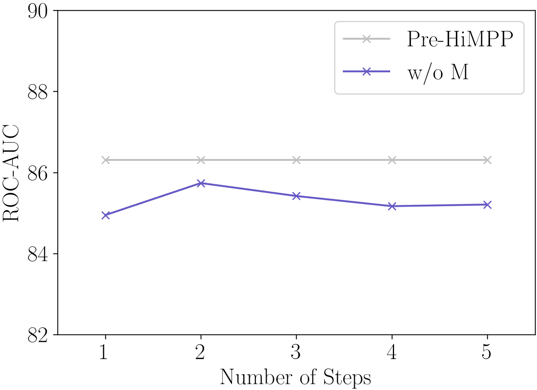
(a) 10-shot case.

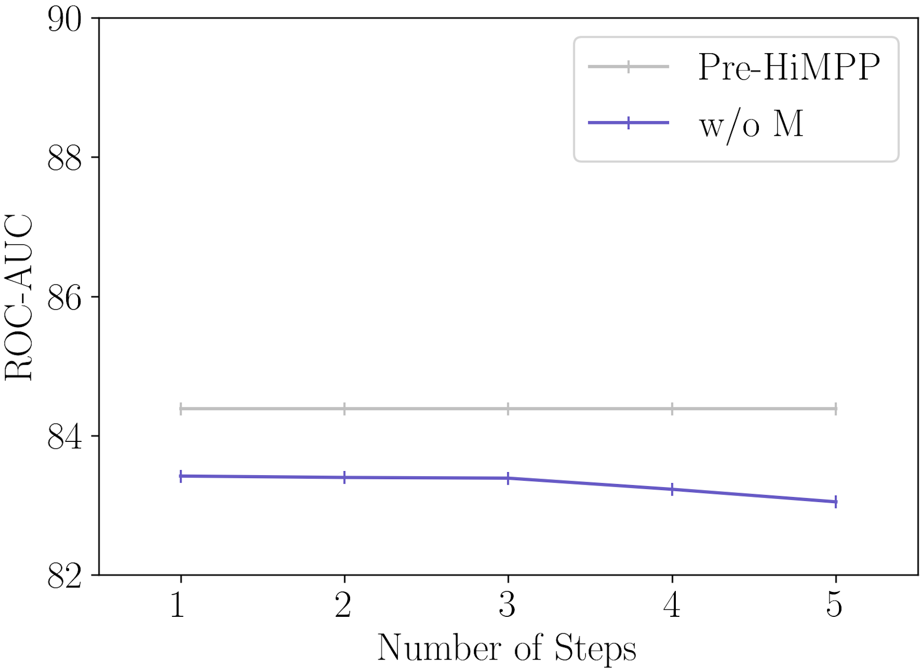
(b) 1-shot case.

Figure 5: Comparing Pre-HiMPP with “w/o M" using different fixed steps of relation graph refinement on Tox21.

B.4.2 Distribution of Refinement Steps

Figure 6(a) plots the distribution of learned $t^{\prime}$ for query molecules in meta-testing tasks for 10-shot case of Tox21. The three meta-testing tasks contain different number of query molecules in scale: 6447 in task SR-HSE, 5790 in task SR-MMP, and 6754 in task SR-p53. We can see that Pre-HiMPP choose different $t^{\prime}$ for query molecules in the same task. Besides, the distribution of learned $t^{\prime}$ varies across different meta-testing tasks: molecules in task SR-MPP mainly choose smaller step numbers while molecules in the other two tasks tend to choose larger step numbers. This can be explained as most molecules in task SR-MPP are relatively easy to classify, which is consistent with the fact that Pre-HiMPP obtains the highest ROC-AUC on SR-MPP among the three meta-testing tasks (83.75 for SR-HSE, 88.79 for SR-MPP and 86.39 for SR-p53).

Further, we pick out molecules with $t^{\prime}=1$ (denote as Group A) and $t^{\prime}=4$ (denote as Group B) as they are more extreme cases. We then apply “w/o M" with different fixed steps for Group A and Group B, and compare them with Pre-HiMPP. Figure 6(b) shows the results. Different observations can be made for these two groups. Molecules in Group A have good performance with fewer steps of relation graph refinement, they can achieve higher ROC-AUC score than the average of all molecules using Pre-HiMPP. These indicate they are easier to classify and it is reasonable that Pre-HiMPP choose $t^{\prime}=1$ for them. While molecules in Group B are harder to classify and requires $t^{\prime}=4$.

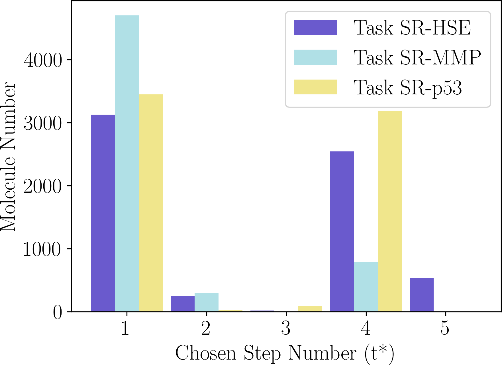
(a) Distribution of learned $t^{\prime}$.

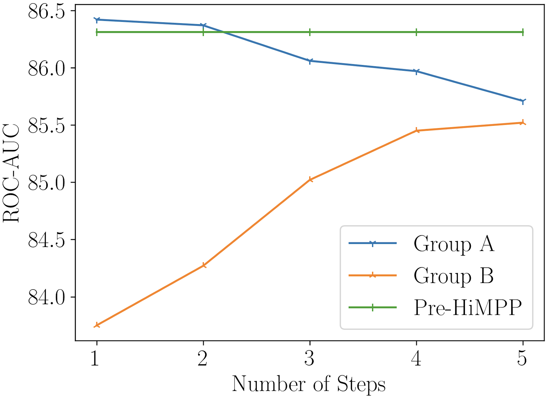
(b) Performance comparison.

Figure 6: Examine the molecule-level adaptation mechanism of Pre-HiMPP using 10-shot case of Tox21.

References

- (1)
- Altae-Tran et al. (2017) Han Altae-Tran, Bharath Ramsundar, Aneesh S Pappu, and Vijay Pande. 2017. Low data drug discovery with one-shot learning. ACS Central Science 3, 4 (2017), 283–293.
- Bengio et al. (2009) Yoshua Bengio, Jérôme Louradour, Ronan Collobert, and Jason Weston. 2009. Curriculum learning. In International Conference on Machine Learning. 41–48.
- Brock et al. (2018) Andrew Brock, Theodore Lim, James M Ritchie, and Nick Weston. 2018. SMASH: One-shot model architecture search through hypernetworks. In International Conference on Learning Representations.
- Brockschmidt (2020) Marc Brockschmidt. 2020. GNN-FiLM: Graph neural networks with feature-wise linear modulation. In International Conference on Machine Learning. 1144–1152.
- Finn et al. (2017) Chelsea Finn, Pieter Abbeel, and Sergey Levine. 2017. Model-agnostic meta-learning for fast adaptation of deep networks. In International Conference on Machine Learning. 1126–1135.
- Garcia and Bruna (2018) Victor Garcia and Joan Bruna. 2018. Few-shot learning with graph neural networks. In International Conference on Learning Representations.
- Guo et al. (2021) Zhichun Guo, Chuxu Zhang, Wenhao Yu, John Herr, Olaf Wiest, Meng Jiang, and Nitesh V Chawla. 2021. Few-Shot Graph Learning for Molecular Property Prediction. In The Web Conference. 2559–2567.
- Ha et al. (2017) David Ha, Andrew Dai, and Quoc V Le. 2017. Hypernetworks. In International Conference on Learning Representations.
- Hou et al. (2022) Zhenyu Hou, Xiao Liu, Yuxiao Dong, Chunjie Wang, Jie Tang, et al. 2022. GraphMAE: Self-Supervised Masked Graph Autoencoders. In ACM SIGKDD International Conference on Knowledge Discovery & Data Mining. 594–604.
- Hu et al. (2019) Weihua Hu, Bowen Liu, Joseph Gomes, Marinka Zitnik, Percy Liang, Vijay Pande, and Jure Leskovec. 2019. Strategies for Pre-training Graph Neural Networks. In International Conference on Learning Representations.
- Kim et al. (2019) Jongmin Kim, Taesup Kim, Sungwoong Kim, and Chang D Yoo. 2019. Edge-labeling graph neural network for few-shot learning. In IEEE/CVF Conference on Computer Vision and Pattern Recognition. 11–20.
- Kingma and Ba (2015) Diederik P Kingma and Jimmy Ba. 2015. Adam: A method for stochastic optimization. In International Conference on Learning Representations.
- Koch et al. (2015) Gregory Koch, Richard Zemel, and Ruslan Salakhutdinov. 2015. Siamese neural networks for one-shot image recognition. In ICML Deep Learning Workshop.
- Kuhn et al. (2016) Michael Kuhn, Ivica Letunic, Lars Juhl Jensen, and Peer Bork. 2016. The SIDER database of drugs and side effects. Nucleic Acids Research 44, D1 (2016), D1075–D1079.
- Li et al. (2018) Ruoyu Li, Sheng Wang, Feiyun Zhu, and Junzhou Huang. 2018. Adaptive graph convolutional neural networks. In AAAI Conference on Artificial Intelligence. 3546–3553.
- Lin et al. (2021) Xixun Lin, Jia Wu, Chuan Zhou, Shirui Pan, Yanan Cao, and Bin Wang. 2021. Task-adaptive neural process for user cold-start recommendation. In The Web Conference. 1306–1316.
- Liu et al. (2022) Shengchao Liu, Hanchen Wang, Weiyang Liu, Joan Lasenby, Hongyu Guo, and Jian Tang. 2022. Pre-training Molecular Graph Representation with 3D Geometry. In International Conference on Learning Representations.
- Ma et al. (2015) Junshui Ma, Robert P Sheridan, Andy Liaw, George E Dahl, and Vladimir Svetnik. 2015. Deep neural nets as a method for quantitative structure–activity relationships. Journal of Chemical Information and Modeling 55, 2 (2015), 263–274.
- Nachmani and Wolf (2020) Eliya Nachmani and Lior Wolf. 2020. Molecule property prediction and classification with graph hypernetworks. arXiv preprint arXiv:2002.00240 (2020).
- National Center for Advancing Translational Sciences (2017) National Center for Advancing Translational Sciences. 2017. Tox21 Challenge. http://tripod.nih.gov/tox21/challenge/. Accessed: 2016-11-06..
- Perez et al. (2018) Ethan Perez, Florian Strub, Harm De Vries, Vincent Dumoulin, and Aaron Courville. 2018. FiLM: Visual reasoning with a general conditioning layer. In AAAI Conference on Artificial Intelligence. 3942–3951.
- Przewiezlikowski et al. (2022) Marcin Przewiezlikowski, P Przybysz, Jacek Tabor, Maciej Zieba, and Przemyslaw Spurek. 2022. HyperMAML: Few-shot adaptation of deep models with hypernetworks. arXiv preprint arXiv:2205.15745 (2022).
- Rajeswaran et al. (2019) Aravind Rajeswaran, Chelsea Finn, Sham M Kakade, and Sergey Levine. 2019. Meta-learning with implicit gradients. In Advances in Neural Information Processing Systems. 113–124.
- Rashid et al. (2018) Tabish Rashid, Mikayel Samvelyan, Christian Schroeder, Gregory Farquhar, Jakob Foerster, and Shimon Whiteson. 2018. QMIX: Monotonic value function factorisation for deep multi-agent reinforcement learning. In International Conference on Machine Learning. PMLR, 4295–4304.
- Requeima et al. (2019) James Requeima, Jonathan Gordon, John Bronskill, Sebastian Nowozin, and Richard E Turner. 2019. Fast and flexible multi-task classification using conditional neural adaptive processes. In Advances in Neural Information Processing Systems. 7957–7968.
- Richard et al. (2016) Ann M Richard, Richard S Judson, Keith A Houck, Christopher M Grulke, Patra Volarath, Inthirany Thillainadarajah, Chihae Yang, James Rathman, Matthew T Martin, John F Wambaugh, et al. 2016. ToxCast chemical landscape: Paving the road to 21st century toxicology. Chemical Research in Toxicology 29, 8 (2016), 1225–1251.
- Rogers and Hahn (2010) David Rogers and Mathew Hahn. 2010. Extended-connectivity fingerprints. Journal of Chemical Information and Modeling 50, 5 (2010), 742–754.
- Rohrer and Baumann (2009) Sebastian G Rohrer and Knut Baumann. 2009. Maximum unbiased validation (MUV) data sets for virtual screening based on PubChem bioactivity data. Journal of Chemical Information and Modeling 49, 2 (2009), 169–184.
- Sitzmann et al. (2020) Vincent Sitzmann, Julien Martel, Alexander Bergman, David Lindell, and Gordon Wetzstein. 2020. Implicit neural representations with periodic activation functions. Advances in Neural Information Processing Systems 33 (2020), 7462–7473.
- Snell et al. (2017) Jake Snell, Kevin Swersky, and Richard Zemel. 2017. Prototypical networks for few-shot learning. In Advances in Neural Information Processing Systems. 4080–4090.
- Stärk et al. (2022) Hannes Stärk, Dominique Beaini, Gabriele Corso, Prudencio Tossou, Christian Dallago, Stephan Günnemann, and Pietro Liò. 2022. 3D infomax improves gnns for molecular property prediction. In International Conference on Machine Learning. PMLR, 20479–20502.
- Sterling and Irwin (2015) Teague Sterling and John J Irwin. 2015. ZINC 15–Ligand discovery for everyone. Journal of Chemical Information and Modeling 55, 11 (2015), 2324–2337.
- Unterthiner et al. (2014) Thomas Unterthiner, Andreas Mayr, Günter Klambauer, Marvin Steijaert, Jörg K Wegner, Hugo Ceulemans, and Sepp Hochreiter. 2014. Deep learning as an opportunity in virtual screening. In NIPS Deep Learning Workshop, Vol. 27. 1–9.
- Van der Maaten and Hinton (2008) Laurens Van der Maaten and Geoffrey Hinton. 2008. Visualizing data using t-SNE. Journal of Machine Learning Research 9, 11 (2008).
- Wang et al. (2021) Yaqing Wang, Abulikemu Abuduweili, Quanming Yao, and Dejing Dou. 2021. Property-aware relation networks for few-shot molecular property prediction. In Advances in Neural Information Processing Systems. 17441–17454.
- Waring et al. (2015) Michael J Waring, John Arrowsmith, Andrew R Leach, Paul D Leeson, Sam Mandrell, Robert M Owen, Garry Pairaudeau, William D Pennie, Stephen D Pickett, Jibo Wang, et al. 2015. An analysis of the attrition of drug candidates from four major pharmaceutical companies. Nature Reviews Drug discovery 14, 7 (2015), 475–486.
- Wieder et al. (2020) Oliver Wieder, Stefan Kohlbacher, Mélaine Kuenemann, Arthur Garon, Pierre Ducrot, Thomas Seidel, and Thierry Langer. 2020. A compact review of molecular property prediction with graph neural networks. Drug Discovery Today: Technologies 37 (2020), 1–12.
- Wu et al. (2018) Zhenqin Wu, Bharath Ramsundar, Evan N Feinberg, Joseph Gomes, Caleb Geniesse, Aneesh S Pappu, Karl Leswing, and Vijay Pande. 2018. MoleculeNet: A benchmark for molecular machine learning. Chemical Science 9, 2 (2018), 513–530.
- Xiong et al. (2019) Zhaoping Xiong, Dingyan Wang, Xiaohong Liu, Feisheng Zhong, Xiaozhe Wan, Xutong Li, Zhaojun Li, Xiaomin Luo, Kaixian Chen, Hualiang Jiang, et al. 2019. Pushing the boundaries of molecular representation for drug discovery with the graph attention mechanism. Journal of Medicinal Chemistry 63, 16 (2019), 8749–8760.
- Xu et al. (2019) Keyulu Xu, Weihua Hu, Jure Leskovec, and Stefanie Jegelka. 2019. How powerful are graph neural networks?. In International Conference on Learning Representations.
- Xu et al. (2021) Minghao Xu, Hang Wang, Bingbing Ni, Hongyu Guo, and Jian Tang. 2021. Self-supervised graph-level representation learning with local and global structure. In International Conference on Machine Learning. 11548–11558.
- Yang et al. (2019) Kevin Yang, Kyle Swanson, Wengong Jin, Connor Coley, Philipp Eiden, Hua Gao, Angel Guzman-Perez, Timothy Hopper, Brian Kelley, Miriam Mathea, et al. 2019. Analyzing learned molecular representations for property prediction. Journal of Chemical Information and Modeling 59, 8 (2019), 3370–3388.
- Yin et al. (2020) Mingzhang Yin, George Tucker, Mingyuan Zhou, Sergey Levine, and Chelsea Finn. 2020. Meta-learning without memorization. In International Conference on Learning Representations.
- Zhang et al. (2021) Zaixi Zhang, Qi Liu, Hao Wang, Chengqiang Lu, and Chee-Kong Lee. 2021. Motif-based graph self-supervised learning for molecular property prediction. In Advances in Neural Information Processing Systems. 15870–15882.