BLACK-BOX ATTACKS ON IMAGE ACTIVITY PREDICTION AND ITS NATURAL LANGUAGE EXPLANATIONS

Abstract

Explainable AI (XAI) methods aim to describe the decision process of deep neural networks. Early XAI methods produced visual explanations, whereas more recent techniques generate multimodal explanations that include textual information and visual representations. Visual XAI methods have been shown to be vulnerable to white-box and gray-box adversarial attacks, with an attacker having full or partial knowledge of and access to the target system. As the vulnerabilities of multimodal XAI models have not been examined, in this paper we assess for the first time the robustness to black-box attacks of the natural language explanations generated by a self-rationalizing image-based activity recognition model. We generate unrestricted, spatially variant perturbations that disrupt the association between the predictions and the corresponding explanations to mislead the model into generating unfaithful explanations. We show that we can create adversarial images that manipulate the explanations of an activity recognition model by having access only to its final output.

1 Introduction

Deep neural models are generally black-box systems whose decision-making process is obscure. Explainable artificial intelligence (XAI) aims to make decisions of deep neural models transparent, i.e. understandable by a human [4]. An XAI model provides insights into the decision-making process identifying feature importance contribution that facilitates error analysis and the identification of uncertain cases. XAI systems favor the assessment of the vulnerabilities of a model [2] and interactions with people to support their decisions [26].

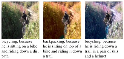
Figure 1: Sample adversarial images generated against NLX-GPT [47] from a clean image (left) by changing the activity prediction while maintaining the textual explanation (middle) and by maintaining the activity prediction while changing the textual explanation (right).

XAI approaches may generate visual (V-XAI), textual (T-XAI) or multimodal (M-XAI) explanations. Visual explanations highlight the most relevant pixel information used by the model [46, 49, 55]. Examples include super-pixels based visualizations (e.g. LIME [46]), heatmaps [49], saliency maps [55], and feature contribution methods inspired by game theory (e.g. SHAP [35]). However, V-XAI outputs may be difficult to comprehend for non-expert users when no information is provided on how highlighted pixels influence the decision. Textual explanations describe the reasons for a decision in a more human-interpretable form through natural language [14, 21, 25, 33, 36]. Finally, multimodal explanations jointly generate textual rationales and visual evidence in the form of attention maps [41, 47, 65]. A recent self-rationalizing M-XAI method [47] simultaneously predicts the decision and justifies, textually and visually, what led to that decision.

Various studies have addressed the vulnerability of V-XAI methods to adversarial attacks [3, 15, 18, 22, 27, 59, 56], however no previous work explicitly considered T-XAI or M-XAI models.

In this paper we present a black-box, content-based and unrestricted attack against a natural language XAI model for image classification [47]. We generate the adversarial attack against a vision-language model with unrestricted semantic colorization. Our attack uses only the final output, namely the textual output or/and the visual maps of the model to determine the adversarial perturbations. We consider two attack scenarios, namely changing the activity prediction while keeping the textual explanation similar and maintaining the same activity prediction while changing the textual explanation (see Figure 1). To the best of our knowledge, no related work explicitly performs black-box attacks on the prediction-generation mechanism of a natural language-based explanation system.

In summary, our contributions are as follows:

• We propose the first black-box attack against the prediction-explanation mechanism of a natural language explanation model for image classification. We evaluate the robustness of the target model against adversarial image colorization techniques under two scenarios: changing the prediction while keeping the explanation similar, and keeping the same prediction while changing the explanation.

• We create adversarial examples by combining image semantics and the information provided by a visual explanation map to localize the most relevant areas for the prediction and to adapt to different image regions.

Table 1: Adversarial attacks against vision-language models. KEY – : white-box, : black-box, : gray-box, T: targeted, $\overline{\text{T}}$: untargeted, R: restricted, $\overline{\text{R}}$: unrestricted, IC: image captioning, SG: story ending text generation, IG: image generation, VQA: visual question answering, ACT-X: activity recognition explanation.

Reference	Task	Box	R	$\overline{\text{R}}$	T	$\overline{\text{T}}$
Chen et al. [10]	IC		✓		✓
Zhang et al. [72]	IC		✓		✓
Ji et al. [24]	IC		✓		✓
Kwon et al. [30]	IC		✓			✓
Xu et al. [68]	IC		✓		✓	✓
Bhattad et al. [7]	IC			✓	✓
Wu et al. [64]	IC	,	✓			✓
Wang et al. [62]	IC	,	✓		✓	✓
Sharma et al. [54]	VQA		✓			✓
Huang et al. [23]	SG		✓			✓
Xu et al. [67]	IC, VQA		✓		✓
Lapid et al. [31]	IC	✓		✓	✓
Aafaq et al. [1]	IC	✓		✓
Chaturvedi et al. [9]	IC, VQA	✓		✓
Zhao et al. [73]	IC, VQA, IG		✓		✓
Ours	ACT-X			✓		✓

2 Related works

V-XAI models are susceptible to adversarial attacks that may, for example, preserve the prediction of the original image but change the explanation [3, 15, 18, 22, 27, 56, 59]. Examples of attacks include restricted adversarial perturbations [18], structured manipulations that change the explanation maps to match an arbitrary target map [15], and adversarial classifiers [56] that fool post-hoc explanations methods such as LIME [46] and SHAP [35]. Other works use simple constant shift transformation of the input data [27], model parameter randomization and data randomization [3], and network fine-tuning with adversarial loss [22] to manipulate visual explanations models.

Table 1 shows a summary of existing attacks on vision-language models. Several studies covered V-XAI methods, however no work has yet explicitly considered textual explanations of self-rationalizing multimodal explanations models. Existing similar research on vision-language models focuses on attacking image captioning or visual question answering models. The attacks use $L_{p}$-norm restricted perturbations and are primarily conducted in a white-box [10, 24, 30, 54, 62, 64, 67, 68, 72] or gray-box [1, 9, 31, 62, 64] setup. These attacks are less practical in a real-world scenario since they require prior knowledge about the victim model, which is not readily available, and are often designed for specific model architectures. Also, restricted perturbations are often not semantically meaningful [38, 57] and can create visible artifacts that can be detected by defenses [16, 53, 66].

Attacks on image-to-text generation models may treat the structured output as a single label and design the attack as a targeted complete sentence [1, 31, 67]. This idea was extended to targeted keywords attacks that encourage the adversarial caption to include a predefined set of keywords in any order [10, 72] or at specified positions in the caption [68]. Methods may mask out targeted keywords while preserving the caption quality for the visual content [24]. Untargeted attacks may use attention maps of the underlying target model to focus the adversarial noise on the regions attended by the model [54]. Generative adversarial models have also been used to create adversarial perturbations [1, 62, 64]. Alternatively, adversarial images may be generated by perturbing an image so that its features resemble those of a target image forcing the model to output the same caption [1, 9, 31].

Multimodal vision-language models for classification tasks are vulnerable to white-box and gray-box adversarial perturbations on a single modality [69] (i.e. image input) or multiple modalities [17, 39, 71] (i.e. image and text input). A multimodal white-box iterative attack [23] that fuses image and text modalities attacks has also been introduced to change the output sentence of a multimodal story-ending generation model. A recent black-box attack [73] deceives large vision-language models assuming a targeted adversarial goal. First, a surrogate model is used to craft adversarial examples with restricted perturbations and transfers the adversarial examples to the victim model; then a query-based attacking strategy generates responses more similar to the targeted text.

In this work, we focus on a self-rationalizing model and empirically analyze the robustness against black-box content-based unrestricted attacks by changing either the activity prediction or the explanation. We do not consider the scenario of attacking both activity and explanation since this would be similar to image-captioning attacks that aim to change the entire textual output of a model. The proposed methodology uses only the final decision of the explanation model and does not rely on any surrogate models. Moreover, considering the attack scenarios, our problem is more challenging since multiple conditions need to be satisfied for an attack to be successful.

3 Methodology

3.1 Problem definition

Let I $\in\mathbb{R}^{h\times w\times 3}$ be an RGB image with height $h$ and width $w$. Let $M_{E}$ be an encoder-decoder M-XAI model such that $M_{E}(I)=\bigl{(}a,e,I_{e}\bigr{)}$, where $a=(a_{1},a_{2},\dots,a_{p})$ represents the generated textual description of the activity and $e=(e_{1},e_{2},\dots,e_{n})$ is the generated textual explanation that justifies the activity decision; $a_{i}$ and $e_{j}$ are words, and $p$ and $n$ are variable sentence lengths, which depend on the type of activity illustrated in the image $I$. The set of possible activities is not fixed if $M_{E}$ uses as decoder a language prediction model that generalizes to activity categories unseen during training. $I_{e}$ is the visual explanation map generated for the predicted activity using the cross-attention weights of $M_{E}$.

We define an adversarial example for the explainable model $M_{E}$, the image $\hat{I}$, such that $M_{E}(\hat{I})=\bigl{(}\hat{a},\hat{e},\hat{I_{e}}\bigr{)}$, where $\hat{a}$, $\hat{e}$, and $\hat{I}_{e}$ are the activity prediction, textual explanation, and visual explanation generated for the image $\hat{I}$. In this work, we focus on the textual explanations and we do not set any conditions on $\hat{I}_{e}$. Under the assumption of faithful explanations (i.e. explanations that accurately reflect the process behind a prediction) the label-rationale should be strongly associated [63]: changing the activity prediction implies a change in its explanation. Therefore, our objective is to break the correlation between activity prediction and its explanation by changing one part while keeping the other unchanged.

We therefore consider two attack scenarios, namely $S1$ for which the activities predictions are different ($a\neq\hat{a}$), but the explanations are similar ($e\simeq\hat{e}$), and $S2$, for which the activities predictions are the same ($a=\hat{a}$), but the explanations are different ($e\nsim\hat{e}$).

3.2 Black-box unrestricted attacks

We condition the perturbation generation on the activity prediction and textual explanation. We craft region-specific unrestricted perturbations and generate adversarial examples following the image semantics-based idea proposed in [52]. To determine the adversarial perturbations we use the (dis)similarity between textual explanations. We consider two strategies for perturbing the semantic areas accordingly and extend them to our problem. The first strategy is a random colorization approach [52] and the second is a strategy that combine photo editing techniques [5].

Explanation similarity. We measure the difference between $e$, the textual explanation generated for the clean image $I$, and $\hat{e}$, the explanation generated for the perturbed image $\hat{I}$. Let $E(\cdot)$ be a transformer-based network [45] that computes the vector embedding of a sentence. Then we calculate the similarity between $e$ and $\hat{e}$, $Q_{\hat{T}}(I,\hat{I})$, as the cosine similarity normalized in the range [0,1]:

$$Q_{\hat{T}}(I,\hat{I})=\frac{1}{2}\left(\frac{\sum_{i=1}^{n}{E(e)_{i}E(\hat{e})_{i}}}{\sqrt{\sum_{i=1}^{n}{{E(e)^{2}_{i}}}}\sqrt{\sum_{i=1}^{n}{{E(\hat{e})^{2}_{i}}}}}+1\right),$$ (1)

where $n$ is the size of the embedding vector. The larger the similarity $Q_{\hat{T}}(I,\hat{I})$, the more similar the explanations for $I$ and $\hat{I}$. For example, let us consider the sentences $e_{1}$: he is standing on a bridge with a backpack on his back, $e_{2}$: he is wearing a backpack and standing on a bridge, and $e_{3}$: he is standing in a field with a frisbee in his hand. Sentences $e_{1}$ and $e_{2}$ have the same meaning and their similarity is 0.97. Sentences $e_{1}$ and $e_{3}$ describe different scenarios (although they share a few words) and their difference is reflected in a lower similarity of 0.69. Sentences $e_{2}$ and $e_{3}$ also have a low similarity of 0.70.

Image partitioning. We use a multi-step segmentation approach to partition an image into sensitive regions, $R_{i}^{s}$, and non-sensitive regions, $R_{j}^{n}$. Sensitive regions correspond to objects whose unrealistic colors and appearance could raise suspicion (e.g. human skin), whereas non-sensitive regions can have their colors arbitrarily modified without necessarily making the image look unnatural. We represent an image $I$ as:

$$I=\bigcup R_{i}^{s}\cup\bigcup R_{j}^{n}.$$ (2)

First, we use semantic segmentation to partition an image into semantic regions, such as person, sky, car, building [11]. Next, we detect skin areas on top of semantic regions representing people and mark the skin as sensitive and unalterable. Finally, we further partition each semantic region into smaller areas and obtain the non-sensitive regions with color-based oversegmentation [32]. An example is shown in Figure 2.

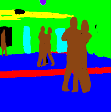
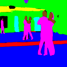
Figure 2: Example of semantic regions obtained after the first step (middle) and last step (right) of the multi-step segmentation scheme. Regions in brown are considered sensitive to color changes.

Optimization process. We find an adversarial example for ${I}$ in $S1$, $\hat{I}_{S1}$, whose generated explanation has the highest similarity with that generated for $I$, while also having a different activity prediction, as follows:

$$\hat{I}_{S1}=\operatorname*{argmax}_{\hat{I}}\bigl{(}Q_{\hat{T}}(I,\hat{I})\mathbbm{1}_{\{(a,\hat{a}):a\neq\hat{a}\}},Q_{\hat{I}}(I,\hat{I})\bigr{)},$$ (3)

where $Q_{\hat{I}}(I,{\hat{I}})$ is used to reduce the noticeability of the perturbation and is implemented as SSIM [61] between the clean image, $I$, and the candidate adversarial example, ${\hat{I}}$, and $\mathbbm{1}_{\{(a,\hat{a}):a\neq\hat{a}\}}$ is the indicator function whose value is 1 only if the predicted activity of $\hat{I}$ is different from the activity of $I$.

Similarly, we find an adversarial example for ${I}$ in $S2$, $\hat{I}_{S2}$, whose generated explanation has the lowest similarity with the explanation generated for the clean image $I$, while also having the same the activity prediction as $I$, as:

$$\hat{I}_{S2}=\operatorname*{argmax}_{\hat{I}}\bigl{(}1-Q_{\hat{T}}(I,\hat{I})\mathbbm{1}_{\{(a,\hat{a}):a=\hat{a}\}},Q_{\hat{I}}(I,\hat{I})\bigr{)},$$ (4)

where $\mathbbm{1}_{\{(a,\hat{a}):a=\hat{a}\}}$ is the indicator function whose value is 1 only if the predicted activity of $\hat{I}$ is the same as the activity of $I$.

Random colorization. We extend ColorFool [52] to consider the explanation similarity $Q_{\hat{T}}$, as defined in Eq. 1. We refer to this method as ColorFoolX (CFX). In this case, we do not use the image similarity $Q_{\hat{I}}$ in the process of finding the adversarial example. We rely only on the image region semantics and prior information about color perception in each region to generate the adversarial images. ColorFool uses the semantic regions computed in the first step of the multi-step segmentation scheme and defines four types of sensitive regions: person, sky, vegetation, and water. Adversarial images are generated by randomly modifying the a and b components of the regions in the perceptually uniform Lab color space within specific color ranges, which depends on the semantics of a region, without changing the lightness L. ColorFool avoids perturbing regions representing people.

Combining editing filters. We extend a combination of image editing filters method [5] to perform localized attention-based attacks. The method manipulates image attributes like saturation, contrast, brightness, sharpness, and applies edge enhancement, gamma correction or soft light gradients. We restrict the perturbations to non-sensitive areas $R_{j}^{n}$ using the information from $I_{e}$: we select the non-sensitive areas that are the most important for the activity prediction, $R_{a}^{n}$, for $S1$, and the least important non-sensitive areas for the activity prediction, $R_{na}^{n}$, for $S2$.

We generate $\hat{I}$, through a sequence of $L$ filters on $I$, for $S1$ as:

$$\hat{I}=R_{i}^{s}\cup f^{\alpha_{t_{1}},\beta_{t_{1}}}_{t_{1}}\circ f^{a_{t_{2}},\beta_{t_{2}}}_{t_{2}}\circ\dots\circ f^{a_{t_{L}},\beta_{t_{L}}}_{t_{L}}(R_{a}^{n})\cup R_{na}^{n},$$ (5)

and for $S2$ as:

$$\hat{I}=R_{i}^{s}\cup R_{a}^{n}\cup f^{\alpha_{t_{1}},\beta_{t_{1}}}_{t_{1}}\circ f^{a_{t_{2}},\beta_{t_{2}}}_{t_{2}}\circ\dots\circ f^{a_{t_{L}},\beta_{t_{L}}}_{t_{L}}(R_{na}^{n}),$$ (6)

where each $f_{i}^{\alpha_{i},\beta_{i}}$ is selected from a set of $F$ predefined filters parameterized with $\beta_{i}$ that controls the amount of change of each property (intensity), and $\alpha_{i}$, the parameter of the alpha blending between the clean image and the filtered image. The optimal filter configuration is found with a nested evolutionary algorithm consisting of an outer optimization step that determines the sequence of $L$ filters with $f_{t_{i}}\in F$ with a genetic algorithm (GA) [37], and an inner optimization step that determines the values of $(\alpha_{t_{i}},\beta_{t_{i}})$ of each selected filter in the outer step with an Evolutionary Strategies (ES) [44].

We consider both $Q_{\hat{T}}$ and $Q_{\hat{I}}$ functions to find the adversarial examples, as defined in Eq. 3, 4. Considering the conflicting nature of the two functions we formulate the optimization process as multi-objective optimization, handled by the NSGA-II algorithm [13], to find the best trade-off between $Q_{\hat{T}}$ and $Q_{\hat{I}}$.

4 Validation

4.1 Experimental setup

Multimodal explanation model. We perform the attacks on the multimodal explanation model NLX-GPT for activity recognition [47], which textually explains its prediction using CLIP [43] as vision encoder and the distilled GPT-2 pre-trained model [48, 8] as a decoder. NLX-GPT generates also a visual explanation map based on the cross-attention weights of the model. The distilled GPT-2 was pre-trained on image-caption pairs (COCO captions [34], Flickr30k [42], visual genome [29] and image-paragraph captioning [28]). NLX-GPT was fine-tuned on the activity recognition dataset ACT-X [41] (18k images). The encoder is fixed for both the pre-training and fine-tuning stages.

Dataset. We use the test set of the ACT-X [41], a 3,620-image dataset used to explain decisions of activity recognition models. Each image is labeled with an activity and three explanations. We perform the attack on the 1,829 images with correctly predicted activity by NLX-GPT.

Cases. We compare different filtering approaches and objective functions. We analyze the following cases: full image filtering (FL-s) and localized filtering (LC-s, as described in Section 3.2) with single objective ($Q_{\hat{T}}$) for explanation (dis)similarity; full image filtering (FL-m) and localized filtering (LC-m) with multi-objective function ($Q_{\hat{T}}$, $Q_{\hat{I}}$), and ColorFoolX (CFX). Note that CFX does not account for image similarity during the attack.

Parameters. For CFX we allow a maximum of 1000 trials. For FL-s and LC-s we follow the CFX iterative approach. For FL-m and LC-m we use the multi-objective evolutionary optimization with the configuration proposed in [5]. We set the size of the outer population to $N_{out}=10$, the number of outer generations to $G_{out}=10$, and the mutation probability to $\rho=0.5$. The inner population size is $\lambda=5$, inner generations $G_{in}=3$ with initial learning rate $lr=0.1$ and decay rate $\beta=0.75$.

4.2 Performance evaluation

Success of the attacks. We measure the success rate, $S_{r}$, of the adversarial attacks as:

$$S_{r}=\frac{1}{N_{a}}\sum\nolimits_{j=1}^{N_{a}}\mathbbm{1}_{\omega},$$ (7)

where $N_{a}$ is the total number of images and, for $S1$:

$$\omega\triangleq\{(a_{j},\hat{a}_{j}):a_{j}\neq\hat{a}_{j}\land Q_{\hat{T}}(I_{j},\hat{I}_{j})\geq t\},$$ (8)

where $t$ is a threshold; and, for $S2$:

$$\omega\triangleq\{(a_{j},\hat{a}_{j}):a_{j}=\hat{a}_{j}\land Q_{\hat{T}}(I_{j},\hat{I}_{j})<t\}.$$ (9)

We determined the value of $t$ with a subjective human evaluation of the similarity of explanations pairs. We created nine groups for the explanations based on their similarity, such that $G_{i}=\{(e,\hat{e}):Q_{\hat{T}}\in(1-0.05i,1-0.05(i-1)]\}$ with $i\in\{1,2,\dots,8\}$ and $G_{9}=\{(e,\hat{e}):Q_{\hat{T}}\in(0,0.6]\}$. From each group, we randomly selected ten $(e,\hat{e})$ pairs that were rated on semantic similarity on a 5-level Likert scale: not similar at all; a little similar; somehow similar; very similar; and they are the same. We used majority voting to assign each pair of explanations to a similarity class. Likewise, we labeled each group with the most frequent similarity class of the questions within the group. Eleven people who did not see the data prior to the test rated the similarity and could change their rating before completing the test. The mapping between explanation groups and similarity classes is shown in Figure 3. We choose somehow similar class as similarity breaking point. This similarity class maps to group G4, which corresponds to $Q_{\hat{T}}<0.85$. Thus, we set the threshold $t=0.85$.

Figure 3: Mapping between explanation groups and similarity classes. KEY – C1: not similar at all, C2: a little similar, C3: somehow similar, C4: very similar, C5: they are the same. Explanations pairs with $Q_{\hat{T}}>0.85$ (i.e. G1-G3) are rated as highly similar.

Image quality. We evaluate the quality of the adversarial images with MANIQA [70], a transformer-based no reference image quality assessment metric that won the NTIRE2022 NR-IQA challenge [19]. MANIQA scores $\in$ [0,1] and the higher the score, the better the quality.

Image colorfulness. We also analyze the colorfulness [20] of the adversarial images and compare it with the colorfulness of original images in order to evaluate whether the colorization attacks generate images with color vividness in accordance with human perception. Given an RGB image, first the opponent color space representation is computed as:

$$rg=R-G,\quad yb=\frac{1}{2}(R+G)-B,$$ (10)

where $R,G,B$ are the red, green, and blue channels. Next, the standard deviation $\sigma$ and the mean pixel values $\mu$ are calculated as:

$$\sigma=\sqrt{\sigma^{2}_{rg}+\sigma^{2}_{yb}},\quad\mu=\sqrt{\mu^{2}_{rg}+\mu^{2}_{yb}}.$$ (11)

Finally, the colorfulness metric is defined as:

$$C=\sigma+0.3\mu.$$ (12)

The higher the $C$ score, the more colorful the image.

Figure 4: Adversarial images generated for a clean image (top left). The visual explanation maps for the activity prediction are shown next to each image. For $S1$ the images have a different activity and the textual explanations are similar. For $S2$ the images have the same activity but different textual explanations. The MANIQA scores for the images are 0.69, 0.63, 0.70, 0.72, 0.64, from top to bottom, respectively.

4.3 Results and Discussion

Success of the attacks. Table 2 reports the success rates for all methods under both scenarios. Methods considering only the explanation similarity (i.e. CFX, FL-s) achieve the best success rate with $S_{r}$ of 64.62% for CFX and 63.09% for FL-s for $S1$, and $S_{r}$ of 73.82 % for CFX and 77.53% for FL-s in $S2$. CFX and FL-s apply the perturbation across wider areas of the image than LC-s, which perturbs small regions selected by combining over-segmentation and visual map information. Moreover, the perturbation is only limited by the semantic region information, which allows more intense modifications than in the case of the multi-objective setup where we use an image similarity metric, $Q_{\hat{I}}$, to calibrate the perturbation. The $S_{r}$ decreases as we focus on more localized areas (LC-s) and as we limit the freedom of the attack with the image similarity function (LC-m). This behavior could be caused by the noisiness and inaccuracy of the cross-attention visual maps, which may fail to accurately explain visually why the model made a certain decision. Since we use the visual maps to localize the areas to attack, inaccurate visual maps lead to selecting areas that are irrelevant for the prediction. These model-intrinsic visual attention maps require more investigation to fully assess their relevance for the localized attacks.

Table 2: Success rate (%) for the two scenarios. KEY – CFX: ColorFoolX, LC-s: localized filtering with a single objective, FL-s: full image filtering with a single objective, LC-m: localized filtering with multi-objective, FL-m: full image filtering with multi-objective.

Scenario	CFX	LC-s	FL-s	LC-m	FL-m
$S1$	64.62	51.33	63.09	43.47	47.62
$S2$	73.82	67.47	77.53	51.76	49.45

We further notice a decrease in attack performance as we enforce an additional constraint on the optimization. On top of the area restriction we also control the applied perturbation using $Q_{\hat{I}}$. Thus, the algorithm has to find a trade-off between explanation (dis)similarity and image similarity. The found solution may sometimes prioritize image similarity over explanation similarity leading to a decrease of the attack success rate. We also notice that the methods are more effective in $S2$ achieving a $S_{r}$ of up to 77.53% for FL-s. In this scenario, the selected alterable areas are more numerous since we focus on regions that are not highly attended by the explanation model, and thus in general the adversarial perturbation is applied on larger image areas than in the case of LC methods. Moreover, we observe that in the case of localized attacks, LC-s and LC-m, the visual attention maps relative to the activity prediction are less noisy and the attention is primarily focused in one area of the image, whereas for CFX more image regions are attended to, similarly to the original image. Localized attacks, for their nature, are more effective in altering the attention of the model.

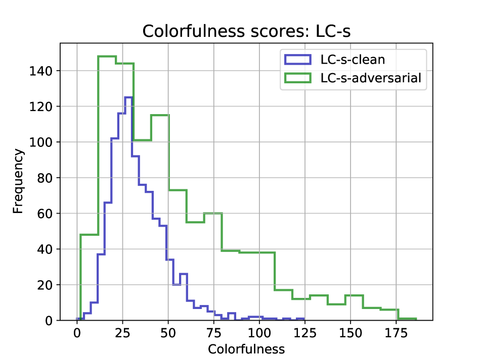
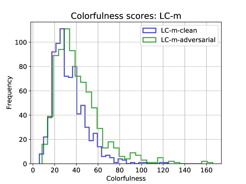
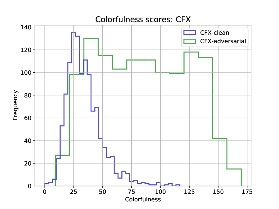
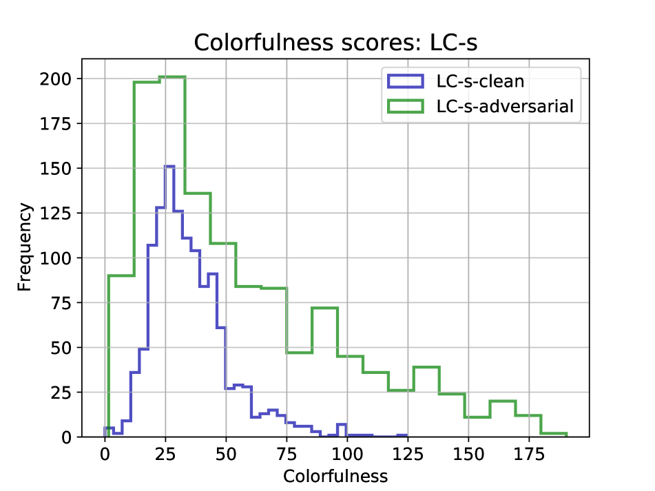
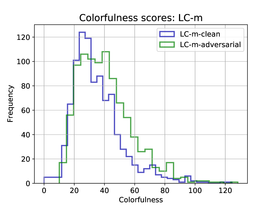
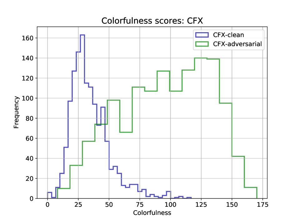
Figure 5: Colorfulness scores distribution for $S1$ (top row) and for $S2$ (bottom row). The adversarial examples generated with LC-m and FL-m have colors similar to the original images. In the case of CFX, the colors of adversarial examples diverge from the distribution of original images. The higher the score, the more colorful the image.

Image quality. Both methods produce comparable results, however, the generated adversarial images have different visual characteristics and aesthetics. In general, the image filtering attacks produce images with more toned-down soft vintage looks while most of the images generated by CFX have vivid colors (see Figure 4). Table 3 reports the average MANIQA and standard deviation scores for the adversarial images and their corresponding clean versions. The average MANIQA score varies from 0.65 for FL-s and LC-s to 0.68 for CFX, LC-m, and FL-m. As a reference, the average score on the clean images is 0.70. This suggests that the adversarial perturbations do not substantially degrade the image quality.

Table 3: Average (and standard deviation) of MANIQA scores for the adversarial images and their corresponding clean images.

	$S1$		$S2$
	Clean	Adversarial	Clean	Adversarial
CFX	.70 $\pm$ .05	.68 $\pm$ .06	.70 $\pm$ .05	.67 $\pm$ .06
LC-s	.69 $\pm$ .05	.66 $\pm$ .06	.70 $\pm$ .04	.65 $\pm$ .07
FL-s	.70 $\pm$ .05	.65 $\pm$ .07	.70 $\pm$ .05	.65 $\pm$ .06
LC-m	.69 $\pm$ .05	.67 $\pm$ .07	.70 $\pm$ .04	.68 $\pm$ .05
FL-m	.70 $\pm$ .05	.66 $\pm$ .07	.70 $\pm$ .05	.68 $\pm$ .05

Image colorfulness. Figure 5 shows the distribution of colorfulness scores of adversarial images and their corresponding original version. LC-m and FL-m generate images with colors most similar to the original images, whereas LC-s and FL-s tend to generate images with more faded colors. This indicates that the image similarity objective contributes toward the generations of more natural-looking images, as also shown by the SSIM scores in Figure 6. On the contrary, CFX generates very colorful images that diverge the most from the original distribution (Figure 5). However, images different from the original ones do not necessarily imply worse quality. Thus, a human subjective evaluation remains the best way to assess the perceptual realism, which we will address in future work.

Ablation study. We perform an ablation study to verify the contribution of each part of the multi-objective function of FL-m and LC-m in both attack success rate and SSIM values (Table 4). We start with a random approach, where we randomly perturb the images while only considering changing the activity prediction, disregarding explanation and image similarity. Then we consider each objective separately. For the image similarity objective, $Q_{\hat{I}}$, the aim is to find the image that changes the activity prediction and has the highest SSIM. For the explanation objective, $Q_{\hat{T}}$, the goal is to find an image that changes the activity prediction and has the highest explanation similarity. When using both objectives, the goal is to find an adversarial image that has a different activity prediction, high explanation similarity and high image similarity. We consider both full image filtering, FL, and localized image filtering, LC. In the case of the image similarity objective only, adversarial images have the highest SSIM scores but a low $S_{r}$. However, the textual explanation objective achieves the highest $S_{r}$ at the expense of the image similarity. This is the main justification for using the version with both objectives to find a trade-off between $S_{r}$ and SSIM.

Table 4: Success rate ($S_{r}$) and structural similarity (SSIM) for different objective functions for $S1$.

Text similarity	Image similarity	LC		FL
		$S_{r}\%$	SSIM	$S_{r}\%$	SSIM
		21.87	.86	22.86	.73
✓		51.33	.73	63.09	.72
	✓	26.93	.95	28.16	.84
✓	✓	43.47	.92	47.62	.84

Figure 6 shows the generally large SSIM values of the adversarial examples obtained with LC-s, FL-s, LC-m, FL-m, and CFX for $S1$. The results show that using SSIM for the optimization of the FL and LC is useful for generating images with higher similarity since the type of modification applied can alter the structural similarity. Among all, CFX generates images with the highest SSIM values because it does not directly target the lightness attribute in the images, which can degrade the structural similarity.

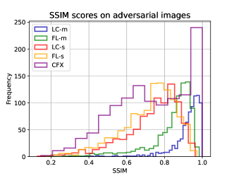
Figure 6: SSIM distribution for $S1$. FL and LC benefit from using the image similarity objective for the optimization. CFX generates images with the highest SSIM values because it does not alter the lightness attribute of the images, which can affect the structural similarity.

We also conducted the analysis for CFX to assess its attack capabilities with respect to the original version of ColorFool (CF) [52]. CFX searches for the adversarial example that satisfies two conditions, while CF only considers the activity prediction. The $S_{r}$ is $\sim$ 80% when we attack only the activity prediction. When considering also the explanation similarity, as in $S1$, CF reaches $S_{r}$ of 37.23 %, whereas CFX reaches $S_{r}$ of 64.62 % (Eq. 7). Similarly, when using FL-s to attack only the activity, we observed that $\sim$ 66% of images with different activity have also different explanations ($Q_{\hat{T}}<0.85$).

5 Conclusion

We presented a black-box attack on a self-rationalizing multimodal explanation system and evaluated the robustness of its prediction-explanation mechanism under two scenarios: changing the activity prediction while keeping the textual explanations similar and preserving the activity prediction while modifying the textual explanation. The adversarial examples are generated through semantic colorization or through image filtering. We showed that the prediction-explanation mechanism is vulnerable to black-box attacks that use only the final output of the target model. As future work, we will conduct a subjective evaluation of the adversarial examples to inform the attention mechanism. The proposed approach could be used to develop model-agnostic evaluation metrics to enable comparative and fair assessment of the faithfulness of different vision-language explanation systems.

References

- [1] Nayyer Aafaq, Naveed Akhtar, Wei Liu, Mubarak Shah, and Ajmal Mian. Language model agnostic gray-box adversarial attack on image captioning. IEEE Trans. on Information Forensics and Security, 2023.
- [2] Amina Adadi and Mohammed Berrada. Peeking inside the black-box: A survey on Explainable Artificial Intelligence (XAI). IEEE Access, 2018.
- [3] Julius Adebayo, Justin Gilmer, Michael Muelly, Ian Goodfellow, Moritz Hardt, and Been Kim. Sanity checks for saliency maps. In Adv. Neural Inf. Process. Syst., 2018.
- [4] Alejandro Barredo Arrieta, Natalia Díaz Rodríguez, et al. Explainable Artificial Intelligence (XAI): Concepts, taxonomies, opportunities and challenges toward responsible AI. Information Fusion, 2020.
- [5] Alina Elena Baia, Gabriele Di Bari, and Valentina Poggioni. Effective universal unrestricted adversarial attacks using a MOE approach. In Int. Conf. Appl. Ev. Comput., 2021.
- [6] Satanjeev Banerjee and Alon Lavie. METEOR: An automatic metric for MT evaluation with improved correlation with human judgments. In Proc. ACL Workshop on Intrinsic and Extrinsic Evaluation Measures for Machine Translation and/or Summarization, 2005.
- [7] Anand Bhattad, Min Jin Chong, Kaizhao Liang, Bo Li, and D. A. Forsyth. Unrestricted adversarial examples via semantic manipulation. In Proc. Int. Conf. on Learning Repr., 2020.
- [8] Tom Brown, Benjamin Mann, Nick Ryder, et al. Language models are few-shot learners. In Adv. Neural Inf. Process. Syst., 2020.
- [9] Akshay Chaturvedi and Utpal Garain. Mimic and Fool: A task-agnostic adversarial attack. IEEE Trans. on Neural Networks and Learning Syst., 2020.
- [10] Hongge Chen, Huan Zhang, Pin-Yu Chen, Jinfeng Yi, and Cho-Jui Hsieh. Attacking visual language grounding with adversarial examples: A case study on neural image captioning. In Proc. of the 56th Annual Meeting ACL, 2018.
- [11] Bowen Cheng, Ishan Misra, Alexander G Schwing, Alexander Kirillov, and Rohit Girdhar. Masked-attention mask transformer for universal image segmentation. In Conf. Comput. Vis. Pattern Recognit., 2022.
- [12] Miruna Clinciu, Arash Eshghi, and Helen Hastie. A study of automatic metrics for the evaluation of natural language explanations. In Conf. of the Eur. Chapter of the ACL, 2021.
- [13] Kalyanmoy Deb, Amrit Pratap, Sameer Agarwal, and T. Meyarivan. A fast and elitist multiobjective genetic algorithm: NSGA-II. IEEE Trans. on Ev. Comput., 2002.
- [14] Virginie Do, Oana-Maria Camburu, Zeynep Akata, and Thomas Lukasiewicz. e-SNLI-VE: Corrected visual-textual entailment with natural language explanations. arXiv:2004.03744 [cs.CL], 2020.
- [15] Ann-Kathrin Dombrowski, Maximillian Alber, Christopher Anders, Marcel Ackermann, Klaus-Robert Müller, and Pan Kessel. Explanations can be manipulated and geometry is to blame. In Adv. Neural Inf. Process. Syst., 2019.
- [16] Gintare Karolina Dziugaite, Zoubin Ghahramani, and Daniel M. Roy. A study of the effect of JPG compression on adversarial images. arXiv:1608.00853v1 [cs.CV], 2016.
- [17] Ivan Evtimov, Russel Howes, Brian Dolhansky, Hamed Firooz, and Cristian Canton Ferrer. Adversarial evaluation of multimodal models under realistic gray box assumption. arXiv:2011.12902 [cs.CV], 2020.
- [18] Amirata Ghorbani, Abubakar Abid, and James Zou. Interpretation of neural networks is fragile. In Proc. AAAI Conf. on Artificial Intell., 2019.
- [19] Jinjin Gu, Haoming Cai, Chao Dong, et al. NTIRE 2022 challenge on perceptual image quality assessment. In Conf. Comput. Vis. Pattern Recognit. Worksh., 2022.
- [20] David Hasler and Sabine E. Suesstrunk. Measuring colorfulness in natural images. In Proc. Int. Society for Optical Engineering, 2003.
- [21] Lisa Anne Hendricks, Zeynep Akata, Marcus Rohrbach, Jeff Donahue, Bernt Schiele, and Trevor Darrell. Generating visual explanations. In Eur. Conf. Comput. Vis., 2016.
- [22] Juyeon Heo, Sunghwan Joo, and Taesup Moon. Fooling neural network interpretations via adversarial model manipulation. In Adv. Neural Inf. Process. Syst., 2019.
- [23] Qingbao Huang, Chuan Huang, Linzhang Mo, Jielong Wei, Yi Cai, Ho-fung Leung, and Qing Li. IgSEG: Image-guided story ending generation. In Findings ACL: Int. J. Conf. on Natural Language Process., 2021.
- [24] Jiayi Ji, Xiaoshuai Sun, Yiyi Zhou, Rongrong Ji, Fuhai Chen, Jianzhuang Liu, and Qi Tian. Attacking image captioning towards accuracy-preserving target words removal. In Proc. ACM Int. Conf. Multimedia, 2020.
- [25] Maxime Kayser, Oana-Maria Camburu, Leonard Salewski, Cornelius Emde, Virginie Do, Zeynep Akata, and Thomas Lukasiewicz. e-ViL: A dataset and benchmark for natural language explanations in vision-language tasks. In Int. Conf. Comput. Vis., 2021.
- [26] Sunnie S.Y. Kim, Elizabeth Anne Watkins, Olga Russakovsky, Ruth Fong, and Andrés Monroy-Hernández. ”Help Me Help the AI ”: Understanding how explainability can support human-AI interaction. In Proc. Conf. Human Factors in Comput. Syst., 2023.
- [27] Pieter-Jan Kindermans, Sara Hooker, Julius Adebayo, Maximilian Alber, Kristof T. Schütt, Sven Dähne, Dumitru Erhan, and Been Kim. The (un)reliability of saliency methods. In Explainable AI: Interpreting, Explaining and Visualizing Deep Learning. 2019.
- [28] Jonathan Krause, Justin Johnson, Ranjay Krishna, and Li Fei-Fei. A hierarchical approach for generating descriptive image paragraphs. In Conf. Comput. Vis. Pattern Recognit., 2017.
- [29] Ranjay Krishna, Yuke Zhu, Oliver Groth, Justin Johnson, Kenji Hata, Joshua Kravitz, Stephanie Chen, Yannis Kalantidis, Li-Jia Li, David A. Shamma, Michael S. Bernstein, and Li Fei-Fei. Visual genome: Connecting language and vision using crowdsourced dense image annotations. Int. J. Comput. Vis., 2017.
- [30] Hyun Kwon and SungHwan Kim. Restricted-area adversarial example attack for image captioning model. Wireless Commun. and Mobile Comput., 2022.
- [31] Raz Lapid and Moshe Sipper. I See Dead People: Gray-box adversarial attack on image-to-text models. arXiv:2306.07591 [cs.CV], 2023.
- [32] Tao Lei, Peng Liu, Xiaohong Jia, Xuande Zhang, Hongying Meng, and Asoke K. Nandi. Automatic fuzzy clustering framework for image segmentation. IEEE Trans. on Fuzzy Syst., 2020.
- [33] Qing Li, Qingyi Tao, Shafiq Joty, Jianfei Cai, and Jiebo Luo. VQA-E: Explaining, elaborating, and enhancing your answers for visual questions. In Eur. Conf. Comput. Vis., 2018.
- [34] Tsung-Yi Lin, Michael Maire, Serge Belongie, James Hays, Pietro Perona, Deva Ramanan, Piotr Dollár, and C. Lawrence Zitnick. Microsoft COCO: Common objects in context. In Eur. Conf. Comput. Vis., 2014.
- [35] Scott M. Lundberg and Su-In Lee. A unified approach to interpreting model predictions. In Adv. Neural Inf. Process. Syst., 2017.
- [36] Ana Marasović, Chandra Bhagavatula, Jae Sung Park, Ronan Le Bras, Noah A. Smith, and Yejin Choi. Natural language rationales with full-stack visual reasoning: From pixels to semantic frames to commonsense graphs. In Findings ACL : EMNLP, 2020.
- [37] Zbigniew Michalewicz. Genetic Algorithms + Data Structures = Evolution Programs. Springer-Verlag, 1992.
- [38] Apostolos Modas, Seyed-Mohsen Moosavi-Dezfooli, and Pascal Frossard. SparseFool: a few pixels make a big difference. In Conf. Comput. Vis. Pattern Recognit., 2019.
- [39] David A. Noever and Samantha E. Miller Noever. Reading Isn’t Believing: Adversarial attacks on multi-modal neurons. arXiv:2103.10480 [cs.LG], 2021.
- [40] Kishore Papineni, Salim Roukos, Todd Ward, and Wei-Jing Zhu. BLEU: A method for automatic evaluation of machine translation. In Proc. Association Comput. Linguistics, 2002.
- [41] Dong Huk Park, Lisa Anne Hendricks, Zeynep Akata, Anna Rohrbach, et al. Multimodal explanations: Justifying decisions and pointing to the evidence. In Conf. Comput. Vis. Pattern Recognit., 2018.
- [42] Bryan A. Plummer, Liwei Wang, Chris M. Cervantes, et al. Flickr30k entities: Collecting region-to-phrase correspondences for richer image-to-sentence models. In Int. Conf. Comput. Vis., 2015.
- [43] Alec Radford, Jong Wook Kim, Chris Hallacy, et al. Learning transferable visual models from natural language supervision. In Proc. Int. Conf. on Machine Learning, 2021.
- [44] Ingo Rechenberg. Evolutionsstrategie: Optimierung technischer systeme nach prinzipien der biologischen evolution. Dr.-Ing. Thesis, Technical University of Berlin, 1971.
- [45] Nils Reimers and Iryna Gurevych. Sentence-BERT: Sentence embeddings using siamese BERT-networks. In Conf. on Empirical Methods in Natural Language Process., 2019.
- [46] Marco Tulio Ribeiro, Sameer Singh, and Carlos Guestrin. ”Why Should I Trust You?”: Explaining the predictions of any classifier. In Proc. ACM SIGKDD Int. Conf. Knowledge Discovery and Data Mining, 2016.
- [47] Fawaz Sammani, Tanmoy Mukherjee, and Nikos Deligiannis. NLX-GPT: A model for natural language explanations in vision and vision-language tasks. In Conf. Comput. Vis. Pattern Recognit., 2022.
- [48] Victor Sanh, Lysandre Debut, Julien Chaumond, and Thomas Wolf. DistilBERT, a distilled version of BERT: smaller, faster, cheaper and lighter. In Adv. Neural Inf. Process. Syst. EMC2 Worksh., 2019.
- [49] Ramprasaath R. Selvaraju, Michael Cogswell, Abhishek Das, Ramakrishna Vedantam, Devi Parikh, and Dhruv Batra. Grad-CAM: Visual explanations from deep networks via gradient-based localization. In Int. Conf. Comput. Vis., 2017.
- [50] Ali Shahin Shamsabadi, Changjae Oh, and Andrea Cavallaro. EdgeFool: An adversarial image enhancement filter. In Proc. IEEE Int. Conf. Acoust., Speech Signal Process., 2019.
- [51] Ali Shahin Shamsabadi, Changjae Oh, and Andrea Cavallaro. Semantically adversarial learnable filters. IEEE Trans. Image Process., 2021.
- [52] Ali Shahin Shamsabadi, Ricardo Sanchez-Matilla, and Andrea Cavallaro. ColorFool: Semantic adversarial colorization. In Conf. Comput. Vis. Pattern Recognit., 2020.
- [53] Mahmood Sharif, Lujo Bauer, and Michael K. Reiter. On the suitability of -norms for creating and preventing adversarial examples. In Conf. Comput. Vis. Pattern Recognit. Worksh., 2018.
- [54] Vasu Sharma, Ankita Kalra, Sumedha Chaudhary Vaibhav, Labhesh Patel, and Louis-Phillippe Morency. Attend and Attack: Attention guided adversarial attacks on visual question answering models. In Adv. Neural Inf. Process. Syst., 2018.
- [55] Karen Simonyan, Andrea Vedaldi, and Andrew Zisserman. Deep inside convolutional networks: Visualising image classification models and saliency maps. arXiv:1312.6034 [cs.CV], 2014.
- [56] Dylan Slack, Sophie Hilgard, Emily Jia, Sameer Singh, and Himabindu Lakkaraju. Fooling LIME and SHAP: Adversarial attacks on post hoc explanation methods. In Proc. AAAI/ACM Conf. on AI, Ethics, and Society, 2020.
- [57] Jiawei Su, Danilo Vasconcellos Vargas, and Kouichi Sakurai. One pixel attack for fooling deep neural networks. IEEE Trans. on Ev. Comput., 2019.
- [58] Liangru Sun, Felix Juefei-Xu, Yihao Huang, Qing Guo, Jiayi Zhu, Jincao Feng, Yang Liu, and Geguang Pu. ALA: Adversarial lightness attack via naturalness-aware regularizations. In Eur. Conf. Comput. Vis. Worksh., 2022.
- [59] J. Vadillo, R. Santana, and J.A. Lozano. When and How to Fool Explainable Models (and Humans) with Adversarial Examples. arXiv:2107.01943 [cs.LG], 2021.
- [60] Yajie Wang, Shangbo Wu, Wenyi Jiang, Shengang Hao, Yu-an Tan, and Quanxin Zhang. Demiguise attack: Crafting invisible semantic adversarial perturbations with perceptual similarity. In Int. J. Conf. on Artificial Intell., 2021.
- [61] Zhou Wang, Alan C. Bovik, Hamid R. Sheikh, and Eero P. Simoncelli. Image quality assessment: From error vsibility to structural similarity. IEEE Trans. Image Process., 2004.
- [62] Zheng Wang, Yang Yang, Jingjing Li, and Xiaofeng Zhu. Universal adversarial perturbations generative network. World Wide Web, 2022.
- [63] Sarah Wiegreffe, Ana Marasović, and Noah A. Smith. Measuring association between labels and free-text rationales. In Conf. on Empirical Methods in Natural Language Process., 2021.
- [64] Hanjie Wu, Yongtuo Liu, Hongmin Cai, and Shengfeng He. Learning transferable perturbations for image captioning. ACM Trans. Multimedia Comput. Commun. Appl., 2022.
- [65] Jialin Wu and Raymond J. Mooney. Faithful multimodal explanation for visual question answering. In Proc. ACL Workshop BlackboxNLP: Analyzing and Interpreting Neural Networks for NLP, 2019.
- [66] Weilin Xu, David Evans, and Yanjun Qi. Feature squeezing: Detecting adversarial examples in deep neural networks. In Network and Distr. Syst. Security Symp., 2018.
- [67] Xiaojun Xu, Xinyun Chen, Chang Liu, Anna Rohrbach, Trevor Darrell, and Dawn Song. Fooling vision and language models despite localization and attention mechanism. In Conf. Comput. Vis. Pattern Recognit., 2018.
- [68] Yan Xu, Baoyuan Wu, Fumin Shen, Yanbo Fan, Yong Zhang, Heng Tao Shen, and Wei Liu. Exact adversarial attack to image captioning via structured output learning with latent variables. In Conf. Comput. Vis. Pattern Recognit., 2019.
- [69] Karren Yang, Wan-Yi Lin, Manash Barman, Filipe Condessa, and Zico Kolter. Defending multimodal fusion models against single-source adversaries. In Conf. Comput. Vis. Pattern Recognit., 2021.
- [70] Sidi Yang, Tianhe Wu, Shuwei Shi, Shanshan Lao, Yuan Gong, et al. MANIQA: Multi-dimension attention network for no-reference image quality assessment. In Conf. Comput. Vis. Pattern Recognit. Worksh., 2022.
- [71] Jiaming Zhang, Qi Yi, and Jitao Sang. Towards adversarial attack on vision-language pre-training models. In Proc. ACM Int. Conf. Multimedia, 2022.
- [72] Shaofeng Zhang, Zheng Wang, Xing Xu, Xiang Guan, and Yang Yang. Fooled by imagination: Adversarial attack to image captioning via perturbation in complex domain. In Proc. IEEE Int. Conf. on Multimedia and Expo, 2020.
- [73] Yunqing Zhao, Tianyu Pang, Chao Du, Xiao Yang, Chongxuan Li, Ngai-Man Cheung, and Min Lin. On evaluating adversarial robustness of large vision-language models. arXiv:2305.16934 [cs.CV], 2023.
- [74] Zhengyu Zhao, Zhuoran Liu, and Martha Larson. Adversarial robustness against image color transformation within parametric filter space. arXiv:2011.06690v2 [cs.CV], 2020.