Schwarzschild Modeling of Barred S0 Galaxy NGC 4371

Abstract

We apply the barred Schwarzschild method developed by Tahmasebzadeh et al. (2022) to a barred S0 galaxy, NGC 4371, observed by IFU instruments from the TIMER and ATLAS3D projects. We construct the gravitational potential by combining a fixed black hole mass, a spherical dark matter halo, and stellar mass distribution deprojected from $3.6$ $\mu$m S⁴G image considering an axisymmetric disk and a triaxial bar. We create two sets of independent models, fitting the kinematic data derived from TIMER and ATLAS3D, separately. The models fit all the kinematic data remarkably well. We find a consistent bar pattern speed from the two sets of models, with $\Omega_{\rm p}=23.6\pm 2.8\hskip 2.27626pt\mathrm{km\hskip 1.13791pts^{-1}\hskip 1.13791ptkpc^{-1}}$. The dimensionless bar rotation parameter is determined to be $\mathcal{R}\equiv R_{\rm cor}/R_{\rm bar}=2.2\pm 0.4$, indicating a slow bar in NGC 4371. Besides, we obtain a dark matter fraction $M_{\rm DM}/M_{\rm total}$ of $\sim 0.51\pm 0.06$ within the bar region. Our results support the scenario that bars may slow down in the presence of dynamical friction with a significant amount of dark matter in the disk regions. Based on our model, we further decompose the galaxy into multiple 3D orbital structures, including a BP/X bar, a classical bulge, a nuclear disk, and a main disk. The BP/X bar is not perfectly included in the input 3D density model, but BP/X-supporting orbits are picked through the fitting to the kinematic data. This is the first time a real barred galaxy has been modeled utilizing the Schwarzschild method including a 3D bar. Our model can be applied to a large number of nearby barred galaxies with IFU data, and it will significantly improve the previous models in which the bar is not explicitly included.

1 Introduction

About two-thirds of disk galaxies in the local universe host bars Eskridge et al. (2000); Erwin (2018). Bars can be detected from non-axisymmetric features in the surface density or from kinematic signatures, e.g., a positive correlation between mean velocity and the third Gauss-Hermite moment $h_{3}$ Bureau & Athanassoula (2005); Li et al. (2018).

The key parameters that characterize a bar are its bar radius, strength, and pattern speed (e.g., Aguerri et al. (2015)). The bar radius and strength can be derived from optical or near-infrared images Aguerri et al. (1998); Buta & Block (2001). The bar pattern speed is a dynamical parameter that requires kinematic measurements and is usually harder to measure. Tremaine & Weinberg (1984) introduced a simple and model-independent method (TW method) for measuring the pattern speed $\Omega_{\rm p}$ of barred galaxies, which is widely used. The TW method uses the profiles of surface brightness $\Sigma(x)$ and line-of-sight (LOS) velocity $V_{los}$ measured along the slits crossing the bar and parallel to the disk major axis, with the coordinate of $x$ integrated from $-\infty$ to $\infty$ along a slit.

In recent decades, integral field unit (IFU) surveys such as SAURON Bacon et al. (2010), CALIFA Sánchez et al. (2012), SAMI Croom et al. (2012), and MaNGA Bundy et al. (2015), have provided kinematic maps of thousands of nearby galaxies. IFU data improves the accuracy of the pattern speed measurement. The TW method has been applied to sub-samples of barred galaxies from CALIFA Aguerri et al. (2015); Cuomo et al. (2019a), MaNGA Guo et al. (2019); Garma-Oehmichen et al. (2022); Géron et al. (2023), and MUSE observed galaxies Cuomo et al. (2019b); Buttitta et al. (2022); Cuomo et al. (2022). The accuracy of the TW method depends on accurately determining the disk position angle. Inaccuracies of a few degrees in the disk position angle can lead to errors of 10% (up to 100%) for $\Omega_{\rm p}$ Debattista (2003); Zou et al. (2019). There is still large uncertainty in the measured pattern speed with MaNGA-like data. MUSE/VLT Bacon et al. (2010) can provide IFU data with higher spatial resolution and S/N, however, accurately measuring $\Omega_{\rm p}$ requires kinematic data covering the bar and the disk’s outer regions, such observations with MUSE are expensive Cuomo et al. (2019b); Buttitta et al. (2022); Cuomo et al. (2022).

Bars can play a significant role in the formation of galaxies by redistributing the energy and the angular momentum of the disk materials Debattista & Sellwood (1998a); Athanassoula (2003); Kormendy & Kennicutt (2004); Gadotti (2011). Many observations and simulations found that bars can be associated with a boxy/peanut or X-shaped (hereafter BP/X) structure in edge-on views Combes & Sanders (1981); Raha et al. (1991); Lütticke et al. (2000). Recently, a sample of 21 nearby barred galaxies have been observed with MUSE on the Very Large Telescope as part of the TIMER project Gadotti et al. (2020), which shows abundant structures in the galaxy center. A bar could co-exist with a classical bulge, a nuclear disk, or a ring-like structure Méndez-Abreu et al. (2014); Erwin et al. (2015). To fully understand the formation of these structures, we need to decompose them in a physical way, thus quantifying their contributions. Besides, the bar pattern speed of most of the TIMER galaxies can not be determined by the TW method, as the data only cover the bar region.

Dynamical modeling is a powerful method that can constrain the bar pattern speed using the full kinematic information, and lead to physical decomposition of the bar, classical bulge, and nuclear disk structures. The bar pattern speed of the Milky Way was strongly constrained by a few dynamical models, including Schwarzschild (1979) orbit-superposition Wang et al. (2013) and Made-to-Measure method Long et al. (2013); Portail et al. (2017). The orbit-superposition method, in particular, the van den Bosch et al. (2008) triaxial code (hereafter VdB08) has been widely used in exploring stellar orbit distribution for a large sample of galaxies from the CALIFA (Zhu et al., 2018a, b), MaNGA (Jin et al., 2020) and SAMI (Santucci et al., 2022). It has been further developed to include the stellar age and metallicity (Zhu et al., 2020; Poci et al., 2019), which leads to chemo-dynamical decomposition of galaxy structures (Zhu et al., 2022; Ding et al., 2023). A new implementation of VdB08 code named DYNAMITE has been publicly released with new features are being Jethwa et al. (2020); Thater et al. (2022).

However, dynamical modeling of external barred galaxies is challenging due to their complicated morphological and kinematic properties. N-body simulations are used as input of the 3D density distribution in the previous barred models, like the triaxial bulge/bar/disk M2M model for M31 Blaña Díaz et al. (2018), and Schwarzschild FORSTAND code Vasiliev & Valluri (2020). Recently, Dattathri et al. (2023) introduced a new method that employs a parametric 3D density distribution to deproject edge-on barred galaxies with BP/X shaped structures. This approach was validated using dynamical modeling against mock data with the FORSTAND code.

In Tahmasebzadeh et al. (2021), we presented a deprojection method to estimate the 3D density distribution of barred galaxies across various observational orientations by including an axisymmetric disk and a triaxial (mostly prolate) bar. We then used these 3D density distributions as input and modified the VdB08 code to include the bar explicitly (Tahmasebzadeh et al., 2022). The testing of the model with mock data demonstrated that we can well recover the barred galaxy’s key properties, particularly the bar pattern speed and boxy-peanut structure.

Here, we apply our bar modeling approach to a real barred galaxy, NGC 4371, which is a particularly interesting galaxy observed by both the TIMER and ATLAS3D projects. This is the first time a real barred galaxy has been modeled utilizing the Schwarzschild method in which the bar is explicitly included. NGC 4371 has complicated inner structures including a nuclear disk, a bar, and it is still controversial whether it has a classical bulge or not (Erwin et al., 2015; Gadotti et al., 2015). The stellar population of the whole galaxy seems very old, and the bar pattern speed is still not determined due to the limited data coverage. By creating an orbit-superposition model, we will quantitatively obtain the contribution of the classical bulge, bar, and nuclear disk and strongly constrain some key parameters including the bar pattern speed.

The paper is organized as follows. In Section 2, we introduce the photometry and spectroscopy data used for modeling. We describe the bar modeling steps and the technical details in Section 3. We present the results and illustrate the key properties of NGC 4371 that we measured in Section 4. We summarize and conclude in Section 5. In the Appendix, we discuss the improvement of our new approach compared to previous axisymmetric models applied to a large sample of spiral galaxies without including the bar in the literature.

2 DATA

2.1 General Properties of NGC 4371

NGC 4371 is a massive early-type galaxy located around the center of the Virgo cluster at a distance of $\sim 16.9$ Mpc Blakeslee et al. (2009). In an early study, Erwin & Sparke (1999) found NGC 4371 has a complex central structure, including a stellar nuclear ring with a $\sim 10$ arcsec radius (1 arcsec $\sim 82$ pc). They suggest that the central structure of this galaxy is dynamically cool and disklike. Buta et al. (2015) classified NGC 4371 as a barred S0 galaxy that shows symmetric enhancements at the ends of the bar, called ansae. They found NGC 4371 has a nuclear ring, a barlens, and a nuclear ring. Fisher & Drory (2010) classified NGC 4371 as a pseudobulge. Erwin et al. (2015) discussed that NGC 4371 hosts a composite bulge, including a small classical merger-built bulge that coexists with a pseudobulge. While Gadotti et al. (2015) did not find evidence for a classical bulge in NGC 4371, they argued it has a nuclear disc and possibly a box/peanut bulge associated with the bar. Detailed analysis of the stellar kinematics showed that the barlens observed in the photometry is a rapidly-rotating nuclear disk Gadotti et al. (2015). NGC 4371 is an old system (older than 7 Gyr throughout), with a slightly younger and more metal-rich population in the nuclear ring Gadotti et al. (2015), and an active and star-forming galactic nucleus Dullo et al. (2016).

Erwin et al. (2008) reported the inclination angle of NGC 4371 to be $58^{\circ}$ and determined the deprojected bar radius $R_{\rm bar}$ with a lower limit of 64 arcsec and upper limit of 75 arcsec using ellipse fits analysis. Gadotti et al. (2015) reported an inclination angle of $60^{\circ}$ with a projected bar semi-major axis of $34.8$ arcsec that indicates a deprotected bar radius of $R_{\rm bar}\sim 70$ arcsec using image decomposition code BUDDA de Souza et al. (2004); Gadotti (2008).

2.2 Photometry

We use the $3.6$ $\mu$m image of NGC 4371 taken by the Infrared Array Camera (IRAC) Channel 1 from the Spitzer Survey of Stellar Structures in Galaxies (S⁴G) Sheth et al. (2010). The pixel size of the S⁴G image is $0.75^{{}^{\prime\prime}}$ and the point spread function (PSF) FWHM is $\approx 1.8^{{}^{\prime\prime}}$ Kim et al. (2014). Because of fewer effects of dust extinction and emission at these wavelengths, the S⁴G image accurately represents the stellar structures in the galaxy. The stellar population of NGC 4371 is generally old in the whole regions covered by MUSE (Gadotti et al., 2015), although the stellar kinematics are derived from MUSE spectroscopy covering the optical band, it should still be safe for us to assume that the S⁴G image traces the light distribution.

2.3 Spectroscopy

NGC 4371 has been observed with MUSE as a part of the TIMER project Gadotti et al. (2019). MUSE covers an almost square $1^{{}^{\prime}}\times 1^{{}^{\prime}}$ field of view (FOV) with contiguous sampling of $0.2^{{}^{\prime\prime}}\times 0.2^{{}^{\prime\prime}}$ and the spectral coverage of $4750-9350$ $\rm\AA$. The spectral sampling is $1.25$ $\rm\AA$ per pixel, and the total integration time is $3840$ s. The stellar kinematics maps of NGC 4371 had been studied in Gadotti et al. (2015, 2020).

To achieve our desired number of stellar kinematic constraints, we re-extract the 2D maps of $v$, $\sigma$, $h_{3}$, and $h_{4}$ from the MUSE data cubes using the Penalized Pixel-Fitting (pPXF) software Cappellari & Emsellem (2004) through the GIST pipeline Bittner et al. (2019). We spatially binned the spectra to ensure a minimum signal-to-residual noise (S/N) of approximately $\sim 140$ per spectral pixel. This was done using the Voronoi binning technique presented by Cappellari & Copin (2003). We consider a minimum S/N threshold of $\sim 3$ for each bin to avoid spaxels with a weak signal leading to outer apertures contamination. The stellar templates are taken from the Medium-resolution Isaac Newton Telescope Library of Empirical Spectra (MILES) stellar library Sánchez-Blázquez et al. (2006); Falcón-Barroso et al. (2011). The MILES stellar templates cover the wavelength range $4760-7400$ $\rm\AA$ and we fit the wavelength range of $4800-7400$ $\rm\AA$ in the galaxy spectrum. We adopt an 8th-order multiplicative polynomial and a 4th-order additive Legendre polynomial.

NGC 4371 is also observed with SAURON Bacon et al. (2001) as part of the volume-limited ATLAS3D project that examined stellar and gas kinematics and photometric imaging of 260 early-type galaxies Cappellari et al. (2011). The SAURON $33^{{}^{\prime\prime}}\times 41^{{}^{\prime\prime}}$ FOV was sampled by $0.94^{{}^{\prime\prime}}\times 0.94^{{}^{\prime\prime}}$ square lenslets in the low resolution mode. So it covers a smaller inner region of NGC 4371 than the MUSE datacube. We downloaded the stellar kinematic datacube provided on the ATLAS3D website which is extracted with the spectral coverage of $4800-5400$ $\rm\AA$.

3 DYNAMICAL MODEL

3.1 Gravitational Potential

We assume a gravitational potential including stellar mass, dark matter (DM), and a central black hole (BH). However, the kinematic data do not resolve the BH sphere of influence. Using velocity dispersion $\sigma_{e}$ within the effective radius $R_{e}$ of the galaxy from Saglia et al. (2016) and $M_{\rm BH}-\sigma_{e}$ relation of Kormendy & Ho (2013), we estimate the NGC 4371 BH to be $\sim 10^{7}M_{\odot}$, whose sphere of influence is $r\sim 0.2^{{}^{\prime\prime}}$, which is smaller than the MUSE PSF. Therefore, we fix the BH mass to be $M_{\rm BH}=10^{6.8}M_{\odot}$ that is measured for NGC 4371 by Saglia et al. (2016) using an axisymmetric model and SINFONI data Bonnet et al. (2003); Eisenhauer et al. (2003). We adopt a spherical Navarro–Frenk–White (NFW) halo Navarro et al. (1996), with one free parameter of dark matter virial mass $M_{200}$, and a fixed concentration $c$ using the correlation between $M_{200}$ and $c$ from (Dutton & Macciò, 2014). The choice of a fixed $c$ will not affect our results significantly because the data are not extended to a large radius, thus, we cannot constrain $c$ and $M_{200}$ simultaneously. The method described here is not tied to the specific parametrization of the DM halo. According to our tests with the mock data in Tahmasebzadeh et al. (2022), the different parametrizations of the DM halo do not alter the results.

3.1.1 Stellar Mass

We create a model for the intrinsic 3D luminosity density of a barred galaxy by deprojecting its 2D photometry image following the method described in Tahmasebzadeh et al. (2021). We first decompose the galaxy image into a disk and a bar, then use multi-Gaussian expansion (MGE) Cappellari (2002) to fit the 2D surface density of the disk and the bar separately, and deproject the disk and the bar allowing different assumptions of their internal 3D shapes. Finally, we obtain the intrinsic 3D luminosity distribution of the whole galaxy by combining the disk and the bar.

The 2D Decomposition:

we use GALFIT Peng et al. (2010) to fit the 2D surface brightness of NGC 4371 with a four-component model including: a central compact Sérsic component, an exponential nuclear disk, a bar (Sérsic profile), and an exponential main disk. The uncertainty of the image is taken from Poisson noise, produced by GALFIT to weight the data points in the fitting. The four-component model fits the data well. We combine the nuclear and main disks as the disk component, then subtract the disk component from the original image to obtain a residual bar. The central compact Sérsic component is considered to reside within the bar. Its notably small effective radius ensures that its presence as part of either the disk or the bar would not influence the results.

Table.1 shows the structural parameters derived from the fit. The right column of Fig.1 shows (from top to bottom) the S⁴G image, GALFIT model, residual, and the bar obtained by subtracting the disk component (nuclear disk + extended disk) from the S⁴G image. The left column of Fig.1 shows (from top to bottom) the radial surface brightness profile derived from the S⁴G image and GALFIT model with ellipse fits to the isophotes, ellipticity, position angle, and the radial surface brightness profile of subcomponents derived from the fit. We determine the projected bar semi-major axis from the GALFIT model to be $R_{\rm bar}^{{}^{\prime}}\sim 35$ arcsec, which is similar to what is reported by Gadotti et al. (2015) using image decomposition. A bump can be seen at this radius in total surface brightness, ellipticity, and position angle profiles. Considering an inclination of $60^{\circ}$, the intrinsic bar radius is $R_{\rm bar}\sim 69$ arcsec ($\sim 5.7$ $\rm kpc$) using $R_{\rm bar}=R_{\rm bar}^{{}^{\prime}}\sqrt{\cos^{2}\phi+\sin^{2}\phi/\cos^{2}(60^{\circ})}$ Gadotti et al. (2007), in which $\phi$ is the bar position angle comparing to the disk major axis obtained from the GALFIT model, as shown in Table 1.

Central concentrated component (Sérsic)
Normalized flux	$\Sigma_{0}$	15.24
Effective radius	$R_{e}$	1
Sérsic index	$n$	1.10
Ellipticity	$\epsilon$	0.70
Position angle	$\rm PA$	90.0
Nuclear disk (exponential)
Normalized flux	$\Sigma_{0}$	13.47
Scale length	$R_{s}$	5.21
Ellipticity	$\epsilon$	0.45
Position angle	$\rm PA$	89.0
Bar (Sérsic)
Normalized flux	$\Sigma_{0}$	13.93
Effective radius	$R_{e}$	27.39
Sérsic index	$n$	0.20
Ellipticity	$\epsilon$	0.49
Position angle	$\rm PA$	14
Main disk (exponential)
Normalized flux	$\Sigma_{0}$	15.24
Scale length	$R_{s}$	43.33
Ellipticity	$\epsilon$	0.47
Position angle	$\rm PA$	88.0

Table 1: Best-fit parameters from GALFIT decomposition. Luminosity parameters are normalized using the standard method provided by GALFIT. Spatial measurements are in units of arcseconds. Position angles (PA) are in degrees counter-clockwise from the image $y^{{}^{\prime}}$-axis.

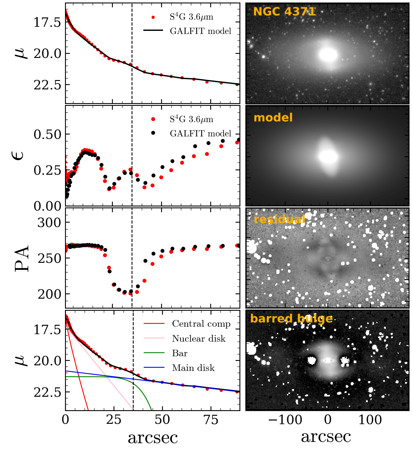
Figure 1: The photometric analysis of the S⁴G image and the GALFIT best-fitting model. The left column from top to bottom shows: 1D surface brightness profile, ellipticity, and position angle along the major axis of the S⁴G image (red) and GALFIT model (black). The last panel on the left column represents each component’s 1D surface brightness profile in the GALFIT best-fitting model (central compact source, nuclear disk, bar, and main disk). Right column from top to bottom: 2D surface brightness distribution of the NGC 4371 S⁴G image, GALFIT best-fitting model, the residual, and the bar extracted by subtracting the nuclear and main disks from the original image. The black dashed line indicates the projected bar radius $R_{\rm bar}^{{}^{\prime}}\sim 35$ arcsec. The image is flipped to align with the orientation of the kinematic map.

Fitting MGEs to the disk and bar:

we fit MGEs to the (nuclear+main) disk and the bar separately. Note that we use the residual bar, which allows us to capture the triaxiality better than the fitted elliptical bulge. We obtain parameters $(L_{j},q^{\prime}_{j},\sigma^{\prime}_{j},\Delta\psi_{j}^{\prime})$ of the 2D Gaussians from the fitting, where $L_{j}$ is the total luminosity, $q_{j}^{\prime}$ is the projected flattening, and $\sigma_{j}^{\prime}$ is the scale length along the projected major axis of each Gaussian component $j=1\dots N$. $\Delta\psi_{j}^{\prime}$ is the isophotal twist of each Gaussian. The MGE fitting parameters of the bar (Gaussians with $\Delta\psi_{j}^{\prime}\neq 0$) and the disk (Gaussians with $\Delta\psi_{j}^{\prime}=0$) are presented in Table 2.

Deprojection:

The orientation of a projected system is defined by three viewing angles $(\theta,\varphi,\psi)$, $\theta$ and $\varphi$ indicate the orientation of the line-of-sight with respect to the principal axes of the object. $\psi$ is the position angle which indicates the rotation of the object around the line of sight in the sky plane (see Fig. 2 in de Zeeuw & Franx (1989)). The intrinsic parameters describing a 3D Gaussian component $(\sigma_{j},p_{j},q_{j})$ can be derived analytically using a set of viewing angles $(\theta,\varphi,\psi)$ and parameters measured for the 2D Gaussians (see Eqs. (7-9) in VdB08). For a rigid body comprised of multiple Gaussian components, all Gaussians are fixed to have the same viewing angles, the allowed orientations are thus the intersection of allowed viewing angles $(\theta,\varphi,\psi)$ of all the Gaussians.

We deproject the disk and the bar separately. Thus, we have three viewing angles $(\theta_{\rm disk},\varphi_{\rm disk},\psi_{\rm disk})$ for the disk and three viewing angles $(\theta_{\rm bar},\varphi_{\rm bar},\psi_{\rm bar})$ for the bar.

The disk is considered as an axisymmetric oblate system with the major axis aligned with the $x^{\prime}$ axis of the image so that $\psi_{\mathrm{disk}}=90^{\circ}$, and all Gaussians have $\Delta\psi_{j}^{\prime}=0$, while $\varphi_{\rm disk}$ is irrelevant. The inclination angle of the disk $\theta_{\rm disk}$ is left as a free parameter, with its lower limit constrained by $\cos(\theta_{\rm disk})^{2}<q^{\prime 2}_{\rm min}$ where $q^{\prime}_{\rm min}$ indicate the flattest Gaussian of MGEs fitted to the disk.

The bar is triaxial, so its Gaussians can have different isophotal twists $\Delta\psi_{j}^{\prime}$. The twists of bar Gaussians are measured with respect to the disk’s major axis in the observational plane. We thus have $\Delta\psi_{j}^{\prime}=\psi_{j}^{\prime}-\psi_{\mathrm{disk}}$, and $\psi_{\rm bar}=\psi_{\rm disk}=90^{\circ}$, with the real information of the bar position angle included in $\Delta\psi_{j}^{\prime}$, which is directly measured from the image through the MGE fitting.

We combine the bar and disk together by enforcing the bar’s major axis to be aligned within the disk plane. This implies the inclination angle constraint to be $\theta_{\rm bar}=\theta_{\rm disk}$, and the angle $\varphi_{\rm bar}$ is left free. We thus have two viewing angles as free parameters in the triaxial bar de-projection: $\theta_{\rm disk}$ and $\varphi_{\rm bar}$, which will be just denoted as $\theta$ and $\varphi$ in what follows.

Once we infer the 3D luminosity density distribution, we multiply it with a constant stellar mass-to-light ratio $M_{*}/L$ to obtain the 3D stellar mass distribution. The stellar mass-to-light ratio $M_{*}/L$ is another free parameter in the mass model, which we assume to be constant for the whole galaxy. This is a good approximation given that the stellar age is quite homogeneous across the TIMER field Gadotti et al. (2015). For the triaxial bar model, we consider the gravitational potential is stationary in the rotating frame. Thus, the bar pattern speed $\Omega_{p}$ is left as another free parameter. In summary, we have five free so-called hyperparameters in the model: inclination $\theta$, bar azimuthal angle $\varphi$, stellar mass-to-light ratio $M_{*}/L$, DM virial mass $M_{\rm 200}$, and the bar pattern speed $\Omega_{p}$.

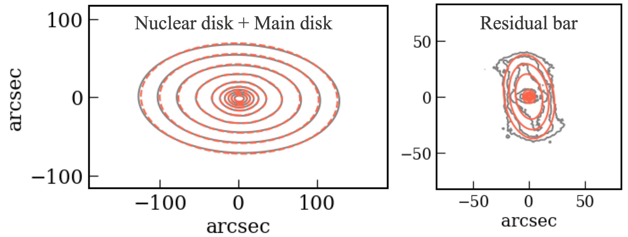
Figure 2: Left panel: The surface density contours of disk component (grey lines), overplotted with contours of the best-fitting MGE model (orange lines). Right panel: similarly for the bar, where the twist is allowed in the MGE model.

$j$	$L_{j}$ $(\mathrm{L_{\odot}pc^{-2}})$	$\sigma^{\prime}_{j}$ $(\mathrm{arcsec})$	$q^{\prime}_{j}$	$\Delta\psi_{j}^{\prime}$ $(^{\circ})$
$1$	3704.801	0.294	0.99	-59.0
$2$	8404.87	1.069	0.99	-59.0
$3$	2675.332	2.119	0.981	-66.0
$4$	439.306	18.296	0.58	-63.831
$5$	43.923	45.0	0.614	-59.611
$6$	3149.241	2.343	0.575	0.0
$7$	3343.404	5.112	0.58	0.0
$8$	2054.372	8.667	0.57	0.0
$9$	147.203	11.512	0.965	0.0
$10$	504.083	14.211	0.57	0.0
$11$	177.944	31.804	0.57	0.0
$12$	124.066	60.354	0.57	0.0
$13$	25.73	106.066	0.57	0.0

Table 2: The MGE fitting parameters of the bar (Gaussians with $\Delta\psi_{j}^{\prime}\neq 0$ ) and the disk (Gaussians with $\Delta\psi_{j}^{\prime}=0$ ).

3.2 Generating the Orbit Library

We sample the initial conditions of orbits using the properties of separable triaxial potential following VdB08. In this approach, the orbits are sampled from the three integrals of motion: energy, $E$, the second integral of motion, $I_{2}$, and the third integral of motion, $I_{3}$ Binney & Tremaine (2008). For the rotating triaxial bar model, we sample two sets of tube orbit libraries in $x-z$ plane, one with $v_{y}>0$ and the other with $v_{y}<0$ as discussed in Tahmasebzadeh et al. (2022). The number of starting points in each orbit library is $(E,I_{2},I_{3})=30\times 15\times 13$. For each starting point, we adopt orbit dithering of $3^{3}$ to form an orbit bundle.

4 Results

4.1 Best-fitting Models

We give each orbit bundle a weight, superpose them together, and try to fit the observational data. The data we used to constrain the model are stellar kinematic maps, the 2D surface brightness, and the 3D luminosity distribution deprojected from the MGE. The kinematic maps include the line-of-sight mean velocity $V$, velocity dispersion $\sigma$, the Gauss-Hermite (GH) coefficients $h_{3}$ and $h_{4}$. We fit all Gauss-Hermite coefficients of $h_{1}$, $h_{2}$, $h_{3}$, and $h_{4}$, see Tahmasebzadeh et al. (2022) for details. The orbit weights are solved by minimizing the $\chi^{2}$ between the data and model using a non-negative least squares (NNLS) implementation Lawson & Hanson (1974) following VdB08.

We have five free hyperparameters in the model: the stellar mass-to-light ratio $M_{*}/L$ at 3.6 $\mu$m band, inclination angle $\theta$, bar azimuthal angle $\varphi$, bar pattern speed $\Omega_{\rm p}$, and the DM virial mass $M_{200}/M_{*}$. We use an optimized grid iterative process to search for the best-fitting model. We start with initial guesses of the hyperparameters. We then walk two steps in each direction of the parameter grid by taking relatively large intervals of $0.2$, $6$, $2$, $2$, and $0.4$ for $M_{*}/L$, $\Omega_{\rm p}$, $\theta$, $\varphi$, and $\mathrm{log_{10}}(M_{200}/M_{*})$, respectively. Once the previous models are completed, we select models with $\chi^{2}-\chi^{2}_{\rm min}<f\times\sqrt{2n_{\rm GH}N_{\rm kin}}$ and start an iterative process to run new models around the selected models. The iterative process will stop when the minimum $\chi^{2}$ model is found and all models around are calculated. $n_{\rm GH}$ is the number of velocity maps which is $4$ as we use $V$, $\sigma$, $h_{3}$, and $h_{4}$. $N_{\rm kin}$ is the number of apertures in one kinematic map, which is $N_{\rm kin}=1442$ for TIMER data and $N_{\rm kin}=1048$ for ATLAS3D data. The factor of $f$ is chosen empirically depending on the data, so we use $f=100$ for modeling with TIMER data and $f=50$ for ATLAS3D data. At the end, we run the iterative searching process again with a larger factor of $f$ (e.g., $2\times f$) to avoid being trapped in the local minimum and ensure all models within $3\sigma$ confidence level are calculated.

In the classic statistic analysis for analytic models fitting to data, the $1\sigma$ confidence level is determined by $\Delta\chi^{2}=1$. However, it is unsuitable for our case where the model numerical noise dominates the $\chi^{2}$ (Lipka & Thomas, 2021). In Zhu et al. (2018b), $\Delta\chi^{2}\equiv\sqrt{2n_{\rm GH}N_{\rm kin}}$ is adopted as $1\sigma$ confidence level, which is consistent with the $\chi^{2}$ fluctuation caused by numerical noise of their models for CALIFA galaxies. Here, we calculate the $1\sigma$ confidence level in a similar approach using bootstrapping process. We perturb the kinematic data with its errors randomly and create $100$ new kinematic maps. Then we pick our best-fitting model with fixed potential and orbit library and re-fit with the $100$ perturbed data. The standard deviation of $\chi^{2}$ distribution obtained from these fittings is taken as the $\chi^{2}$ fluctuation caused by the numerical noise of the model. In this way, we found the $1\sigma$ confidence level for the models constrained by TIMER to be $\sim 0.5\times\sqrt{2n_{\rm GH}N_{\rm kin}}$ and for models constrained by ATLAS3D data to be $\sim 2\times\sqrt{2n_{\rm GH}N_{\rm kin}}$.

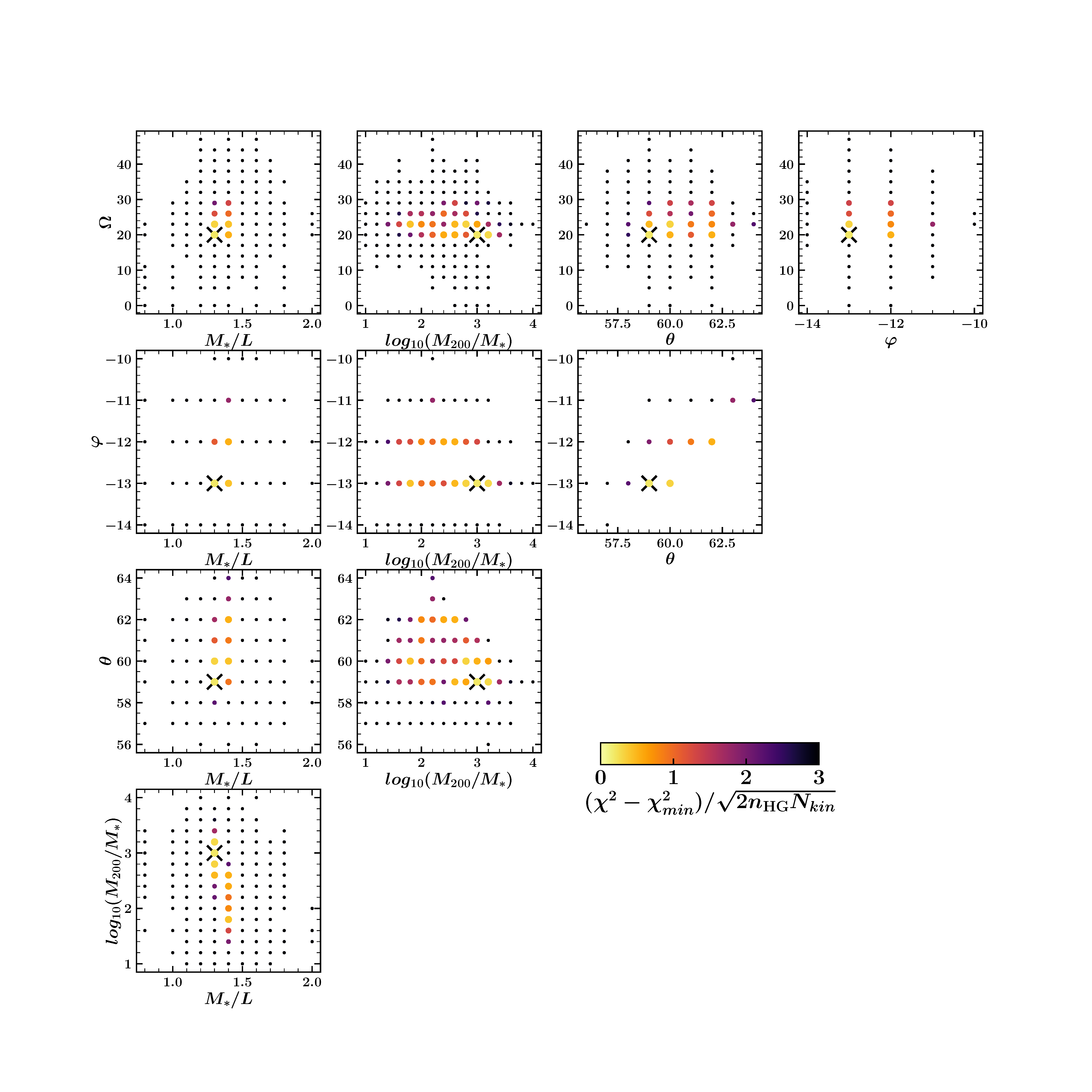
Figure 15: The parameter grid we explored for the bar model fitting using TIMER data. The five hyperparameters are stellar mass-to-light ratio $M_{*}/L_{3.6um}$ in unit of $M_{\odot}/L_{\odot}$, dark matter halo mass $\log M_{200}/M_{*}$, the inclination angle of the disk $\theta$, the bar angle with respect to the major axis of the disk $\varphi$, and the pattern speed $\Omega_{\rm p}$ in units of $\mathrm{km\hskip 1.13791pts^{-1}\hskip 1.13791ptkpc^{-1}}$. Each point is one model color-coded according to their $\chi^{2}$ values shown in the color bar. The points with $(\chi^{2}-\chi^{2}_{min})/\sqrt{2n_{\rm GH}N_{\rm kin}}<1$ indicate models within $1\sigma$ confidence level. The black crosses indicate the best-fitting model.

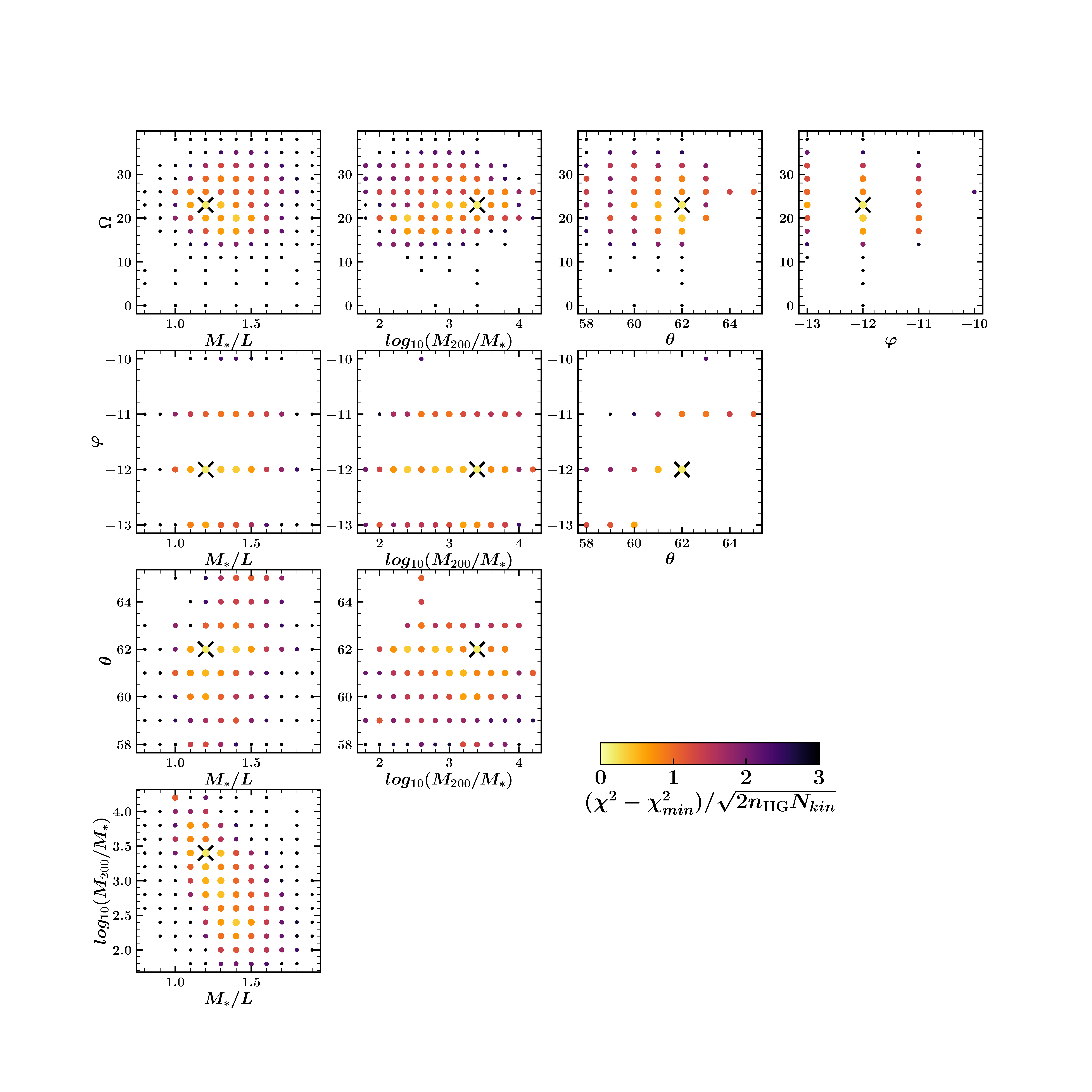
Figure 16: Same as Fig. 15 but for the bar model fitting using ATLAS3D data

We take all the models within the $1\sigma$ confidence level, and calculate the mean and standard deviation of each parameter within these models, which we take as the best-fitting parameter and its $1\sigma$ error. From the models constrained by TIMER, we thus obtained $\theta=60\pm 2^{\circ}$, $\varphi=-12\pm 1^{\circ}$, $\Omega_{\rm p}=23.6\pm 2.8\hskip 2.27626pt\mathrm{km\hskip 1.13791pts^{-1}\hskip 1.13791ptkpc^{-1}}$, $M_{*}/L_{3.6\mu m}=1.35\pm 0.05$ $M_{\odot}/L_{\odot,3.6\mu m}$, and DM virial mass $\log_{10}(M_{200}/M_{*})=2.4\pm 0.5$. From the models constrained by ATLAS3D, we obtain $\theta=60\pm 2^{\circ}$, $\varphi=-12\pm 1^{\circ}$, $\Omega_{\rm p}=22.4\pm 3.5\hskip 2.27626pt\mathrm{km\hskip 1.13791pts^{-1}\hskip 1.13791ptkpc^{-1}}$, $M_{*}/L_{3.6\mu m}=1.27\pm 0.11$ $M_{\odot}/L_{\odot,3.6\mu m}$, and DM virial mass $\log_{10}(M_{200}/M_{*})=3.0\pm 0.6$. The parameters obtained from the sets of models are generally consistent with each other. The model using ATLAS3D data has larger uncertainty due to a smaller spatial coverage than MUSE data. The parameters grid of all models are included in Appendix Fig. 15 and Fig. 16. In $3.6$ $\mu$m band, by assuming Chabrier initial mass function (IMF), the stellar population synthesis gives an average of $\Upsilon_{3.6\mu m,*}^{\mathrm{Chab}}\sim 0.6$, with uncertainty of 0.1 dex Meidt et al. (2014), which is lower than the dynamical stellar mass-to-light ratio $\Upsilon_{3.6\mu m,*}^{\mathrm{dyn}}\sim 1.3$ we obtained. If we scale it to a Salpeter IMF multiplied by a factor of 1.8, then $\Upsilon_{3.6\mu m,*}^{\mathrm{Slap}}\sim 1.1$ is consistent with our dynamical results within $1\sigma$ uncertainty.

We present the best-fitting models of NGC 4371 in Fig. 3. Columns from left to right show the 2D surface density, LOS velocity, velocity dispersion, $h_{3}$, and $h_{4}$. The first to third rows represent TIMER data covering $\sim 35$ arcsec, the best-fit Schwarzschild bar model, and the residuals, computed as the difference between the TIMER data and the model, divided by the uncertainties of TIMER data in each bin. The fourth to sixth rows show the ATLAS3D data within $\sim 20$ arcsec, the best-fit Schwarzschild bar model, and the residuals. All panels are overplotted with gray contours indicating the surface brightness of the NGC 4371. Our models reproduce all the key kinematic features well, from the nuclear disk to the outer bar regions. The fitting to the kinematic maps is improved compared to a nearly axisymmetric model not explicitly including the bar. In appendix A, we discuss how an axisymmetric model can still fit the data, but the internal properties of the best-fit model are significantly biased (see Fig. 13).

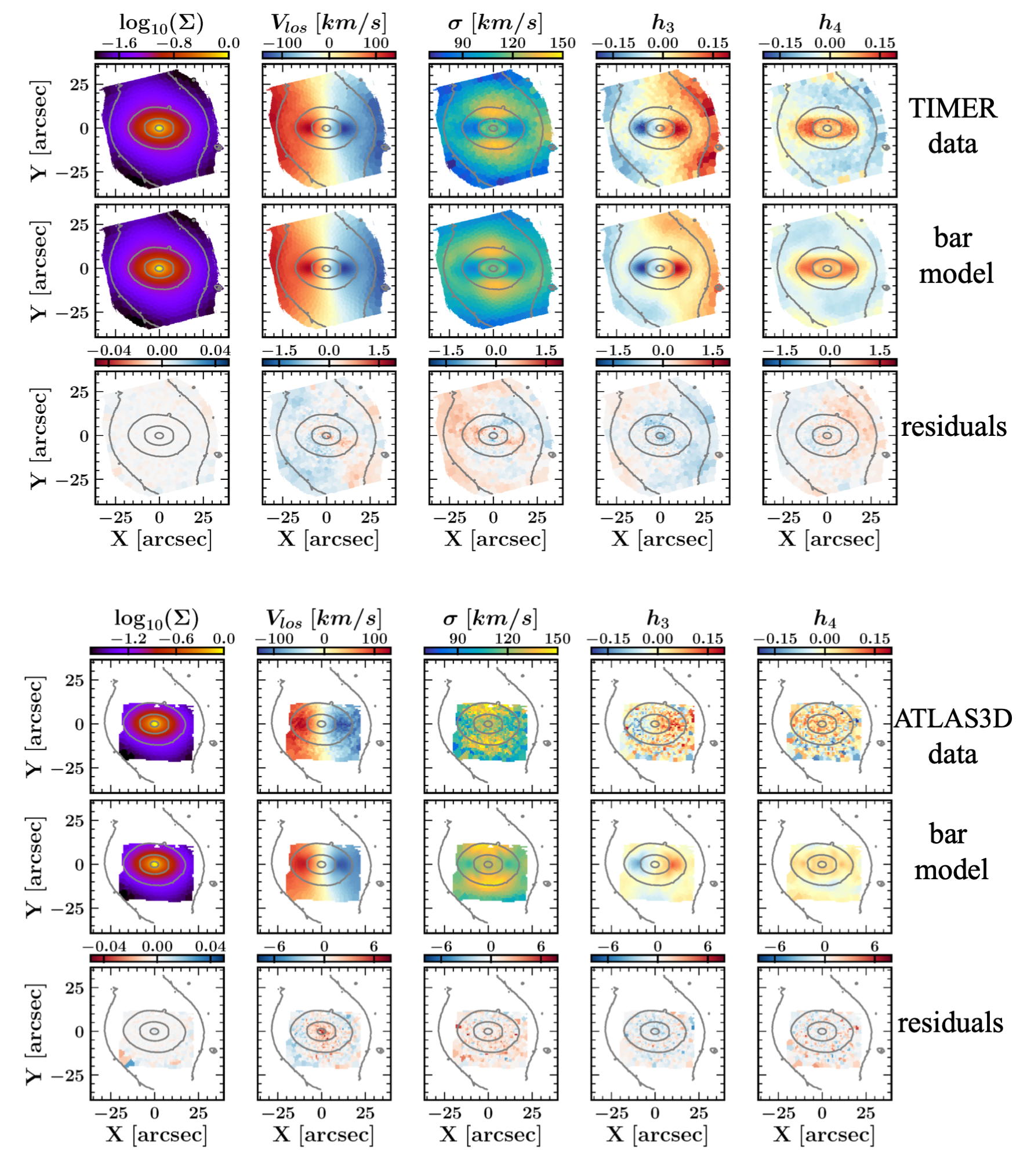
Figure 3: The best-fitting models of NGC 4371, to the data from TIMER (top panel) and ATLAS3D (the bottom), respectively. In each panel, columns from left to right represent the 2D surface density, velocity, velocity dispersion, $h_{3}$, and $h_{4}$, rows from top to bottom are the observational data, the best-fit Schwarzschild barred model, and the residuals. The overplotted gray contours are the surface brightness of the NGC 4371. The TIMER data covers the regions with $r\lesssim 35$ arcsec, while ATLAS3d covers only the inner regions with $r\lesssim 25$ arcsec, the data are well matched in both sets of the models.

4.2 The Bar Pattern Speed and Rotation Parameter

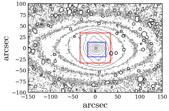
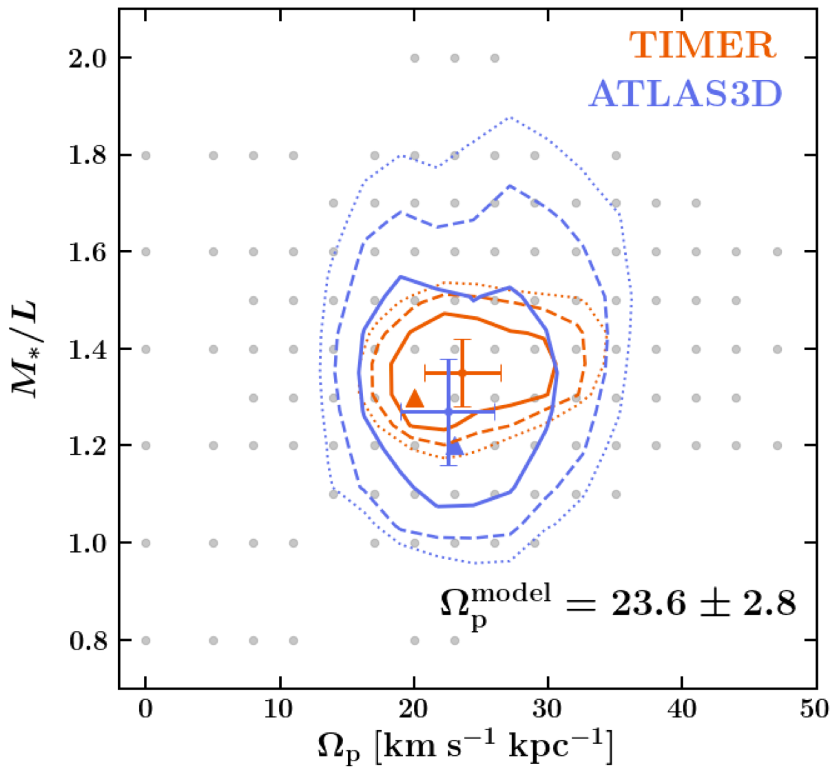
Figure 4: The bar pattern speed obtained from the two sets of models constrained by TIMER and ATLAS3D separately. Top panel: the spatial coverage of TIMER (red) and ATLAS3D (blue) data comparing to the whole galaxy, with contours showing the $3.6$ $\mu$m S⁴G image. Bottom panel: the model parameter grid bar pattern speed $\Omega_{\rm p}$ versus the stellar mass-to-light ratio $M_{*}/L_{3.6um}$. The contours indicate the $1\sigma$ (solid line), $2\sigma$ (dashed line), and $3\sigma$ (dotted line) uncertainties for the best-fitting models using TIMER (red) and ATLAS3D (blue). The small dot with error bars indicates the mean and $1\sigma$ uncertainty obtained from the models within the $1\sigma$ confidence level. The triangles indicate the best-fitting model for each data set. The pattern speed obtained from the two sets of models are well consistent with each other, with smaller uncertainty from the model constrained by TIMER.

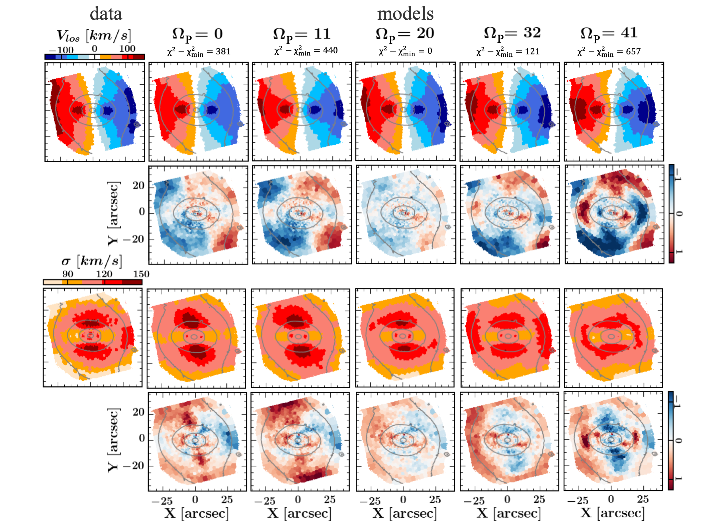
Figure 5: The kinematic maps predicted by models with different pattern speeds. The first column shows velocity (top) and velocity dispersion (bottom) from TIMER data, the following columns from left to right are the model predictions with pattern speed of $\Omega_{\rm p}=0,11,20,32,41$ $\rm kms^{-1}kpc^{-1}$ in which $\Omega_{\rm p}=20$ $\rm kms^{-1}kpc^{-1}$ is the best-fitting model. All other parameters kept the same as the best-fitting model. The second and fourth rows represent the corresponding residuals. The residuals of both the velocity and velocity dispersion maps become significantly larger with the pattern speed deviating from the best-fitting model ($\Omega_{\rm p}=20$ $\rm kms^{-1}kpc^{-1}$).

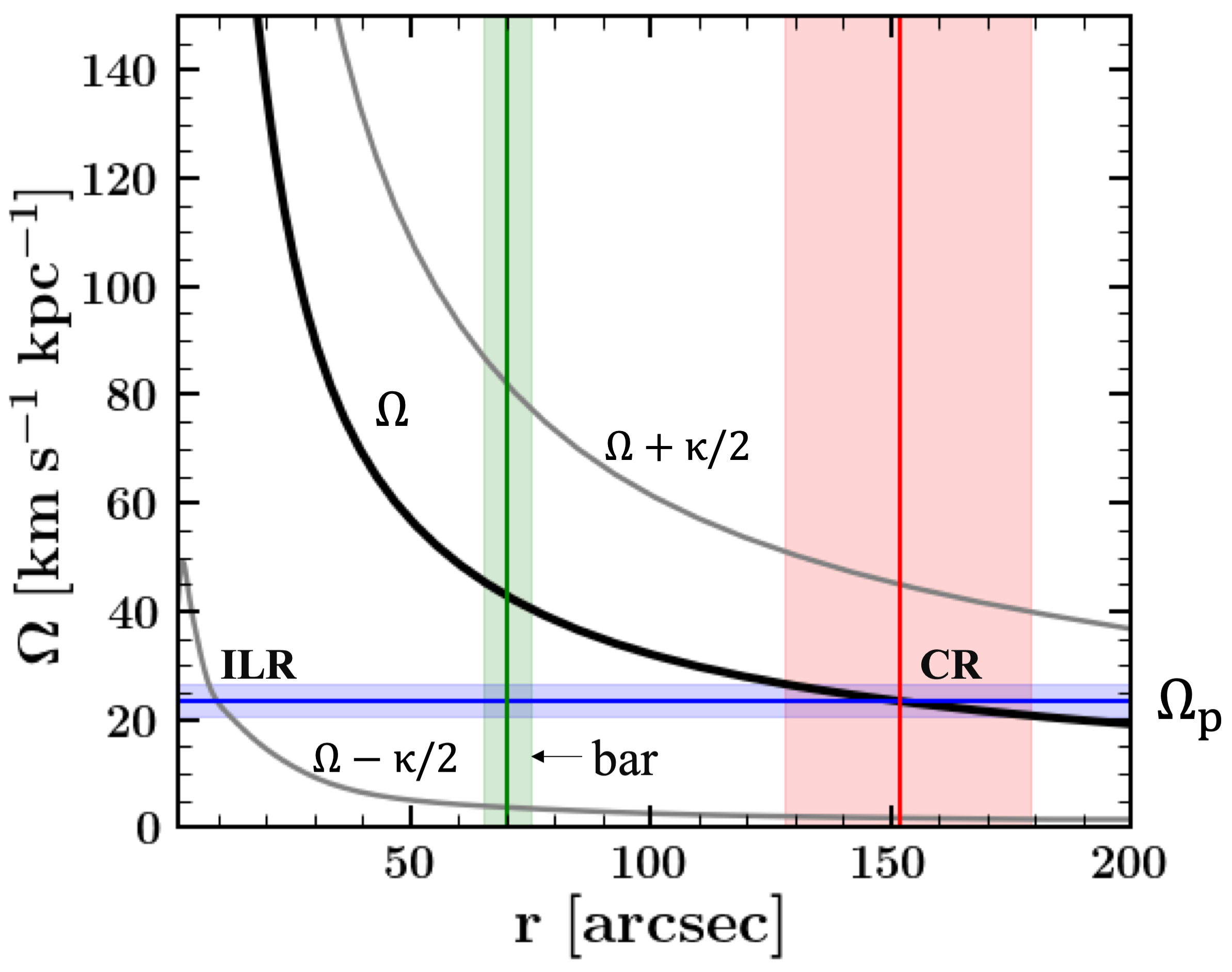
Figure 6: The resonance radii from our best-fitting bar model. The black curve indicates the local angular frequency $\Omega$. The gray curves show $\Omega-\kappa/2$ and $\Omega+\kappa/2$ where $\kappa$ is the local radial epicyclic frequency. The horizontal blue line with shaded regions represents the measured pattern speed and its $1\sigma$ uncertainty obtained from our models constrained by TIMER. The vertical green line indicates the bar radius $R_{\rm bar}\sim 69$ arcsec measured by photometric decomposition, with the shaded regions indicating the lower/upper limit of the bar radius from Erwin et al. (2008). The vertical red line with shaded regions indicates the location of corotation resonance (CR: $\Omega=\Omega_{p}$) at $\sim 153$ arcsec and the $1\sigma$ uncertainty.

4.2.1 The bar pattern speed

Neither the TIMER nor the ATLAS3D data covers the disk-dominated regions of NGC 4371, as shown in the upper panel of Fig. 4, which makes it hard to determine the bar pattern speed with the TW method. However, we can provide good constraints on the pattern speed with the limited data coverage through our model. In the bottom panel of Fig. 4, we illustrate the parameter space of $\Omega_{\rm p}$ verse $M_{*}/L$ constrained by TIMER (red) and ATLAS3D (blue) data. The solid, dashed, and dotted lines indicate the confidence level of $1\sigma$, $2\sigma$, and $3\sigma$ regions, respectively. We find the bar pattern speed of $\Omega_{\rm p}=23.6\pm 2.8\hskip 2.27626pt\mathrm{km\hskip 1.13791pts^{-1}\hskip 1.13791ptkpc^{-1}}$ and $\Omega_{\rm p}=22.4\pm 3.5\hskip 2.27626pt\mathrm{km\hskip 1.13791pts^{-1}\hskip 1.13791ptkpc^{-1}}$ from the models constrained by TIMER and ATLAS3D data, respectively.

To further understand how the pattern speed is constrained by the kinematic data, in Fig. 5, we compare the kinematic maps predicted by models with different pattern speeds. The first column shows velocity (top) and velocity dispersion (bottom) for the TIMER data. The models with pattern speed of $\Omega_{\rm p}=0,11,20,32,41$ $\rm kms^{-1}kpc^{-1}$ are presented by columns from left to right in which $\Omega_{\rm p}=20$ $\rm kms^{-1}kpc^{-1}$ is the best-fitting model. All other parameters are kept the same as the best-fitting model. The second and the fourth rows represent the residuals, computed as the difference between the TIMER data and the model, divided by the uncertainties of TIMER data at each bin. As shown in residual maps, by getting far from $\Omega_{\rm p}=20$ $\rm kms^{-1}kpc^{-1}$, the value of $\chi^{2}$ increases significantly. With smaller $\Omega_{\rm p}$ than the best-fitting value, the regular rotation predicted by the model is too small in the outer bar regions, and the dispersion in the two high-dispersion lobes becomes too large. On the other side, the model predicted regular rotation in the outer bar regions gets too strong, and the two high-dispersion lobes disappear. Both velocity and dispersion maps play important roles in constraining the pattern speed in our Schwarzschild model.

Besides having an extended data coverage, the TW method demands optimal orientation of the disk and the bar for precise measurements of pattern speed. As discussed in Zou et al. (2019), a disk nearly face-on/edge-on or a bar nearly parallel/perpendicular to the disk major axis could lead to a wrong measurement of the pattern speed. The bar in NGC4371 is nearly perpendicular to the main axis of the disk. We tried to apply the TW method to NGC 4371 and yielded a pattern speed of approximately $\sim 220$ $\rm km\,s^{-1}kpc^{-1}$, which is evidently erroneous.

4.2.2 The dimensionless bar rotation parameter $\mathcal{R}$

We first compute the local angular frequancy $\Omega$ and the epicyclic frequency $\kappa$ using the best-fitting model potential $\Phi$, following Binney & Tremaine (2008)

$$\Omega=\sqrt{\frac{1}{r}\frac{\mathrm{d}\Phi}{\mathrm{~{}d}r}}$$ (1)

$$\kappa=2\Omega\sqrt{\left(1+\frac{r}{2\Omega}\frac{\mathrm{~{}d}\Omega}{\mathrm{~{}d}r}\right)},$$ (2)

and we show the frequencies of $\Omega$ (black curve) and $\Omega\pm\kappa/2$ (gray curves) versus radius in Fig.6. Assuming the bar is rotating as a solid body with the angular velocity of $\Omega_{p}$, we can thus derive resonances with the rotating matter in the disk. There are three important resonances in a barred galaxy: the corotation resonance (CR: $\Omega=\Omega_{p}$), Inner Lindblad resonance (ILR: $\Omega-\kappa/2=\Omega_{p}$), and Outer Lindblad resonance (OLR: $\Omega+\kappa/2=\Omega_{p}$). The bar co-rotation radius $R_{\rm cor}$ is determined as the location of corotation resonance where $\Omega(R_{\rm cor})=\Omega_{\rm p}^{\rm model}$. Then, we derive the bar rotation rate using $\mathcal{R}\equiv R_{\rm cor}/R_{\rm bar}$.

We consider the uncertainties on bar radius and bar pattern speed as the major source of uncertainty on the bar rotation rate $\mathcal{R}$. For the bar radius, we measured $R_{\rm bar}=69$ arcsec ($\sim 5.7$ $\rm kpc$) from the photometry and considered the upper and lower limits of 64 and 75 arcsec (Erwin et al., 2008). We obtained $\Omega_{\rm p}=23.6\pm 2.8$ $\rm kms^{-1}kpc^{-1}$ from the model constrained by TIMER data, the corresponding bar co-rotation radius is $R_{\rm cor}=153\pm 25$ arcsec ($\sim 12.5$ $\rm kpc$). Considering the $1\sigma$ lower/upper limit of $R_{\rm bar}$ and $R_{\rm cor}$, we obtain $\mathcal{R}=2.2\pm 0.4$. A barred galaxy can be classified as a fast (if $1<\mathcal{R}<1.4$) or a slow bar (if $\mathcal{R}>1.4$) Debattista & Sellwood (2000). Therefore, we conclude that NGC 4371 is a slow bar, even considering the lower limits of $\mathcal{R}=1.8$. Numerical simulations show that once the bar is formed, it may experience a strong drag due to the dynamical friction of the DM halo. Thus the bars may slow down on time scales depending on the DM content in the disk region Debattista & Sellwood (1998b, 2000); Athanassoula & Misiriotis (2002); Fragkoudi et al. (2021).

4.3 Intrinsic Structure and Mass Profile

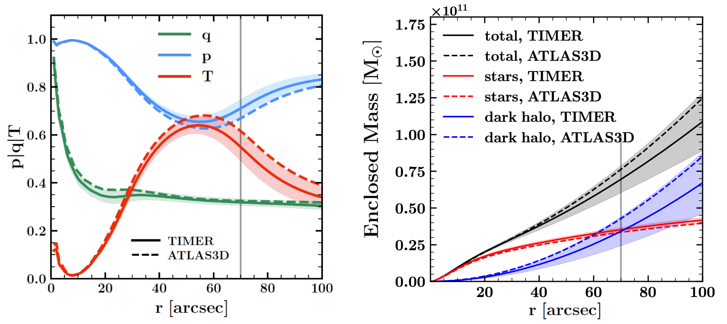
Figure 7: Left panel: the axial ratios $q=c/a$ (green), $p=b/a$ (blue), and triaxial parameter $T=(1-p^{2})/(1-q^{2})$ (red) as a function of intrinsic radius, for the best-fitting bar models constrained by TIMER (solid line) and ATLAS3D (dashed line). Right panel: enclosed mass profiles of the best-fitting bar models constrained by TIMER (solid line) and ATLAS3D (dashed line). The red, blue, and black curves represent the stellar mass, dark matter mass, and total mass, respectively. The shaded regions indicate the $1\sigma$ uncertainty from the set of models constrained by TIMER. The vertical gray line indicates the bar length $R_{\rm bar}\sim 70$ arcsec.

We calculate the intrinsic axis ratios $p=b/a$, $q=c/a$, and triaxiality $T=\frac{1-p^{2}}{1-q^{2}}$ as a function of radius for the best-fitting models, the variation among the models within $1\sigma$ confidence level is taken as the $1\sigma$ uncertainty. The results from the model constrained by TIMER and ATLAS3D are consistent with each other. As shown in Fig.7, the galaxy is round with large $q$ at the inner regions due to the spherical compact Sérsic component; $q$ sharply drops at $r\sim 10$ arcsec and then changes smoothly to the main disk with $q=0.31$. The maximum triaxiality happens at the $\sim 77\%$ of the bar radius, which is roughly the transition point from the bar to the disk.

We show the enclosed mass profiles of NGC 4371 in the right panel of Fig. 7. The black, red, and blue curves represent the total enclosed mass, stellar mass, and DM mass profiles, respectively. The shaded regions represent the $1\sigma$ uncertainty from the models with TIMER. The total mass profiles are well constrained with $1\sigma$ uncertainties of $~{}10$ percent within data coverage of $35$ arcsec. The results from the models constrained by ATLAS3D are consistent, have relatively large uncertainties in the outer regions with smaller data coverage. NGC 4371 has a high dark matter fraction of $M_{\rm DM}/M_{\rm total}\sim 0.51\pm 0.06$ within the bar region. It is similar to the dark matter fraction ($\sim 0.53\pm 0.02$) of NGC 4277 inside the bar regions, which is the first observed slow bar reported that coupled the bar rotation parameter to the dark matter fraction Buttitta et al. (2023).

4.4 Structure Decomposition and Their Internal Properties

4.4.1 The orbit distribution in $\lambda_{z}$ verse. $r$

We first characterize the stellar orbits by two parameters following Zhu et al. (2018b): the circularity $\lambda_{z}$ defined as the angular momentum $L_{z}$ (recorded in an inertial frame) normalized by the maximum allowed by a circular orbit with the same binding energy and the radius $r$ taken as the average of particles along an orbit stored with equal time steps in the Schwartzchild model.

We show the stellar orbit distribution of the best-fitting model constrained by TIMER in the space of circularity $\lambda_{z}$ versus radius $r$ in the left panel of Fig. 8. The vertical dotted line indicates the bar radius, which is within the kinematic coverage of TIMER data. The highly circular orbits ($\lambda_{z}\sim 1$) distributed in the inner and outer regions make up the nuclear and main disks. The non-circular orbits could construct a classical bulge, and could also be part of the bar. The bar orbits overlap with the orbits of the classical bulge in the phase-space of $\lambda_{z}$ versus $r$.

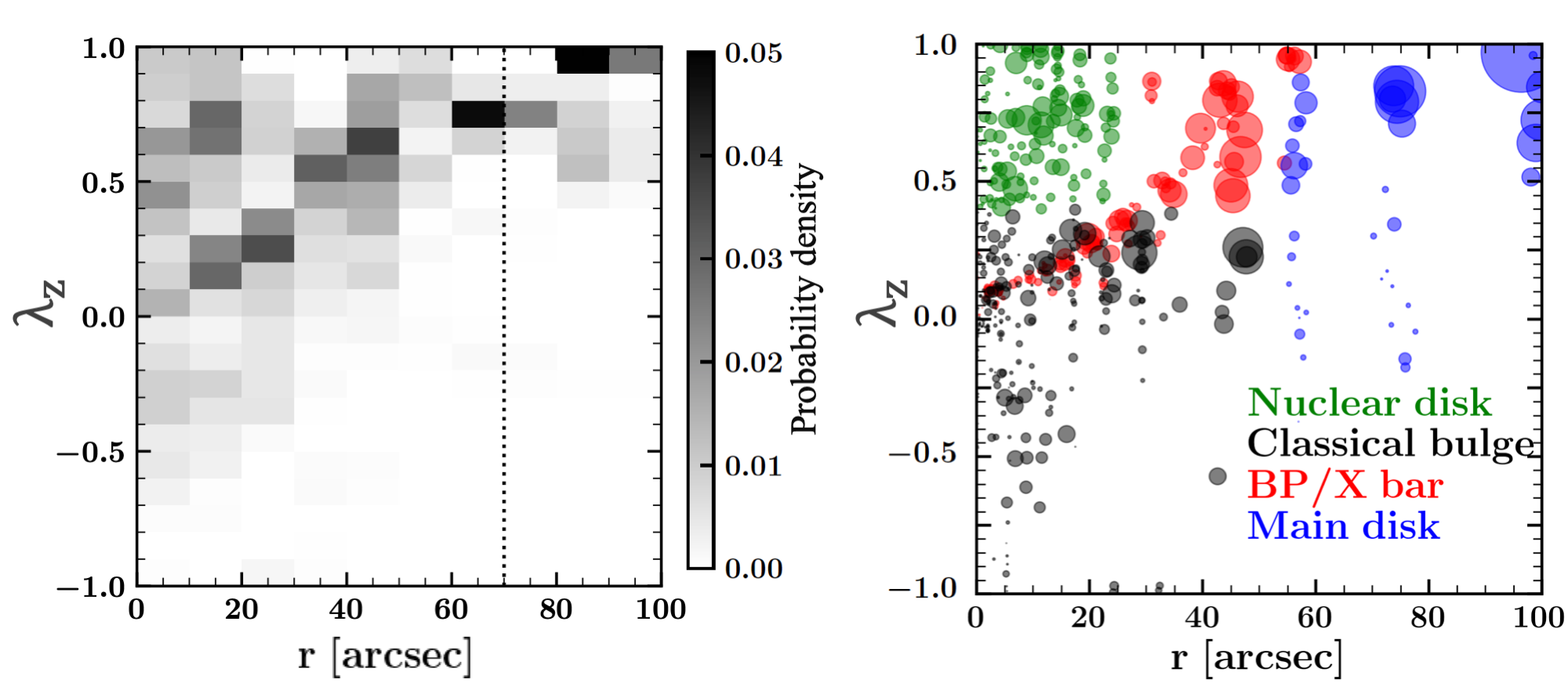
Figure 8: The stellar orbit distribution of the best-fitting model constrained by TIMER data. Left panel: the probability density distribution of orbits in the space of circularity $\lambda_{z}$ vs. time-averaged radius $r$. Darker color indicates a higher probability density as indicated by the colorbar. The vertical dotted lines indicate the bar radius and kinematics data extent of TIMER. Right panel: the location of orbits making up different structures: BP/X bulge (red), classical bulge (black), nuclear disk (green), and main disk (blue). The larger symbol size corresponds to orbits with higher weights from the minimum value of $10^{-7}$ to a maximum of $10^{-1}$ (the total weight of all orbits is $=1$).

4.4.2 Orbital decomposition

To further identify the orbits making up the bar, we analyze the non-zero weighted orbits of the best-fitting model following Tahmasebzadeh et al. (2022) using the NAFF software . We compute the orbital frequencies and classify the orbits into different types Valluri & Merritt (1998); Valluri et al. (2016). This orbit classification helps us identify different structures, especially barred ones.

We divide all orbits into four groups (1) BP/X bar: including $x_{1}$, banana ($1:2$ resonance), periodic and non-periodic $z$-tube orbits which are within the bar and elongated along the bar. These orbits are prograde short-axis tube orbits elongated along the bar and display an X-shaped structure in edge-on and face-on projected surface densities, consistent with previous studies Portail et al. (2015); Abbott et al. (2017); Fragkoudi et al. (2017); Parul et al. (2020) and our analysis of the orbital structures in a few simulations with BP/X bulges (Tahmasebzadeh et al. 2023, in preparation); (2) Classical bulge: non-circular orbits with $\lambda_{z}<0.4$. The classical bulge orbits are mainly nonperiodic box orbits that generate a hot, dispersion-dominated, and round structure in the face-on and edge-on images. (3) Nuclear disk: a rotation-dominated structure perpendicular to the bar constructed by highly circular orbits with $\lambda_{z}>0.4$ in the inner regions; (4) Main disk: all orbits with apocenter radii larger than the bar radius ($R_{\rm apo}>R_{\rm bar}$). It is dominated by highly circular orbits. Note that the orbits in the main disk extend well beyond the range of the available kinematic data, so they are constrained solely by the luminosity distribution of the galaxy. We show the location of the four structures in the phase space of $\lambda_{z}$ vs. $r$ in the right panel of Fig. 8, the disk orbits are separated from classical bulge by $\lambda_{z}$, the nuclear and main disks are separated by the bar, while the bar orbits in the inner regions partly overlap with orbits constructing the classical bulge.

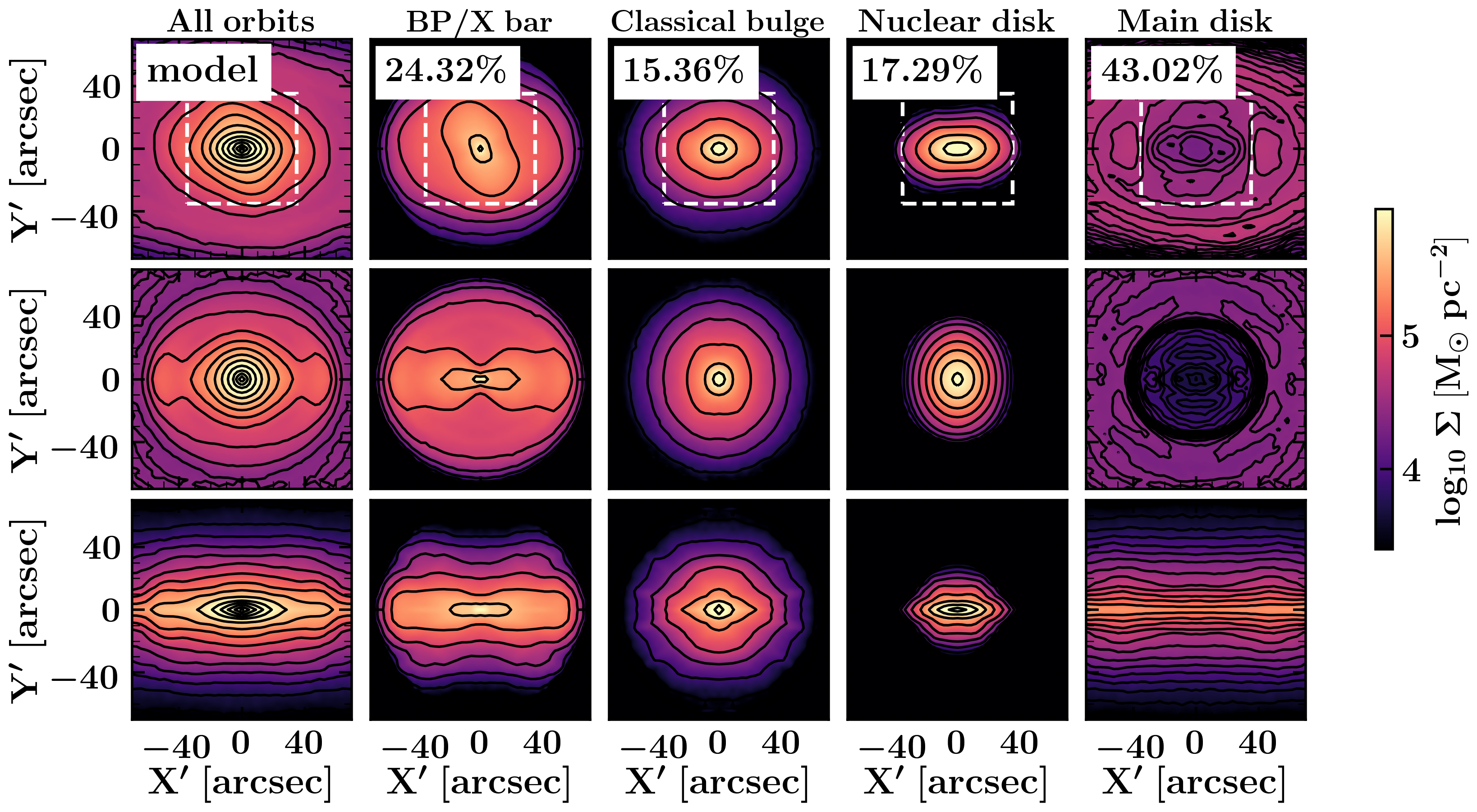
Figure 9: The surface density of different orbital structures decomposed from our best-fitting model constrained by TIMER data. The rows from top to bottom are projections with the observed galaxy orientation (top), face-on (middle), and edge-on (bottom) views. Columns from left to right show the reconstructed surface densities of the whole galaxy, the BP/X-shaped bar, the classical bulge, the nuclear disk, and the extended main disk, respectively. The white dashed squares in the first row indicate the data coverage. The luminosity fraction of each structure within the data coverage is tagged in the top row (in percent).

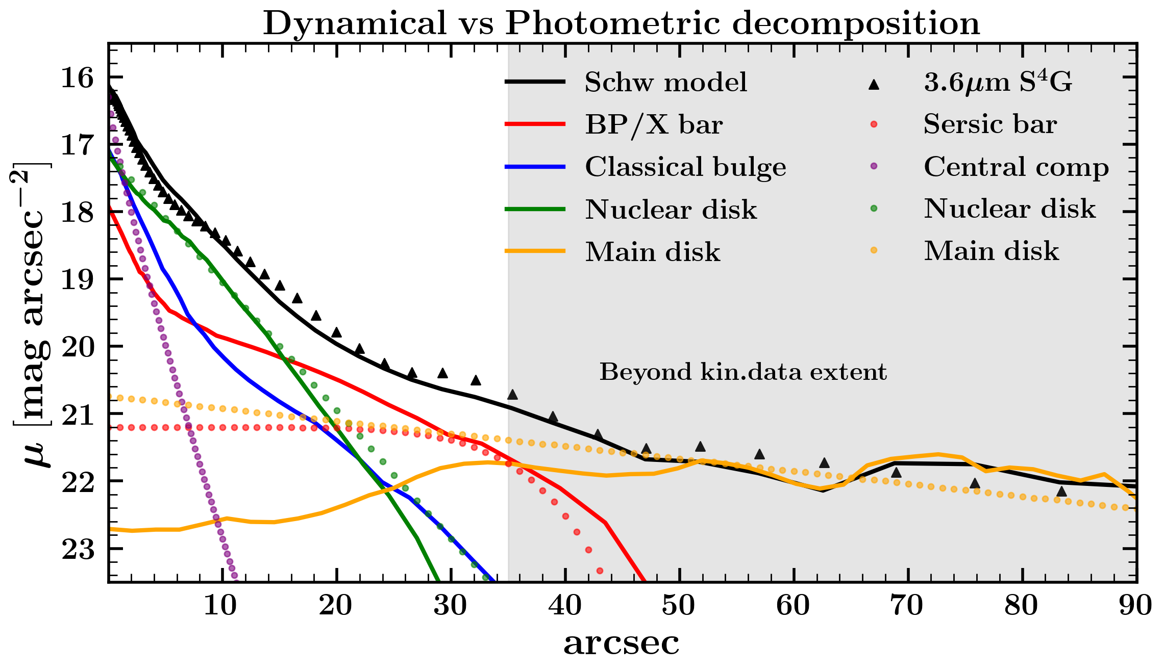
Figure 10: Comparsion of dynamical structure decompostion with photometric decomposition. Solid lines are the 1D surface brightness profiles along the major axis for different orbital structures decomposed from our best-fitting model constrained by TIMER data. The dotted lines indicate those of the structures from the GALFIT decomposition of S⁴G image. The shaded gray area represents regions beyond the kinematic data coverage.

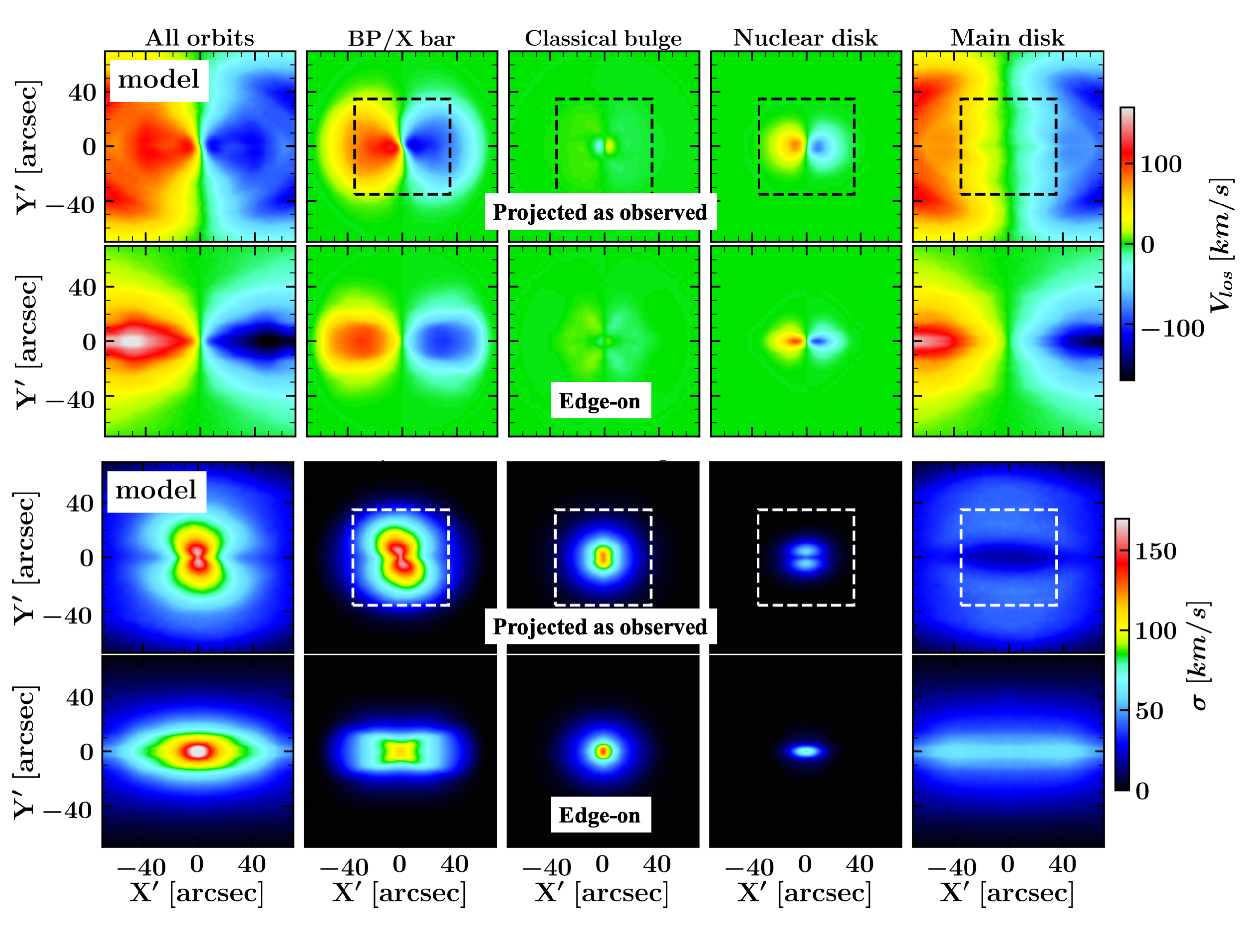
Figure 11: The kinematic maps of different structures decomposed from our best-fitting model. The first and the second rows show the velocity maps of the galaxy projected as observed and edge-on views. The third and fourth rows show the velocity dispersion maps of the galaxy projected as observed and edge-on views. Columns from left to right show the reconstructed kinematic maps of the whole galaxy, the BP/X-shaped bar, the classical bulge, the nuclear disk, and the extended main disk, respectively. The white dashed squares in the first column indicate the data coverage.

4.4.3 Morphology and kinematics of the four structure

We reconstruct the 3D density distribution and kinematics of each structure by summing the particles sampled from the orbits in each group. In Fig. 9, we illustrate the surface densities of different structures by projecting them with the orientation as the galaxy was observed, in face-on and edge-on views, respectively. Columns from left to right are surface densities of BP/X bar, classical bulge, nuclear disk, and disk orbits, respectively. The white square indicates the spatial coverage of TIMER data.

Our results confirm that NGC 4371 has a BP/X bulge that co-exists with a classical bulge contributing nearly similar fractions to the total surface density. The second and third rows in Fig. 9 represent this structure in different orientations. The BP/X bulge is not directly visible from the 2D image of this galaxy, and our model does not have an X-shaped structure in the input 3D density distribution, where the bar is mostly prolate, deprojected from the 2D image. Although an X-shaped structure is thus not explicitly included in the gravitational potential, the model can still support orbits constructing the X-shaped structure, and the kinematic data constraints pick up the orbits contributed to the BP/X structure (see Fig. 5, Fig. 11). This is a key point of our model as we discussed in Tahmasebzadeh et al. (2021, 2022).

We then quantify the luminosity fraction of different structural components in the best-fitting model. The contributions of the four components to the total luminosity of the galaxy are $24.32\%$ BP/X bar, $15.36\%$ classical bulge, $17.29\%$ nuclear disk, and $43.02\%$ main disk. When considering only the region within the data coverage, these fractions change to $34.92\%$ BP/X bar, $25.69\%$ classical bulge, $30.23\%$ nuclear disk, and $9.16\%$ main disk, respectively. Note that we have flexibility in seperating the classic bulge and inner disk, if we choose a different of $0.1$ in the $\lambda_{z}$ cut-off, the classical bulge and nuclear disk fractions will change by $2\%$ to $5\%$.

In our model, the radially end-to-end separation of the X-shaped structure is approximately half of the bar length. This proportion is consistent with what is measured for the Galactic bar Li & Shen (2012); Portail et al. (2017). A barlens structure was reported in NGC 4371 Buta et al. (2015); however, we show that it is actually a nuclear disk in the central regions in agreement with Gadotti et al. (2015), and it does not contribute to the BP/X structure. Erwin et al. (2015) employed 1D photometric decomposition to estimate the stellar mass ratio of the classical bulge to the total galaxy, finding it to be less than $10\%$ for NGC 4371, which is lower than the fraction of the classic bulge we found dynamically.

To understand the different results from the dynamical structure decomposition and the photometric decomposition, we show a direct comparison in Fig. 10. One main discrepancy could arise from the assumption of an exponential disk in photometric decomposition, while a dynamically defined disk is not necessarily exponential in all galaxies Zhu et al. (2018b); Breda et al. (2020); Ding et al. (2023). In our case, the main disk exhibits a luminosity in the inner regions much lower than the inward extrapolation of an exponential profile from the outer regions. Although the nuclear disk closely approximates an exponential distribution, it is consistent with the results from photometric decomposition.

In the following, we will investigate the kinematic properties associated with these structures to validate the accuracy of our decomposition. We show the LOS velocity (the first and second rows) and velocity dispersion (the third and fourth rows) of each component in Fig.11, by projecting them in the viewing angles as the galaxy was observed and edge-on, respectively. In the maps projected as observed, the inner region of the BP/X bar shows the strongest regular rotation, which is caused by stellar motion through an X-like (or a $\infty$-like) path along the bar and moving inward/outward from the disk plane. The total velocity dispersion map displays two high-dispersion lobes in the vertical direction. This enhancement is caused by a combination of the BP/X structure and the classical bulge. In the BX/P bar, velocity dispersion increases in two wings of the X-shaped structure. In the map projected edge-on, the BP/X bar has moderate rotation, and it creates relatively high dispersion in an X-shaped area. The classical bulge, characterized by its dynamically hot nature, exhibits no apparent rotation and contributes to an enhanced velocity dispersion at the center. A weak counter-rotationg motion in the very central region of classical bulge is due to orbits with $\lambda_{z}<0$. On the contrary, both the nuclear and main disks demonstrate strong regular rotation coupled with low dispersion.

5 Conclusions

We apply the triaxial Schwarzschild barred model presented in Tahmasebzadeh et al. (2022) to an S0 barred galaxy NGC 4371. The gravitational potential is adopted as the combination of a 3D stellar luminosity density multiplied by a constant stellar mass-to-light ratio, a spherical dark matter halo, and a fixed black hole. We use the 3D stellar luminosity density deprojected from a 2D photometric image, combining an axisymmetric disk, and a triaxial bar. We have five free parameters in the model: the stellar mass-to-light ratio $M_{*}/L$, dark matter halo mass $\log M_{200}/M_{*}$, the inclination angle of the disk $\theta$, the bar angle with respect to the major axis of the disk $\varphi$, and the pattern speed $\Omega_{\rm p}$.

We create two sets of models independently, one constrained by stellar kinematic data from the TIMER and ATLAS3D surveys. For both sets of models, our model matches the observational data well, including the major properties of the bar in the observed 2D image and the stellar kinematic maps. The main results are as follows:

(1) For the model using TIMER, we obtained $\theta=60\pm 2^{\circ}$, $\varphi=-12\pm 1^{\circ}$, $M_{*}/L_{3.6um}=1.35\pm 0.05$, and DM virial mass $\log_{10}(M_{200}/M_{*})=2.4\pm 0.5$. For the model based on ATLAS3D data the best fitting parameters are $\theta=60\pm 1^{\circ}$, $\varphi=-12\pm 1^{\circ}$,, $M_{*}/L_{3.6um}=1.27\pm 0.11$, and DM virial mass $\log_{10}(M_{200}/M_{*})=3.0\pm 0.6$. The best-fitting parameters obtained from the two sets of models are generally consistent with each other, with larger uncertainty for ATLAS3D data with smaller data coverage than TIMER.

(2) We constrain the pattern speed of NGC 4371 to be $\Omega_{\rm p}=23.6\pm 2.8\hskip 2.27626pt\mathrm{km\hskip 1.13791pts^{-1}\hskip 1.13791ptkpc^{-1}}$ using TIMER data, and $\Omega_{\rm p}=22.4\pm 3.5\hskip 2.27626pt\mathrm{km\hskip 1.13791pts^{-1}\hskip 1.13791ptkpc^{-1}}$ using ATLAS3D data. Both data sets only cover the bar region, but they constrain the bar pattern speed fairly well. While to accurately measure $\Omega_{\rm p}$ with the TW method, it is necessary to have an observed velocity profile that covers both the bar and the disk’s outer region. We demonstrate the power of orbit-superposition models in constraining the pattern speed using the full kinematic information. The bar pattern speed significantly affects the mean velocity and velocity dispersion maps.

(3) Using the measured pattern speed, we determined the different resonances of corotation, Inner Lindblad, and Outer Lindblad resonance. We obtain the bar co-rotation radius to be $153\pm 25$ arcsec. With the bar radius of $R_{bar}=70\pm 5$ arcsec, we estimate the bar rotation rate to be $\mathcal{R}=R_{\rm cor}/R_{\rm bar}=2.2\pm 0.4$. This indicates the NGC 4371 has a slow rotating bar.

(4) We found a large amount of DM mass within the bar regions. The fraction of dark matter to the total enclosed mass ($\rm M_{\rm DM}/M_{\rm total}$) within the bar region is $\sim 0.51\pm 0.06$. Our results are consistent with the predictions from numerical simulations, which found that fast bars live in baryon-dominated discs, while slow bars experienced a strong drag from the dynamical friction due to a dense DM halo.

(5) Using orbit classification, we dynamically decompose the galaxy into four components: BP/X bar, classical bulge, nuclear disk, and main disk, which contribute 34.92 $\%$, 25.69 $\%$, 30.23 $\%$, and 9.16$\%$ of the luminosity, respectively, within the MUSE data coverage of NGC 4371. We confirm that NGC 4371 has a BP/X bar and a classical bulge, consistent with kinematical features in velocity dispersion and $h_{4}$ maps (Gadotti et al., 2015). The previously reported barlens structure (Buta et al., 2015) actually be a nuclear disk component built by rotation-dominated orbits, which do not contribute to the BP/X bulge or the classical bulge.

We illustrate that our barred Schwarzschild model can reproduce the kinematic properties of real barred galaxies. It is powerful in uncovering key properties of the barred galaxy NGC 4371, including the bar pattern speed and the internal BP/X-shaped orbital structure. This framework will be included as a module in the publicly available DYNAMITE page Jethwa et al. (2020); Thater et al. (2022), which is a new implementation of the code by van den Bosch et al. (2008). This methodology will be applied to large samples of barred galaxies from different mass ranges and environments. It helps us to understand the formation and evolution of barred galaxies through cosmic time by investigating their pattern speed, BP/X structures, black hole, and dark halo masses.

Appendix A Axisymmetric Model

We also consider a nearly axisymmetric solution by fitting MGEs without twists ($\Delta\psi_{j}^{\prime}=0$) to the whole galaxy. Details of fitting are shown in Table 3. For the axisymmetric model, we explore intrinsic shape parameters $(\sigma_{j},p_{j},q_{j})$ as it is more efficient than that of the viewing angles. The deprojection of an axisymmetric system can not constrain on the $\varphi$ as it is irrelevant but have a finite axis-ratio between $y$ and $x$. We allow for some degree of triaxiality of the galaxy by setting a non-unity $u$. The stationary axisymmetric model also have five free hyperparameters: $M_{*}/L$, $q$, $p$, $u$, and $M_{200}/M_{*}$. We take the interval of $0.01$ for $q$, $p$, and $u$ in the searching process.

We sample a set of tube orbits in $x-z$ plane and box orbits from equipotential surfaces with zero velocity in the energy $E$, which are discretized by spherical angles of $\Theta$ and $\Phi$. The number of start points of the box orbit library $(E,\Theta,\Phi)$ is also $30\times 15\times 13$. To reduce the Poisson noise of the model, we consider the dithering number to be 3, so each orbital bundle contains $27$ orbits with close starting points.

The best-fitting axisymmetric model and its comparison versus the best-fitting bar model is shown in Fig. 13. Although the axisymmetric model apparently matches the observation generally well, there are significant biases in the internal orbital structure and mass profile of the best-fitting axisymmetric model compared to the bar model. The improvement of the bar model is clear in the velocity map due to the strong stellar motion along the bar. While producing a higher stellar motion, the axisymmetric model prefers the best-fitting model with a larger inclination ($\theta=75^{\circ}$), which leads to a significantly thicker disk. Although it still could not produce enough stellar motion along the bar. Fig. 14 shows the main differences in recovered properties between the axisymmetric model versus the bar model including variation of the axial ratios (left panel), enclosed mass profiles (middle panel), and the stellar orbit distribution in the space of circularity $\lambda_{z}$ vs. time-averaged radius $r$ (right panel).

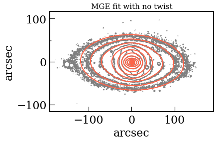
Figure 12: The contours of the NGC 4371 S⁴G image (grey lines), overplotted with contours of the best-fitting MGE without twist between different Gaussians applied to the whole galaxy.

$j$	$L_{j}$ $(\mathrm{L_{\odot}pc^{-2}})$	$\sigma^{\prime}_{j}$ $(\mathrm{arcsec})$	$q^{\prime}_{j}$	$\Delta\psi_{j}^{\prime}$ $(^{\circ})$
$1$	40257.908	1.35	0.74	0.0
$2$	4190.714	7.874	0.53	0.0
$3$	889.996	11.242	0.95	0.0
$4$	495.045	19.265	0.95	0.0
$5$	168.782	54.744	0.53	0.0
$6$	30.885	109.426	0.53	0.0

Table 3: Details of MGE fit for the whole galaxy in axisymmetric limit. $j$ is the number of each individual Gaussian for which, $L_{j}$ is the central flux in the unit of $(\mathrm{L_{\odot}pc^{-2}})$, $\sigma^{\prime}_{j}$ presents the size in the unit of $(\mathrm{arcsec})$, $q^{\prime}_{j}$ indicates the flattening. $\Delta\psi_{j}^{\prime}$ is twisted angle of Gaussian that is $0$ in this case.

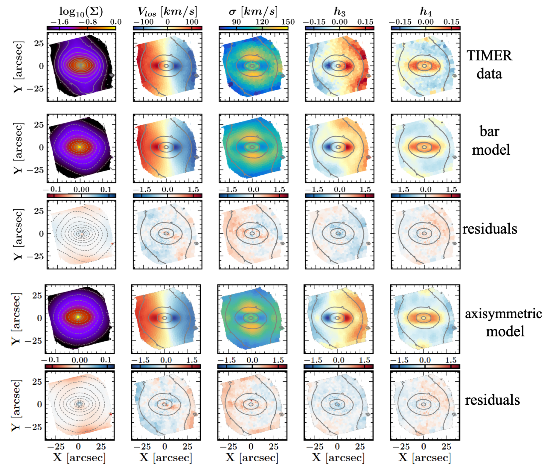
Figure 13: Comparison of the best-fitting bar model obtained with $\theta=59^{\circ}$ (second row) versus the best-fitting axisymmetric model (fourth row) obtained with $\theta=75^{\circ}$ using the TIMER data (first row). The third and fifth rows show the residual of each model. The surface density and its residuals are presented in the first column, for TIMER data, we use the flux of the IFU data cube and its contours, while for the bar and axisymmetric models, we used the MGEs surface density and its counters of the best-fitting models.

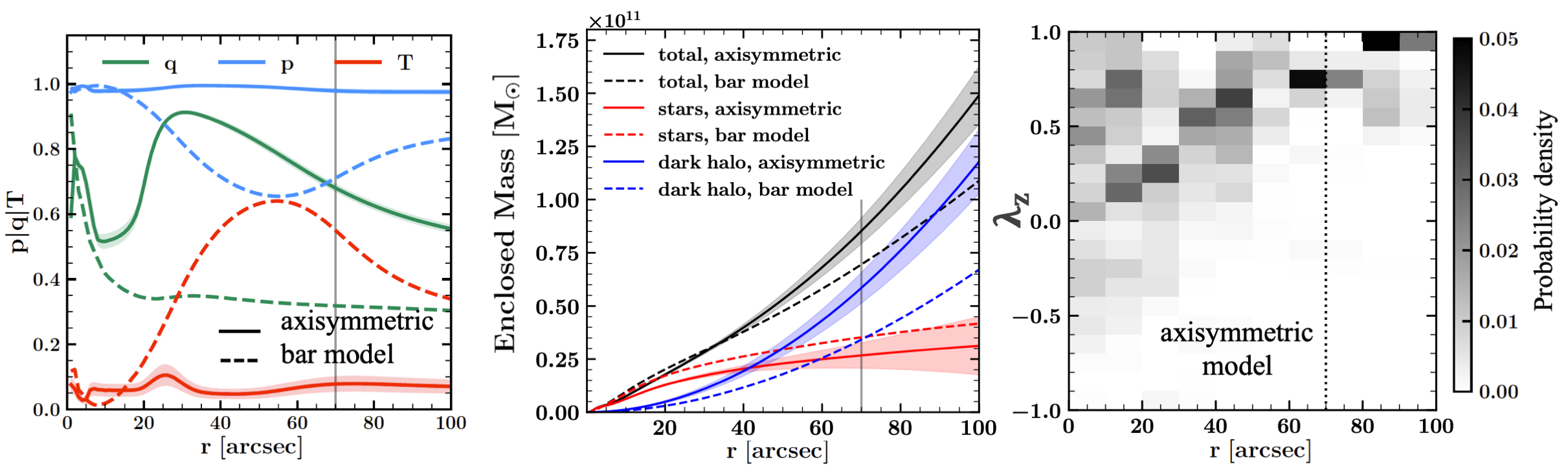
Figure 14: Left panel: variation of the axial ratios $q=c/a$ (green), $p=b/a$ (blue), and triaxial parameter $T=(1-p^{2})/(1-q^{2})$ (red) for the best-fitting axisymmetric model (solid lines) compared with the bar model (dashed lines) using TIMER. Middle panel: mass profiles of the best-fitting axisymmetric model (solid lines) compared with the bar model (dashed lines). The red, blue, and black curves represent the stellar mass, dark matter mass, and total mass, respectively. The shaded regions indicate the $1\sigma$ uncertainty from our axisymmetric models. The right panel represents the stellar orbit distribution in the space of circularity $\lambda_{z}$ vs. time-averaged radius $r$ for the best-fitting axisymmetric model with TIMER. The vertical dashed lines indicate the kinematics data extent.

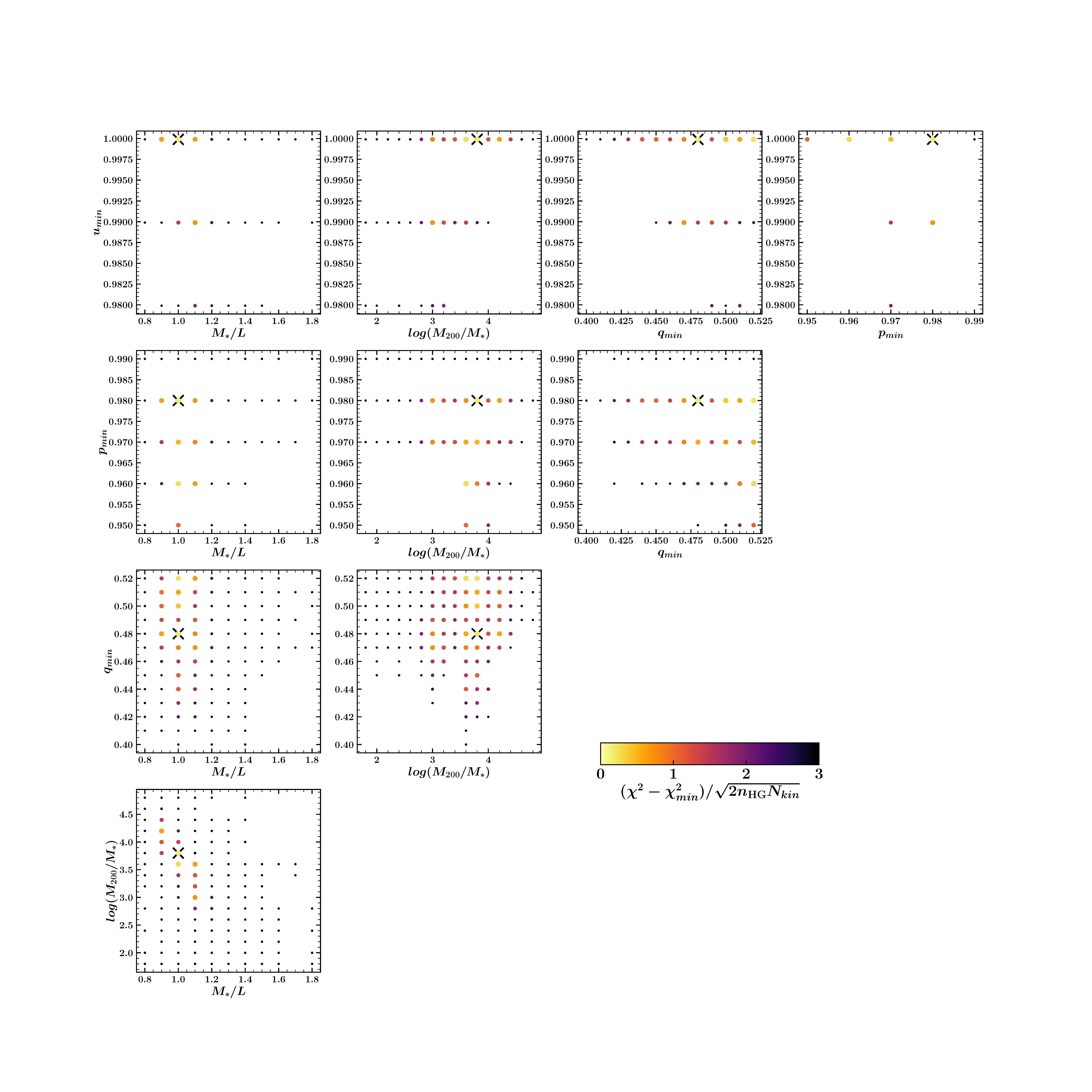
Figure 17: Same as Fig. 15 but for the axisymmetric model fitting using TIMER data. For the axisymmetric modeling, we use intrinsic parameters of $q,p,$ and $u$ instead of viewing angles of $\theta,\varphi,$ and $\psi$.

References

- Abbott et al. (2017) Abbott, C. G., Valluri, M., Shen, J., & Debattista, V. P. 2017, MNRAS, 470, 1526, doi: 10.1093/mnras/stx1262
- Aguerri et al. (1998) Aguerri, J. A. L., Beckman, J. E., & Prieto, M. 1998, AJ, 116, 2136, doi: 10.1086/300615
- Aguerri et al. (2015) Aguerri, J. A. L., Méndez-Abreu, J., Falcón-Barroso, J., et al. 2015, A&A, 576, A102, doi: 10.1051/0004-6361/201423383
- Athanassoula (2003) Athanassoula, E. 2003, MNRAS, 341, 1179, doi: 10.1046/j.1365-8711.2003.06473.x
- Athanassoula & Misiriotis (2002) Athanassoula, E., & Misiriotis, A. 2002, MNRAS, 330, 35, doi: 10.1046/j.1365-8711.2002.05028.x
- Bacon et al. (2001) Bacon, R., Copin, Y., Monnet, G., et al. 2001, MNRAS, 326, 23, doi: 10.1046/j.1365-8711.2001.04612.x
- Bacon et al. (2010) Bacon, R., Accardo, M., Adjali, L., et al. 2010, in Society of Photo-Optical Instrumentation Engineers (SPIE) Conference Series, Vol. 7735, Ground-based and Airborne Instrumentation for Astronomy III, ed. I. S. McLean, S. K. Ramsay, & H. Takami, 773508, doi: 10.1117/12.856027
- Binney & Tremaine (2008) Binney, J., & Tremaine, S. 2008, Galactic Dynamics: Second Edition (Princeton University Press)
- Bittner et al. (2019) Bittner, A., Falcón-Barroso, J., Nedelchev, B., et al. 2019, A&A, 628, A117, doi: 10.1051/0004-6361/20193582910.48550/arXiv.1906.04746
- Blaña Díaz et al. (2018) Blaña Díaz, M., Gerhard, O., Wegg, C., et al. 2018, MNRAS, 481, 3210, doi: 10.1093/mnras/sty2311
- Blakeslee et al. (2009) Blakeslee, J. P., Jordán, A., Mei, S., et al. 2009, ApJ, 694, 556, doi: 10.1088/0004-637X/694/1/556
- Bonnet et al. (2003) Bonnet, H., Ströbele, S., Biancat-Marchet, F., et al. 2003, in Society of Photo-Optical Instrumentation Engineers (SPIE) Conference Series, Vol. 4839, Adaptive Optical System Technologies II, ed. P. L. Wizinowich & D. Bonaccini, 329–343, doi: 10.1117/12.457060
- Breda et al. (2020) Breda, I., Papaderos, P., & Gomes, J.-M. 2020, A&A, 640, A20, doi: 10.1051/0004-6361/202037889
- Bundy et al. (2015) Bundy, K., Bershady, M. A., Law, D. R., et al. 2015, ApJ, 798, 7, doi: 10.1088/0004-637X/798/1/7
- Bureau & Athanassoula (2005) Bureau, M., & Athanassoula, E. 2005, ApJ, 626, 159, doi: 10.1086/430056
- Buta & Block (2001) Buta, R., & Block, D. L. 2001, ApJ, 550, 243, doi: 10.1086/319736
- Buta et al. (2015) Buta, R. J., Sheth, K., Athanassoula, E., et al. 2015, ApJS, 217, 32, doi: 10.1088/0067-0049/217/2/32
- Buttitta et al. (2022) Buttitta, C., Corsini, E. M., Cuomo, V., et al. 2022, A&A, 664, L10, doi: 10.1051/0004-6361/202244297
- Buttitta et al. (2023) Buttitta, C., Corsini, E. M., Aguerri, J. A. L., et al. 2023, MNRAS, 521, 2227, doi: 10.1093/mnras/stad646
- Cappellari (2002) Cappellari, M. 2002, MNRAS, 333, 400, doi: 10.1046/j.1365-8711.2002.05412.x
- Cappellari & Copin (2003) Cappellari, M., & Copin, Y. 2003, MNRAS, 342, 345, doi: 10.1046/j.1365-8711.2003.06541.x
- Cappellari & Emsellem (2004) Cappellari, M., & Emsellem, E. 2004, PASP, 116, 138, doi: 10.1086/38187510.48550/arXiv.astro-ph/0312201
- Cappellari et al. (2011) Cappellari, M., Emsellem, E., Krajnović, D., et al. 2011, MNRAS, 413, 813, doi: 10.1111/j.1365-2966.2010.18174.x
- Combes & Sanders (1981) Combes, F., & Sanders, R. H. 1981, A&A, 96, 164
- Croom et al. (2012) Croom, S. M., Lawrence, J. S., Bland-Hawthorn, J., et al. 2012, MNRAS, 421, 872, doi: 10.1111/j.1365-2966.2011.20365.x
- Cuomo et al. (2019a) Cuomo, V., Lopez Aguerri, J. A., Corsini, E. M., et al. 2019a, A&A, 632, A51, doi: 10.1051/0004-6361/201936415
- Cuomo et al. (2019b) Cuomo, V., Corsini, E. M., Aguerri, J. A. L., et al. 2019b, MNRAS, 488, 4972, doi: 10.1093/mnras/stz1943
- Cuomo et al. (2022) Cuomo, V., Corsini, E. M., Morelli, L., et al. 2022, MNRAS, 516, L24, doi: 10.1093/mnrasl/slac064
- Dattathri et al. (2023) Dattathri, S., Valluri, M., Vasiliev, E., Wheeler, V., & Erwin, P. 2023, arXiv e-prints, arXiv:2309.11557, doi: 10.48550/arXiv.2309.11557
- de Souza et al. (2004) de Souza, R. E., Gadotti, D. A., & dos Anjos, S. 2004, ApJS, 153, 411, doi: 10.1086/421554
- de Zeeuw & Franx (1989) de Zeeuw, T., & Franx, M. 1989, ApJ, 343, 617, doi: 10.1086/167735
- Debattista (2003) Debattista, V. P. 2003, MNRAS, 342, 1194, doi: 10.1046/j.1365-8711.2003.06620.x
- Debattista & Sellwood (1998a) Debattista, V. P., & Sellwood, J. A. 1998a, ApJ, 493, L5, doi: 10.1086/311118
- Debattista & Sellwood (1998b) —. 1998b, ApJ, 493, L5, doi: 10.1086/311118
- Debattista & Sellwood (2000) —. 2000, ApJ, 543, 704, doi: 10.1086/317148
- Ding et al. (2023) Ding, Y., Zhu, L., van de Ven, G., et al. 2023, A&A, 672, A84, doi: 10.1051/0004-6361/202244558
- Dullo et al. (2016) Dullo, B. T., Martínez-Lombilla, C., & Knapen, J. H. 2016, MNRAS, 462, 3800, doi: 10.1093/mnras/stw1868
- Dutton & Macciò (2014) Dutton, A. A., & Macciò, A. V. 2014, MNRAS, 441, 3359, doi: 10.1093/mnras/stu742
- Eisenhauer et al. (2003) Eisenhauer, F., Abuter, R., Bickert, K., et al. 2003, in Society of Photo-Optical Instrumentation Engineers (SPIE) Conference Series, Vol. 4841, Instrument Design and Performance for Optical/Infrared Ground-based Telescopes, ed. M. Iye & A. F. M. Moorwood, 1548–1561, doi: 10.1117/12.45946810.48550/arXiv.astro-ph/0306191
- Erwin (2018) Erwin, P. 2018, MNRAS, 474, 5372, doi: 10.1093/mnras/stx3117
- Erwin et al. (2008) Erwin, P., Pohlen, M., & Beckman, J. E. 2008, AJ, 135, 20, doi: 10.1088/0004-6256/135/1/20
- Erwin & Sparke (1999) Erwin, P., & Sparke, L. S. 1999, ApJ, 521, L37, doi: 10.1086/312169
- Erwin et al. (2015) Erwin, P., Saglia, R. P., Fabricius, M., et al. 2015, MNRAS, 446, 4039, doi: 10.1093/mnras/stu2376
- Eskridge et al. (2000) Eskridge, P. B., Frogel, J. A., Pogge, R. W., et al. 2000, AJ, 119, 536, doi: 10.1086/301203
- Falcón-Barroso et al. (2011) Falcón-Barroso, J., Sánchez-Blázquez, P., Vazdekis, A., et al. 2011, A&A, 532, A95, doi: 10.1051/0004-6361/20111684210.48550/arXiv.1107.2303
- Fisher & Drory (2010) Fisher, D. B., & Drory, N. 2010, ApJ, 716, 942, doi: 10.1088/0004-637X/716/2/942
- Fragkoudi et al. (2017) Fragkoudi, F., Di Matteo, P., Haywood, M., et al. 2017, A&A, 606, A47, doi: 10.1051/0004-6361/201630244
- Fragkoudi et al. (2021) Fragkoudi, F., Grand, R. J. J., Pakmor, R., et al. 2021, A&A, 650, L16, doi: 10.1051/0004-6361/202140320
- Gadotti (2008) Gadotti, D. A. 2008, MNRAS, 384, 420, doi: 10.1111/j.1365-2966.2007.12723.x
- Gadotti (2011) —. 2011, MNRAS, 415, 3308, doi: 10.1111/j.1365-2966.2011.18945.x
- Gadotti et al. (2007) Gadotti, D. A., Athanassoula, E., Carrasco, L., et al. 2007, MNRAS, 381, 943, doi: 10.1111/j.1365-2966.2007.12295.x
- Gadotti et al. (2015) Gadotti, D. A., Seidel, M. K., Sánchez-Blázquez, P., et al. 2015, A&A, 584, A90, doi: 10.1051/0004-6361/201526677
- Gadotti et al. (2019) Gadotti, D. A., Sánchez-Blázquez, P., Falcón-Barroso, J., et al. 2019, MNRAS, 482, 506, doi: 10.1093/mnras/sty2666
- Gadotti et al. (2020) Gadotti, D. A., Bittner, A., Falcón-Barroso, J., et al. 2020, A&A, 643, A14, doi: 10.1051/0004-6361/202038448
- Garma-Oehmichen et al. (2022) Garma-Oehmichen, L., Hernández-Toledo, H., Aquino-Ortíz, E., et al. 2022, MNRAS, 517, 5660, doi: 10.1093/mnras/stac3069
- Géron et al. (2023) Géron, T., Smethurst, R. J., Lintott, C., et al. 2023, MNRAS, 521, 1775, doi: 10.1093/mnras/stad501
- Guo et al. (2019) Guo, R., Mao, S., Athanassoula, E., et al. 2019, MNRAS, 482, 1733, doi: 10.1093/mnras/sty2715
- Jethwa et al. (2020) Jethwa, P., Thater, S., Maindl, T., & Van de Ven, G. 2020, DYNAMITE: DYnamics, Age and Metallicity Indicators Tracing Evolution, Astrophysics Source Code Library, record ascl:2011.007. http://ascl.net/2011.007
- Jin et al. (2020) Jin, Y., Zhu, L., Long, R. J., et al. 2020, MNRAS, 491, 1690, doi: 10.1093/mnras/stz3072
- Kim et al. (2014) Kim, T., Gadotti, D. A., Sheth, K., et al. 2014, ApJ, 782, 64, doi: 10.1088/0004-637X/782/2/6410.48550/arXiv.1312.3384
- Kormendy & Ho (2013) Kormendy, J., & Ho, L. C. 2013, ARA&A, 51, 511, doi: 10.1146/annurev-astro-082708-10181110.48550/arXiv.1304.7762
- Kormendy & Kennicutt (2004) Kormendy, J., & Kennicutt, Robert C., J. 2004, ARA&A, 42, 603, doi: 10.1146/annurev.astro.42.053102.134024
- Lawson & Hanson (1974) Lawson, C. L., & Hanson, R. J. 1974, Solving least squares problems
- Li & Shen (2012) Li, Z.-Y., & Shen, J. 2012, ApJ, 757, L7, doi: 10.1088/2041-8205/757/1/L7
- Li et al. (2018) Li, Z.-Y., Shen, J., Bureau, M., et al. 2018, ApJ, 854, 65, doi: 10.3847/1538-4357/aaa771
- Lipka & Thomas (2021) Lipka, M., & Thomas, J. 2021, MNRAS, 504, 4599, doi: 10.1093/mnras/stab1092
- Long et al. (2013) Long, R. J., Mao, S., Shen, J., & Wang, Y. 2013, MNRAS, 428, 3478, doi: 10.1093/mnras/sts285
- Lütticke et al. (2000) Lütticke, R., Dettmar, R. J., & Pohlen, M. 2000, A&AS, 145, 405, doi: 10.1051/aas:2000354
- Meidt et al. (2014) Meidt, S. E., Schinnerer, E., van de Ven, G., et al. 2014, ApJ, 788, 144, doi: 10.1088/0004-637X/788/2/144
- Méndez-Abreu et al. (2014) Méndez-Abreu, J., Debattista, V. P., Corsini, E. M., & Aguerri, J. A. L. 2014, A&A, 572, A25, doi: 10.1051/0004-6361/201423955
- Navarro et al. (1996) Navarro, J. F., Frenk, C. S., & White, S. D. M. 1996, ApJ, 462, 563, doi: 10.1086/177173
- Parul et al. (2020) Parul, H. D., Smirnov, A. A., & Sotnikova, N. Y. 2020, ApJ, 895, 12, doi: 10.3847/1538-4357/ab76ce
- Peng et al. (2010) Peng, C. Y., Ho, L. C., Impey, C. D., & Rix, H.-W. 2010, AJ, 139, 2097, doi: 10.1088/0004-6256/139/6/2097
- Poci et al. (2019) Poci, A., McDermid, R. M., Zhu, L., & van de Ven, G. 2019, MNRAS, 487, 3776, doi: 10.1093/mnras/stz1154
- Portail et al. (2017) Portail, M., Gerhard, O., Wegg, C., & Ness, M. 2017, MNRAS, 465, 1621, doi: 10.1093/mnras/stw2819
- Portail et al. (2015) Portail, M., Wegg, C., & Gerhard, O. 2015, MNRAS, 450, L66, doi: 10.1093/mnrasl/slv048
- Raha et al. (1991) Raha, N., Sellwood, J. A., James, R. A., & Kahn, F. D. 1991, Nature, 352, 411, doi: 10.1038/352411a0
- Saglia et al. (2016) Saglia, R. P., Opitsch, M., Erwin, P., et al. 2016, ApJ, 818, 47, doi: 10.3847/0004-637X/818/1/47
- Sánchez et al. (2012) Sánchez, S. F., Kennicutt, R. C., Gil de Paz, A., et al. 2012, A&A, 538, A8, doi: 10.1051/0004-6361/201117353
- Sánchez-Blázquez et al. (2006) Sánchez-Blázquez, P., Peletier, R. F., Jiménez-Vicente, J., et al. 2006, MNRAS, 371, 703, doi: 10.1111/j.1365-2966.2006.10699.x10.48550/arXiv.astro-ph/0607009
- Santucci et al. (2022) Santucci, G., Brough, S., van de Sande, J., et al. 2022, ApJ, 930, 153, doi: 10.3847/1538-4357/ac5bd5
- Schwarzschild (1979) Schwarzschild, M. 1979, ApJ, 232, 236, doi: 10.1086/157282
- Sheth et al. (2010) Sheth, K., Regan, M., Hinz, J. L., et al. 2010, PASP, 122, 1397, doi: 10.1086/65763810.48550/arXiv.1010.1592
- Tahmasebzadeh et al. (2021) Tahmasebzadeh, B., Zhu, L., Shen, J., Gerhard, O., & Qin, Y. 2021, MNRAS, 508, 6209, doi: 10.1093/mnras/stab3002
- Tahmasebzadeh et al. (2022) Tahmasebzadeh, B., Zhu, L., Shen, J., Gerhard, O., & Ven, G. v. d. 2022, ApJ, 941, 109, doi: 10.3847/1538-4357/ac9df6
- Thater et al. (2022) Thater, S., Jethwa, P., Tahmasebzadeh, B., et al. 2022, A&A, 667, A51, doi: 10.1051/0004-6361/202243926
- Tremaine & Weinberg (1984) Tremaine, S., & Weinberg, M. D. 1984, ApJ, 282, L5, doi: 10.1086/184292
- Valluri & Merritt (1998) Valluri, M., & Merritt, D. 1998, ApJ, 506, 686, doi: 10.1086/306269
- Valluri et al. (2016) Valluri, M., Shen, J., Abbott, C., & Debattista, V. P. 2016, ApJ, 818, 141, doi: 10.3847/0004-637X/818/2/141
- van den Bosch et al. (2008) van den Bosch, R. C. E., van de Ven, G., Verolme, E. K., Cappellari, M., & de Zeeuw, P. T. 2008, MNRAS, 385, 647, doi: 10.1111/j.1365-2966.2008.12874.x
- Vasiliev & Valluri (2020) Vasiliev, E., & Valluri, M. 2020, ApJ, 889, 39, doi: 10.3847/1538-4357/ab5fe0
- Wang et al. (2013) Wang, Y., Mao, S., Long, R. J., & Shen, J. 2013, MNRAS, 435, 3437, doi: 10.1093/mnras/stt1537
- Zhu et al. (2018a) Zhu, L., van de Ven, G., van den Bosch, R., et al. 2018a, Nature Astronomy, 2, 233, doi: 10.1038/s41550-017-0348-1
- Zhu et al. (2018b) Zhu, L., van den Bosch, R., van de Ven, G., et al. 2018b, MNRAS, 473, 3000, doi: 10.1093/mnras/stx2409
- Zhu et al. (2020) Zhu, L., van de Ven, G., Leaman, R., et al. 2020, MNRAS, 496, 1579, doi: 10.1093/mnras/staa1584
- Zhu et al. (2022) —. 2022, A&A, 664, A115, doi: 10.1051/0004-6361/202243109
- Zou et al. (2019) Zou, Y., Shen, J., Bureau, M., & Li, Z.-Y. 2019, ApJ, 884, 23, doi: 10.3847/1538-4357/ab3f34