Better Situational Graphs by Inferring High-level
Semantic-Relational Concepts

Abstract

Recent works on SLAM extend their pose graphs with higher-level semantic concepts exploiting relationships between them, to provide, not only a richer representation of the situation/environment but also to improve the accuracy of its estimation. Concretely, our previous work, Situational Graphs (S-Graphs), a pioneer in jointly leveraging semantic relationships in the factor optimization process, relies on semantic entities such as wall surfaces and rooms, whose relationship is mathematically defined. Nevertheless, excerpting these high-level concepts relying exclusively on the lower-level factor-graph remains a challenge and it is currently done with ad-hoc algorithms, which limits its capability to include new semantic-relational concepts.

To overcome this limitation, in this work, we propose a Graph Neural Network (GNN) for learning high-level semantic-relational concepts that can be inferred from the low-level factor graph. We have demonstrated that we can infer room entities and their relationship to the mapped wall surfaces, more accurately and more computationally efficient than the baseline algorithm. Additionally, to demonstrate the versatility of our method, we provide a new semantic concept, i.e. wall, and its relationship with its wall surfaces. Our proposed method has been integrated into S-Graphs+, and it has been validated in both simulated and real datasets. A docker container with our software will be made available to the scientific community.

I Introduction

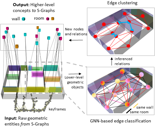
Figure 1: System Overview. We augment the original S-Graph from our SLAM system [1] with additional constraints derived from higher-level information like relations between walls and rooms. Taking low-level concepts like wall surfaces as graph nodes, a trained graph neural network (GNN) classifies which relations belong to the same room or same wall and decides which constraints are then added to the S-Graph to improve the quality of the map and the estimated camera trajectory.

Incorporating higher-level semantic-relational entities enhances the situational awareness [2] of a robot and hence enriches the built model of the world. Furthermore, it provides advantageous information for successive tasks such as planning [3].

Graph-based SLAM optimizes a graph with real-world objects observed from measurements and only geometric and temporal information. During recent years, 3D Semantic Scene Graphs [4, 5, 6] emerged as a promising framework to associate the SLAM graph structure with higher-level semantic-relational concepts. [7] goes beyond and optimizes the conjunction graph leveraging loop closures.

Our previous work S-Graphs [1] fully integrates the SLAM graph with the scene graph optimizing them as a unified entity. However, S-Graphs only extracts a few semantic-relational entities and these semantic-relational entities are extracted with ad-hoc algorithms per entity type, limiting the capability of S-Graphs to generalize to different and complex type of semantic entities.

To address these limitations, we present a framework to enhance S-Graphs with relational and generalization capabilities over semantic entities based on GNNs [8, 9]. Our framework can infer pairwise relationships among wall surfaces belonging to the same higher-level entities either walls or rooms. These relationships are subsequently processed and clustered in the set of nodes relating to the new entity.

Furthermore, these newly generated entities along with their relationships are incorporated as nodes and edges into the appropriate layers of the four-layered optimizable S-Graph. The results over several simulated and real structured indoor environments demonstrate that our method improves the baseline in detection time, expressiveness, and the number of entities detected. Refer to Fig. 1 for a visual representation of our system.

To summarize, the primary contributions of our paper are:

• A GNN-based framework to generate high-level semantic entities (concretely, rooms and walls) and their relationships from the low-level entities (i.e. wall surfaces) in a computationally efficient and versatile manner.

• Integration of the algorithm within the four-layered optimizable S-Graphs framework [1] along with validation in simulated and real datasets with ablation studies.

II Related work

II-A Semantic Scene Graphs for SLAM

Scene graphs serve as graph models that encapsulate the environment as structured representations. This graph comprises entities, their associated attributes, and the interrelationships among them. In the context of 3D scene graphs,[4] has pioneered the development of an offline, semi-autonomous framework. This framework relies upon object detections derived from RGB images, creating a multi-layered hierarchical representation of the environment and its constituent elements such as cameras, objects, rooms, and buildings. Additionally,[5] employs a sequence of images for visual questioning and answering and planning.

GNNs [8, 9] have been proposed to deduce scene graphs from images [10, 11], where the entities within the scene constitute the nodes of the graph, specifically object instances. Scene graph prediction necessitates the incorporation of relationships between these instances. [12] presented an initial large-scale 2D scene graph dataset, while  [13, 14, 15], have extended the concept to generate 3D semantic scene graph annotations within indoor and outdoor environments, including object semantics, rooms, cameras, and the relationships interconnecting these entities. [16] extends this model to dynamic entities as humans. Furthermore, [6] does not need any prior scene knowledge and segments instances, their semantic attributes, and the concurrent inference of relationships, all in real-time.

While all these frameworks run SLAM in the background, they do not utilize the scene graph to enhance the SLAM process. Hydra[7] focuses on real-time 3D scene graph generation and optimization using loop closure constraints. [17] introduces the concept of Neural Trees, H-Tree, as an evolution from GNNs where message-passing nodes within the graph correspond to subgraphs within the input graph, and they are organized hierarchically, effectively enhancing the expressive capacity of GNNs. The extension of Hydra in [18] introduces H-Tree to enhance the characterization of specific building areas, like kitchens. However, they do not integrate the SLAM state with the scene graph for simultaneous optimization.

Our prior works S-Graphs[19, 1], successfully bridged the gap by demonstrating the potential of tightly integrating SLAM graphs and scene graphs. S-Graphs creates a four-layered hierarchical optimizable graph while concurrently representing the environment as a 3D scene graph, achieving remarkable performance even in complex settings. Furthermore, we have expanded its capabilities by hierarchically selecting regions of the graph to optimize[20], incorporating prior architectural information[21], visual fiducial markers[22], or collaborative data from multiple robots[23]. It has also been employed to formulate a navigation problem[3]. In this work, our objective is to harness the capabilities of GNNs to enhance all these research directions by generating more reliable, versatile, and comprehensive higher-level representations within S-Graphs.

II-B Room and Wall Detection

The first step in the generation of higher-level concepts resides in comprehending the interrelations among fundamental geometric entities. The identification of structural configurations corresponding to wall surfaces which collectively form rooms and walls, is crucial. Various methods have been explored to address this challenge, encompassing the utilization of pre-existing 2D LiDAR maps[24, 25, 26], the utilization of 2D occupancy maps within complex indoor environments[27], and pre-established 3D maps[28, 29, 30]. It should be noted, however, that these approaches exhibit inherent performance constraints and lack real-time operational capabilities.[7] introduce a real-time room segmentation approach designed to classify different places into rooms. In [1], we leverage the wall surfaces contained in the S-Graphs+ to instantaneously define rooms in real-time, while concurrently incorporating these findings into the optimizable graph. To the best of our knowledge, no analogous methodologies exist for the automated identification of wall entities.

III Methodology

The pipeline of our method is illustrated in Fig. 2. First, the low-level layer of S-graph, i.e. the mapped keyframe and wall surface, is received, extracting only the wall surface nodes. Then, the features of those nodes are preprocessed to build a proximity graph and define the initial embedding of nodes and edges, as described in Sec. III-A. Next, node and edge embeddings are updated to infer a classification in every edge, as presented in Sec. III-B. Later, the inferred edges are clustered, and new nodes for the new wall and room entities are generated, introducing along with them, a link with the wall surface nodes, following the method proposed in Sec. III-C. Finally, the new nodes and relationships are integrated as the high-level layers of S-Graphs.

Figure 2: System Architecture. The entire process from geometric entities reception to the inclusion of new higher-level entities to S-Graph. a) The low-level layer of S-Graph is received. b) Only nodes of interest are selected i.e. the wall surfaces. c) A proximity graph for message passing is created amongst the nodes and the initial features of edges and nodes are computed from incoming node definitions. d) A GNN for nodes and linear layers for edges are employed to update embeddings via message sharing. e) Both embedding types are used to classify edges through linear layers. f) Edges are consistently grouped. g) For each group, a new node is created and linked with the clustered nodes. h) The new semantic nodes and links are added to the original S-Graph.

III-A Initial Graph

Initially, raw wall surfaces in S-Graphs+ are defined as a point cloud and a normal, which describes the observation side. To simplify this representation, points are flattened and assimilated to a 2D line. Subsequently, overlapping lines are filtered out and intersecting lines are split to overcome the issue of a unique long wall surface belonging to various rooms. Finally, the initial node embedding $v^{0}_{i}$ is defined as $[w_{i},n_{i}]$ where $w_{i}$ is the width of the wall surface and $n_{i}$ is the normal from the observed side.

At this point, we have a set of clean nodes without a graph structure. Hence, new directed edges are artificially created in the message-passing graph by node proximity. See Fig. 2.B. The initial embedding of those new edges, $e^{0}_{ij}$, is defined as $[c_{j}-c_{i},cd_{ij}]$ where $cd_{ij}$ is the closest distance and $c_{i}$ is the centroid of the $i_{th}$ node.

III-B Embedding Update and Classification

Inspired by [6], the classification process follows an encoder-decoder fashion. The encoder updates the node and edge embeddings separately but interleaved using the latest updates as in Eq. (1) and Eq. (2).

$$v_{i}^{l+1} =g_{v}\big{(}\big{[}v_{i}^{l},\max_{j\in\mathcal{N}(i)}(\mathrm{GAT}(v_{i}^{l},e_{ij}^{l},v_{j}^{l}))\big{]}\big{)}$$ (1)

$$e_{ij}^{l+1} =g_{e}([v_{i}^{l},e_{ij}^{l},v_{j}^{l}])$$ (2)

where $g_{v}(\cdot)$ and $g_{e}(\cdot)$ are linear layers [31], $\mathcal{N}(i)$ are the neighbors of $i_{th}$ node and $\mathrm{GAT}(\cdot)$ is a Graph Attention Network [8, 9]. Encoder hyperparameters are maintained across the classification of both classes. Two layers of Eq. (1) and Eq. (2) are used.

As opposed to encoder, decoder hyperparameters are specific to the target class. The outcome of the Encoder is passed through a multi-layer perceptron as in Eq. (3) before the final binary classification of a specific edge.

$$c_{ij}=g_{d}([v_{i}^{L},e_{ij}^{L},v_{j}^{L}])$$ (3)

where $g_{d}(\cdot)$ are three linear layers and $L$ is the last layer of the encoder.

Input: wall surface nodes and same room edges graph $\mathcal{G}_{WS}$

Output: Clustering as list of node lists $\boldsymbol{\mathcal{V}_{R}}$

$\boldsymbol{\mathcal{V}_{R}}\leftarrow[]$

for $l_{i}\in\boldsymbol{N}_{WS}$ do

       $\boldsymbol{\mathcal{E}_{c}}\leftarrow find\_cycles\_of\_size\_l(\mathcal{G}_{WS},l_{i})$

       $\boldsymbol{\mathcal{V}_{ini}}\leftarrow\mathcal{E}_{c,j}.nodes\ \forall\ \mathcal{E}_{c,j}\in\boldsymbol{\mathcal{E}_{c}}$

       $\mathcal{I}_{count}\leftarrow count\_set\_repetitions(\boldsymbol{\mathcal{V}_{ini}})$

       $\boldsymbol{\mathcal{V}_{sort}}\leftarrow sort\_descendent(\boldsymbol{\mathcal{V}_{ini}},\mathcal{I}_{count})$

      

      for $\mathcal{V}_{sort,j}\in\boldsymbol{\mathcal{V}_{sort}}$ do

             if $all(\mathcal{V}_{sort,j}\notin\boldsymbol{\mathcal{V}_{R}})$ then

                   $\boldsymbol{\mathcal{V}_{R}}.append(\mathcal{V}_{sort,j})$

                   $\mathcal{G}_{WS}.remove(\mathcal{V}_{sort,j})$

                  

             end if

            

       end for

      

end for

Algorithm 1 same room edge clustering

III-C Subgraph Generation

Each set of predicted relations, same room and same wall, follows a different clustering process to generate rooms and walls nodes. On one hand, since wall is composed of two wall surfaces, only one inferred same wall relation is required to obtain a cluster of two wall surface nodes.

On the other hand, for same room relationship, the existence of cycles is leveraged to select wall surface nodes that appear in the higher number of cycles, as explained in Algorithm. 1. We assume all wall surface nodes forming a same room relationship are connected through at least one cycle. As rooms can vary in the number of wall surfaces contained, cycles of that length are found in a descendent order, prioritizing bigger rooms. For each length, a set of wall surface nodes defined by the largest cycle are prioritized. However, even though any number of wall sufraces could be associated with a room, only sets linked to two and four are generated, since currently, S-Graphs+ only contains those factor types. Since the same node cannot be part of two different rooms, every selected set of nodes is removed from the initial graph and the process is repeated for smaller rooms. This overcomes the issue of the existence of false positives that may lead to the merging of wall surfaces of two different rooms.

Finally, the newly generated nodes (rooms, walls) along with the respective wall surface nodes are incorporated into the Rooms layer of the optimizable S-Graph. For room nodes, the factor already present in S-Graphs as described in [1] is utilized. Whereas for wall nodes, the factor employed is presented in [21].

IV Training with synthetic dataset

Due to the lack of an existing tagged dataset in the literature that provides the targeted entities and relationships, we have developed a synthetic one focused on replicating the common wall surface structure of usual indoor environments. To create replicate data as similar as possible to the observed S-Graphs+, the data is augmented with several layers of randomization in size, position, and orientation when creating rooms and wall surfaces. Ground truth edges are automatically tagged as same room or same wall and included along with negative tagged message passing edges with the 15 closest neighbor nodes for each node. During the training process, 800 different layouts are used for backpropagation during each one of the 35 epochs. Xavier uniform initialization [32] is used for the learnable parameters. Fig. 3 shows an example of inference in this dataset after training. After the initial training with the synthetic dataset, the model is used on real data without further training, with no additional tuning of parameters and the same normalization applied.

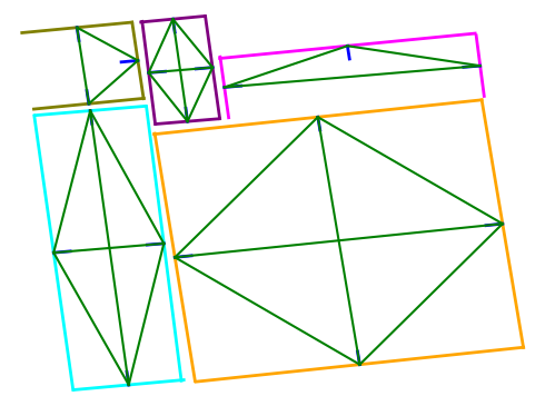
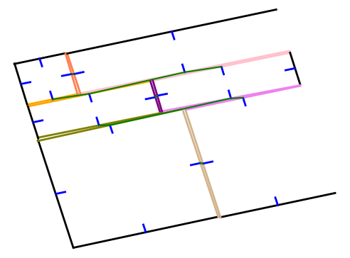
(a) same room inference	(b) same wall inference

Figure 3: Training performance of our approach on our synthetic dataset. Green lines represent edges inferred as positive for the respective relation. Black lines represent wall surfaces not included in a cluster. For the rest of the entities, those with the same color are grouped in the same cluster. Note that some wall surfaces are omited to simulate occlusions.

V Experimental Results

V-A Methodology

Our work is validated across multiple construction sites and office spaces, both simulated and real-world scenarios, as detailed in Tab. I and [1]. We compare it with the ad-hoc room detection algorithm presented in S-Graphs+ [1] which we name Free Space. Furthermore, we ablate our method tagged as Ours (rooms only) standing for inference without walls. VLP-16 LiDAR data is utilized across all datasets. The example scenarios are tagged with either s or r to differentiate simulation and real respectively.

In all the experiments, no fine-tuning of the specified network hyper-parameters is applied, as the empirically chosen ones suffice for all cases.

Simulated Data. We performed a total of five experiments on simulated datasets denoted as C1F1s, C1F2s, SE1s, SE2s, and SE3s. C1F1s and C1F2s are generated from the 3D meshes of two floors of actual architectural plans, while SE1, SE2s and SE23s simulate typical indoor environments with varying room configurations. In order to assess the tracking and mapping performance of our pipeline with and without our S-Graph augmentation, our reported metrics include Average Trajectory Error (ATE) and Map Matching Accuracy (MMA), and the evaluations are conducted against the ground truth provided by the simulator. Due to the absence of odometry from robot encoders, the odometry is solely estimated from LiDAR measurements in all simulated experiments.

Real Dataset. We conducted four experiments in two different construction sites. C1F1r and C1F2r are conducted on two floors of a construction site whose plan is used in the simulated dataset. C2F2r and C3F2r are conducted in two other construction sites. To validate the accuracy of each method in all real-world experiments, we report the MMA of the estimated 3D maps in comparison to the actual 3D map generated from the architectural plan. We employ robot encoders for odometry estimation.

TABLE I: Scenes description. Enumeration of all simulated and real scenes included in the validation. Room shapes can be squared, L-shaped, elongated or corridors.

Scene	World	Description
C1F1s	Simulated	1 L-shaped, 1 squared rooms and 2 corridors.
C1F2s	Simulated	5 squared, 2 elongated rooms and 1 corridor.
SE1s	Simulated	6 squared rooms and 3 corridors.
SE2s	Simulated	5 squared and 2 elongated rooms.
SE3s	Simulated	22 squared rooms and 4 corridors.
C1F1r	Real	1 L-shaped, 1 squared rooms and 2 corridors.
C1F2r	Real	5 squared, 2 elongated rooms and 1 corridor.
C2F2r	Real	7 squared, 2 L-shaped and 3 elongated rooms.
C3F2r	Real	9 squared, 3 L-shaped rooms and 2 corridors.

V-B Results and Discussion

Average Trajectory Error. The ATE for the simulated experiments is presented in Tab. II. S-Graphs+ with our approach for room and wall detection demonstrates an improvement of 6.8% with respect to S-Graphs+ with Free Space for rooms. The ablation of walls in Ours (rooms only) shows an improvement of 5.2% even though no new entity types are leveraged. Note that in construction sites more complex and similar to real data, C1F1s, C1F2s and SE3, our approach is capable of dealing better with edge cases. See examples in Fig. 5. However, when complexity and size decrease, Free Spaces presents a better performance.

TABLE II: Absolute Trajectory Error (ATE) [m], of S-Graph+ with different detection modules on simulated data. Best results are boldfaced. Both of our approaches improve the ATE of the baseline in the most complex scenes Considering semantic relations between both walls and room is always better or equal than only rooms.

	Dataset [m $\times 10^{-2}$]
Module	C1F1s	C1F2s	SE1s	SE2s	SE3s	Avg
Free Space [1] (baseline)	2.70	6.93	1.47	1.36	2.98	3.09
Ours (rooms only)	2.72	6.58	1.55	1.57	2.23	2.93
Ours	2.71	6.35	1.54	1.56	2.23	2.88

Map Matching Accuracy. Tab. III presents the point cloud RMSE for simulated and real experiments. S-Graphs with our approach for room and wall detection presents an improvement of 1.8% with respect to S-Graphs with Free Space for rooms. In this case, the ablation of walls in Ours (rooms only) still represents an improvement of 0.3% when only the same entity type of the baseline is used. The results demonstrate that, even the MMA was already low in the baseline, in inclusion of better and new factors to S-Graphs+ still represents a notable improvement.

TABLE III: Map Matching Accuracy (MMA) [m] of S-Graphs+ with different detection modules on simulated and real data. Best results are boldfaced. In all real scenes and in all but one simulated, the MMA is outperformed by our approach, including the ablated method.

	Dataset [m $\times 10^{-2}$]
Module	SE2s	C1F1s	C1F2s	C1F1r	C1F2r	C2F2r	C3F2r	Avg
Free Space [1]	27.53	7.40	7.55	32.60	18.75	17.8	44.86	22.35
Ours (rooms only)	27.52	7.61	7.53	32.54	18.64	17.8	44.35	22.28
Ours	27.51	7.60	7.51	32.67	17.79	17.27	43.31	21.95

Precision/Recall. Fig. 4 showcases the performance on the detection of rooms for simulated and real scenarios. Free Space is compared with our ablated module (rooms only). On average, precision is maintained slightly over Free Space. Note that it is over 80% in all simulated sites and all real ones but one. Recall average is also maintained, although both methods experience a descent in performance. This is due to detections being heavily dependent on the layout of the building and the GNN could not generalize properly enough from the training dataset.

On its side, wall detection can not be compared due to the lack of an analogous baseline. The results in the performance are presented in Tab. IV. It is worth mentioning that precision is maintained at 1.00 along every simulated and real scene. Recall is over 75% in all scenes but in a simulated one. On the contrary to rooms, the shape of all walls present a low variability. It reduces the complexity for the generalization increasing the performance.

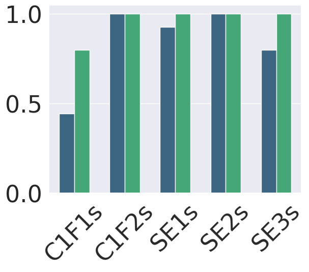
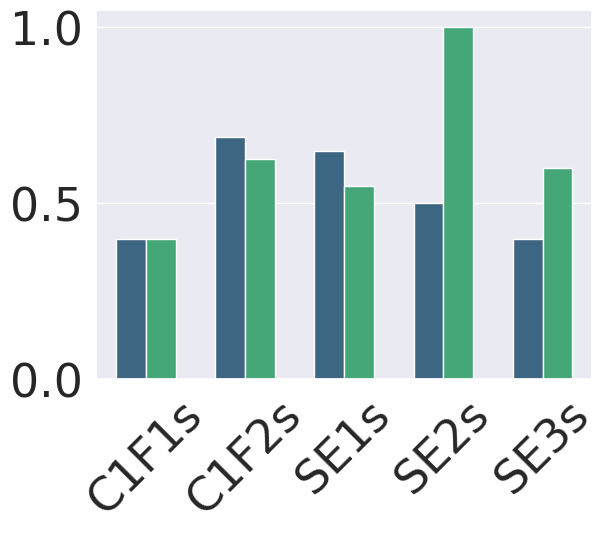
(a) Simulation, precision	(b) Simulation, recall
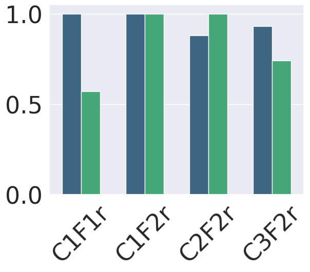
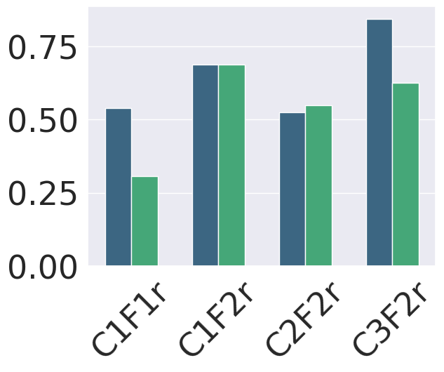
(c) Real, precision	(d) Real, recall

Figure 4: Precision and recall in room detection for Free Space  [1] (blue) and our approach (green) in 9 different simulated and real scenes. In simulated scenes, precision and recall are plainly improved by our method, while in real scenes there is more variability due to the larger amount of noise.

TABLE IV: Normalized precision and recall in wall detection of our approach in different simulated and real scenes. The precision is maintained at 1.00 for every site. The recall is over 0.75 but in one edge case in simulation.

	Dataset
Metric	C1F1s	C1F2s	SE1s	SE2s	SE3s	Avg
Precision	1.00	1.00	1.00	1.00	1.00	1.00
Recall	0.80	1.00	0.87	0.43	0.89	0.80
	C1F1r	C1F2r	C2F2r	C3F2r		Avg
Precision	1.00	1.00	1.00	1.00		1.0
Recall	0.80	0.75	0.82	0.84		0.80

First Detection Time. Additionally, Tab. V provides a comprehensive overview of the time required by each module to accomplish detection of the first room. Every experiment is started inside the construction site, that is inside of a room. Free Space is compared with our ablated module (rooms only), demonstrating a drastic average improvement of 84.3% in the simulated dataset and 62.7% in the real dataset. Note that the detection time drastically decreases in all cases. This is due to the need of Free Space to observe many points until a cluster is inferred while our method succeeds in the first observation half of the time.

TABLE V: First Detection Time (FDT) [s] of rooms employing S-Graphs+ with different detection modules on simulated and real data. Our method is substantially faster than the baseline. Best results are boldfaced.

	Dataset
	Computation Time (mean) [ms]
Module	C1F1s	C1F2s	SE1s	SE2s	SE3s	Avg
Free Space [1] (baseline)	76.0	19.0	19.0	115.0	160.0	77.8
Ours	2.7	2.8	10.2	8.2	37.1	12.2
	C1F1r	C1F2r	C2F2r	C3F2r		Avg
Free Space [1] (baseline)	19.0	25.5	367.0	308.0		179.9
Ours	1.7	2.6	54.0	210.2		67.1

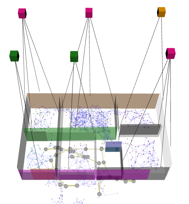
(a) Free Space [1] in SE2s

(b) Ours in SE2s

(c) Free Space [1] in SE3s

(d) Ours in SE3s

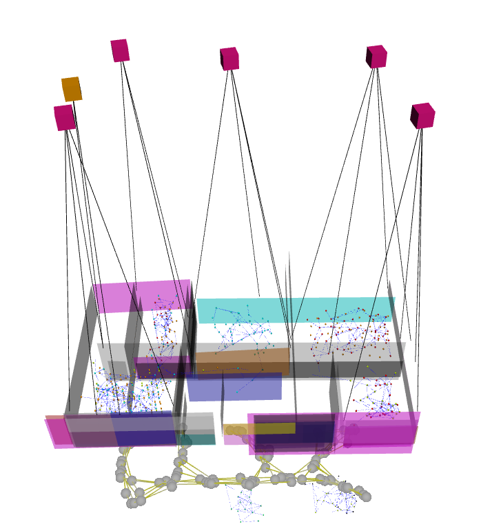
(e) Free Space [1] in C1F2r

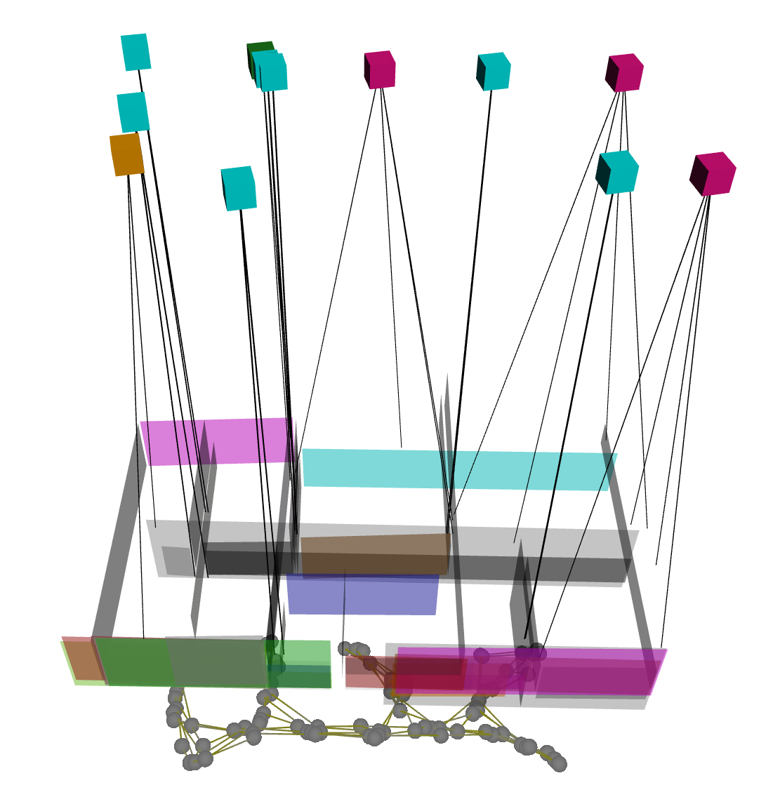
(f) Ours in C1F2r

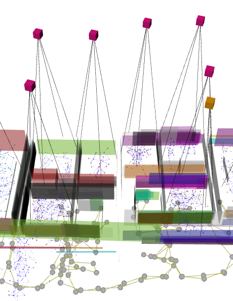
(g) Free Space [1] in C2F2r

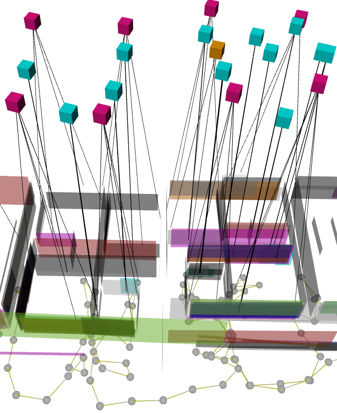
(h) Ours in C2F2r

Figure 5: Complete final S-Graph after Free Space [1] and Ours higher-level entity detections in real and simulated environments. In both of the generations of our method, the room (pink, orange and green cubes) density is higher. Furthermore, only in our approach, wall nodes (blue cubes) are generated. The first two examples show the performance in simulated scenes and the last two, in real scenes. Note the difference from our approach (right column) compared to free space (left column) in the density of inferred rooms. Also, note that walls are only inferred by our method.

Limitations. Although our experiments demonstrate that the augmentation of the S-Graph with semantic relation improves both map and trajectory estimation performance, the training for identifying related walls and rooms is separate from these improvement goals. The exact dependency between a better labeling performance of the GNN and the final mapping and tracking scores is not fully explored.

VI Conclusion

We presented a novel approach for the detection of rooms and walls using Graph Neural Networks to enrich the scene graph utilized by S-Graphs+ in the context of SLAM. Our method unfolds in several steps: (a) Edge Inference: Initially, we infer same room and same wall edges among the wall surface nodes already present in S-Graphs+. (b) Clustering: Subsequently, we process these inferred edges to cluster nodes corresponding to each higher-level concept. (c) Subgraph Creation: Finally, we represent these clusters in the form of a subgraph, incorporating it into the existing factors employed in S-Graphs+, and seamlessly integrate it into the scene graph for optimization.

In comparison to the current algorithm used for rooms, and given that walls are not yet automatically detected, our approach exhibits notable enhancements in terms of detection time, expressiveness, and generalization attributes. Importantly, these improvements do not compromise the performance of trajectory estimation and mapping.

In future research, our primary objective is to learn the optimal new graph in an end-to-end manner, leveraging the actual performance of the SLAM optimization as feedback. This approach would generate the entire new subgraph, factors included, as the outcome of the GNN process, thereby obviating the necessity for manually crafted rules. We also aim to expand the range of relations we can infer and hence augment the node and edge types integrated into S-Graphs.

References

- [1] H. Bavle, J. L. Sanchez-Lopez, M. Shaheer, J. Civera, and H. Voos, “S-graphs+: Real-time localization and mapping leveraging hierarchical representations,” IEEE Robotics and Automation Letters, 2023.
- [2] H. Bavle, J. L. Sanchez-Lopez, C. Cimarelli, A. Tourani, and H. Voos, “From slam to situational awareness: Challenges and survey,” Sensors, vol. 23, no. 10, 2023. [Online]. Available: https://www.mdpi.com/1424-8220/23/10/4849
- [3] P. Kremer, H. Bavle, J. L. Sanchez-Lopez, and H. Voos, “S-nav: Semantic-geometric planning for mobile robots,” arXiv preprint arXiv:2307.01613, 2023.
- [4] I. Armeni, Z.-Y. He, J. Gwak, A. R. Zamir, M. Fischer, J. Malik, and S. Savarese, “3D Scene Graph: A structure for unified semantics, 3D space, and camera,” in Proceedings of the IEEE/CVF International Conference on Computer Vision, 2019, pp. 5664–5673.
- [5] U.-H. Kim, J.-M. Park, T. jin Song, and J.-H. Kim, “3-D Scene Graph: A Sparse and Semantic Representation of Physical Environments for Intelligent Agents,” IEEE Transactions on Cybernetics, vol. 50, no. 12, pp. 4921–4933, dec 2020.
- [6] S.-C. Wu, J. Wald, K. Tateno, N. Navab, and F. Tombari, “Scenegraphfusion: Incremental 3d scene graph prediction from rgb-d sequences,” in IEEEConference on Computer Vision and Pattern Recognition, 2021.
- [7] N. Hughes, Y. Chang, and L. Carlone, “Hydra: A real-time spatial perception system for 3d scene graph construction and optimization,” in Robotics: Science and Systems, 2022.
- [8] Z. Wu, S. Pan, F. Chen, G. Long, C. Zhang, and S. Y. Philip, “A comprehensive survey on graph neural networks,” IEEE transactions on neural networks and learning systems, vol. 32, no. 1, pp. 4–24, 2020.
- [9] P. Veličković, G. Cucurull, A. Casanova, A. Romero, P. Lio, and Y. Bengio, “Graph attention networks,” arXiv preprint arXiv:1710.10903, 2017.
- [10] A. Vaswani, N. Shazeer, N. Parmar, J. Uszkoreit, L. Jones, A. N. Gomez, Ł. Kaiser, and I. Polosukhin, “Attention is all you need,” Advances in neural information processing systems, vol. 30, 2017.
- [11] M. Qi, W. Li, Z. Yang, Y. Wang, and J. Luo, “Attentive relational networks for mapping images to scene graphs,” in Proceedings of the IEEE/CVF Conference on Computer Vision and Pattern Recognition, 2019, pp. 3957–3966.
- [12] R. Krishna, Y. Zhu, O. Groth, J. Johnson, K. Hata, J. Kravitz, S. Chen, Y. Kalantidis, L.-J. Li, D. A. Shamma, et al., “Visual genome: Connecting language and vision using crowdsourced dense image annotations,” International journal of computer vision, vol. 123, pp. 32–73, 2017.
- [13] P. Gay, J. Stuart, and A. Del Bue, “Visual graphs from motion (vgfm): Scene understanding with object geometry reasoning,” in Computer Vision–ACCV 2018: 14th Asian Conference on Computer Vision, Perth, Australia, December 2–6, 2018, Revised Selected Papers, Part III 14. Springer, 2019, pp. 330–346.
- [14] I. Armeni, Z.-Y. He, J. Gwak, A. R. Zamir, M. Fischer, J. Malik, and S. Savarese, “3d scene graph: A structure for unified semantics, 3d space, and camera,” in Proceedings of the IEEE/CVF international conference on computer vision, 2019, pp. 5664–5673.
- [15] J. Wald, H. Dhamo, N. Navab, and F. Tombari, “Learning 3d semantic scene graphs from 3d indoor reconstructions,” in Proceedings of the IEEE/CVF Conference on Computer Vision and Pattern Recognition, 2020, pp. 3961–3970.
- [16] A. Rosinol, A. Gupta, M. Abate, J. Shi, and L. Carlone, “3D dynamic scene graphs: Actionable spatial perception with places, objects, and humans,” in Robotics: Science and Systems (RSS), 2020.
- [17] R. Talak, S. Hu, L. Peng, and L. Carlone, “Neural trees for learning on graphs,” Advances in Neural Information Processing Systems, vol. 34, pp. 26 395–26 408, 2021.
- [18] N. Hughes, Y. Chang, S. Hu, R. Talak, R. Abdulhai, J. Strader, and L. Carlone, “Foundations of spatial perception for robotics: Hierarchical representations and real-time systems,” arXiv preprint arXiv:2305.07154, 2023.
- [19] H. Bavle, J. L. Sanchez-Lopez, M. Shaheer, J. Civera, and H. Voos, “Situational graphs for robot navigation in structured indoor environments,” IEEE Robotics and Automation Letters, vol. 7, no. 4, pp. 9107–9114, 2022.
- [20] H. Bavle, J. L. Sanchez-Lopez, J. Civera, and H. Voos, “Faster optimization in s-graphs exploiting hierarchy,” arXiv preprint arXiv:2308.11242, 2023.
- [21] M. Shaheer, J. A. Millan-Romera, H. Bavle, J. L. Sanchez-Lopez, J. Civera, and H. Voos, “Graph-based global robot localization informing situational graphs with architectural graphs,” arXiv preprint arXiv:2303.02076, 2023.
- [22] A. Tourani, H. Bavle, J. L. Sanchez-Lopez, R. M. Salinas, and H. Voos, “Marker-based visual slam leveraging hierarchical representations,” arXiv preprint arXiv:2303.01155, 2023.
- [23] M. F. Cortizas, H. Bavle, J. L. Sanchez-Lopez, P. Campoy, and H. Voos, “Multi s-graphs: A collaborative semantic SLAM architecture.” in Workshop on Distributed Graph Algorithms for Robotics at ICRA 2023, 2023. [Online]. Available: https://openreview.net/forum?id=AqWd1lIMbt
- [24] R. Bormann, F. Jordan, W. Li, J. Hampp, and M. Hägele, “Room segmentation: Survey, implementation, and analysis,” 2016 IEEE International Conference on Robotics and Automation (ICRA), pp. 1019–1026, 2016.
- [25] M. Mielle, M. Magnusson, and A. J. Lilienthal, “A method to segment maps from different modalities using free space layout maoris: Map of ripples segmentation,” in 2018 IEEE International Conference on Robotics and Automation (ICRA), 2018, pp. 4993–4999.
- [26] F. Foroughi, J. Wang, A. Nemati, Z. Chen, and H. Pei, “MapSegNet: A Fully Automated Model Based on the Encoder-Decoder Architecture for Indoor Map Segmentation,” IEEE Access, vol. 9, pp. 101 530–101 542, 2021.
- [27] M. Luperto, T. P. Kucner, A. Tassi, M. Magnusson, and F. Amigoni, “Robust structure identification and room segmentation of cluttered indoor environments from occupancy grid maps,” IEEE Robotics and Automation Letters, vol. 7, no. 3, pp. 7974–7981, 2022.
- [28] I. Armeni, O. Sener, A. R. Zamir, H. Jiang, I. Brilakis, M. Fischer, and S. Savarese, “3D Semantic Parsing of Large-Scale Indoor Spaces,” in 2016 IEEE Conference on Computer Vision and Pattern Recognition (CVPR), 2016, pp. 1534–1543.
- [29] R. Ambruş, S. Claici, and A. Wendt, “Automatic Room Segmentation From Unstructured 3-D Data of Indoor Environments,” IEEE Robotics and Automation Letters, vol. 2, no. 2, pp. 749–756, 2017.
- [30] S. Ochmann, R. Vock, and R. Klein, “Automatic reconstruction of fully volumetric 3D building models from oriented point clouds,” ISPRS Journal of Photogrammetry and Remote Sensing, vol. 151, pp. 251–262, 2019.
- [31] F. Murtagh, “Multilayer perceptrons for classification and regression,” Neurocomputing, vol. 2, no. 5-6, pp. 183–197, 1991.
- [32] X. Glorot and Y. Bengio, “Understanding the difficulty of training deep feedforward neural networks,” in Proceedings of the thirteenth international conference on artificial intelligence and statistics. JMLR Workshop and Conference Proceedings, 2010, pp. 249–256.