Further remarks on de Sitter space,
extremal surfaces and time entanglement

K. Narayan

Chennai Mathematical Institute,
H1 SIPCOT IT Park, Siruseri 603103, India.

We develop further the investigations in arXiv:2210.12963 [hep-th] on de Sitter space, extremal surfaces and time entanglement. We discuss the no-boundary de Sitter extremal surface areas as certain analytic continuations from $AdS$ while also amounting to space-time rotations. The structure of the extremal surfaces suggests a geometric picture of the time-entanglement or pseudo-entanglement wedge. We also study some entropy relations for multiple subregions. The analytic continuation suggests a heuristic Lewkowycz-Maldacena formulation of the extremal surface areas. In the bulk, this is now a replica formulation on the Wavefunction which suggests interpretation as pseudo-entropy. Finally we also discuss aspects of future-past entangled states and time evolution.

1 Introduction

Understanding holography [2, 3, 4] in de Sitter space (and cosmology more generally) is of great interest. Taking the far future (or past) as the natural asymptotics leads to $dS/CFT$ with a hypothetical non-unitary dual Euclidean CFT at the future boundary $I^{+}$ [5, 6, 7] (and [8] for higher spins). See e.g. [9], [10], [11], for some reviews of various aspects here.

Certain attempts at realizing de Sitter entropy [12] as some sort of holographic entanglement entropy lead to generalizations of the Ryu-Takayanagi formulation of holographic entanglement in $AdS$ [13, 14, 15, 16], pertaining to RT/HRT extremal surfaces anchored at the future boundary $I^{+}$ in de Sitter space [17, 18, 19, 20, 21, 22, 23, 24]. These generalizations amount to considering the bulk analog of setting up entanglement entropy in the dual CFT at the future boundary. Analysing the extremization reveals that surfaces anchored at $I^{+}$ do not return to $I^{+}$. In entirely Lorentzian de Sitter spacetime, this leads to future-past timelike surfaces stretching between $I^{\pm}$: apart from an overall $-i$ factor (relative to spacelike surfaces in $AdS$) their areas are real and positive. With a no-boundary type boundary condition, the top half of these timelike surfaces joins with a spacelike part on the hemisphere giving a complex-valued area [23], [24] (see [25, 26] for $dS_{3}/CFT_{2}$). The real part of the area arises from the hemisphere and is precisely half de Sitter entropy. Some of these structures [21, 22] are akin to space-time rotations from $AdS$ (in particular [27]) and, in analogy with [28], suggest dual future-past thermofield-double type entangled states (see also [29], [30], as well as [31], [32]).

More recently there has been considerable interest towards understanding the areas of these extremal surfaces as encoding pseudo-entropy or “time-entanglement” [23], [24], entanglement-like structures involving timelike separations. Pseudo-entropy [33] is the entropy based on the transition matrix $|f\rangle\langle i|$ regarded as a generalized density operator (for further developments, including aspects of pseudo-entropy in non-gravitational theories, see e.g. [34]-[53]). In some sense this is perhaps the natural object here since the absence of $I^{+}\rightarrow I^{+}$ returns for extremal surfaces suggests that extra data is required in the interior, somewhat reminiscent of scattering amplitudes (equivalently the time evolution operator), and of [6] viewing de Sitter space as a collection of past-future amplitudes. This is also suggested by the $dS/CFT$ dictionary $Z_{CFT}=\Psi_{dS}$ [7]: boundary entanglement entropy formulated via $Z_{CFT}$ translates to a bulk object formulated via the Wavefunction $\Psi_{dS}$ (a single ket, rather than a density matrix), leading (not surprisingly) to non-hermitian structures.

In this paper, we develop further various aspects of the discussions in [24]. We obtain an understanding of the future-past and no-boundary surfaces in terms of analytic continuations from RT/HRT surfaces in $AdS$ (in part overlapping with some of the discussions in [23]): the key point is that these analytic continuations also amount to space-time rotations (in some sense akin to turning the $AdS$ Penrose diagram sideways). We study this in detail first for the IR surface for maximal subregions at $I^{+}$ (sec. 2.1): this then paves the way to nonmaximal subregions as well (sec. 2.2). The analysis is straightforward to carry out explicitly for $dS_{3}$ (overlapping in part with [25]) but it is also possible to identify similar features for higher dimensional $dS_{d+1}$ although solving exactly is difficult (sec. 2.3). The formulation via analytic continuations suggests a natural way to obtain the no-boundary de Sitter extremal surface areas through a heuristic replica argument (sec. 3) involving an analytic continuation of the Lewkowycz-Maldacena formulation [54] in $AdS$ to derive RT entanglement entropy (generalized in [55], [56], [57]; see also [58] and the reviews [16] and [59]). The crucial difference here is that since the analytic continuation maps $Z_{bulk}^{AdS}$ to the de Sitter Wavefunction $\Psi_{dS}$, this is now a replica formulation on the bulk $dS$ Wavefunction. In particular the codim-2 brane that smooths out potential bulk (orbifold) singularities is now a time-evolving, part Euclidean, part timelike, brane. This leads to a complex area semiclassically, with the real part arising from the Euclidean hemisphere and the timelike part pure imaginary.

Drawing out the extremal surfaces geometrically also leads to a version of subregion-subregion duality, just geometrically (sec. 2.4). This is arrived at by defining the bulk subregion as an appropriate “time-entanglement” or “pseudo-entanglement” wedge obtained as the appropriate domain of dependence bounded by the boundary subregion at $I^{+}$ and the extremal surface). There are various interesting differences from $AdS$ not surprisingly, the areas being complex, so the analogs of entropy relations for multiple subregions (mutual information, tripartite information, strong subadditivity) show new features (sec. 2.5).

We also explore certain aspects of future-past entangled states and time evolution in quantum mechanics (sec. 4), which suggest close relations between the existence of the time evolution operator and that of future-past entangled states. Sec. 5 contains some conclusions (while sec. 1.1 contains a brief review of [24]).

1.1 A brief review

We briefly review [24] here. These generalizations of RT/HRT extremal surfaces to de Sitter space involve considering the bulk analog of setting up entanglement entropy in the dual Euclidean $CFT$ on the future boundary [17], restricting to some boundary Euclidean time slice as a crutch, defining subregions on these slices, and looking for extremal surfaces anchored at $I^{+}$ dipping into the holographic (time) direction. Analysing this extremization shows that there are no spacelike surfaces connecting points on $I^{+}$: surfaces anchored at $I^{+}$ do not return to $I^{+}$, i.e. there is no $I^{+}\rightarrow I^{+}$ turning point. This implies that surfaces starting at $I^{+}$ continue inward, to the past, thus requiring extra data or boundary conditions in the interior, or far past. In entirely Lorentzian de Sitter space, this leads to future-past timelike surfaces stretching between $I^{\pm}$ [21, 22]: these are akin to rotated analogs of the Hartman-Maldacena surfaces [27] in the eternal $AdS$ black hole. Apart from an overall $-i$ factor (relative to spacelike surfaces in $AdS$) their areas are real and positive. Alternatively, we could consider no-boundary de Sitter space in accord with the Hartle-Hawking no-boundary prescription, joining the top Lorentzian $dS$ half to a hemisphere in the bottom. With this no-boundary condition, the top half of the timelike future-past surfaces glues, with regularity at the mid-slice, onto a spacelike part that goes around the hemisphere (thus turning around), giving a complex-valued area (see [25, 26] for $dS_{3}$). The top part of the surface (in the Lorentzian de Sitter) is the same as in the entirely timelike surfaces above: this reflects consistency of the future-past surfaces with Hartle-Hawking boundary conditions. The finite real part of the area of the no-boundary surfaces arises from the hemisphere and is precisely half de Sitter entropy. Overall, these $dS$ surfaces and their areas can be regarded as space-time rotations from $AdS$. The complex-valued entropies here are also reminiscent of related objects arising from timelike-separated quantum extremal surfaces [60], [61], as well as entanglement entropy in ghost-like theories [62, 63].

Figure 1:  (reproduced from [24])
Entirely Lorentzian $dS$, future-past extremal surfaces (left);
No-boundary $dS$, no-boundary extremal surfaces (right).

These were further refined in [24], as well as [23], which we develop further here. To summarize some key points (see Figure 1): the areas of the future-past and no-boundary surfaces are of the form $S_{fp}=-2iS_{0}\,I[\tau_{{}_{cF}},\tau_{*}]$ and $S_{nb}=-iS_{0}\,I[\tau_{{}_{cF}},\tau_{*}]+{S_{0}\over 2}$, where $I$ is a “reduced” time integral. In the IR limit when the subregion at $I^{+}$ is maximal, we obtain the extremal surface areas

$$(dS_{4})\quad S_{fp}=-i\,{\pi l^{2}\over 2G_{4}}{l\over\epsilon}\,;\qquad S_{nb}=-i\,{\pi l^{2}\over 4G_{4}}{l\over\epsilon}+{\pi l^{2}\over 2G_{4}}=-i\,\big{(}{\pi l^{2}\over 4G_{4}}{l\over\epsilon}+i{\pi l^{2}\over 2G_{4}}\big{)}\quad[S_{0}={\pi l^{2}\over G_{4}}]\,;$$

$$(dS_{3})\quad S_{fp}=-i{l\over G_{3}}\log{l\over\epsilon};\qquad S_{nb}=-i\big{(}{c\over 3}\log{l\over\epsilon}\!+\!{c\over 6}i\pi\big{)}\quad[c={3l\over 2G_{3}}]\,.$$ (1)

These $dS$ extremal surfaces at $I^{+}$ and their areas are analogous to space-time rotations from $AdS$: e.g. $dS$ future-past surfaces are analogous to rotated Hartman-Maldacena surfaces [27] in the $AdS$ black hole. The overall $-i$ reflects the space-time rotation while the expression inside the brackets is the entanglement entropy for a timelike subregion in $AdS$ [23], [24]. Roughly two copies of the no-boundary surfaces glued with appropriate time-contours make up the future-past surfaces: the areas of the IR extremal surfaces satisfy

$$S_{fp}=S_{nb}-S_{nb}^{*}\,,\qquad{\rm Re}(S_{nb})={1\over 2}\cdot dS\ entropy\,,$$ (2)

encapsulating  $S_{nb}\equiv\Psi_{dS}$ (one copy) while $S_{fp}\equiv\Psi_{dS}^{*}\Psi_{dS}$ (two copies, $I^{+}\cup I^{-}$). $S_{nb}$ is the time-entanglement entropy, or pseudo-entropy, in one copy $\Psi_{dS}=Z_{CFT}$: we will study the no-boundary surfaces further in what follows.

2 de Sitter extremal surfaces, analytic continuations, space-time rotations

The $dS$ areas (1.1) were obtained in [24] and earlier work [17, 18, 21, 22] by studying extremal surfaces anchored at the future boundary $I^{+}$ in de Sitter directly, as reviewed above. On general grounds we expect that at least certain quantities in de Sitter space can be understood as appropriate analytic continuations from $AdS$, as e.g. elucidated long back in the reformulation [7] of the $dS/CFT$ dictionary from $AdS$. In particular boundary correlation functions (obtained from $Z_{CFT}$) can be recast as analytic continuation, while bulk expectation values cannot be (they involve $|\Psi_{dS}|^{2}$), although there are intricate interrelations of course. Since the $dS$ extremal surface areas arose from bulk analogs of setting up entanglement entropy in the boundary CFT as reviewed at the beginning of sec. 1.1, one might expect that they can in fact be recast via some analytic continuation of extremal surfaces in $AdS$. In sec. 2, we demonstrate this, recasting no-boundary $dS$ extremal surfaces anchored at $I^{+}$ via certain analytic continuations from $AdS$, in the process illustrating how the analytic continuations also amount to space-time rotations. A detailed study for the IR extremal surfaces (maximal subregions) appears in sec. 2.1, recovering the areas (1.1) via analytic continuation. In sec. 2.2, we study general subregions and $dS$ extremal surfaces in complete detail in $dS_{3}$, and perturbatively in higher dimensional $dS_{d+1}$ in sec. 2.3: this unifies the direct de Sitter calculation and analytic continuation from $AdS$, tying together the discussions in [17, 18, 21, 22, 24].

The analytic continuation from Euclidean global $AdS_{d+1}$ to global $dS_{d+1}$ is

$$ds^{2}=L^{2}(dr^{2}+\sinh^{2}r\,d\Omega_{d}^{2})\quad\xrightarrow{\,L\rightarrow-il,\ \ r\rightarrow\tau-i\pi/2\,}\quad ds^{2}=l^{2}(-d\tau^{2}+\cosh^{2}\tau\,d\Omega_{d}^{2})\,.$$ (3)

(see e.g. [7], [64], [65], for aspects of $AdS\leftrightarrow dS$ analytic continuations) A constant Euclidean time slice in Eucl $AdS$ is any $S^{d}$ equatorial plane: this maps to a corresponding $S^{d}$ equatorial plane in $dS$. The $AdS$ boundary at $r\rightarrow\infty$ maps to the $dS$ future boundary $I^{+}$ at $\tau\rightarrow\infty$. Likewise, the analytic continuation from Lorentzian global $AdS_{d+1}$ to $dS_{d+1}$ static coordinatization is

$$ds^{2}=-\Big{(}1+{r^{2}\over L^{2}}\Big{)}dt^{2}+{dr^{2}\over 1+{r^{2}\over L^{2}}}+r^{2}d\Omega_{d-1}^{2}\ \ \xrightarrow{\,L\rightarrow-il\,}\ \ ds^{2}=-\Big{(}1-{r^{2}\over l^{2}}\Big{)}dt^{2}+{dr^{2}\over 1-{r^{2}\over l^{2}}}+r^{2}d\Omega_{d-1}^{2}\,.$$ (4)

Using this we can describe no-boundary de Sitter space (Lorentzian $dS$ in the top half joined smoothly at the midslice of time symmetry to a Euclidean hemisphere in the bottom half) via analytic continuation from $AdS$. In detail we have

$$ds^{2}_{(r>l)}=-{dr^{2}\over{r^{2}\over l^{2}}-1}+\Big{(}{r^{2}\over l^{2}}-1\Big{)}dt^{2}+r^{2}d\Omega_{d-1}^{2}\quad\xrightarrow{\ l\rightarrow iL\ }$$

$$\qquad\qquad\qquad\qquad\qquad\qquad\qquad\qquad ds^{2}_{(r>L)}=-\Big{(}1+{r^{2}\over L^{2}}\Big{)}dt^{2}+{dr^{2}\over 1+{r^{2}\over L^{2}}}+r^{2}d\Omega_{d-1}^{2}\,,$$

$$ds^{2}_{(r<l)}=\Big{(}1-{r^{2}\over l^{2}}\Big{)}dt_{E}^{2}+{dr^{2}\over 1-{r^{2}\over l^{2}}}+r^{2}d\Omega_{d-1}^{2}\quad\xrightarrow{\ l\rightarrow iL\ }$$

$$\qquad\qquad\qquad\qquad\qquad\qquad\qquad\qquad ds^{2}_{(r<L)}=\Big{(}1+{r^{2}\over L^{2}}\Big{)}dt_{E}^{2}+{dr^{2}\over 1+{r^{2}\over L^{2}}}+r^{2}d\Omega_{d-1}^{2}\,.\qquad$$ (5)

The above describes no-boundary $dS$ as an analytic continuation from Lorentzian global $AdS$ ($r>L$) glued at $r=L$ with Euclidean global $AdS$ ($r<L$). The $AdS$ boundary at $r\rightarrow\infty$ maps to the $dS$ future boundary $I^{+}$ at $r\rightarrow\infty$, and the future universe $F$ parametrized by $r\in[\infty,l]$ maps to the $AdS$ region $r\in[\infty,L]$. The $dS$ hemisphere is $\tau_{E}=-it=[0,{\pi\over 2}]$ where $-{dr^{2}\over{r^{2}\over l^{2}}-1}>0$ is Euclidean (mapping from Euclidean $AdS$).

2.1 The IR extremal surface in $dS_{d+1}$

Here we describe the IR extremal surfaces for maximal subregions in any $dS_{d+1}$. The $AdS$ RT surfaces lie on some constant time slice: such a $t=const$ slice is

$$ds^{2}_{(r>l)}=-{dr^{2}\over{r^{2}\over l^{2}}-1}+r^{2}d\Omega_{d-1}^{2}\ \ \xrightarrow{\ l\rightarrow iL\ } \ \ ds^{2}_{(r>L)}={dr^{2}\over 1+{r^{2}\over L^{2}}}+r^{2}d\Omega_{d-1}^{2}\,,$$

$$ds^{2}_{(r<l)}={dr^{2}\over 1-{r^{2}\over l^{2}}}+r^{2}d\Omega_{d-1}^{2}\ \ \xrightarrow{\ l\rightarrow iL\ } \ \ ds^{2}_{(r<L)}={dr^{2}\over 1+{r^{2}\over L^{2}}}+r^{2}d\Omega_{d-1}^{2}\,,$$ (6)

under the $dS\leftrightarrow AdS$ analytic continuation. Thus the $AdS$ side is entirely Euclidean on this slice so the difference between the $r>L$ and $r<L$ parts in (2) disappears. In the $dS$ static coordinatization, the future boundary $I^{+}$ is of the form $R_{t}\times S^{d-1}_{\Omega}$ with $t,\Omega$ being spatial coordinates. From the point of the Euclidean CFT_d here, any of the $S^{d-1}$ equatorial planes or the $t=const$ slice can be regarded as boundary Euclidean time slices. So the analytic continuation from $AdS$ leads to the $t=const$ surfaces as “preferred” boundary Euclidean time slices, suggesting preferred observers at $I^{+}$. These $t=const$ slices are the continuation to the future universe of the constant time slices in the static patch (where $t$ is Killing time). The global $dS_{d+1}$ metric (3), with $S^{d}$ cross-sections, restricted to any equatorial $S^{d}$ plane is identical to the $t=const$ slice of the (Lorentzian) $dS$ static coordinatization (4), (2.1), above:

$$ds^{2}_{global}\quad\xrightarrow{\,\theta_{d}=const\,}\quad-d\tau^{2}+l^{2}\cosh^{2}{\tau\over l}\,d\Omega_{d-1}^{2}\,,$$

$$ds^{2}_{static}\quad\xrightarrow{\,t=const\,}\quad-{dr^{2}\over{r^{2}\over l^{2}}-1}+r^{2}d\Omega_{d-1}^{2}\,,\qquad r=l\cosh{\tau\over l}\,.$$ (7)

Thus a generic equatorial plane in global $dS$ defines the same boundary Euclidean time slice as the $t=const$ slice in the $dS$ static coordinatization, and we will continue to use the parametrization (2.1).

The IR $AdS$ surface space spans the entire $AdS$ boundary sphere. This continues to the IR $dS$ extremal surface (when the subregion becomes the whole space at $I^{+}$), going from $r\rightarrow\infty$ to $r=l$ as a timelike surface in the Lorentzian $dS$ region and then in the hemisphere from $r=l$ to $r=r_{*}=0$ (where it turns around). The turning point $r_{*}\in dS$ only exists in the Euclidean (hemisphere) part of $dS$.

This IR surface is the boundary of the maximal subregion of the $S^{d-1}$ (i.e. hemisphere) so it is anchored on the $S^{d-1}$ equator and wraps the equatorial $S^{d-2}$ (the red curve in Figure 2). From (2), (2.1), it is clear that the IR $dS$ extremal surface becomes a space-time rotation of that in $AdS$. Its area continues as (with $R_{c}$ a cutoff at large $r$)

$${V_{S^{d-2}}\over 4G_{d+1}}\int_{0}^{R_{c}}{r^{d-2}dr\over\sqrt{1+{r^{2}\over L^{2}}}}\ \xrightarrow{\,L\rightarrow-il\,} \ {V_{S^{d-2}}\over 4G_{d+1}}\int_{0}^{l}{r^{d-2}dr\over\sqrt{1-{r^{2}\over l^{2}}}}+{V_{S^{d-2}}\over 4G_{d+1}}\int_{l}^{R_{c}}{r^{d-2}\sqrt{-dr^{2}\over{r^{2}\over l^{2}}-1}}\ ,$$ (8)

$$=\ {1\over 2}{l^{d-1}V_{S^{d-1}}\over 4G_{d+1}}-i\#{l^{d-1}\over 4G_{d+1}}{R_{c}^{d-2}\over l^{d-2}}+\,\ldots$$

where the $\ldots$ are subleading imaginary terms. The analytic continuation helps map the area integrals but the $dS$ areas can be straightforwardly evaluated the integrals in $dS$ form. To see how the continuation works in detail, consider $AdS_{4}\rightarrow dS_{4}$ and $AdS_{3}\rightarrow dS_{3}$ above:

$${V_{S^{1}}\over 4G_{4}}\int_{0}^{R_{c}}{rdr\over\sqrt{1+{r^{2}\over L^{2}}}}={\pi L^{2}\over 2G_{4}}\Big{(}{R_{c}\over L}-1\Big{)}\ \ \rightarrow\ \ -i{\pi l^{2}\over 2G_{4}}{R_{c}\over l}+{\pi l^{2}\over 2G_{4}}=S^{IR}_{dS_{4}}\,,$$ (9)

and

$${2L\over 4G_{3}}\log{R_{c}\over L}\ \ \rightarrow\ \ -i{l\over 2G_{3}}\log{R_{c}\over l}+{\pi l\over 4G_{3}}=S^{IR}_{dS_{3}}\,.$$ (10)

For higher dimensions, there are further subleading imaginary terms in the $dS$ area. These are of course the no-boundary extremal surface areas (1.1) found in [23], [24]: we have simply tracked the analytic continuation more closely here, while preserving the geometric picture of space$\leftrightarrow$time rotation (in the spirit of [21, 22]), paving the way for further analysis later. This mapping between the $AdS$ and $dS$ extremal surfaces can be done in detail for generic subregions as well but it is most easily understood in the $dS_{3}$ case described later.

It is worth noting that the analytic continuations we have described here are consistent with the geometric picture of $dS$ via space-time rotation from $AdS$ (and so are slightly different from those in the Poincare slicing in [17, 18, 19] which involve imaginary time paths, although both are analytic continuations of entanglement entropies in $AdS/CFT$).

2.2 $dS_{3}\leftrightarrow AdS_{3}$ extremal surfaces

Here we describe the $dS_{3}$ case more elaborately here, for generic non-maximal subregions which are straightforward to analyse explicitly in $dS_{3}$. In this case the $AdS_{3}$ $t=const$ slice and the corresponding $dS_{3}$ slice (2.1) are

$$ds^{2}={dr^{2}\over 1+{r^{2}\over L^{2}}}+r^{2}d\theta^{2}\ \ \xrightarrow{\,L\rightarrow-il\,}\ \ ds^{2}=-{dr^{2}\over{r^{2}\over l^{2}}-1}+r^{2}d\theta^{2}\,.$$ (11)

The area functionals become

$${2\over 4G_{3}}\int_{R_{c}}^{r_{*}}dr\,\sqrt{{1\over 1+{r^{2}\over L^{2}}}+r^{2}(\theta^{\prime})^{2}}\ \ \xrightarrow{\,L\rightarrow-il\,}\ \ {2\over 4G_{3}}\int_{R_{c}}^{r_{*}}dr\,\sqrt{-{1\over{r^{2}\over l^{2}}-1}+r^{2}(\theta^{\prime})^{2}}\ .$$ (12)

We have written the $dS$ integrand to illustrate the timelike nature for $r>l$ in the Lorentzian part while for $r<l$ the expression under the radical is Euclidean and positive. The extremization leads to a conserved quantity ${r^{2}\theta^{\prime}\over\sqrt{...}}=A$ : this leads to

$$(\theta^{\prime})^{2}={1/r^{2}\over(1+{r^{2}\over L^{2}})({r^{2}\over A^{2}}-1)}\,,\ \ S={2\over 4G_{3}}\int_{R_{c}}^{r_{*}}dr\,\sqrt{{1\over 1+{r^{2}\over L^{2}}}\Big{(}{1\over 1-{A^{2}\over r^{2}}}\Big{)}}\ \qquad[AdS]\,;$$

$$(\theta^{\prime})^{2}={1/r^{2}\over(1-{r^{2}\over l^{2}})({r^{2}\over A^{2}}-1)}\,,\ \ S={2\over 4G_{3}}\int_{r_{*}}^{l}dr\,\sqrt{{1\over 1-{r^{2}\over l^{2}}}\Big{(}{1\over 1-{A^{2}\over r^{2}}}\Big{)}}\ .\qquad[dS:\ r<l]\,,$$

$$(\theta^{\prime})^{2}={1/r^{2}\over({r^{2}\over l^{2}}-1)(1+{r^{2}\over A^{2}})}\,,\ \ S={-2i\over 4G_{3}}\int_{R_{c}}^{r_{*}}dr\,\sqrt{{1\over{r^{2}\over l^{2}}-1}\Big{(}{1\over 1+{A^{2}\over r^{2}}}\Big{)}}\ .\qquad[dS:\ r>l]\,.\ \ \$$ (13)

These are related by the analytic continuation $L\rightarrow-il,\ A^{2}\rightarrow A^{2}$ for $AdS$ to $dS,\ r<l$ (hemisphere) and $L\rightarrow-il,\ A^{2}\rightarrow-A^{2}$ for $AdS$ to $dS,\ r>l$ (Lorentzian). In the Lorentzian $dS$ region, the second mapping (on $A^{2}$) is necessary since there is extra data pertaining to the extremal surface (in particular the turning point) which also needs to be continued appropriately: as $r\rightarrow\infty$ we have $(\theta^{\prime})^{2}\rightarrow{A^{2}\over l^{2}r^{6}}$ so $(\theta^{\prime})^{2}>0$ is well-defined near $I^{+}$. Instead had we retained $A^{2}$ as it is from $AdS$, we would have obtained $(\theta^{\prime})^{2}={1/r^{2}\over({r^{2}\over l^{2}}-1)(1-{r^{2}\over A^{2}})}$ so $(\theta^{\prime})^{2}<0$ when $r>A$ (even for infinitesimal $A^{2}=\varepsilon^{2}>0$). In the top Lorentzian part we have $r>l$ so $(\theta^{\prime})^{2}<0$ is ill-defined as a curve in the Lorentzian $dS$: continuing $A^{2}\rightarrow-A^{2}$ allows interpretation as a timelike surface in the Lorentzian part of $dS$, which then glues onto the spatial surface in the hemisphere.

These can now be solved for $\theta(r)$ explicitly giving

$$(\theta^{\prime})^{2}={1/r^{2}\over(1+{r^{2}\over L^{2}})({r^{2}\over A^{2}}-1)}\,, \ \tan(\theta)={\sqrt{1+{r^{2}\over L^{2}}}\over\sqrt{{r^{2}\over A^{2}}-1}}\,,\qquad\qquad\quad[AdS]$$

$$(\theta^{\prime})^{2}={1/r^{2}\over(1-{r^{2}\over l^{2}})({r^{2}\over A^{2}}-1)}\,, \ \tan\big{(}\theta-{\pi\over 2}\big{)}={\sqrt{1-{r^{2}\over l^{2}}}\over\sqrt{{r^{2}\over A^{2}}-1}}\,,\qquad\quad[dS:r<l]$$

$$(\theta^{\prime})^{2}={1/r^{2}\over({r^{2}\over l^{2}}-1)(1+{r^{2}\over A^{2}})}\,, \ \tan\big{(}\theta-{\pi\over 2}\big{)}=-{\sqrt{{r^{2}\over l^{2}}-1}\over\sqrt{{r^{2}\over A^{2}}+1}}\,,\qquad\ [dS:r>l].\quad$$ (14)

As is clear, these are again related via the analytic continuations we have stated above, i.e. $L\rightarrow-il,\ A^{2}\rightarrow A^{2}$ for $AdS$ to $dS,\ r<l$ (hemisphere) and $L\rightarrow-il,\ A^{2}\rightarrow-A^{2}$ for $AdS$ to $dS,\ r>l$ (Lorentzian). The asymptotics in the $dS$ case are

$$\theta\xrightarrow{r\rightarrow\infty}{\pi\over 2}-\tan^{-1}{A\over l}\equiv\theta_{\infty}\,;\qquad\theta\xrightarrow{r\rightarrow l}{\pi\over 2}\,;\qquad\theta\xrightarrow{r\rightarrow A}\pi\,.$$ (15)

Thus this describes a surface anchored at $\theta_{\infty}\in I^{+}$ going into the time direction as a timelike surface, hitting the $r=l$ slice at $\theta={\pi\over 2}$ and then going around the hemisphere till $\theta=\pi$ at the turning point $r=A$. This then joins with a similar half-surface on the other side (of $\theta=0$, so $\theta<0$ now) going from $\theta=\pi$ at $r=A$ to $\theta={\pi\over 2}$ at $r=l$ and thence to $-\theta_{\infty}\in I^{+}$. The boundary subregion at $I^{+}$ is $[-\theta_{\infty},0]\cup[0,\theta_{\infty}]$, with $\theta_{\infty}$ defined by the parameter $A^{2}>0$ as above. The parametrization above has a symmetry about $\theta=0$ and picks out $\theta=\pm{\pi\over 2}$ as the point where the surface hits the $r=l$ slice: translating in $\theta$ modifies the parametrization above to describe surfaces with different anchoring points and $r=l$ points. The overall picture is shown in Figure 2.

Figure 2: $dS$ no-boundary extremal surfaces in the $t=const$ slice in the static coordinates (right side picture; left side is the “top view” from $I^{+}$). The red curve is the IR extremal surface for maximal boundary subregion $[-{\pi\over 2},{\pi\over 2}]$  (hemisphere in $S^{d-1}$). The blue curve is the extremal surface when the subregion $[-\theta_{\infty},\theta_{\infty}]$ at $I^{+}$ is not maximal.

For $A=0$ which is the IR surface the above give $(\theta^{\prime})^{2}=0$ and the surface lies on the $\theta={\pi\over 2}$ subplane, in the above parametrization (or equivalently any $\theta=\theta_{\infty}$). The subregion at $I^{+}$ is now maximal, being half the circle (parametrized as $[-{\pi\over 2},0]\cup[0,{\pi\over 2}]$). The area of this IR surface can be evaluated setting $d=2$ in (8) and gives (10).

For $A$ small, we expect the $dS$ extremal surface to be a small perturbation around the IR surface: indeed this can be seen to be true, with the surface described as

$$\tan\big{(}\theta-{\pi\over 2}\big{)}={\sqrt{1-{r^{2}\over l^{2}}}\over\sqrt{{r^{2}\over A^{2}}-1}}\,,\quad[r<l];\qquad\ \tan\big{(}\theta-{\pi\over 2}\big{)}=-{A\over l}\sqrt{1-{l^{2}\over r^{2}}}\,,\quad[r>l].$$ (16)

The turning point is in the hemisphere region $r<l$ in $dS$. To see this, note that perturbing away from the IR surface $A=0$ by increasing $A$ moves the turning point to $r=A$ where $(\theta^{\prime})^{2}\rightarrow\infty$. However $(\theta^{\prime})^{2}>0$ gives $r>A$. This can also be seen by parametrizing $r=l\sin\psi$ so $r=l$ is $\psi={\pi\over 2}$: then $({d\theta\over d\psi})^{2}={A^{2}/\sin^{2}\psi\over l^{2}\sin^{2}\psi-A^{2}}$ so $A^{2}<l^{2}$. In the surface equation, the limit $A\rightarrow l$ gives $\tan\theta\rightarrow\sqrt{{r^{2}/l^{2}-1\over 1-r^{2}/l^{2}}}=\pm i$, so $\theta$ stops being a well-defined real angle variable. Thus we have $0\leq A^{2}<l^{2}$, and then (15) implies that $|\theta_{\infty}|\geq{\pi\over 4}$.

The area of this extremal surface for general subregion (general $A$) has contributions from the top timelike part and the spatial hemisphere part. In the Euclidean hemisphere part of $dS$, we obtain

$$S_{t}^{r<l}=\int_{l}^{A}{2dr\over 4G_{3}}\sqrt{{1\over 1-{r^{2}\over l^{2}}}\Big{(}{1\over 1-{A^{2}\over r^{2}}}\Big{)}}={l\over 2G_{3}}\sin^{-1}\sqrt{{r^{2}-A^{2}\over l^{2}-A^{2}}}\,\Big{|}_{A}^{l}={\pi l\over 4G_{3}}\,,$$ (17)

and the Lorentzian part of $dS$ gives

$$S_{t}^{r>l} = -i\int_{R_{c}}^{l}{2dr\over 4G_{3}}\sqrt{{1\over{r^{2}\over l^{2}}-1}\Big{(}{1\over 1+{A^{2}\over r^{2}}}\Big{)}}=i{l\over 2G_{3}}\log(\sqrt{r^{2}+A^{2}}-\sqrt{r^{2}-l^{2}})|_{l}^{R_{c}}$$ (18)

$$= -i{l\over 2G_{3}}\log{R_{c}\over l}-i{l\over 4G_{3}}\log(\sin^{2}\theta_{\infty})\,,$$

where we have expanded to get the leading divergence and the finite part, using (15). So

$$S_{t}=S_{t}^{r>l}+S_{t}^{r<l}=-i{l\over 2G_{3}}\log{R_{c}\over l}-i{l\over 4G_{3}}\log(\sin^{2}\theta_{\infty})+{\pi l\over 4G_{3}}\,,$$ (19)

in agreement with [25]. The IR limit $A=0$ gives $\theta_{\infty}={\pi\over 2}$ and the area (19) becomes (10).

2.3 Higher dimensions, $dS_{d+1}$

It is convenient to use $ds^{2}={l^{2}\over\tau^{2}}\big{(}-{d\tau^{2}\over 1-\tau^{2}}+(1-\tau^{2})dw^{2}+d\Omega_{d-1}^{2}\big{)}$, where $\tau={l\over r},\ \ w={t\over l}$, to describe the $dS_{d+1}$ static coordinatization. In this case, the area functional on the $w=const$ or $t=const$ slice in the top Lorentzian part (analogous to (12) for $dS_{3}$) is [21, 22]

$$S=-i\,{l^{d-1}V_{S^{d-2}}\over 4G_{d+1}}\int{d\tau\over\tau^{d-1}}(\sin\theta)^{d-2}\sqrt{{1\over 1-\tau^{2}}-(\theta^{\prime})^{2}}\ .$$ (20)

This also applies to any $S^{d}$ equatorial plane in global $dS$ (from (2.1)). The equation of motion ${d\over d\tau}({\partial L\over\partial\theta^{\prime}})={\partial L\over\partial\theta}$ becomes

$${d\over d\tau}\left({-\theta^{\prime}\over\sqrt{{1\over 1-\tau^{2}}-(\theta^{\prime})^{2}}}{(\sin\theta)^{d-2}\over\tau^{d-1}}\right)=(d-2){(\sin\theta)^{d-3}\over\tau^{d-1}}\cos\theta\sqrt{{1\over 1-\tau^{2}}-(\theta^{\prime})^{2}}\ ,$$ (21)

which in general is difficult to solve exactly. However it is straightforward to realize the IR extremal surface at $\theta={\pi\over 2}$ where the right side vanishes (and $\theta^{\prime}=0$).

A small perturbation about this IR surface is parametrized as $\theta(\tau)={\pi\over 2}-\delta\theta(\tau)$. Then $\cos\theta\sim\delta\theta(\tau)$ to $O(\delta\theta)$ giving the linearized equation

$${d\over d\tau}\left({\sqrt{1-\tau^{2}}\over\tau^{d-1}}\ {d\delta\theta(\tau)\over d\tau}\right)={d-2\over\tau^{d-1}}{\delta\theta(\tau)\over\sqrt{1-\tau^{2}}}\quad\rightarrow\quad\delta\theta(\tau)={A\over l}\sqrt{1-\tau^{2}}\ .$$ (22)

This solution can be seen to satisfy the linearized equation for $dS_{d+1}$ in any dimension. Of the two solutions, we have picked the one that has regularity properties and satisfies the boundary condition $\theta={\pi\over 2}-{A\over l}$ at $I^{+}$ ($r\rightarrow\infty$). This finally gives the near-IR surface

$$\theta(r)={\pi\over 2}-{A\over l}\sqrt{1-{l^{2}\over r^{2}}}\,;\qquad\theta\xrightarrow{r\rightarrow\infty}{\pi\over 2}-{A\over l}\equiv\theta_{\infty}\,,\quad\theta\xrightarrow{r\rightarrow l}{\pi\over 2}\,.$$ (23)

Thus for small $A$, we finally have the same form of $\theta(r)$ as in (16) for $dS_{3}$ in the top Lorentzian part.

For the hemisphere part, the extremal surface area functional is

$$S={l^{d-1}V_{S^{d-2}}\over 4G_{d+1}}\int dr\,r^{d-2}(\sin\theta)^{d-2}\sqrt{{1\over 1-{r^{2}\over l^{2}}}+r^{2}(\theta^{\prime})^{2}}\,,$$ (24)

and the equation of motion can be seen to show the IR surface solution at $\theta={\pi\over 2}$ and $\theta^{\prime}=0$. Near the $r=l$ slice, the near-IR surface can be parametrized as $\theta(\tau)={\pi\over 2}-\delta\theta(\tau)$ giving

$${d\over dr}\left(r^{d}\,\sqrt{1-{r^{2}\over l^{2}}}\ {d\delta\theta(r)\over dr}\right)=-{(d-2)\,r^{d-2}\,\delta\theta(r)\over\sqrt{1-{r^{2}\over l^{2}}}}$$ (25)

which shows $\delta\theta(r)\sim-{A\sqrt{1-r^{2}/l^{2}}\over r}$ which is similar in form to the $dS_{3}$ case for small $A$, and near $r=l$, where it glues onto the top timelike surface. As the surface dips in further, it is not a small deviation from $\theta={\pi\over 2}$ and eventually hits $\theta=\pi$. Perturbing near $\theta=\pi$ suggests a solution smooth in the vicinity and turning around. This confirms a consistent picture for the bottom hemisphere great-circle-like extremal surface stretching along the $\theta$-direction between $\theta={\pi\over 2}$ and $\pi$ (and wrapping the other angular directions) similar to the $dS_{3}$ case resulting in the picture in Figure 2., with area half de Sitter entropy.

2.4 Subregion duality, geometrically

There is a simple way to visualize the geometric picture of these $dS$ extremal surfaces, which are geodesics in $dS_{3}$: we know that all geodesics in the hemisphere are parts of great circles. Any great circle hits the equator at antipodal points, say $\theta=\pm{\pi\over 2}$. The great circle corresponding to the IR surface $A=0$ is “vertical”: it joins to timelike curves that go “vertically up” so $\theta=\pm{\pi\over 2}$ for the two half-surfaces on either side (of $\theta=0$). As we now increase $A$, the great circle in the hemisphere “tilts”, still anchored at $\theta=\pm{\pi\over 2}$: the timelike curves in the Lorentzian part now correspondingly tilt to hit $I^{+}$ at some $|\theta_{\infty}|<{\pi\over 2}$. Roughly the IR surface has been perturbed to now acquire an overall tilt, with $\theta$ going from $\theta_{\infty}$ to ${\pi\over 2}$ to $\pi$ at $r=A$. This is depicted in Figure 2, the right side figure being no-boundary $dS$ with the left side figure being the “top view” from $I^{+}$. The outer circle is at $I^{+}$, while the inner black circle is the $r=l$ plane where the hemisphere glues on. The red curve is the “vertical” IR extremal surface anchored at the boundary of the maximal subregion (semicircle arc) while the blue one is anchored at the boundary of the smaller boundary subregion arc, and gives the tilted curve in the right side figure.

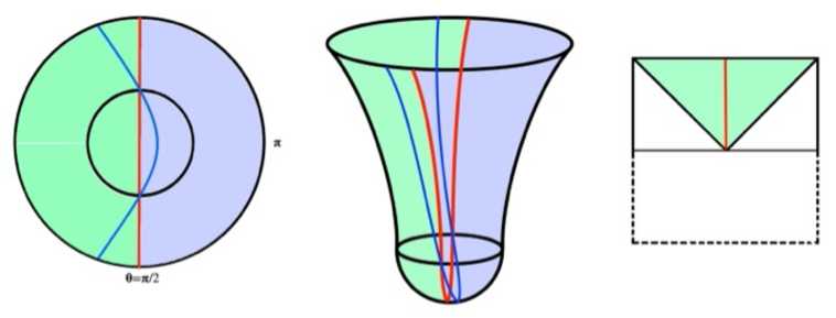
Figure 3: $dS$ no-boundary extremal surfaces in the $t=const$ slice (middle picture; left side is the “top view” from $I^{+}$). The red curve is the extremal surface for maximal boundary subregion, and the blue curve when the subregion is smaller. The green and violet shaded regions are the bulk subregions defined by the time-entanglement or pseudo-entanglement wedges restricted to this $t=const$ slice. The right side figure is the bulk region in the top Lorentzian half in the full $dS$ Penrose diagram, including the $t$ direction: the IR surface lies on the $t=const$ slice which is depicted as the red vertical line.

This leads to a heuristic version of subregion-subregion duality in $dS$, but with some new features relative to the $AdS$ case [66, 67, 68] (and the reviews [16], [69], [70]). For instance in Figure 3, the green shaded region is the bulk subregion or the “time-entanglement wedge” or the “pseudo-entanglement wedge” (restricted to this $t=const$ slice) corresponding to the maximal boundary subregion: we are defining this, just geometrically, as the bulk region bounded by the IR extremal surface and the boundary subregion. Likewise the other maximal (semicircular) subregion gives the complementary violet shaded bulk subregion. In Figure 3, the left and middle pictures pertain to the $t=const$ boundary Euclidean time slice: to obtain the full bulk time-entanglement or pseudo-entanglement wedge, we need to consider the full de Sitter space, including the $t$ direction. This is shown in the right picture: $t=const$ slices are straight lines from $I^{+}$ to the bifurcation point in the top Lorentzian half in the Penrose diagram (the bottom half, with dashed lines, is replaced by the Euclidean hemisphere). The IR surface on the $t=const$ slice is shown as the vertical red line. To define the time-entanglement or pseudo-entanglement wedge, first note that from the bottommost point of the extremal surface (red curve) we can draw out four spacetime regions: the left and right wedges, and the top and bottom wedges. It appears consistent to define the pseudo-entanglement wedge as the top wedge, bounded by the boundary subregion at $I^{+}$. In some sense, this is the domain of dependence of the analog of the $AdS$ homology surface here. This can also be seen to arise from the analytic continuation of the familiar entanglement wedge in $AdS$: given that the analytic continuation (2), (2.1), (8), of the slice and the IR surface amount to a space-time rotation from $AdS$ to $dS$, it is not surprising that the pseudo-entanglement wedge resembles a space-time rotation from the entanglement wedge in $AdS$. Finally, we see that this top (green) wedge is the future universe in the $dS$ static coordinatization.

It is important to note that our discussions here are simply geometric, in analogy with the $AdS$ case, and fuelled by the analytic continuation. Along these lines and using the causality arguments in [68], the bulk pseudo-entanglement wedge for a generic subregion at the future boundary $I^{+}$ would be expected to not lie within its causal wedge which is the past lightcone wedge (the past domain of dependence). The extremal surfaces extend in timelike directions away from the subregion, suggesting causal consistency (see also [22]). One might expect a bulk reconstruction relation of the form $\phi(X)=\int_{I^{+}}d^{d}\sigma G(X,\sigma)O(\sigma)$ with $O(\sigma)$ defined on $I^{+}$ while $\phi(X)$ contains bulk time as well. This is analogous to bulk field expansions $\phi(\sigma,\tau)\sim\int_{{\vec{k}}}G({\vec{k}},\tau,\sigma)\phi_{0}({\vec{k}})$ employed in the late-time Wavefunction in $dS/CFT$ [7], with $\phi_{0}({\vec{k}})$ the future boundary conditions at $I^{+}$. It would be interesting to understand more directly if these heuristic geometric observations and the associated (pseudo-)entanglement wedge reconstruction can be “derived” from analogs in $dS/CFT$ of modular flow, relative entropy, error correction codes and so on [71, 72, 73] (see also the reviews [16], [69], [70]).

Figure 4: $dS$ no-boundary extremal surfaces for disjoint subregions at $I^{+}$ in the $t=const$ slice (static coordinatization): this is the “top view” from $I^{+}$ . These are the red, violet, and blue curves for the three boundary subregions at $I^{+}$. The green, violet and blue shaded regions are the corresponding bulk subregions. The bulk subregions overlap (represented by the different color shadings in the various overlaps; e.g. light blue overlapping with violet leads to darker blue-violet etc).

For these maximal boundary subregions which are disjoint at $I^{+}$, the bulk subregions are also disjoint with no overlap. However now consider Figure 4, depicting the “top view” of three disjoint boundary subregions at $I^{+}$ defined by the arcs bounded by the red, violet and blue curves. The red curve is manifestly seen to be symmetric about the $\theta={\pi\over 2}$ equatorial line: it intersects the $r=l$ inner circle at the $\theta=\pi$ equatorial line (normal to the $\theta={\pi\over 2}$ line). Generic extremal surface curves for other subregions can be drawn likewise by rotating the red curve about the origin of the circles (so they intersect the $r=l$ inner circle at their corresponding ${\tilde{\theta}}={\pi\over 2}$ equatorial line): thus we obtain the violet and blue curves. Now it is clear that the bulk subregions overlap and are not disjoint, even though the corresponding boundary subregions are disjoint. The detailed overlaps can be seen by labelling the green, violet, blue regions as $g,v,b$: then $b+v$ is the blue-violetish overlapping region (colored darker blue-violet) etc, while the central triangular (dark turquoise) region is $g+b+v$. This is the “top view” here (suppressing the analog of the middle image in Figure 3), so it is somewhat distinct from the corresponding picture in $AdS$ of disjoint subregions on a constant time slice.

Figure 5: $dS$ no-boundary extremal surfaces and alternative ways to define bulk subregions (“top view” from $I^{+}$). The bulk subregions for disjoint boundary subregions at $I^{+}$ do not overlap now: however the extremal surface now has a cusp at the no-boundary point (the earlier smooth extremal surface is the blue curve).

There is an alternative way to define bulk subregions geometrically, which leads to the picture in Figure 5. Consider the boundary subregion $[-\theta_{\infty},\theta_{\infty}]$. We construct the extremal surface through the intersections of the maximal (red) extremal surfaces for $[-\theta_{\infty},-\theta_{\infty}+\pi]$ and for $[\theta_{\infty}-\pi,\theta_{\infty}]$: this leads to the two red half surfaces which meet at the origin, i.e. the no-boundary point in the center, but with a cusp since this effectively involves the intersection of two great circles (by comparison the earlier extremal surface is smooth at the no-boundary point). The green bulk subregion is obtained as the region bounded by this cuspy extremal surface and the boundary subregion. Perhaps such cuspy extremal surfaces should be discarded, favouring the earlier smooth ones.

Entirely Lorentzian $dS$, future-past surfaces

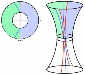
Figure 6: $dS$ future-past extremal surfaces from two copies of no-boundary surfaces (Figure 3). The two copies of no-boundary $dS$ are glued at the $r=l$ plane (removing the bottom hemisphere).

So far we have been describing no-boundary de Sitter extremal surfaces. To discuss future-past surfaces, we first construct entirely Lorentzian de Sitter space by gluing two copies of no-boundary de Sitter space as in Figure 6, with a top Lorentzian half glued onto a bottom Lorentzian half smoothly at the $r=l$ midslice, removing the Euclidean hemispheres in both. We now construct future-past surfaces in entirely Lorentzian de Sitter by gluing two copies of the no-boundary surfaces. For instance, the top timelike part of the (red) IR surface for maximal $I^{+}$ subregion glues smoothly at $r=l$ onto the bottom timelike IR surface anchored at $I^{-}$, to give the entirely timelike IR future-past surface stretching between $I^{\pm}$. The corresponding time-entanglement or pseudo-entanglement wedge comprises the future and past universe, i.e. the rightmost image in Figure 3 (the future universe in the top Lorentzian $dS$) and its past copy. The blue curve shows the future-past extremal surface for non-maximal $I^{\pm}$ subregions. It is worth noting though that reconstructing the entirely Lorentzian bulk appears to involve the two copies in a nontrivial manner (encoding $|\Psi_{dS}|^{2}$ alongwith the area relations (2)).

Finally, it is worth noting that our geometric discussions of the time-entanglement wedge, or pseudo-entanglement wedge, are based on the extremal surfaces on the $t=const$ slice we have been studying, which can be obtained from the analytic continuations of constant time slice RT surfaces in $AdS$. It can be seen that the resulting pictures are somewhat different from those in [22] which discussed analogs of the entanglement wedge based on future-past extremal surfaces on $S^{d}$ equatorial planes in the $dS$ static coordinatization (which would map to equatorial plane slices in $AdS$). These differences are not surprising since the corresponding boundary Euclidean time slices are quite different. The analytic continuation from $AdS$ suggests the slices here as “preferred” as we have stated previously: it would be interesting to understand this better.

2.5 Entropy relations and inequalities

The $AdS$ RT/HRT surface areas are known to strikingly satisfy various entanglement entropy inequalities: we now study $dS$ analogs of some of these using illustrative examples. First, for the IR subregion with $\theta_{\infty}={\pi\over 2}$ , we have $S[A_{IR}]=S[A_{IR}^{C}]$ from (19), i.e. the time-entanglement for the IR subregion and its complement (also an IR subregion) are equal: on geometric grounds it is consistent to take $S[A_{IR}^{C}]=S[A_{IR}]$ for generic $\theta_{\infty}$ subregions and we will use this in what follows. Since the complex-valued areas are somewhat different from the familiar ones in $AdS$, it is unclear if $S[A_{IR}^{C}]=S[A_{IR}]$ implies purity rigorously.

Using the area expressions in $dS_{3}$ (19), we can evaluate formal analogs of mutual information for disjoint boundary subregions. Consider two disjoint adjacent subregions $A,B$, with $|\theta_{\infty}|={\pi\over 4}$ each (so each is a quadrant with spread $2\theta_{\infty}={\pi\over 2}$; see Figure 4): the union subregion $A\cup B$ is the single contiguous $IR$ subregion with $\theta_{\infty}={\pi\over 2}$ (since $A,B$ are adjacent): then, using (19), we have the “mutual time-information” or “mutual pseudo-information”

$$I_{t}[A,B] = S[A]+S[B]-S[A\cup B]$$

$$= 2\Big{(}-i{l\over 2G_{3}}\log{R_{c}\over l}-i{l\over 4G_{3}}\log(\sin^{2}{\pi\over 4})+{\pi l\over 4G_{3}}\Big{)}+i{l\over 2G_{3}}\log{R_{c}\over l}-{\pi l\over 4G_{3}}$$

$$= -i{l\over 2G_{3}}\log{R_{c}\over l}+i{l\over 2G_{3}}\log 2+{\pi l\over 4G_{3}}\,.$$

$$\Rightarrow {\rm Re}\,I_{t}[A,B]>0\,,\qquad{\rm Im}\,I_{t}[A,B]<0\,.$$ (26)

This is also the pattern for adjacent disjoint subregions with other $\theta_{\infty}$ values, as can be seen using the area expression (19), which gives ${\rm Re}I_{t}[A,B]>0,\ {\rm Im}I_{t}[A,B]<0$.

Now let us consider three disjoint adjacent subregions $A,B,C$, each a quadrant with $|\theta_{\infty}|={\pi\over 4}$ each. Together they cover three quadrants of the full circle at $I^{+}$ (schematically picking three of the four quadrants in Figure 4). Recalling [74] in the $AdS$ case, we want to consider the time-entanglement analogs of the inequalities associated with strong subaddivity and tripartite information, using the $dS_{3}$ areas (19). Then $AB\equiv A\cup B$ and $BC\equiv B\cup C$ are maximal subregions with spread $2\theta_{\infty}=\pi$ each (with area given by the IR surface area (10)), while $AC\equiv A\cup C$ comprises antipodal quadrants with the extremal surface comprising an “inner” component with area $S_{A_{+},C_{-}}$ and an “outer” one with area $S_{A_{-},C_{+}}$ (where $A$ and $C$ have endpoints $A_{-},A_{+}$ and $C_{-},C_{+}$). These are equivalent respectively to extremal surfaces for $B$ and its antipodal quadrant. Finally $ABC\equiv A\cup B\cup C$ has area given by its complementary quadrant. Putting these together, we have

$$S_{A}=S_{B}=S_{C}=-i{l\over 2G_{3}}\log{R_{c}\over l}-i{l\over 4G_{3}}\log(\sin^{2}{\pi\over 4})+{\pi l\over 4G_{3}}\equiv S_{\pi/4}\,,\qquad\quad$$

$$S_{AB}=S_{BC}=-i{l\over 2G_{3}}\log{R_{c}\over l}+{\pi l\over 4G_{3}}\equiv S_{\pi/2}\,,\quad\ S_{AC}=S_{\pi/4}+S_{\pi/4}\,,\quad\ S_{ABC}=S_{\pi/4}\,,$$ (27)

with $S_{A}\equiv S[A]$ etc. Using these, we first consider tripartite information which evaluates to

$$I_{3}^{t}[A,B,C] = S_{A}+S_{B}+S_{C}-S_{AB}-S_{BC}-S_{AC}+S_{ABC}$$ (28)

$$= 2S_{\pi/4}-2S_{\pi/2}=i{l\over 2G_{3}}\log 2\qquad\Rightarrow\quad{\rm Im}\,I_{3}^{t}[A,B,C]>0\,.$$

Note that the real parts as well as the imaginary divergent terms cancel completely between the various terms, leaving behind $I_{3}^{t}$ above. This appears unrecognizable in de Sitter per se, but in fact it is consistent via analytic continuation with tripartite information in $AdS$ being negative. Indeed, noting $il\rightarrow-L$, we see that $I_{3}^{t}$ above in $dS$ continues to the negative definite value $I_{3}^{AdS}\sim-{L\over G_{3}}<0$, consistent with [74]. Similar observations can be made for mutual time-information (2.5) and its $AdS$ analytic continuation, where we expect positivity (as can be seen from the leading scaling ${L\over G_{3}}$ of the first term in (2.5) upon continuation).

Likewise the strong subadditivity relations, again recalling [74], become

$$SSB_{1}^{t}=S_{AB}+S_{BC}-S_{ABC}-S_{B}=-i{l\over 2G_{3}}\log 2\,,$$

$$SSB_{2}^{t}=S_{AB}+S_{BC}-S_{A}-S_{C}=-i{l\over 2G_{3}}\log 2\,,$$ (29)

using (2.5). This again is consistent with the known (real) positivity of these inequalities in $AdS$, as can be seen from the analytic continuation $il\rightarrow-L$ and the comments above. As another example, consider the three disjoint boundary subregions $A,B,C$, in Figure 4 (dual to the green, violet, blue bulk subregions), which together make up the full circle ($\theta_{\infty}={\pi\over 3}$ each): then $S_{A}=S_{B}=S_{C}=S_{\pi/3}$, $S_{ABC}=0$ and $S_{AB}=S_{C}$ (since $AB$ is complementary to $C$) etc, so that $I_{3}^{t}=0$. The strong subadditivity relations give $SSB_{1}^{t}=S_{\pi/3}$ and $SSB_{2}^{t}=0$. These can also be seen to be consistent with the $AdS$ entropy positivity relations under the analytic continuation. These thus suggest ${\rm Re}\,SSB_{1,2}^{t}\geq 0,\ \ {\rm Im}\,SSB_{1,2}^{t}\leq 0$.

Finally, consider four disjoint, adjacent subregions $A,B,C,D$, each with $\theta_{\infty}={\pi\over 4}$: each has spread $2\theta_{\infty}={\pi\over 2}$ so together they make up the full circle. Then clearly

$$S[A]+S[B]=S[C]+S[D]\,;\quad S[A\cup B]=S[C\cup D]=S^{IR}\,;\qquad\quad$$ (30)

$A\cup C$ has inner and outer extremal surfaces defined by the complement subregions $B,D$, so

$$I_{t}[A,C]=S[A]+S[C]-S[A\cup C]=S[A]+S[C]-S[B]-S[D]=0\,.$$ (31)

So antipodal dijsoint subregions such as $A,C$ have vanishing mutual time-information (in contrast with (2.5) for adjacent subregions). Note that the top timelike parts of the $A,C$ extremal surfaces are disjoint (meeting at the $r=l$ plane): however the bulk subregions within the hemisphere have overlap so are not disjoint.

Thus the $dS_{3}$ analogs of the entropy relations while being complex-valued and apparently novel in fact intricately encode the known entropy relations satisfied by the $AdS$ RT/HRT areas. From the structure of the areas (8), (9), we expect that these sorts of inequalities will hold in higher dimensional $dS$ as well. It is of course fascinating to ask what these complex-valued entropy inequalities, i.e.  ${\rm Re}\,I_{t}[A,B]\geq 0,\ \ {\rm Im}\,I_{t}[A,B]\leq 0,\ \ {\rm Im}\,I_{3}^{t}[A,B,C]\geq 0$,  etc mean intrinsically in de Sitter space.

2.5.1 Qubit systems and pseudo-entropy/time-entanglement relations

To put in perspective the above de Sitter extremal surface area-entropy relations and inequalities, let us consider time-entanglement/pseudo-entropy in simple quantum mechanical qubit systems, in part recalling the discussions in [44].

Consider a thermofield-double-type initial state $|I\rangle=\sum_{i=1,2}c_{ii}|ii\rangle$ and its time-evolved final state $|F\rangle=\sum_{i}c_{ii}e^{-iE_{ii}t}|ii\rangle$, where the Hamiltonian is $H=E_{ij}|ij\rangle\langle ij|$ with energy eigenvalues $E_{ij}$ for basis states $|ij\rangle$ (and we assume $E_{12}=E_{21}$). Then towards evaluating pseudo-entropy, we note the normalized transition matrix and its partial traces:

$$\rho_{t}={|F\rangle\langle I|\over{\rm Tr}(|F\rangle\langle I|)}={1\over\sum_{j}|c_{jj}|^{2}e^{-iE_{jj}t}}\Big{(}|c_{11}|^{2}e^{-iE_{11}t}|11\rangle\langle 11|+c_{11}c_{22}^{*}e^{-iE_{11}t}|11\rangle\langle 22|$$

$$\qquad\qquad\qquad\qquad\qquad\qquad\qquad\quad+\,c_{11}^{*}c_{22}e^{-iE_{22}t}|22\rangle\langle 11|+|c_{22}|^{2}e^{-iE_{22}t}|22\rangle\langle 22|\Big{)}\,,\qquad\$$ (32)

$$\rho_{t}^{1}={\rm Tr}_{2}\,\rho_{t}={1\over\sum_{j}|c_{jj}|^{2}e^{-iE_{jj}t}}\Big{(}|c_{11}|^{2}e^{-iE_{11}t}|1\rangle\langle 1|+c_{22}|^{2}e^{-iE_{22}t}|2\rangle\langle 2|\Big{)}=\rho_{t}^{2}={\rm Tr}_{1}\,\rho_{t}\,.\ \$$

$\rho_{t}$ can be equivalently regarded [24, 44] as the time evolution operator with projection onto the initial state $|I\rangle$ (and $\rho_{t}^{1},\ \rho_{t}^{2}$, partial traces thereof),

$$\rho_{t}={{\cal U}(t)|I\rangle\langle I|\over{\rm Tr}({\cal U}(t)|I\rangle\langle I|)}\,,\qquad{\cal U}(t)=e^{-iHt}\,,\qquad|F\rangle={\cal U}(t)|I\rangle\,,$$ (33)

Using the normalization $|c_{11}|^{2}+|c_{22}|^{2}=1$ and redefining $|c_{11}|^{2}=x$ recasts this as

$$\rho_{t}^{2}=\rho_{t}^{1}={1\over x+(1-x)e^{i\theta}}\Big{(}x|1\rangle\langle 1|+(1-x)e^{i\theta}|2\rangle\langle 2|\Big{)}\,,\qquad\theta=-(E_{22}-E_{11})t=-\Delta E\,t\,,$$

$$S_{t}^{2}=S_{t}^{1}=-{x\over x+(1-x)e^{i\theta}}\log{x\over x+(1-x)e^{i\theta}}-{(1-x)e^{i\theta}\over x+(1-x)e^{i\theta}}\log{(1-x)e^{i\theta}\over x+(1-x)e^{i\theta}}\,,\qquad$$ (34)

with $S_{t}^{2}=S_{t}^{1}$ the pseudo-entropy of the reduced transition matrix corresponding to states $|I\rangle,|F\rangle$. In the vicinity of $t=0$, we obtain

$$\qquad\qquad\qquad\qquad\qquad S_{t}^{1}(t)\sim S_{t}^{1}(0)+{d\over dt}S_{t}^{1}(0)\,t\equiv S_{0}\,,$$

$$S_{t}^{1}(0)=-x\log x-(1-x)\log(1-x)\,,\qquad{d\over dt}S_{t}^{1}(0)=-i\,\Delta E\,x(1-x)\log{x\over 1-x}\,.\qquad$$ (35)

We see that $S_{t}^{1}(0)$ is the entanglement entropy of the initial state at $t=0$ and is positive definite; however its (pure imaginary) time derivative ${d\over dt}S_{t}^{1}(0)$ switches sign depending on whether $x>{1\over 2}$ or $x<{1\over 2}$ . Thus $S_{0}$ satisfies ${\rm Re}S_{0}>0$ and ${\rm Im}S_{0}\gtrless 0$ for generic $x\neq{1\over 2}$ .

For this 2-qubit system with transition matrix $\rho_{t}$, let us calculate mutual time-information (contrast (2.5). With $\rho_{t}$ regarded as a $2\times 2$-matrix, we have ${\rm det}\,\rho_{t}=0$ so the eigenvalues are $0,1$, and the associated entropy vanishes, i.e. $S_{t}=0$. So in the vicinity of $t=0$, we obtain

$$I_{t}[1,2]=S_{t}^{1}+S_{t}^{2}-S_{t}\sim 2S_{0}\quad\Rightarrow\quad{\rm Re}I_{t}>0\,,\quad{\rm Im}I_{t}\gtrless 0\,.$$ (36)

Thus the imaginary part of mutual time-information has no definite sign for $x\neq{1\over 2}$ (with fixed $\Delta E$). Evaluating $I_{t}$ near $t=0$ illustrates this sharply and explicitly, but it can also be evaluated numerically for general $\theta$ (i.e. $t$) using (2.5.1) verifying the sign non-definiteness. The maximally entangled case $x={1\over 2}$ has  $S_{t}^{2}=S_{t}^{1}=-{1\over 1+e^{i\theta}}\log{1\over 1+e^{i\theta}}-{1\over 1+e^{-i\theta}}\log{1\over 1+e^{-i\theta}}\equiv\alpha+\alpha^{*}$ which is real-valued and positive for all $\theta$ (i.e. $t$) [24, 44].

Now consider a 3-qubit system and a GHZ-type initial state $|I\rangle$ and its time-evolved final state $|F\rangle$, with Hamiltonian $H=\sum E_{ijk}|ijk\rangle$, and normalization $|c_{111}|^{2}+|c_{222}|^{2}=1$,

$$|I\rangle=c_{111}|111\rangle+c_{222}|222\rangle\,,\qquad|F\rangle=c_{111}e^{-iE_{111}t}|111\rangle+c_{222}e^{-iE_{222}t}|222\rangle\,,$$ (37)

Defining $|c_{111}|^{2}\equiv x$, the normalized transition matrix and its various partial traces are

$$\!\!\!\!\rho_{t}^{123}={|F\rangle\langle I|\over{\rm Tr}(|F\rangle\langle I|)}\,,\qquad\qquad\theta=-(E_{22}-E_{11})t=-\Delta E\,t\,,$$

$$\!\!\!\!\rho_{t}^{1}={\rm Tr}_{23}\,\rho_{t}^{123}={1\over x+(1-x)e^{i\theta}}\Big{(}x|1\rangle\langle 1|+(1-x)e^{i\theta}|2\rangle\langle 2|\Big{)}\,,\qquad\rho_{t}^{2}=\rho_{t}^{3}=\rho_{t}^{1}\,,$$ (38)

$$\!\!\!\!\rho_{t}^{12}={\rm Tr}_{3}\,\rho_{t}^{123}={1\over x+(1-x)e^{i\theta}}\Big{(}x|11\rangle\langle 11|+(1-x)e^{i\theta}|22\rangle\langle 22|\Big{)}\,,\qquad\rho_{t}^{23}=\rho_{t}^{13}=\rho_{t}^{12}\,.$$

Operationally it is clear that each of the reduced transition matrices are of the form for the 2-qubit case (2.5.1), so their pseudo-entropies are all of the form $S_{t}^{1}$ there. It can be seen that ${\rm det}\,\rho_{t}^{123}=0$ and the associated pseudo-entropy $S_{t}^{123}$ vanishes (the only eigenvector is $|I\rangle$). Thus finally we evaluate $I_{3}^{t}[1,2,3]=S_{t}^{1}+S_{t}^{2}+S_{t}^{3}-S_{t}^{23}-S_{t}^{13}-S_{t}^{12}+S_{t}^{123}=0$ so the tripartite information for this 3-qubit system vanishes. We can also likewise evaluate the strong subadditivity relations here, and contrast with (2.5): this gives

$$SSB_{1}^{t}=S_{t}^{12}+S_{t}^{23}-S_{t}^{123}-S_{t}^{2}=S_{t}^{1}\,,$$ (39)

while $SSB_{2}^{t}=S_{t}^{12}+S_{t}^{23}-S_{t}^{1}-S_{t}^{3}=0$. Analysing in the vicinity of $t=0$ using (2.5.1) shows

$${\rm Re}\,SSB_{1}^{t}>0\,,\qquad{\rm Im}\,SSB_{2}^{t}\gtrless 0\,;\qquad\quad x\neq{1\over 2}\,,$$ (40)

so the imaginary part of $SSB_{1}^{t}$ switches sign depending on $x\gtrless{1\over 2}$ (for fixed $\Delta E$).

One can also analyse the entropy structures of the time evolution operator as another diagnostic of entanglement-like structures with timelike separations, as in [24, 44]. For the 2-qubit case the normalized time evolution operator is

$$\rho_{t}=\sum_{i,j}{e^{-iE_{ij}t}\over\sum_{kl}e^{-iE_{kl}t}}\,|ij\rangle\langle ij|\,=\,{|11\rangle\langle 11|+e^{i\theta_{1}}|22\rangle\langle 22|+e^{i\theta_{2}}(|12\rangle\langle 12|+|21\rangle\langle 21|)\over 1+e^{i\theta_{1}}+2e^{i\theta_{2}}}$$ (41)

with two arbitrary phases comprising $\theta_{1}\equiv-(E_{22}-E_{11})t\,,\ \theta_{2}\equiv-(E_{12}-E_{11})t$. Taking partial traces gives the reduced time evolution operator for the remaining index,

$$\rho_{t}^{2}=\rho_{t}^{1}={1\over 1+e^{i\theta_{1}}+2e^{i\theta_{2}}}\Big{(}\big{(}1+e^{i\theta_{2}}\big{)}|1\rangle\langle 1|+\big{(}e^{i\theta_{1}}+e^{i\theta_{2}}\big{)}|2\rangle\langle 2|\Big{)}\,.$$ (42)

The associated von Neumann entropies for $\rho_{t}^{1},\rho_{t}^{2}$ and $\rho_{t}$ are [44]

$$S_{t}^{1,2}=-{1+e^{i\theta_{2}}\over 1+e^{i\theta_{1}}+2e^{i\theta_{2}}}\,\log{1+e^{i\theta_{2}}\over 1+e^{i\theta_{1}}+2e^{i\theta_{2}}}\,-\,{e^{i\theta_{1}}+e^{i\theta_{2}}\over 1+e^{i\theta_{1}}+2e^{i\theta_{2}}}\,\log{e^{i\theta_{1}}+e^{i\theta_{2}}\over 1+e^{i\theta_{1}}+2e^{i\theta_{2}}}\ ,$$

$$S_{t}=-{1\over 1+e^{i\theta_{1}}+2e^{i\theta_{2}}}\,\log{1\over 1+e^{i\theta_{1}}+2e^{i\theta_{2}}}\,-\,{e^{i\theta_{1}}\over 1+e^{i\theta_{1}}+2e^{i\theta_{2}}}\,\log{e^{i\theta_{1}}\over 1+e^{i\theta_{1}}+2e^{i\theta_{2}}}\,\qquad$$

$$\qquad\qquad\qquad\ -\,{2e^{i\theta_{2}}\over 1+e^{i\theta_{1}}+2e^{i\theta_{2}}}\,\log{e^{i\theta_{2}}\over 1+e^{i\theta_{1}}+2e^{i\theta_{2}}}\,,$$ (43)

and mutual time-information becomes $I_{t}[1,2]=S_{t}^{1}+S_{t}^{2}-S_{t}=2S_{t}^{1}-S_{t}$ which is complex-valued in general (apart from specific special cases). By numerically evaluating this for generic $\theta_{1,2}$, it can be seen that ${\rm Re}\,I_{t}<0$ while the imaginary part exhibits both signs as $t$ varies (for fixed $E_{ij}$). Evaluating near $t=0$ shows $I_{t}[1,2](0)=0$, ${d\over dt}I_{t}[1,2](0)=0$, with the leading nonzero terms being ${\rm Re}\,I_{t}[1,2]=-{1\over 32}(E_{11}+E_{22}-2E_{12})^{2}t^{2}+\ldots$ and $i{\rm Im}\,I_{t}[1,2]=i{1\over 1536}(E_{22}-E_{11})^{2}(E_{11}+E_{22}-2E_{12})t^{5}+\ldots$, verifying the sign-nondefiniteness of the imaginary part.

The above qubit examples are quite simple in structure but serve to explicitly illustrate the behaviour of pseudo-entropy/time-entanglement relations and inequalities. More complicated qubit examples quickly become very intricate in their entropy structures. It is clear that these simple qubit examples in quantum mechanics are quite different in their pseudo-entropy inequalities behaviour compared with the properties we saw for de Sitter extremal surfaces earlier. In some ways this is not surprising: it reflects the striking differences found in [74] with regard to entropy inequalities for the $AdS$ RT surface areas and entanglement entropies in theories with gravity duals, in comparison with qubit systems and generic CFTs. The (generically) complex-valued nature of pseudo-entropies makes the entropy relations and inequalities more intricate overall: it would be interesting to understand the underlying organizational principles here, especially in nonunitary theories with $dS$-like gravity duals.

2.6 Antipodal observers at $I^{+}$ to codim-2 surfaces

So far we have been discussing codim-2 extremal surfaces, which appear natural from the point of view of Euclidean time slices of the dual boundary theory. From the bulk point of view, one might imagine asking for natural subregions at $I^{+}$ being codim-0, i.e. smaller regions of the $S^{d}$ at $I^{+}$ (in $dS_{d+1}$). For instance, for $dS_{3}$ with the $S^{2}$ at $I^{+}$, this would lead to cap-like subregions on the $S^{2}$ which lead to maximal subregions being hemispheres. These would lead to codim-1 surfaces anchored at the boundary of these subregions.

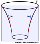
Figure 7: Antipodal observers $O_{1}$ and $O_{2}$ at $I^{+}$ in $dS$, and the boundary Euclidean time slice they define. This gives rise to maximal subregions with corresponding IR extremal surfaces.

Instead consider two antipodal observers at $I^{+}$, not in causal contact, and unable to communicate with each other. For simplicity consider them to be stationary, so they are represented by timelike trajectories parametrized by global $dS$ time $\tau$ at the North and South Poles, with all other angular coordinates fixed. These antipodal observers are “maximally separated”, whereas two generic observers are not. While either observer (at either North or South Pole) can only access information pertaining to half the space, the two antipodal observers together provide a complete description of the entire de Sitter space (these are best regarded as metaobservers in the sense of [6]).

These two antipodal points define a plane normal to $I^{+}$: this is a natural “vertical” bulk slice which is essentially a boundary Euclidean time slice corresponding to an equatorial plane of the $S^{d-1}$. Any two antipodal observers define such equatorial boundary Euclidean time slices which are all equivalent: so there is a continuum $S^{d-1}$ of such antipodal observers. Note also that from (2.1), the $t=const$ slice in the $dS$ static coordinatization defines the same boundary Euclidean time slice as a generic equatorial plane in global $dS$ obtained from two antipodal observers.

Now these two observers will draw RT/HRT surfaces going into the time direction (no single local patch suffices): their areas are perhaps best regarded as meta-observables as described in [6]. These now are future-past or no-boundary extremal surfaces, with all their properties: in particular the no-boundary extremal surface stretching out from one observer only returns to the other observer (after turning around in the bottom Euclidean hemisphere). The maximal subregions here are $S^{d-1}$ hemispheres so the extremal surface is anchored on the $S^{d-2}$ boundary and dips into time, i.e. wrapping $S^{d-2}\times\tau$ which gives a codim-2 surface.

In the static coordinatization with boundary topology $R_{t}\times S^{d-1}$, the analytic continuation lands on the $t=const$ slice as we have seen, from (2.1): this defines “preferred” observers whose extremal surfaces wrap the $S^{d-2}$ boundary of the $S^{d-1}$ subregions. For maximal subregions ($S^{d-1}$ hemispheres) the IR extremal surfaces wrap $S^{d-2}\times\tau$ and are maximal: calculationally these are identical to those in the equatorial plane global slicing above.

It would be instructive to develop the point of view of these antipodal (meta)observers further, possibly connecting the description here of codim-2 extremal surfaces (which are akin to metaobservables at the future boundary) with [75], as well as [31] more directly.

3 No-boundary $dS$: Lewkowycz-Maldacena heuristically to pseudo-entropy

In this section, we will discuss how the analytic continuation from $AdS$ to $dS$ maps the Lewkowycz-Maldacena replica argument [54] deriving the $AdS$ RT surfaces to a corresponding heuristic version of the replica argument in $dS$. Our discussion is somewhat formal based mainly on the analytic continuation. While a Lewkowycz-Maldacena argument for pseudo-entropy appears in [33] in the $AdS$ context, the arguments here are specific to de Sitter which has several new features. Most notably the $dS/CFT$ dictionary $Z_{CFT}=\Psi_{dS}$ [7] implies that a replica on the boundary partition function (for boundary entanglement entropy) amounts to a replica on the bulk $dS$ Wavefunction (a single ket, rather than a density matrix), so it is best interpreted as giving rise to bulk pseudo-entropy, which is the main takeaway. Quantitatively, this recovers the IR no-boundary $dS$ areas in (1.1) from the areas of appropriate codim-2 cosmic branes, as we will see.

First we note that under the analytic continuation from global $AdS$ to $dS$, the bulk $AdS$ partition function continues to the bulk $dS$ Wavefunction of the Universe $\Psi_{dS}$ see e.g. [7], [64], [65]). This Hartle-Hawking Wavefunction [76], semiclassically, can be represented by a gravitational path integral

$$\Psi_{dS}[h_{ij},\phi_{0}]=\int_{nb}^{I^{+}}Dg\,D\phi\ e^{iS[g,\phi]}$$ (44)

obtained by summing over all $(d+1)$-manifolds with $h_{ij}$ as the metric on the spatial slice at the future boundary $I^{+}$ (and $\phi_{0}$ are final source boundary conditions for matter fields $\phi$). There is no time that appears in this representation of $\Psi_{dS}$: time implicitly enters in the sum over bulk spacetime histories. This Wavefunction $\Psi_{dS}[h_{ij}]$ can be regarded as the amplitude for creating the universe $M[h_{ij}]$ with these final boundary conditions from “nothing”, i.e. satisfying the Hartle-Hawking no-boundary condition (which is also imposed on the matter fields $\phi$). Then it is reasonable to regard this Wavefunction $\Psi[h_{ij}]$ as the transition amplitude $\rho_{t}$ for “nothing”$\rightarrow$ $M[h_{ij}]$. No-boundary de Sitter space arises, as we have seen in e.g. (2), by gluing the top Lorentzian part to the bottom Euclidean hemisphere at the $r=l$ midplane. Semiclassically, the Wavefunction is given by the action as

$$\Psi_{dS}\ \sim\ e^{iS^{(r>l)}}\,e^{S_{E}^{(r<l)}}$$ (45)

with the top Lorentzian part (with real $S^{(r>l)}$) being a pure phase while the bottom Euclidean hemisphere has real action. Global $dS$ in (3) continues to the bottom Euclidean hemisphere as $ds^{2}=l^{2}d\tau_{E}^{2}+l^{2}\cos^{2}\tau_{E}\,d\Omega_{d}^{2}$ with $\tau=i\tau_{E}$, $0\leq\tau_{E}\leq{\pi\over 2}$ : then the Lorentzian $iS_{cl}$ continues to the Euclidean gravity action  $S_{E}^{(r<l)}=-\int_{{}_{{}_{nbp}}}\sqrt{g}\,(R-2\Lambda)$  in the hemisphere, giving  ${1\over 2}\,{l^{4}V_{S^{4}}\over 16\pi G_{4}}\,{6\over l^{2}}={\pi l^{2}\over 2G_{4}}$  for $dS_{4}$ (the no-boundary point is $\tau_{E}={\pi\over 2}$ here).  So the probability for creating $dS$ from no-boundary nothingness is the Hartle-Hawking factor $|\Psi_{dS}|^{2}=e^{dS.entropy}$ from $S_{E}^{(r<l)}$  [76] (see also e.g. [77, 78], as well as [79]). Further, see [65] for $dS_{2}$, [25] for the $dS_{3}$ case, [23, 24] for related discussions in the context of the no-boundary extremal surface areas, and also the recent [80] in the context of the Wheeler-de Witt equation.

We are attempting to closely mimic some of the $AdS$ arguments in [55] (see also [56], [57]) extending [54], as reviewed in [16] and [59] in extending to the $dS$ case here. Since the analytic continuation from $AdS$ to $dS$ maps $Z_{bulk}\rightarrow\Psi_{dS}$, the replica construction of Lewkowycz-Maldacena [54] in $AdS$ is now a formulation on the Wavefunction, restricted to the boundary Euclidean time slice (mapped from the constant time slice in $AdS$ where the subregion is defined). The associated entropy is then the entropy of the corresponding transition matrix, i.e. the time-entanglement or pseudo-entropy.

Let us first do a quick review of the $AdS$ case: here, we are considering a boundary subregion on a constant time slice. The subregion boundary is then codim-2 so the bulk extremal surface anchored on it is also codim-2 in the bulk. The replica space is an $n$-fold branched cover over the boundary, branched over the subregion boundary on the constant time slice (which thus makes the subregion boundary codim-2). The ${\mathbb{Z}}_{n}$ replica symmetry permutes the $n$ boundary copies. The boundary replica space $M_{n}$ extends into a smooth bulk replica space ${\cal B}_{n}$ which is to be regarded as a smooth covering space wth replica boundary conditions for gluing the $n$ copies (cyclically). If we now consider the quotient ${\tilde{\cal B}_{n}}$ of the bulk space by the ${\mathbb{Z}}_{n}$ replica symmetry (so its boundary is $\partial{\tilde{\cal B}_{n}}=M_{n}/{\mathbb{Z}}_{n}=M_{1}$, the original boundary space), then we encounter conical (orbifold) singularities corresponding to ${\mathbb{Z}}_{n}$ fixed points in the bulk for $n\neq 1$. These curvature singularities are a reflection of the fact that the bulk quotient space is a solution to the bulk Einstein equations only in the presence of a source with nontrivial backreaction. Since the fixed points extend out from the subregion boundary, the required source in question is a codim-2 (cosmic) brane with tension ${n-1\over n}{1\over 4G}$ (giving deficit angle $2\pi-{2\pi\over n}$). The replica quotient space ${\tilde{\cal B}_{n}}$ comprises $n$ copies which are locally the same as a single copy, except for the fixed point singularity: this is smoothed out by the codim-2 cosmic (spacelike) brane source which has area $A$ (wrapping all the transverse directions). Thus the smooth action $I_{n}$ can be written as

$$I_{n}=nI_{1}+I_{brane}=nI_{1}+{n-1\over n}{A\over 4G}\ \ \xrightarrow{\,n=1+\epsilon\,}\ \ (1+\epsilon)I_{1}+\epsilon\,{A\over 4G}\,,$$ (46)

where we have written $n=1+\epsilon$ near $n=1$. In the limit when $n\rightarrow 1$, the cosmic brane becomes a tensionless probe localized on the bulk RT/HRT surface. Defining the bulk partition function $Z_{n}\equiv Z[{\tilde{\cal B}_{n}}]$ on the replica quotient space ${\tilde{\cal B}_{n}}$, the entropy via replica is obtained as

$$S=-\lim_{n\rightarrow 1}n\partial_{n}(\log Z_{n}-n\log Z_{1})=\lim_{n\rightarrow 1}(1-n\partial_{n})\log Z_{n}=-\lim_{n\rightarrow 1}(1-n\partial_{n})I_{n}$$ (47)

in the semiclassical approximation where $Z_{n}\sim e^{-I_{n}}$, with $I_{n}$ the action. Also, $Z_{n}={\rm tr}\,\rho^{n}$, and $Z_{1}^{n}$ ensures that the entropy pertains to the correct normalization ${\rm tr}\,\rho=1$. Thus as $n\rightarrow 1$ (i.e. $\epsilon\rightarrow 0$), we obtain $S={A\over 4G}$ which is the area of the extremal RT/HRT entangling surface.

We can obtain a heuristic understanding of the replica formulation of the entropy of the Wavefunction by following through (for simplicity) the analytic continuation (8) for the IR extremal surface in $dS$ on the $t=const$ slice, i.e. for the maximal subregion at $I^{+}$ (with area (9) for $dS_{4}$ and (10) for $dS_{3}$). In this case, we are inserting twist operators at the $\theta=\pm{\pi\over 2}$ endpoints of the (hemispherical) maximal subregion at $I^{+}$ on the $t=const$ slice (Figure 2) and then constructing $n$ copies of the Wavefunction $\Psi$ appropriately gluing the $n$ copies cyclically with replica boundary conditions. Under the analytic continuation we have

$$Z_{bulk}\sim e^{-I_{bulk}}\ \ \longrightarrow\ \ \Psi_{dS}\sim e^{iS_{cl}}$$ (48)

for a single copy. In the replica case with $n$ copies, we expect

$${Z_{n}\over Z_{1}^{n}}\ \ \longrightarrow\ \ {\Psi_{n}\over\Psi_{1}^{n}}\,.$$ (49)

$\Psi_{n}$ is the Wavefunction on the quotient bulk replica space with nontrivial replica boundary conditions on the future boundary (and $\Psi_{1}$ for a single copy).  Semiclassically, we have

$$Z_{n}\sim e^{-I_{n}}\longrightarrow\Psi_{n}\sim e^{iS_{n}}\,;\qquad\quad-I_{n}\ \rightarrow\ iS_{n}=iS_{n}^{(r>l)}+S_{E}^{(r<l)}\,,$$ (50)

where, under (2), the semiclassical $AdS$ action maps to Lorentzian $dS$ in the top Lorentzian $r>l$ part (with pure imaginary $iS_{n}$) and the bottom Euclidean hemisphere for $r<l$ (with real $S_{E}$). The codim-2 brane source for $n\neq 1$ has nontrivial (part Euclidean, part Lorentzian) time evolution: in the $n\rightarrow 1$ limit it satisfies the no-boundary condition and wraps the will-be no-boundary $dS$ extremal surface. Now continuing from above gives $-I_{brane}\rightarrow{1-n\over n}{A_{brane}\over 4G}$ so we obtain the area in $dS$ (with $n\rightarrow 1$) as

$$S_{t}=\lim_{n\rightarrow 1}(1-n\partial_{n})\log\Psi_{n}=\lim_{n\rightarrow 1}(1-n\partial_{n})\,{1-n\over n}\,{A_{brane}\over 4G}={A^{dS}_{brane}\over 4G}\,.$$ (51)

This is not a spacelike brane here localized on a spacelike RT/HRT surface but a time-evolving brane localized on the part Euclidean, part Lorentzian no-boundary $dS$ extremal surface. The area is complex (with (9), (10), for $dS_{4}$ and $dS_{3}$ respectively). This is a replica formulation of the entropy of the Wavefunction (restricted to this boundary Euclidean slice): this is not hermitian, unlike an ordinary density matrix. It is thus best interpreted as time-entanglement or pseudo-entropy, rather than ordinary spatial entanglement entropy.

It is reasonable that this entropy is complex-valued, with the top Lorentzian timelike part being pure imaginary in particular. In the Lewkowycz-Maldacena replica formulation, the entropy arises as the area of the codim-2 brane created from nothing. The amplitude for this process would be divergent if the Lorentzian part (which goes all the way to late times) were real: as it stands, the timelike parts give pure phases which cancel in the probability. We obtain a finite value since the real part of this entropy is bounded, arising as it does from the brane wrapping the Euclidean hemisphere which has a maximal size (set by de Sitter entropy).

The above arguments are of course consistent with the entropy here being the analog of the entanglement entropy in the nonunitary Euclidean CFT dual to $dS$. Since $\Psi_{dS}=Z_{CFT}$ via $dS/CFT$ this amounts to a replica formulation on $Z_{CFT}$ which is an analytic continuation of $Z_{CFT}=Z_{bulk}^{AdS}$. The analytic continuations (9), (10), of the extremal surface areas in $dS_{4},\ dS_{3}$, respectively can be seen to be the analytic continuations of the entanglement entropy for the relevant maximal subregions in $AdS$ (with sphere boundary). This is broadly consistent with the early discussions on holographic entanglement in $dS/CFT$ by analytic continuations [17, 18], [19], and with appropriate analytic continuations of entanglement entropy in 2-dim CFT [81, 82, 83].

It is to be noted that the arguments above leading to (51) are obtained via analytic continuation from $AdS$. As discussed above, these appear reasonable for the perspective here, give the expected no-boundary $dS$ extremal surface areas and are consistent with expectations of the boundary nonunitary CFT. Assumptions implicit here are that $I_{n}$ is indeed the dominant saddle when analysed directly in the de Sitter case and is well-behaved for the purposes here: it would be instructive to analyse this more explicitly.

In addition, it would be nice to understand if there are alternative ways to formulate the Lewkowycz-Maldacena replica arguments, without relying on the analytic continuation. It is then conceivable that one ends up with not one copy of the Wavefunction but with both a ket and a bra, appropriately glued in some appropriate Schwinger-Keldysh replica path integral. It might then (naively) seem that such a formulation would be analogous to a replica on $Z_{CFT}^{*}Z_{CFT}$ and thus be manifestly positive with no timelike component, unlike the above (see [62] for some related comments in the context of ghost CFT replicas and $dS/CFT$).

4 On future-past entangled states and time-evolution

We now attempt to draw analogies with the arguments in [84], [85], to understand certain aspects of future-past entangled states and connectedness of time evolution and thereby emergence of time. We will mostly focus on ordinary quantum mechanics here.

It was argued in [21, 22], that future-past de Sitter extremal surfaces stretching between $I^{\pm}$ suggest future-past entanglement between two copies of the dual Euclidean CFT in thermofield-double type entangled states, in analogy with the eternal $AdS$ black hole [28]. Certain properties of such states were further studied in [24]. With this in mind, consider doubling the Hilbert space ${\cal H}$ of some quantum system, described by Hamiltonian eigenstates $|I\rangle$ with energies $E_{I}$. The past copy, say at $t=0$, will be denoted by ${\cal H}_{P}$ and the future copy at say $t=T$, is ${\cal H}_{F}$, and is essentially isomorphic to ${\cal H}_{P}$, with the isomorphism map being the time evolution operator ${\cal U}(t)$. The isomorphism is characterized by the standard time evolution of the Hamiltonian eigenstates, i.e.

$${\cal U}(t)=e^{-iHt}\,:\quad|I\rangle_{F}=e^{-iE_{I}T}|I\rangle_{P}$$ (52)

Then generic states in ${\cal H}^{(1)}\times{\cal H}^{(2)}={\cal H}_{F}\times{\cal H}_{P}$ are

$$|\Psi_{g}\rangle_{FP}=\sum_{I,J}c_{IJ}|I\rangle_{F}^{(1)}|J\rangle_{P}^{(2)}=\sum_{I,J}c_{IJ}e^{-iE_{I}T}|I\rangle_{P}^{(1)}|J\rangle_{P}^{(2)}\equiv|\Psi_{g}\rangle_{PP}$$ (53)

These sorts of states involve timelike separations between the states from the $F$ and $P$ copies, which translates to time evolution phases when written in terms of corresponding states in ${\cal H}_{P}^{(1)}\times{\cal H}_{P}^{(2)}$. There are a few noteworthy points here, in considering such a doubling of the Hilbert space.

Firstly, ${\cal H}_{F}\times{\cal H}_{P}$ (motivated by future-past $dS$ surfaces is somewhat different qualitatively from factorizing a Hilbert space as ${\cal H}={\cal H}_{L}\times{\cal H}_{R}$ (as in the $CFT_{L}\times CFT_{R}$ dual to the eternal $AdS$ black hole): in that case there is no causal connection between the components ${\cal H}_{L}$ and ${\cal H}_{R}$, which are independent. In the current case ${\cal H}_{F}$ is the time evolution of ${\cal H}_{P}$, i.e. the time evolution operator acts as the isomorphism. So a state $|\Psi\rangle_{FP}$ is isomorphic to a corresponding state $|\Psi\rangle_{FF}$. Since the time evolution phases cancel, the state $|\Psi\rangle_{FP}$ is future-past entangled if the corresponding state $|\Psi\rangle_{FF}$ is entangled in the ordinary sense on the (constant) late time slice $F$.

To elaborate, consider a factorized future-past state (53) and the partial trace over the past copy of the corresponding future-past density matrix $\rho_{fp}$:

$$|\Psi\rangle_{fp}=|\psi_{F}\rangle^{(1)}|\psi_{P}\rangle^{(2)}={\cal U}(t)|\psi_{P}^{\prime}\rangle^{(1)}|\psi_{P}\rangle^{(2)}\quad\rightarrow\quad{\rm Tr}_{P}\,\big{(}|\Psi\rangle_{fp}\langle\Psi|_{fp}\big{)}=|\psi_{F}\rangle^{(1)}\langle\psi_{F}|^{(1)}$$ (54)

which is pure at the future time slice, with zero entropy. Note also that the time evolution operator ${\cal U}(t)$ has disappeared in the future-past density matrix. This calculation thus does not care whether $|\psi_{F}\rangle$ and $|\psi_{P}\rangle$ belong in the same Hilbert space: the state effectively is $|\psi_{F}\rangle^{(1)}|\psi_{P}\rangle^{(2)}$ with two disconnected spaces $1,2$.

On the other hand, a non-factorizable future-past state such as that in (53) has generic nonzero coefficients $c_{IJ}$ giving the trace over the past copy of the future-past density matrix $\rho_{fp}=|\Psi\rangle_{FP}\langle\Psi|_{FP}$ as

$${\rm Tr}_{P}\,\big{(}|\Psi\rangle_{FP}\langle\Psi|_{FP}\big{)} = {\rm Tr}_{P}\,\sum_{IJ,KL}c_{IJ}c^{*}_{KL}|I\rangle_{F}^{(1)}|J\rangle_{P}^{(2)}\langle K|_{F}^{(1)}\langle L|_{P}^{(2)}$$ (55)

$$= \sum_{IJ,KL}\delta_{JL}c_{IJ}c^{*}_{KL}|I\rangle_{F}^{(1)}\langle K|_{F}^{(1)}=\sum_{I,K}c_{IJ}c^{*}_{KJ}e^{-iE_{I}T}e^{iE_{K}T}|I\rangle_{P}^{(1)}\langle K|_{P}^{(1)}\qquad$$

The form in terms of the $F$ copies alone is seen to be entirely positive: this is a mixed state with nonzero (ordinary) entanglement entropy at the future time-slice $T$ if the future-past state is non-factorizable, i.e. entangled.

The time evolution operator can be obtained as a reduced transition matrix with thermofield double type states using basis states $|i\rangle$ as below (with the normalization done later):

$$\qquad|\psi_{I}\rangle=\sum_{i=1}^{N}|i\rangle_{P}^{(1)}|i\rangle_{P}^{(2)}\,,\qquad|\psi_{FP}\rangle=\sum_{i=1}^{N}|i\rangle_{F}^{(1)}|i\rangle_{P}^{(2)}=\sum_{i=1}^{N}e^{-iE_{i}t}|i\rangle_{P}^{(1)}|i\rangle_{P}^{(2)}\,,$$

$${\cal U}(t)=\sum_{i=1}^{N}e^{-iE_{i}t}|i\rangle_{P}\langle i|_{P}=\sum_{i=1}^{N}|i\rangle_{F}\langle i|_{P}$$

$$\qquad\qquad\qquad\qquad={\rm Tr}_{2}\,\big{(}|\psi_{FP}\rangle\langle\psi_{I}|\big{)}=\sum_{i,j}\delta_{ij}^{(2)}\big{(}|i\rangle_{F}^{(1)}|i\rangle_{P}^{(2)}\,\langle j|_{P}^{(1)}\langle j|_{P}^{(2)}\big{)}\,.$$ (56)

This is distinct in detail from the way the time evolution operator was obtained by the doubled Hilbert space states in [23], [44]. In particular here $|\psi_{FP}\rangle\in{\cal H}_{F}\times{\cal H}_{P}$ for nonzero $t$ so it is a future-past entangled state. The time evolution operator acts as the map from the past space to the future one which is not independent from the past one. Thus the existence of the time evolution operator appears to be tantamount to the existence of future-past entangled states of the form $|\psi_{FP}\rangle$. To elaborate, the time evolution operator implies connectedness of the future and past slices by time evolution: the existence of future-past entangled states is thus equivalent to this time-connectedness.

It is worth noting two aspects of the above (in part elaborating on the corresponding discussions in [24]). One is the fact that the time evolution operator itself can be obtained by partial trace over the second copy in a doubled Hilbert space construction involving future-past entangled states $|\psi_{FP}\rangle$ as in (4). This contains non-positive structures, in particular the time evolution phases, and arises from just a single copy of $|\psi_{FP}\rangle$ (in some sense, this dovetails with the comments at the end of the previous section, sec. 3, on Lewkowycz-Maldacena for a single copy of the $dS$ Wavefunction giving rise to pseudo-entropy). The other pertains to constructing a density matrix from two copies of $|\psi_{FP}\rangle$, as in (55): this leads to entirely positive structures. It would be interesting to understand the interplay between these two aspects more elaborately.

In the bulk de Sitter space, the future-past surfaces connecting the past and future time slices are essentially the extremal time evolution trajectories of codim-2 branes: so their existence is tantamount to time evolution connecting the future and past slices in the same physical spacetime. One might ask if these future-past surfaces “break” and disconnect: it would appear that this would not occur except if the spacetime itself “tears” (for instance, a sufficiently singular perturbation from $I^{-}$ might create a Big-Crunch singularity and thereby destroy $I^{+}$, so timelike trajectories end at the singularity). Our discussions here have been for small fluctuations about de Sitter so the future-past surfaces appear to always exist. As an aside, Schwarzschild de Sitter black holes, regarded as other possible endpoints to strong perturbations, also admit similar future-past surfaces stretching between $I^{\pm}$ and dipping further in towards the black hole [86] (but $dS/CFT$ interpretations are unclear for $SdS$).

5 Discussion

We have developed further the investigations in [24] on de Sitter space, extremal surfaces and time entanglement. We obtain the no-boundary de Sitter extremal surface areas as certain analytic continuations from $AdS$ (in part overlapping with [23]) while also amounting to space-time rotations geometrically. This is most easily seen (sec. 2.1) for the IR extremal surface for maximal subregions in any $dS_{d+1}$ and more generally in greater detail for $dS_{3}$ (sec. 2.2). The structure of the extremal surfaces also suggests a geometric picture of the time-entanglement or pseudo-entanglement wedge (sec. 2.4). In sec. 2.6, we have given certain simple arguments connecting two antipodal (meta)observers and codim-2 surfaces. The analytic continuation suggests a heuristic Lewkowycz-Maldacena formulation of the $dS$ extremal surface areas via analytic continuation sec. 3: in the bulk, this is now a replica formulation on the Wavefunction (single copy) which suggests interpretation as pseudo-entropy. Finally we also discuss aspects of future-past thermofield states and time evolution in quantum mechanics in sec. 4, suggesting close relations between the time evolution operator and future-past entangled states. Several of the discussions here are suggestive rather than conclusive: we hope to understand them more firmly over time.

In sec. 2.5, we studied de Sitter analogs of some of the well-known entropy relations satisfied by RT/HRT surfaces in $AdS$, specifically mutual information, tripartite information and strong subadditivity, focussing on the detailed area expressions in $dS_{3}$ for generic subregions. The complex-valued areas imply complex-valued entropy inequalities,  ${\rm Re}\,I_{t}[A,B]\geq 0,\ \ {\rm Im}\,I_{t}[A,B]\leq 0,\ \ {\rm Im}\,I_{3}^{t}[A,B,C]\geq 0$ etc, which appear novel in themselves (and also show interesting differences compared with pseudo-entropy in qubit systems). However as we saw via the $AdS$ analytic continuation, these in fact intricately encode the known positivity properties in $AdS$ [74]. It is fascinating to ask how the entropy relations are organized intrinsically in $dS$: perhaps these encode interesting properties of both de Sitter space and of pseudo-entropy for (nonunitary) theories with $dS$-like holographic duals.

It is important to note that our discussions in sec. 2.4 for the time-entanglement or pseudo-entanglement wedge in no-boundary de Sitter (resembling a space-time rotation from the entanglement wedge in $AdS$) are simply geometric, and based on the analytic continuation. It would be fascinating to “derive” these heuristic geometric observations more directly from analogs in $dS/CFT$ of modular flow, relative entropy, error correction codes and so on [71, 72, 73]. It would appear that this would amount to a detailed understanding of how entanglement wedge reconstruction works in de Sitter. In this regard, we note that the central dictionary $Z_{CFT}=\Psi_{dS}$ (naively) suggests the bulk-boundary relations are perhaps more intricate here, with nontrivial entry of $|\Psi_{dS}|^{2}$ and the area relations (2) in the way bulk subregions are encoded from boundary data at $I^{+}$. It would be interesting to develop our discussions here incorporating these, and to possibly usefully adapt the discussions in [87] to the de Sitter case. We hope to address these and related issues in the future.

Acknowledgements:  It is a pleasure to thank Philip Argyres, Sumit Das, Daniel Harlow, Veronika Hubeny, Juan Maldacena, Alex Maloney, Shiraz Minwalla, Rob Myers, Suvrat Raju, Mukund Rangamani, Al Shapere, Andy Strominger and Mark van Raamsdonk for helpful discussions, and also Mukund Rangamani and Hitesh Saini for comments on a draft. I thank the Organizers of Strings 2023, Perimeter Institute, and the String Group, U.Kentucky, for hospitality while this work was in progress. This work is partially supported by a grant to CMI from the Infosys Foundation.

References

- [1]
- [2] J. M. Maldacena, “The large N limit of superconformal field theories and supergravity,” Adv. Theor. Math. Phys. 2, 231 (1998) [Int. J. Theor. Phys. 38, 1113 (1999)] [arXiv:hep-th/9711200].
- [3] S. S. Gubser, I. R. Klebanov and A. M. Polyakov, “Gauge theory correlators from non-critical string theory,” Phys. Lett. B 428, 105 (1998) [arXiv:hep-th/9802109].
- [4] E. Witten, “Anti-de Sitter space and holography,” Adv. Theor. Math. Phys. 2, 253 (1998) [arXiv:hep-th/9802150].
- [5] A. Strominger, “The dS / CFT correspondence,” JHEP 0110, 034 (2001) [hep-th/0106113].
- [6] E. Witten, “Quantum gravity in de Sitter space,” [hep-th/0106109].
- [7] J. M. Maldacena, “Non-Gaussian features of primordial fluctuations in single field inflationary models,” JHEP 0305, 013 (2003), [astro-ph/0210603].
- [8] D. Anninos, T. Hartman and A. Strominger, “Higher Spin Realization of the dS/CFT Correspondence,” Class. Quant. Grav. 34, no. 1, 015009 (2017) doi:10.1088/1361-6382/34/1/015009 [arXiv:1108.5735 [hep-th]].
- [9] M. Spradlin, A. Strominger and A. Volovich, “Les Houches lectures on de Sitter space,” hep-th/0110007.
- [10] D. Anninos, “De Sitter Musings,” Int. J. Mod. Phys. A 27, 1230013 (2012) doi:10.1142/S0217751X1230013X [arXiv:1205.3855 [hep-th]].
- [11] D. A. Galante, “Modave lectures on de Sitter space & holography,” PoS Modave2022, 003 (2023) doi:10.22323/1.435.0003 [arXiv:2306.10141 [hep-th]].
- [12] G. W. Gibbons and S. W. Hawking, “Cosmological Event Horizons, Thermodynamics, and Particle Creation,” Phys. Rev. D 15, 2738 (1977). doi:10.1103/PhysRevD.15.2738
- [13] S. Ryu and T. Takayanagi, “Holographic derivation of entanglement entropy from AdS/CFT,” Phys. Rev. Lett. 96, 181602 (2006) [hep-th/0603001].
- [14] S. Ryu and T. Takayanagi, “Aspects of Holographic Entanglement Entropy,” JHEP 0608, 045 (2006) [hep-th/0605073].
- [15] V. E. Hubeny, M. Rangamani and T. Takayanagi, “A Covariant holographic entanglement entropy proposal,” JHEP 0707 (2007) 062 [arXiv:0705.0016 [hep-th]].
- [16] M. Rangamani and T. Takayanagi, “Holographic Entanglement Entropy,” Lect. Notes Phys. 931, pp.1-246 (2017) Springer, 2017, doi:10.1007/978-3-319-52573-0 [arXiv:1609.01287 [hep-th]].
- [17] K. Narayan, “de Sitter extremal surfaces,” Phys. Rev. D 91, no. 12, 126011 (2015) [arXiv:1501.03019 [hep-th]].
- [18] K. Narayan, “de Sitter space and extremal surfaces for spheres,” Phys. Lett. B 753, 308 (2016) [arXiv:1504.07430 [hep-th]].
- [19] Y. Sato, “Comments on Entanglement Entropy in the dS/CFT Correspondence,” Phys. Rev. D 91, no. 8, 086009 (2015) [arXiv:1501.04903 [hep-th]].
- [20] M. Miyaji and T. Takayanagi, “Surface/State Correspondence as a Generalized Holography,” PTEP 2015, no. 7, 073B03 (2015) doi:10.1093/ptep/ptv089 [arXiv:1503.03542 [hep-th]].
- [21] K. Narayan, “On extremal surfaces and de Sitter entropy,” Phys. Lett. B 779, 214 (2018) [arXiv:1711.01107 [hep-th]].
- [22] K. Narayan, “de Sitter future-past extremal surfaces and the entanglement wedge,” Phys. Rev. D 101, no.8, 086014 (2020) doi:10.1103/PhysRevD.101.086014 [arXiv:2002.11950 [hep-th]].
- [23] K. Doi, J. Harper, A. Mollabashi, T. Takayanagi and Y. Taki, “Pseudoentropy in dS/CFT and Timelike Entanglement Entropy,” Phys. Rev. Lett. 130, no.3, 031601 (2023) doi:10.1103/PhysRevLett.130.031601 [arXiv:2210.09457 [hep-th]].
- [24] K. Narayan, “de Sitter space, extremal surfaces, and time entanglement,” Phys. Rev. D 107, no.12, 126004 (2023) doi:10.1103/PhysRevD.107.126004 [arXiv:2210.12963 [hep-th]].
- [25] Y. Hikida, T. Nishioka, T. Takayanagi and Y. Taki, “CFT duals of three-dimensional de Sitter gravity,” JHEP 05, 129 (2022) doi:10.1007/JHEP05(2022)129 [arXiv:2203.02852 [hep-th]].
- [26] Y. Hikida, T. Nishioka, T. Takayanagi and Y. Taki, “Holography in de Sitter Space via Chern-Simons Gauge Theory,” Phys. Rev. Lett. 129, no.4, 041601 (2022) [arXiv:2110.03197 [hep-th]].
- [27] T. Hartman and J. Maldacena, “Time Evolution of Entanglement Entropy from Black Hole Interiors,” JHEP 1305, 014 (2013) [arXiv:1303.1080 [hep-th]].
- [28] J. M. Maldacena, “Eternal black holes in anti-de Sitter,” JHEP 0304, 021 (2003) [hep-th/0106112].
- [29] C. Arias, F. Diaz and P. Sundell, “De Sitter Space and Entanglement,” Class. Quant. Grav. 37, no. 1, 015009 (2020) doi:10.1088/1361-6382/ab5b78 [arXiv:1901.04554 [hep-th]].
- [30] C. Arias, F. Diaz, R. Olea and P. Sundell, “Liouville description of conical defects in dS4, Gibbons-Hawking entropy as modular entropy, and dS3 holography,” JHEP 04, 124 (2020) doi:10.1007/JHEP04(2020)124 [arXiv:1906.05310 [hep-th]].
- [31] J. Cotler and A. Strominger, “Cosmic ER=EPR in dS/CFT,” [arXiv:2302.00632 [hep-th]].
- [32] J. Cotler and A. Strominger, “The Universe as a Quantum Encoder,” [arXiv:2201.11658 [hep-th]].
- [33] Y. Nakata, T. Takayanagi, Y. Taki, K. Tamaoka and Z. Wei, “New holographic generalization of entanglement entropy,” Phys. Rev. D 103, no.2, 026005 (2021) [arXiv:2005.13801 [hep-th]].
- [34] A. Mollabashi, N. Shiba, T. Takayanagi, K. Tamaoka and Z. Wei, “Pseudo Entropy in Free Quantum Field Theories,” Phys. Rev. Lett. 126, no.8, 081601 (2021) doi:10.1103/PhysRevLett.126.081601 [arXiv:2011.09648 [hep-th]].
- [35] A. Mollabashi, N. Shiba, T. Takayanagi, K. Tamaoka and Z. Wei, “Aspects of pseudoentropy in field theories,” Phys. Rev. Res. 3, no.3, 033254 (2021) doi:10.1103/PhysRevResearch.3.033254 [arXiv:2106.03118 [hep-th]].
- [36] J. Mukherjee, “Pseudo Entropy in U(1) gauge theory,” JHEP 10, 016 (2022) doi:10.1007/JHEP10(2022)016 [arXiv:2205.08179 [hep-th]].
- [37] B. Liu, H. Chen and B. Lian, “Entanglement Entropy in Timelike Slices: a Free Fermion Study,” [arXiv:2210.03134 [cond-mat.stat-mech]].
- [38] Z. Li, Z. Q. Xiao and R. Q. Yang, “On holographic time-like entanglement entropy,” JHEP 04, 004 (2023) doi:10.1007/JHEP04(2023)004 [arXiv:2211.14883 [hep-th]].
- [39] S. He, J. Yang, Y. X. Zhang and Z. X. Zhao, “Pseudo-entropy for descendant operators in two-dimensional conformal field theories,” [arXiv:2301.04891 [hep-th]].
- [40] H. Y. Chen, Y. Hikida, Y. Taki and T. Uetoko, “Complex saddles of three-dimensional de Sitter gravity via holography,” Phys. Rev. D 107, no.10, L101902 (2023) [arXiv:2302.09219 [hep-th]].
- [41] K. Doi, J. Harper, A. Mollabashi, T. Takayanagi and Y. Taki, “Timelike entanglement entropy,” JHEP 05, 052 (2023) doi:10.1007/JHEP05(2023)052 [arXiv:2302.11695 [hep-th]].
- [42] X. Jiang, P. Wang, H. Wu and H. Yang, “Timelike entanglement entropy and TT¯ deformation,” Phys. Rev. D 108, no.4, 046004 (2023) doi:10.1103/PhysRevD.108.046004 [arXiv:2302.13872 [hep-th]].
- [43] Z. Chen, “Complex-valued Holographic Pseudo Entropy via Real-time AdS/CFT Correspondence,” [arXiv:2302.14303 [hep-th]].
- [44] K. Narayan and H. K. Saini, “Notes on time entanglement and pseudo-entropy,” [arXiv:2303.01307 [hep-th]].
- [45] X. Jiang, P. Wang, H. Wu and H. Yang, “Timelike entanglement entropy in dS3/CFT2,” JHEP 08, 216 (2023) doi:10.1007/JHEP08(2023)216 [arXiv:2304.10376 [hep-th]].
- [46] C. S. Chu and H. Parihar, “Time-like entanglement entropy in AdS/BCFT,” JHEP 06, 173 (2023) doi:10.1007/JHEP06(2023)173 [arXiv:2304.10907 [hep-th]].
- [47] S. He, J. Yang, Y. X. Zhang and Z. X. Zhao, “Pseudo entropy of primary operators in -deformed CFTs,” JHEP 09, 025 (2023) doi:10.1007/JHEP09(2023)025 [arXiv:2305.10984 [hep-th]].
- [48] H. Y. Chen, Y. Hikida, Y. Taki and T. Uetoko, “Complex saddles of Chern-Simons gravity and dS3/CFT2 correspondence,” Phys. Rev. D 108, no.6, 066005 (2023) [arXiv:2306.03330 [hep-th]].
- [49] D. Chen, X. Jiang and H. Yang, “Holographic deformed entanglement entropy in dS3/CFT2,” [arXiv:2307.04673 [hep-th]].
- [50] A. J. Parzygnat, T. Takayanagi, Y. Taki and Z. Wei, “SVD Entanglement Entropy,” [arXiv:2307.06531 [hep-th]].
- [51] P. Z. He and H. Q. Zhang, “Timelike Entanglement Entropy from Rindler Method,” [arXiv:2307.09803 [hep-th]].
- [52] W. z. Guo and J. Zhang, “Sum rule for pseudo Rényi entropy,” [arXiv:2308.05261 [hep-th]].
- [53] F. Omidi, “Pseudo Rényi Entanglement Entropies For an Excited State and Its Time Evolution in a 2D CFT,” [arXiv:2309.04112 [hep-th]].
- [54] A. Lewkowycz and J. Maldacena, “Generalized gravitational entropy,” JHEP 08, 090 (2013) doi:10.1007/JHEP08(2013)090 [arXiv:1304.4926 [hep-th]].
- [55] X. Dong, A. Lewkowycz and M. Rangamani, “Deriving covariant holographic entanglement,” JHEP 11, 028 (2016) doi:10.1007/JHEP11(2016)028 [arXiv:1607.07506 [hep-th]].
- [56] X. Dong, “The Gravity Dual of Renyi Entropy,” Nature Commun. 7, 12472 (2016) doi:10.1038/ncomms12472 [arXiv:1601.06788 [hep-th]].
- [57] X. Dong, “Holographic Entanglement Entropy for General Higher Derivative Gravity,” JHEP 01, 044 (2014) doi:10.1007/JHEP01(2014)044 [arXiv:1310.5713 [hep-th]].
- [58] H. Casini, M. Huerta and R. C. Myers, “Towards a derivation of holographic entanglement entropy,” JHEP 1105, 036 (2011) [arXiv:1102.0440 [hep-th]].
- [59] N. Callebaut, “Entanglement in conformal field theory and holography,” [arXiv:2303.16827 [hep-th]].
- [60] Y. Chen, V. Gorbenko and J. Maldacena, “Bra-ket wormholes in gravitationally prepared states,” JHEP 02, 009 (2021) doi:10.1007/JHEP02(2021)009 [arXiv:2007.16091 [hep-th]].
- [61] K. Goswami, K. Narayan and H. K. Saini, “Cosmologies, singularities and quantum extremal surfaces,” JHEP 03, 201 (2022) doi:10.1007/JHEP03(2022)201 [arXiv:2111.14906 [hep-th]].
- [62] K. Narayan, “On extremal surfaces and entanglement entropy in some ghost CFTs,” Phys. Rev. D 94, no. 4, 046001 (2016) [arXiv:1602.06505 [hep-th]].
- [63] D. P. Jatkar and K. Narayan, “Ghost-spin chains, entanglement and -ghost CFTs,” Phys. Rev. D 96, no. 10, 106015 (2017) [arXiv:1706.06828 [hep-th]].
- [64] D. Harlow and D. Stanford, “Operator Dictionaries and Wave Functions in AdS/CFT and dS/CFT,” arXiv:1104.2621 [hep-th].
- [65] J. Maldacena, G. J. Turiaci and Z. Yang, “Two dimensional Nearly de Sitter gravity,” JHEP 01, 139 (2021) doi:10.1007/JHEP01(2021)139 [arXiv:1904.01911 [hep-th]].
- [66] B. Czech, J. L. Karczmarek, F. Nogueira and M. Van Raamsdonk, “The Gravity Dual of a Density Matrix,” Class. Quant. Grav. 29, 155009 (2012) doi:10.1088/0264-9381/29/15/155009 [arXiv:1204.1330 [hep-th]].
- [67] A. C. Wall, “Maximin Surfaces, and the Strong Subadditivity of the Covariant Holographic Entanglement Entropy,” Class. Quant. Grav. 31, no. 22, 225007 (2014) [arXiv:1211.3494 [hep-th]].
- [68] M. Headrick, V. E. Hubeny, A. Lawrence and M. Rangamani, “Causality & holographic entanglement entropy,” JHEP 1412, 162 (2014) doi:10.1007/JHEP12(2014)162 [arXiv:1408.6300 [hep-th]].
- [69] D. Harlow, “TASI Lectures on the Emergence of Bulk Physics in AdS/CFT,” PoS TASI 2017, 002 (2018) doi:10.22323/1.305.0002 [arXiv:1802.01040 [hep-th]].
- [70] M. Headrick, “Lectures on entanglement entropy in field theory and holography,” arXiv:1907.08126 [hep-th].
- [71] A. Almheiri, X. Dong and D. Harlow, “Bulk Locality and Quantum Error Correction in AdS/CFT,” JHEP 1504, 163 (2015) doi:10.1007/JHEP04(2015)163 [arXiv:1411.7041 [hep-th]].
- [72] D. L. Jafferis, A. Lewkowycz, J. Maldacena and S. J. Suh, “Relative entropy equals bulk relative entropy,” JHEP 1606, 004 (2016) doi:10.1007/JHEP06(2016)004 [arXiv:1512.06431 [hep-th]].
- [73] X. Dong, D. Harlow and A. C. Wall, “Reconstruction of Bulk Operators within the Entanglement Wedge in Gauge-Gravity Duality,” Phys. Rev. Lett. 117, no. 2, 021601 (2016) [arXiv:1601.05416 [hep-th]].
- [74] P. Hayden, M. Headrick and A. Maloney, “Holographic Mutual Information is Monogamous,” Phys. Rev. D 87, no.4, 046003 (2013) doi:10.1103/PhysRevD.87.046003 [arXiv:1107.2940 [hep-th]].
- [75] V. Chandrasekaran, R. Longo, G. Penington and E. Witten, “An algebra of observables for de Sitter space,” JHEP 02, 082 (2023) doi:10.1007/JHEP02(2023)082 [arXiv:2206.10780 [hep-th]].
- [76] J. B. Hartle and S. W. Hawking, “Wave Function of the Universe,” Phys. Rev. D 28, 2960-2975 (1983) doi:10.1103/PhysRevD.28.2960
- [77] R. Bousso and S. W. Hawking, “The Probability for primordial black holes,” Phys. Rev. D 52, 5659-5664 (1995) doi:10.1103/PhysRevD.52.5659 [arXiv:gr-qc/9506047 [gr-qc]].
- [78] R. Bousso and S. W. Hawking, “Pair creation of black holes during inflation,” Phys. Rev. D 54, 6312-6322 (1996) doi:10.1103/PhysRevD.54.6312 [arXiv:gr-qc/9606052 [gr-qc]].
- [79] J. Maldacena, “Einstein Gravity from Conformal Gravity,” [arXiv:1105.5632 [hep-th]].
- [80] T. Chakraborty, J. Chakravarty, V. Godet, P. Paul and S. Raju, “The Hilbert space of de Sitter quantum gravity,” [arXiv:2303.16315 [hep-th]].
- [81] C. Holzhey, F. Larsen and F. Wilczek, “Geometric and renormalized entropy in conformal field theory,” Nucl. Phys. B 424, 443 (1994) [hep-th/9403108].
- [82] P. Calabrese and J. L. Cardy, “Entanglement entropy and quantum field theory,” J. Stat. Mech. 0406, P06002 (2004) [hep-th/0405152].
- [83] P. Calabrese and J. Cardy, “Entanglement entropy and conformal field theory,” J. Phys. A 42, 504005 (2009) doi:10.1088/1751-8113/42/50/504005 [arXiv:0905.4013 [cond-mat.stat-mech]].
- [84] M. Van Raamsdonk, “Building up spacetime with quantum entanglement,” Gen. Rel. Grav. 42, 2323-2329 (2010) doi:10.1142/S0218271810018529 [arXiv:1005.3035 [hep-th]].
- [85] M. Van Raamsdonk, “Comments on quantum gravity and entanglement,” [arXiv:0907.2939 [hep-th]].
- [86] K. Fernandes, K. S. Kolekar, K. Narayan and S. Roy, “Schwarzschild de Sitter and extremal surfaces,” Eur. Phys. J. C 80, no.9, 866 (2020) doi:10.1140/epjc/s10052-020-08437-2 [arXiv:1910.11788 [hep-th]].
- [87] M. Miyaji, “Island for gravitationally prepared state and pseudo entanglement wedge,” JHEP 12, 013 (2021) doi:10.1007/JHEP12(2021)013 [arXiv:2109.03830 [hep-th]].