RelBERT: Embedding Relations with Language Models

Abstract

Many applications need access to background knowledge about how different concepts and entities are related. Although Knowledge Graphs (KG) and Large Language Models (LLM) can address this need to some extent, KGs are inevitably incomplete and their relational schema is often too coarse-grained, while LLMs are inefficient and difficult to control. As an alternative, we propose to extract relation embeddings from relatively small language models. In particular, we show that masked language models such as RoBERTa can be straightforwardly fine-tuned for this purpose, using only a small amount of training data. The resulting model, which we call RelBERT, captures relational similarity in a surprisingly fine-grained way, allowing us to set a new state-of-the-art in analogy benchmarks. Crucially, RelBERT is capable of modelling relations that go well beyond what the model has seen during training. For instance, we obtained strong results on relations between named entities with a model that was only trained on lexical relations between concepts, and we observed that RelBERT can recognise morphological analogies despite not being trained on such examples. Overall, we find that RelBERT significantly outperforms strategies based on prompting language models that are several orders of magnitude larger, including recent GPT-based models and open source models.

organization=Cardiff NLP, School of Computer Science and Informatics, Cardiff University,addressline=Senghennydd Rd, city=Cardiff, postcode=CF24 4AG, country=United Kingdom

§ 1 Introduction

Recognizing the lexical relationship between two words has long been studied as a fundamental task in natural language processing (NLP) [1]. As a representative early example, DIRT [2] first collects sentences in which two given target words co-occur (e.g. London and U.K.) and then uses the dependency paths between the two words to model their relationship. Along similar lines, Latent Relational Analysis (LRA [1]) relies on templates expressing lexical patterns to characterise word pairs (e.g. [head word] is the capital of [tail word]), thus again relying on sentences where the words co-occur. After the advent of word embeddings [3, 4, 5], most approaches for modelling relations relied on word vectors in one way or another. A common strategy to model the relation between two words was to take the vector difference between the embeddings of each word [3, 6, 7]. For example, the relationship between “King” and “Queen” is the gender difference, which can be captured by $\mathsf{wv}({\rm King})-\mathsf{wv}({\rm Queen})$, where $\mathsf{wv}(X)$ denotes the embedding of word $X$. Although the vector difference of word embeddings quickly gained popularity, it has been shown that the latent space of such relation vectors is noisy, with nearest neighbours often corresponding to different relationships [8, 9, 10]. The limitations of word embedding differences can also clearly be seen on SAT [11], a well-known benchmark involving word pair analogies (see § 4.1), where the accuracy of word vector differences is particularly disappointing [12].

Knowledge graphs (KGs) such as Wikidata [13] and ConceptNet [14] are also closely related to the study of relation understanding. In contrast to the aforementioned methods, KGs rely on symbolic representations. They use a fixed relational schema to explicitly encode the relationships between words or entities. KGs are more interpretable than embeddings, but they usually have the drawback of being highly incomplete. Moreover, due to their use of a fixed relational schema, KGs are inherently limited in their ability to capture subtle and fine-grained differences between relations, which is essential for many knowledge-intensive tasks. For example, Table 1 shows two instances of the SAT analogy task, where the relationships found in the query are abstract. When trying to solve such questions with a KG, we may have access to triples such as (wing, UsedFor, air), but this kind of knowledge is not sufficient to solve the given question, e.g. since all of (lung, UsedFor, breath), (engine, UsedFor, jet), and (flipper, UsedFor, water) make sense. The issue here is that the relationship UsedFor is too vague and does not describe the relationship between wing and air accurately enough to solve the task. Such limitations of KGs have recently been tackled with pre-trained language models (LMs) [15, 16, 17], which have been shown to implicitly capture various forms of factual knowledge [18, 19, 20]. In particular, some researchers have proposed to extract KG triples from LMs [21, 22, 23], which offers a compelling strategy for automatically enriching existing KGs. However, the resulting representations are still too coarse-grained for many applications. LLMs are also inefficient and difficult to control.

Query:		wing:air
Candidates:	(1)	arm:hand
	(2)	lung:breath
	(3)	flipper:water
	(4)	cloud:sky
	(5)	engine:jet

Query:		perceptive:discern
Candidates:	(1)	determined:hesitate
	(2)	authoritarian:heed
	(3)	abandoned:neglect
	(4)	restrained:rebel
	(5)	persistent:persevere

Table 1: Two examples of analogy task from the SAT dataset, where the candidate in bold characters is the answer in each case.

In this paper, we propose a framework to distill relational knowledge from a pre-trained LM in the form of relation embeddings. Specifically, we obtain the relation embedding of a given word pair by feeding that word pair to the LM using a fixed template and by aggregating the corresponding contextualised embeddings. We fine-tune the LM using a contrastive loss, in such a way that the relation embeddings of word pairs that have a similar relationship become closer together, while moving further away from the embeddings of unrelated word pairs. Our main models, which we refer to as RelBERT, are based on RoBERTa [24] as the underlying LM and are fine-tuned on a modified version of a dataset about relational similarity from SemEval 2012 Task 2 [25]. Despite the conceptual simplicity of this approach, the resulting model outperforms all the baselines including LRA [1], word embeddings [3, 4, 5], and large scale language models such as OPT [26, 27] and T5 [17, 28] in the zero-shot setting (i.e. without any task-specific validation or additional model training). For example, RelBERT achieves 73% accuracy on the SAT analogy benchmark, which outperforms the previous state-of-the-art by 17 percentage points, and GPT-3 [16] by 20 percentage points (in the zero-shot setting). The strong performance of RelBERT is especially remarkable given the small size of the considered training set. Moreover, being based on relatively small language models, RelBERT is surprisingly efficient. In fact, the version of RelBERT based on RoBERTa_BASE has 140 million parameters, but already outperforms GPT-3, which has 175 billion parameters, across all the considered benchmarks. Overall, we test RelBERT in nine diverse analogy benchmarks and find that it achieves the best results in all cases. Crucially, the fixed-length vector formulation of RelBERT enables a flexibility not found in standard language models, and can be leveraged for multiple applications. For instance, RelBERT proves competitive to the state-of-the-art in lexical relation classification, outperforming all previous embedding approaches.

To further understand the capability of RelBERT, we analyse its performance from various perspectives. One important finding is that RelBERT performs strongly even on relation types that are fundamentally different from the ones in the training data. For instance, while the training data involves standard lexical relations such as hypernymy, synonymy, meronyny and antonymy, the model is able to capture morphological relations, and even factual relations between named entities. Interestingly, our standard RelBERT model, which is trained on the relation similarity dataset, achieves similar or better results for the latter type of relations than models that are trained on relations between named entities. Moreover, even if we remove all training examples for a given lexical relation (e.g. hypernymy), we find that the resulting model is still capable of modelling that relationship. These findings highlight the generalisation ability of RelBERT for recognizing word pairs with unseen relation types by extracting relation knowledge from the pre-trained LM, rather than merely generalising the examples from the training data.

Motivation

Relations play a central role in many applications. For instance, many question answering models currently rely on ConceptNet for modelling the relation between the concepts that are mentioned in the question and a given candidate answer [29, 30, 31]. Commonsense KGs are similarly used to provide additional context to computer vision systems, e.g. for generating scene graphs [32, 33] and for visual question answering [34]. Many recommendation systems also rely on knowledge graphs to identify and explain relevant items [35, 36]. Other applications that rely on knowledge graphs, or on modelling relationships more broadly, include semantic search [37, 38], flexible querying of relational databases [39], schema matching [40], completion and retrieval of Web tables [41] and ontology completion [42]. Many of the aforementioned applications rely on knowledge graphs, which are incomplete and limited in expressiveness due to their use of a fixed relation schema. Relation embeddings have the potential to address these limitations, especially in contexts which involve ranking or measuring similarity, where extracting knowledge by prompting large language models (LLMs) cannot replace vector-based representations. Relation embeddings can also provide a foundation for systems that rely on analogical reasoning, where we need to identify correspondences between a given scenario and previously encountered ones [43]. Finally, by extracting relation embeddings from LMs, we can get more insight into what knowledge is captured by such models, since these embeddings capture the knowledge from the model in a more direct way than what is possible with prompting based methods [18, 19]. Indeed, the common prediction-based model probing techniques [18, 19] can easily be manipulated by adversarial inputs, e.g. involving negation [44]. Accordingly, recent studies have focused on identifying language model parameters that represent factual knowledge about named entities [45]. We believe that relation embeddings can be seen in a similar light, offering the potential for more direct analysis of the knowledge captured by language models.

Structure of the paper

After discussing the related work in § 2, we first introduce RelBERT, our framework for extracting relation embeddings from fine-tuned LMs, in § 3. We then describe our two main evaluation tasks in § 4: analogy questions and lexical relation classification. § 5 presents our experimental setup. Subsequently, § 6 compares the results of RelBERT with baselines, including a large number of recent LLMs. To better understand the generalisation ability of RelBERT, in § 7.1 we conduct an experiment in which certain relation types are excluded from the training set and then evaluate the model on the excluded relation type. In addition to the main experiment, we compare RelBERT with conversational LMs and few-shot prompting strategies in § 7.2. As the learning process of RelBERT can be affected by many factors, we provide a comprehensive analysis of RelBERT fine-tuning in § 7.3. Finally, we provide a qualitative analysis of the relation embedding space of RelBERT § 7.4.

This paper extends our earlier conference paper [46] in several ways: 1) we now consider two additional losses for training RelBERT; 2) we evaluate on four additional benchmarks; 3) we consider several alternative training sets; 4) we extensively compare against recent language models of sizes up to 30B parameters; 5) we analyse the role of training data in the RELBERT fine-tuning process. We find that, surprisingly, RelBERT achieves a non-trivial performance on named entities, despite only being trained on concepts. Moreover, on analogies between concepts, even the smallest RelBERT model, with 140M parameters, substantially outperforms all the considered LMs.

§ 2 Related Work

§ 2.1 Unsupervised Relation Discovery

Modelling how different words are related is a long-standing challenge in NLP. An early approach is DIRT [2], which encodes the relation between two nouns as the dependency path connecting them. The idea is that two such dependency paths are similar if the sets of word pairs with which they co-occur are similar. Along the same lines, [47] cluster named entity pairs based on the bag-of-words representations of the contexts in which they appear. In [48], a generative probabilistic model inspired by LDA [49] was proposed, in which relations are viewed as latent variables (similar to topics in LDA). Turney [1] proposed a method called latent relational analysis (LRA), which uses matrix factorization to learn relation embeddings based on co-occurrences of word pairs and dependency paths. Matrix factorization is also used in the Universal Schema approach from Riedel et al. [50], which represents entity pairs by jointly modelling (i) the contexts of occurrences of entity pairs in a corpus and (ii) the relational facts that are asserted about these entities in a given knowledge base. After the introduction of Word2Vec, several approaches were proposed that relied on word embeddings for summarising the contexts in which two words co-occur. For instance, [51] introduced a variant of the GloVe word embedding model, in which relation vectors are jointly learned with word vectors. In SeVeN [52] and RELATIVE [53], relation vectors are computed by averaging the embeddings of context words, while pair2vec [54] uses an LSTM to summarise the contexts in which two given words occur, and [55] learns embeddings of dependency paths to encode word pairs. Another line of work is based on the idea that relation embeddings should facilitate link prediction, i.e. given the first word and a relation vector, we should be able to predict the second word [56, 57].

§ 2.2 Language Models for Relational Knowledge

The idea of extracting relational knowledge from pre-trained LMs has been extensively studied. For instance, [18] uses BERT for link prediction. They use a manually defined prompt for each relation type, in which the tail entity is replaced by a <mask> token. To complete a knowledge graph triple such as (Dante, born-in, ?) they create the input “Dante was born in <mask>” and then look at the predictions of BERT for the masked token to retrieve the correct answer. The results of this analysis suggest that BERT captures a substantial amount of factual knowledge, a finding which has inspired a line of work in which LMs are viewed as knowledge bases. Later, the analysis from [18] has been improved by adding instances with negation in [44], and extended to non-English languages in [58]. Some works have also looked at how relational knowledge is stored. In [59], it is argued that the feed-forward layers of transformer-based LMs act as neural memories, which would suggest that e.g. “the place where Dante is born” is stored as a property of Florence. Some further evidence for this view is presented in [60]. What is less clear is whether relations themselves have an explicit representation, or whether transformer models essentially store a propositionalised knowledge graph. The results we present in this paper suggest that common lexical relations (e.g. hypernymy, meronymy, has-attribute), at least, must have some kind of explicit representation, although it remains unclear how they are encoded. In [61], they analyse the ability of BERT to identify word pairs that belong to a given relation. In our earlier work [12], we have evaluated the ability of LMs to directly solve analogy questions. The main finding was that LMs are poor at solving analogy questions with a vanilla perplexity based approach, although results can be improved with a carefully-tuned scoring function. In [62], they extended this analysis by evaluating the sensitivity of language models to the direction of a word pair (e.g. by checking whether the model can distinguish the word pair London:U.K. from the word pair U.K.:London), the ability to recognize which entity type can form a specific relation type (e.g. the head and tail entity of the born-in relation should be person and location) and the robustness to some adversarial examples. Their main findings were that LMs are capable of understanding the direction and the type of a relationship, but can be distracted by simple adversarial examples. For instance, both Paris:France and Rome:France were predicted to be instances of the capital-of relation.

Given the observation that LMs capture an extensive amount of relational knowledge, LMs have been used for tasks such as KG completion, and even for generating KGs from scratch. For instance, in [63], a triple is first converted into a sentence, by choosing a template based on the log-likelihood estimates of a causal language model (CLMs). The resulting sentence is then fed into a masked LM to estimate the plausibility of the triple based on the log-likelihood of the masked token prediction of the head and tail words. However, this approach is inefficient to use in practice, since all the candidate triples have to be tested one by one. To avoid such issues, [64] proposed to directly extract plausible triples using a pre-trained LM. Given a large corpus such as Wikipedia, they parse every sentence in the corpus to find plausible triples with a pre-trained LM. First, a single sentence is fed to an LM to obtain the attention matrix, and then for every combination of two words in the sentence, they find intermediate tokens in between the two words, which contribute to predict the two words, by decoding the attention matrix. In the end, the word pairs are simply filtered by the corresponding attention score, and the resulting word pairs become the triples extracted from the sentence, where the intermediate tokens of each pair are regarded as describing the relationship. Instead of extracting triples from a corpus, [65] proposed to use LMs to complete a triple by generating a tail word given a head word and a relation. They manually create a number of templates for each relation type, where a single template contains a placeholder to be filled by a head word. Each template is fed to a pre-trained LM to predict the tail word. As a form of post-filtering, they use a pre-trained LM to score the factual validity of the generated triples with another prompt to enhance the precision. Unlike the method proposed in [64], which extracts an entire triple, [65] assumes that the head and the relation are given, so it is more suited to KG completion, while [64] is rather aimed at constructing KGs from scratch. Recently, [66] proposed a two-step process for learning a KG in which relations are represented as text descriptions. In the first step, sentences in Wikipedia that explicitly describe relations between entities are identified. To improve the coverage of the resource, in the second step, T5 [17] is used to introduce additional links. Specifically, they use a fusion-in-decoder [67] to generate descriptions of the relationship between two entities, essentially by summarising the descriptions of the paths in the original KG that connect the two entities.

Where the aforementioned works extract KGs from LMs, conversely, there has also been a considerable amount of work on infusing the knowledge of existing KGs into LMs. Early approaches introduced auxiliary tasks that were used to train the LM alongside the standard language modelling task, such as entity annotation [68] and relation explanation [69] based on KGs. ERNIE [70] is a masked LM similar to BERT, but they employ a masking strategy that focuses on entities that are taken from a KG, unlike BERT, which randomly masks tokens during pre-training. In addition to the entity-aware masking scheme, LUKE [71] conditions internal self-attention by entity-types. It achieved better results than vanilla LMs in many downstream tasks. Since it is computationally demanding to train LMs from scratch, there is another line of work that relies on fine-tuning existing LMs. For instance, [72] fine-tuned BERT based on the cross-attention between the embeddings from BERT and an entity linking model. Their model learned a new projection layer to generate entity-aware contextualized embeddings.

§ 2.3 Modelling Analogy

Modelling analogies has a long tradition in the NLP community. The aforementioned LRA model [1], for instance, was motivated by the idea of solving multiple-choice analogy questions. Despite its simplicity, LRA achieved a strong performance on the SAT benchmark, which even GPT-3 is not able to beat in the zero-shot setting [16]. The idea of using word vector differences for identifying analogies was popularised by [3]. The core motivation of using word embeddings for modelling analogies dates back to connectionism theory [73], where neural networks were thought to be capable of learning emergent concepts [74, 75] with distributed representations across a semantic embedding space [76]. More recent works have proposed mathematical justifications and experiments to understand the analogical reasoning capabilities of word embeddings, by attempting to understand their linear algebraic structure [77, 78, 79] and by explicitly studying their compositional nature [80, 81, 82, 83].

Recently, the focus has shifted to modelling analogies using LMs. For instance, [84] proposed E-KAR, a benchmark for analogy modelling which essentially follows the same multiple-choice format as SAT, except that an explanation is provided for why the analogy holds and that some instances involve word triples rather than word pairs. In addition to the task of solving analogy questions, they also consider the task of generating explanations for analogies. Both tasks were found to be challenging for LMs. In [85], they used prompt engineering to generate analogies with GPT-3. They consider two analogy generation tasks: (i) generating an explanation with analogies for a target concept such as “Explain Bohr’s atomic model using an analogy”, and (ii) generating an explanation of how two given concepts are analogous to each other such as “Explain how Bohr’s atomic model is analogous to the solar system”. They argue that GPT-3 is capable of both generating and explaining analogies, but only if an optimal prompt is chosen, where they found the performance to be highly sensitive to the choice of prompt. In [86], they used LMs to find analogies between the concepts mentioned in two documents describing situations or processes from different domains. To improve the quality of analogies generated by LMs, [87] proposed an LM based scoring function to detect low-quality analogies. They start from manually-crafted templates that contain the information of the domain (e.g. “Machine Learning”) and the target concept (e.g. “Language Model”). The templates are designed so that LMs can generate explanations of the target concept involving analogies. Once they generate analogies with the templates, they evaluate the generated analogies from the perspectives of analogical style, meaningfulness, and novelty, to identify which analogies to keep. The evaluation of the analogies is then used to improve the templates, and the low-quality analogies are re-generated with the improved templates. The evaluation relies on automatic metrics, and the template re-writing is done via prompting to edit the current template with the feedback, so the process can be iterated to repeatedly improve low-quality analogies. In [88], they fine-tuned masked LMs to solve analogy questions. The embedding for a given word pair $(w_{1},w_{2})$ is obtained as the contextualised representation of the <mask> token with the prompt “$w_{1}$ <mask> $w_{2}$”. To fine-tune LMs on analogy questions, they convert the task into a binary classification of $A$:$B$::$C$:$D$ as an analogy or not, where ($A$,$B$) is the query word pair and ($C$,$D$) is a candidate word pair. With the binary analogy classification formulation, they fine-tune an LM with a linear layer on top of the word pair embeddings of query and candidate word pairs. They use the resulting fine-tuned model to annotate more instances as a form of data augmentation and continue to fine-tune the model on the generated pseudo dataset.

§ 3 RelBERT

We now introduce our proposed RelBERT model, a fine-tuned LM encoder of the BERT family for modelling relational similarity. The input to RelBERT consists of a word pair, which is fed to the LM using a prompt. The LM itself is fine-tuned to map this input to a vector that encodes how the two given words are related. We will refer to this vector as a relation embedding. A schematic overview of the RelBERT model is shown in Figure 1. Our overall strategy is explained in more detail in § 3.1, while the details of the fine-tuning process are provided in § 3.2.

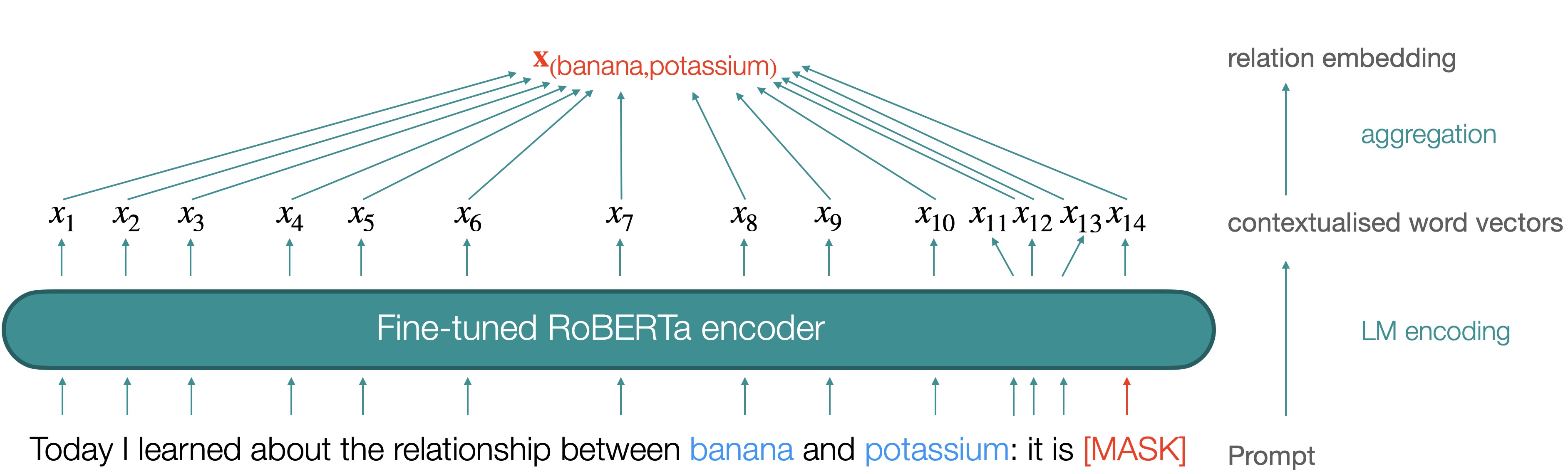
Figure 1: Schematic overview of the RelBERT model. A word pair is presented to an LM encoder using a prompt. A relation vector, capturing how the two input words are related, is then obtained by aggregating the contextualised embeddings from the output layer.

§ 3.1 Overall Strategy

To obtain the relation embedding of a word pair $(h,t)$, we need to construct a suitable input for the language model. While it is possible to simply use the pair $(h,t)$ as input, similar to what is done by COMET [89], better results can be achieved by converting the word pair into a more or less naturally sounding sentence. This is true, in particular, because the amount of high-quality data that is available for training RelBERT is relatively limited, as we will see in § 3.3. We thus need to manually create a template with placeholders for the two target words, which somehow expresses that we are interested in modelling the relationship between the two words. Such a strategy has already been proven effective for factual knowledge probing [18] and text classification [90, 91, 92], among many others. Since we will rely on fine-tuning the LM, the exact formulation of the prompt matters less than in zero-shot settings. However, we found that performance suffers when the prompt is too short, in accordance with [61] and [19], or when the prompt is nonsensical (i.e. when it does not express the idea of modelling a relationship). With this in mind, we will use the following five templates for our main experiments:

1. Today, I finally discovered the relation between [h] and [t] : [h] is the <mask> of [t]

2. Today, I finally discovered the relation between [h] and [t] : [t] is [h]’s <mask>

3. Today, I finally discovered the relation between [h] and [t] : <mask>

4. I wasn’t aware of this relationship, but I just read in the encyclopedia that [h] is the <mask> of [t]

5. I wasn’t aware of this relationship, but I just read in the encyclopedia that [t] is [h]’s <mask>

where <mask> is the LM’s mask token, and [h] and [t] are slots that are filled with the head word $h$ and tail word $t$ from the given word pair. As a final step, we construct the relation embedding $\mathbf{x}_{(h,t)}$ from the contextualised representation of the prompt in the LM’s output layer. In particular, we have experimented with the following three strategies:

• We take the contextualised representation of the <mask> token as the relation embedding (average).

• We average the contextualised embeddings across all tokens from the prompt (mask).

• We average the contextualised embeddings across all tokens from the prompt except for the <mask> token (average w.o. mask).

In the following we explain the training objectives and how the model is trained.

§ 3.2 Training Objective

The LM encoder used in RelBERT is initialised from a pre-trained RoBERTa model, which was shown to be more effective than BERT in our previous work [46]. It is then fine-tuned using a contrastive loss, based on the idea that word pairs which belong to the same relation should have a relation embedding that is similar, whereas word pairs belonging to different relations should have embeddings that are further apart. To this end, we assume access to a set of positive training examples $\mathcal{P}_{r}$ and a set of negative examples $\mathcal{N}_{r}$, for a number of relations $r\in\mathcal{R}$. In particular, $\mathcal{P}_{r}$ contains word pairs $(h,t)$ which belong to relation $r$, whereas $\mathcal{N}_{r}$ contains examples of word pairs which do not. We consider three different loss functions to implement the proposed idea.

Triplet Loss

The triplet loss [94] relies on training data in the form of triples $(a,p,n)$, where $a$ is called the anchor, $p$ is a positive example, and $n$ is a negative example. The aim of this loss is to ensure that the distance between $a$ and $p$ is smaller, by some margin, than the distance between $a$ and $n$. In our case, the elements $a$, $p$ and $n$ correspond to word pairs, where $a,p\in\mathcal{P}_{r}$ and $n\in\mathcal{N}_{r}$ for some relation $r$. Let us write $\bm{x}_{a}$ for the relation embedding of a word pair $a$. We then have the following loss:

$$L_{{\rm tri}}=\sum_{r\in\mathcal{R}}\sum_{(a,p,n)\in\mathcal{P}_{r}\times\mathcal{P}_{r}\times\mathcal{N}_{r}}\max\big{(}0,\|\bm{x}_{a}-\bm{x}_{p}\|-\|\bm{x}_{a}-\bm{x}_{n}\|+\Delta\big{)}$$ (1)

where $\Delta>0$ is the margin and $\|\cdot\|$ is the $l^{2}$ norm.

InfoNCE

Information noise constrastive estimation (InfoNCE) [95] addresses two potential limitations of the triplet loss. First, while the triplet loss only considers one negative example at a time, InfoNCE can efficiently contrast each positive example to a whole batch of negative examples. Second, while the triplet loss uses the $l^{2}$ norm, InfoNCE relies on the cosine similarity, which tends to be better suited for comparing embeddings. The InfoNCE loss can be defined as follows:

$$L_{{\rm nce}}=\sum_{r\in\mathcal{R}}\sum_{(a,p)\in\mathcal{P}_{r}\times\mathcal{P}_{r}}\left(-\log\frac{\exp{\left(\frac{{\rm cos}(\bm{x}_{a},\bm{x}_{p})}{\tau}\right)}}{\exp{\left(\frac{{\rm cos}(\bm{x}_{a},\bm{x}_{p})}{\tau}\right)}+\sum_{n\in\mathcal{N}_{r}}\exp{\left(\frac{{\rm cos}(\bm{x}_{a},\bm{x}_{n})}{\tau}\right)}}\right)$$ (2)

where $\tau$ is a temperature parameter to control the scale of the exponential and cos is the cosine similarity.

InfoLOOB

Info-leave-one-out-bound (InfoLOOB) [96] is a variant of InfoNCE, in which the positive example is omitted from the denominator. This is aimed at preventing the saturation of the loss value, which can occur with InfoNCE due to dominant positives. Applied to our setting, the loss is as follows:

$$L_{{\rm loob}}=\sum_{r\in\mathcal{R}}\sum_{(a,p)\in\mathcal{P}_{r}\times\mathcal{P}_{r}}\left(-\log\frac{\exp{\left(\frac{{\rm cos}(\bm{x}_{a},\bm{x}_{p})}{\tau}\right)}}{\sum_{n\in\mathcal{N}_{r}}\exp{\left(\frac{{\rm cos}(\bm{x}_{a},\bm{x}_{n})}{\tau}\right)}}\right)$$ (3)

Dataset	RelSim	ConceptNet	NELL	T-REX
#relations (train/val/test)	89/89/-	28/18/16	31/4/6	721/602/24
Average #positive examples per relation	14.7/3.7/-	20,824/66/74	177/219/225	1,767/529/4
Relation Hierarchy	True	False	False	False
Domain	Concepts	Concepts	Named entities	Named entities

Table 2: Statistics of the training sets that are considered for RelBERT, including the number of relations, the average number of triples per relation in the training / validation / test sets, and the number of unique positive triples; we also specify whether the relations are organised in a hierarchy, the domain from which the entities are coming.

§ 3.3 Training Data

As described in § 3.2, to train RelBERT we need positive and negative examples of word pairs belonging to particular relations. In this section, we describe the four datasets that we considered for training RelBERT. The main properties of these datasets are summarised in Table 2. We now present each dataset in more detail. For each dataset, we have a training and validation spit, which are used for training RelBERT and for selecting the hyperparameters. In addition, for most of the datasets, we also select a test set, which will be used for evaluating the model (see § 4.1).

Relation	Examples
Case Relation	[designer, fashions], [preacher, parishioner], [hunter, rifle]
Meronym (Part-Whole)	[building, wall], [team, player], [movie, scene]
Antonym (Contrast)	[smooth, rough], [difficult, easy], [birth, death]
Space-Time	[refrigerator, food], [factory, product], [pool, swimming]
Representation	[diploma, education], [groan, pain], [king, crown]
Hypernym (Class Inclusion)	[furniture, chair], [furniture, chair], [flower, daisy]
Synonym (Similar)	[couch, sofa], [sadness, melancholia], [confident, arrogance]
Attribute	[steel, strong], [glass, shattered], [miser, greed]
Non Attribute	[empty, full], [incomprehensible, understood], [destitution, abundance]
Cause-Purpose	[tragedy, tears], [fright, scream], [battery, laptop]

Table 3: Examples of word pairs from each parent relation category in the RelSim dataset.

RelSim

The Relational Similarity Dataset (RelSim) was introduced for SemEval 2012 Task 2 [25]. It contains crowdsourced judgements about 79 fine-grained semantic relations, which are grouped into 10 parent categories. Table 3 shows word pairs randomly sampled from the highest ranked word pairs in each parent category of RelSim. For each semantic relation, a list of word pairs is provided in RelSim, with each word pair being assigned a prototypicality score. To convert this dataset into the format that we need for training RelBERT, we consider the 79 fine-grained relations and the 10 parent relations separately. For the fine-grained relations, we choose the 10 most prototypical word pairs, i.e. the word pairs with the highest scores, as positive examples, while the 10 lowest ranked word pairs are used as negative examples. For the parent relations, the set of positive examples contains the positive word pairs of each of the fine-grained relations that belong to the parent relation. The negative examples for the parent relations are taken to be the positive examples of the other relations. This is because the parent relations are mutually exclusive, whereas the semantic distinction between the fine-grained relations is often very subtle. From the resulting dataset, we randomly choose 80% of the word pairs for training, and we keep the remaining 20% as a validation set.

ConceptNet

ConceptNet [97] is a commonsense knowledge graph. It encodes semantic relations between concepts, which can be single nouns or short phrases. The knowledge graph refers to a total of 34 different relations. Since the original ConceptNet contains more than two millions of triples, we employ the version released by [98], where the triples are filtered by their confidence score. We use the test set consisting of the 1200 most confident tuples as an evaluation dataset, the dev1 and dev2 sets consisting of the next 1200 most confident tuples as our validation set, and the training set consisting of 600k tuples as our training set. We have disregarded any triples with negated relations such as NotCapableOf or NotDesires, because they essentially indicate the lack of a relationship. The positive examples for a given relation are simply the word pairs which are asserted to have this relation in the knowledge graph. The negative examples for a given relation are taken to be the positive examples for the other relations, i.e. $\mathcal{N}_{r}=\{(a,b)\in\mathcal{P}_{\hat{r}}|\hat{r}\in\mathcal{R}\setminus\{r\}\}$.

NELL-One

NELL [99] is a system to collect structured knowledge from web. The authors of [100] compiled and cleaned up the latest dump file of NELL at the time of publication to create a knowledge graph, called NELL-One for one-shot relational learning. We employ NELL-One with its original split from [100], which avoids any overlap between the relation types appearing in the test set, on the one hand, and the relation types appearing in the training and validation sets, on the other hand. Similar as for ConceptNet, the positive examples for a given relation are the word pairs that are asserted to belong to that relation in the training set, whereas the negative examples for a relation are the positive examples of the other relations in the training set.

T-REX

T-REX [101] is a knowledge base that was constructed by aligning Wikipedia and Wikidata. It contains a total of 20 million triples, all of which are aligned with sentences from introductory sections of Wikipedia articles. We first remove triples if either their head or tail is not a named entity, which reduces the number of triples from 20,877,472 to 12,561,573, and the number of relations from 1,616 to 1,470. Then, we remove relations with fewer than three triples, as we need at least three triples for each relation type to enable fine-tuning § 5.1, which reduces the number of triples to 12,561,250, and the number of relations to 1,237. One problem with this dataset is that it contains a number of distinct relations which intuitively have the same meaning. For example, the relations band and music by both represent “A song played by a musician”. Therefore, we manually mapped such relations onto the same type. Note that this is useful because the strategy for selecting negative examples when training RelBERT implicitly assumes that relations are disjoint. For the same reason, we manually removed relations that subsume more specific relations. For example, the relationship is a refers to “hypernym of”, but T-REX also covers more specific forms of hypernymy such as fruit of, religion, and genre. Another example is is in, which models the relation “located in”, but T-REX also contains finer-grained variants of this relation, such as town, state, home field, and railway line. We thus remove triples involving relations such as is a and is in. This filtering resulted in a reduction to 12,410,726 triples with 839 relation types. We use this dataset, rather than Wikidata itself, because the fact that a triple is asserted in the introductory section of a Wikipedia article suggests that it expresses salient knowledge. This is important because our aim in fine-tuning RelBERT is to distill relational knowledge from the pre-trained LM itself, rather than to learn the knowledge from the training set. We thus ideally want to limit the training data to word pairs whose relationship is captured by the pre-trained LM. The number of times an entity appears in this dataset can be used as an estimate of the salience of that entity. With this in mind, we removed all triples involving entities that appear less than five times in the dataset, which further reduces the number of triples to 1,616,065. To create a test set, we randomly chose 34 relation types and we manually selected around 100 verified triples from those relation types. The training and validation set is created by splitting the remaining relations 80:20 into a training and validation set.

§ 4 Evaluation Tasks

We evaluate RelBERT on two relation-centric tasks: analogy questions (unsupervised), and lexical relation classification (supervised). In this section, we describe these tasks and introduce the benchmarks included in our evaluation.

§ 4.1 Analogy Questions

Dataset	Avg. #Answer Candidates	#Questions
SAT	5/5	- / 374
U2	4/4	24 / 228
U4	4/4	48 / 432
Google	4/4	50 / 500
BATS	4/4	199 / 1,799
SCAN	72/74	178 / 1,616
NELL-One	5/7	400 / 600
T-REX	74/48	496 / 183
ConceptNet	19/17	1,112 / 1,192

Table 4: Main statistics of the analogy question datasets, showing the average number of answer candidates, and the total number of questions (validation / test).

Dataset	Domain	Example
SAT	College Admission Test	[beauty, aesthete, pleasure, hedonist]
U2	Grade4	[rock, hard, water, wet]
	Grade5	[hurricane, storm, table, furniture]
	Grade6	[microwave, heat, refrigerator, cool]
	Grade7	[clumsy, grace, doubtful, faith]
	Grade8	[hidden, visible, flimsy, sturdy]
	Grade9	[panacea, cure, contagion, infect]
	Grade10	[grain, silo, water, reservoir]
	Grade11	[thwart, frustrate, laud, praise]
	Grade12	[lie, prevaricate, waver, falter]
U4	Low Intermediate	[accident, unintended, villain, evil]
	Low Advanced	[galleon, sail, quarantine, isolate]
	High Beginning	[salesman, sell, mechanic, repair]
	High Intermediate	[classroom, desk, church, pew]
	High Advanced	[erudite, uneducated, fervid, dispassionate]
BATS	Inflectional Morphology	[neat, neater, tasty, tastier]
	Derivational Morphology	[available, unavailable, interrupted, uninterrupted]
	Encyclopedic Semantics	[stockholm, sweden, belgrade, serbia]
	Lexicographic Semantics	[elephant, herd, flower, bouquet]
Google	Encyclopedic Semantics	[Canada, dollar, Croatia, kuna]
	Morphological	[happy, happily, immediate, immediately]
SCAN	Metaphor	[grounds for a building, solid, reasons for a theory, rational]
	Science	[conformance, breeding, adaptation, mating]
NELL	Named Entities	[Miami Dolphins, Cam Cameron, Georgia Tech, Paul Johnson]
T-REX	Named Entities	[Washington, Federalist Party, Nelson Mandela, ANC]
ConceptNet	Concepts	[bottle, plastic, book, paper]

Table 5: An example from each domain of the analogy question benchmarks.

Analogy questions are multiple-choice questions, where a given word pair is provided, referred to as the query pair, along with a set of candidate answers. Then, the task consists of predicting which is the word pair that is most analogous to the query pair among the given candidate answers. In other words, the task is to find the word pair whose relationship best resembles the relationship between the words in the query [11].

To solve this task using RelBERT, we simply predict the candidate answer whose relation embedding is most similar to the embedding of the query pair, in terms of cosine similarity. For our evaluation, first, we consider the following six analogy question datasets:

SAT

The SAT exam is a US college admission test. Turney [11] collected a benchmark of 374 word analogy problems, consisting primarily of problems from these SAT tests. Each instance has five candidates. The instances are aimed at college applicants, and are thus designed to be challenging for humans.

U2

Following [102], who used word analogy problems from an educational website, we compiled analogy questions from the same resource. They used in particular UNIT 2 of the analogy problems from the website, which have the same form as those from the SAT benchmark, but rather than college applicants, they are aimed at children in grades 4 to 12 from the US school system (i.e. from age 9 onwards). We split the dataset into 24 questions for validation and 228 questions for testing. Each question has 4 answer candidates.

U4

We have collected another benchmark from the UNIT 4 problems on the same website that was used for the U2 dataset. These UNIT 4 problems are organised in 5 difficulty levels: high-beginning, low-intermediate, high-intermediate, low-advanced and high-advanced. The low-advanced level is stated to be at the level of the SAT tests, whereas the high-advanced level is stated to be at the level of the GRE test (which is used for admission into graduate schools). The resulting U4 dataset has 48 questions for validation and 432 questions for testing. Each question has 4 answer candidates.

Google

The Google analogy dataset [103] has been one of the most commonly used benchmarks for evaluating word embeddings. This dataset contains a mix of semantic and morphological relations such as capital-of and singular-plural, respectively. The dataset was tailored to the evaluation of word embeddings in a predictive setting. We constructed word analogy problems from the Google dataset by choosing for each correct analogy pair a number of negative examples. To obtain sufficiently challenging negative examples, for each query pair (e.g. Paris-France) we extracted three negative instances:

1. two random words from the head of the input relation type (e.g. Rome-Oslo);

2. two random words from the tail of the input relation type (e.g. Germany-Canada);

3. a random word pair from a relation type of the same high-level category (i.e. semantic or morphological) as the input relation type (e.g. Argentina-peso).

The resulting dataset contains 50 validation and 500 test questions, each with 4 answer candidates.

BATS

The coverage of the Google dataset is known to be limiting, and BATS [6] was developed in an attempt to address its main shortcomings. BATS includes a larger number of concepts and relations, which are split into four categories: lexicographic, encyclopedic, and derivational and inflectional morphology. We follow the same procedure as for the Google dataset to convert BATS into the analogy question format. The resulting dataset contains 199 validation and 1,799 test questions, each with 4 answer candidates.

SCAN

The relation mapping problem [104] is to find a bijective mapping between a set of relations from some source domain and a corresponding set of relations from a given target domain. SCAN [105] is an extension of the problems that were collected in [104]. Where [104] contains 10 scientific and 10 metaphorical domains, SCAN extends them by another 443 metaphorical domains and 2 scientific domains. A single SCAN instance contains a list of the source and the target words ($\bm{a}=[a_{1},\dots,a_{m}]$ and $\bm{b}=[b_{1},\dots,b_{m}]$). We convert such an instance into an analogy question, where the query is $[a_{i},a_{j}]$ and the ground truth is $[b_{i},b_{j}]$ and the negative candidates are $[b_{\hat{i}},b_{\hat{j}}]$ for $\{(\hat{i},\hat{j})\in\{1,\dots,m\}\times\{1,\dots,m\}|(\hat{i},\hat{j})\neq(i,j)\}$. This results in 178 and 1,616 questions for the validation and test sets, respectively. The number of answer candidates per question is 74 on average, which makes this benchmark particularly challenging.

In addition, we also converted the validation and test splits of T-REX, NELL and ConceptNet, which were introduced in § 3.3, into the format of analogy questions. Note that the validation split is used in our ablation study to compare RelBERT training sets, but not used in the main experiment, where we solve analogy questions in the zero-shot setting. Thus, we do not consider approaches that require validation as well as training data, such as [12]. These analogy questions were constructed by taking two word pairs from the same relation type, one of which is used as the query while the other is used as the correct answer. To create negatives for each positive pair, we take $N$ pairs from each of the other relations. We also add the reversed answer pair to the negative (i.e. for the positive pair $(h,t)$ we would add $(t,h)$ as a negative), so the number of the negative pairs is $|\mathcal{R}|\times N+1$ in each split. To create benchmarks with different characteristics, we used $N=2$ for T-REX and $N=1$ for Nell and ConceptNet.

Table 4 summarises the main features of the analogy question datasets, and Table 5 shows an example from each category and dataset.

§ 4.2 Lexical Relation Classification

	BLESS	CogALex	EVALution	K&H+N	ROOT09
Antonym	-	241 / 360	1095 / 90 / 415	-	-
Attribute	1892 / 143 / 696	-	903 / 72 / 322	-	-
Co-hyponym	2529 / 154 / 882	-	-	18134 / 1313 / 6349	2222 / 162 / 816
Event	2657 / 212 / 955	-	-	-	-
Hypernym	924 / 63 / 350	255 / 382	1327 / 94 / 459	3048 / 202 / 1042	2232 / 149 / 809
Meronym	2051 / 146 / 746	163 / 224	218 / 13 / 86	755 / 48 / 240	-
Possession	-	-	377 / 25 / 142	-	-
Random	8529 / 609 / 3008	2228 / 3059	-	18319 / 1313 / 6746	4479 / 327 / 1566
Synonym	-	167 / 235	759 / 50 / 277	-	-

Table 6: Number of instances for each relation type across training / validation / test sets of all lexical relation classification datasets.

We consider the supervised task of relation classification. This task amounts to classifying word pairs into a predefined set of possible relation types. To solve this task, we train a multi-layer perceptron (MLP) with one hidden layer, which takes the RelBERT relation embedding of the word pair as input. The RelBERT encoder itself is frozen, since our focus is on evaluating the quality of the RelBERT relation embeddings. We consider the following widely-used multi-class relation classification benchmarks: K&H+N [106], BLESS [107], ROOT09 [108], EVALution [109], and CogALex-V Subtask 2 [110]. Table 6 shows the size of the training, validation and test splits for each of these datasets, as well as the kinds of relations they cover. The hyperparameters of the MLP classifier are tuned on the validation split of each dataset. In particular, we tune the learning rate from $[0.001,0.0001,0.00001]$ and the hidden layer size from $[100,150,200]$. CogALex-V has no validation split, so for this dataset we employ the default configuration of Scikit-Learn [111], which uses a 100-dimensional hidden layer and is optimized using Adam with a learning rate of 0.001.

§ 5 Experimental Setting

In this section, we explain the RelBERT training details (§ 5.1) and we introduce the baselines for analogy questions (§ 5.2) and lexical relation classification (§ 5.3). Throughout this paper, we rely on the weights that were shared by HuggingFace [112] for all pre-trained LMs. A complete list of the models we used can be found in A.

§ 5.1 RelBERT Training

In our experiments, we consider a number of variants of RelBERT, which differ in terms of the pre-trained LM that was used for initialising the model, the loss function § 3.2, and the training data § 3.3. In each case, RelBERT is trained for 10 epochs. Moreover, we train one RelBERT model for each of the five prompt templates § 3.1. The final model is obtained by selecting the epoch and prompt template that achieved the best performance on the validation split, in terms of accuracy. The default configuration for RelBERT is to fine-tune a RoBERTa_BASE or RoBERTa_LARGE model using InfoNCE on the RelSim dataset. We will refer to the resulting models as RelBERT_BASE and RelBERT_LARGE respectively. The other hyper-parameters are fixed as follows. When using the triplet loss, we set the margin $\Delta$ to 1, the learning rate to 0.00002 and the batch size to 32. When using InfoNCE or InfoLoob, we set the temperature $\tau$ to 0.5, the learning rate to 0.000005 and the batch size to 400. In all cases, we fix the random seed as 0 and we use ADAM [113] as the optimiser. To select the aggregation strategy, as a preliminary experiment, we fine-tuned RelBERT_BASE with each of the three strategies suggested in § 3.2. As we found that average w.o. mask achieved the best accuracy on the validation set of RelSim, we used this as the default aggregation strategy.

§ 5.2 Baselines for Analogy Questions

We now introduce the baselines we considered for solving analogy questions.

Latent Relation Analysis

Latent Relation Analysis (LRA) [1] takes inspiration from the seminal Latent Semantic Analysis (LSA) model for learning document embeddings [114]. The key idea behind LSA was to apply Singular Value Decomposition (SVD) on a document-term co-occurrence matrix to obtain low-dimensional vector representations of documents. LRA similarly uses SVD to learn relation vectors. In particular, the method also constructs a co-occurrence matrix, where the rows now correspond to word pairs and the columns correspond to lexical patterns. Each matrix entry captures how often the corresponding word pair appears together with the corresponding lexical pattern in a given corpus. To improve the quality of the representations, a PMI-based weighting scheme is used, and the method also counts occurrences of synonyms of the words in a given pair. To solve an analogy question, we can compute the LRA embeddings of the query pair and the candidate pairs, and then select the answer whose embedding is closest to the embedding of the query pair, in terms of cosine similarity. For LRA, we only report the published results from [1] for the SAT dataset.

Word Embedding

Since the introduction of the Word2Vec models [3], word analogies have been a popular benchmark for evaluating different word embedding models. This stems from the observation that in many word embedding models, the relation between two words $A$ and $B$ is to some extent captured by the vector difference of their embeddings. Letting $\mathsf{wv}(A)$ be the word embedding of a word $A$, we can thus learn relation embeddings of the form $\mathbf{x}_{(A,B)}=\mathsf{wv}(B)-\mathsf{wv}(A)$. Using these embeddings, we can solve word analogy questions by again selecting the answer candidate whose embedding is most similar to that of the query pair, in terms of cosine similarity. Since some of the analogy questions include rare words, common word embedding models such as word2vec [3] and GloVe [4] suffer from out-of-vocabulary issues. We therefore used fastText [5] trained on Common Crawl with subword information, which can handle out-of-vocabulary words by splitting them into smaller chunks of characters.

Language Models

To solve analogy questions using a pre-trained language model, we proceed as follows. Let $(A,B)$ be the query pair. For each answer candidate $(C,D)$ we construct the sentence “A is to B what C is to D”, following [16]. We then compute the perplexity of each of these sentences, and predict the candidate that gives rise to the lower perplexity. The exact computation depends on the type of language model that is considered. For CLMs [115, 116, 16], such as those in the GPT family, the perplexity of a sentence ${\bm{s}}$ can be computed as follows:

$$f({\bm{s}})=\exp\left(-\frac{1}{t}\sum_{j=1}^{t}\log{P_{\text{clm}}(s_{j}|{\bm{s}}_{j-1})}\right)$$ (4)

where ${\bm{s}}$ is tokenized as $[s_{1}...s_{t}]$ and $P_{\text{clm}}(s|{\bm{s}})$ is the likelihood from an CLM’s next token prediction. For masked language models (MLMs), such as those in the BERT family [15, 24], we instead use pseudo-perplexity [117], which is defined as in (4) but with $P_{\text{mask}}(s_{j}|{\bm{s}}_{\backslash j})$ instead of $P_{\text{clm}}(s_{j}|{\bm{s}}_{j-1})$, where ${\bm{s}}_{\backslash j}=[s_{1}\dots s_{j_{1}}\text{\textlangle mask\textrangle}s_{j+1}\dots s_{t}]$ and $P_{\text{mask}}(s_{j}|{\bm{s}}_{\backslash j})$ is the pseudo-likelihood [118] that the masked token is $s_{j}$. Finally, for encoder-decoder LMs (ED LMs) [17, 119], we split the template in two parts: the phrase “A is to B” is fed into the encoder, and then we use the decoder to compute the perplexity of the phrase “C is to D”, using the probability $P_{\text{clm}}$ of the decoder, conditioned by the encoder. We compare GPT-2 [116], GPT-J [120], OPT [26], OPT-IML [27] as CLMs, BERT [15] and RoBERTa [24] as MLMs, and T5 [17], Flan-T5 [28], Flan-UL2 [121] as ED LMs.

OpenAI Models

OpenAI released a commercial API to provide access to their private in-house models such as GPT-3, GPT-4, and ChatGPT (GPT-3.5-turbo). We have used this API to obtain results for those models. For GPT-3, we use the May 2023 endpoint of davinci, the largest GPT-3 model, and follow the same approach as for the public LMs, as explained above (i.e. choose the candidate with the lowest perplexity). We also include the zero-shot results of GPT-3 that were reported in the original GPT-3 paper [16], which we refer as GPT-3_original. Note that the models that can be accessed via the OpenAI API are subject to be changed every six months, which unfortunately limits the reproducibility of the reported results. For the conversational LMs, i.e. ChatGPT and GPT-4, the API does not allow us to compute perplexity scores. We therefore do not include them in our main experiments, but an analysis of these models will be provided in § 7.2.1.

§ 5.3 Baselines for Lexical Relation Classification

LexNet [122] and SphereRE [123] are the current state-of-the-art (SotA) classifiers on the considered lexical relation classification datasets. Both methods rely on static word embeddings [3, 124]. LexNet trains an LSTM [125] on the word pair by considering it as a sequence of two words, where each word is mapped to its feature map consisting of a number of lexical features such as part-of-speech and the word embedding. SphereRE employs hyperspherical learning [126] on top of the word embeddings, which is to learn a feature map from word embeddings of the word pairs to their relation embeddings, which are distributed over the hyperspherical space. In addition to those SotA methods, we use a simple baseline based on word embeddings. Specifically, we train an MLP with a hidden layer in the same way as explained in § 4.2. As possible input representations for this classifier, we consider the concatenation of the word embeddings (cat) and the vector difference of the word embeddings (diff), possibly augmented with the component-wise product of the word embeddings (cat+dot and diff+dot), which has been shown to provide improvements in lexical relation classification tasks [127]. We experiment with word embeddings from GloVE [4] and fastText. Finally, we include the results of pair2vec [54], which is a relation embedding model that was trained by aligning word pair embeddings with LSTM-based encodings of sentences where the corresponding word pairs co-occur.

	Model	SAT	U2	U4	BATS	Google	SCAN	NELL	T-REX	CN	Average
Random		20.0	23.6	24.2	25.0	25.0	2.5	14.3	2.1	5.9	15.8
LRA		56.4	-	-	-	-	-	-	-	-	-
fastText		47.1	38.2	38.4	70.7	94.6	21.7	59.8	23.0	15.2	45.1
MLM	BERTBASE	34.5	35.1	35.2	48.4	67.6	14.5	25.2	9.8	9.4	31.1
	BERTLARGE	32.9	36.0	36.6	59.4	79.8	14.1	32.0	14.2	14.0	35.4
	RoBERTaBASE	36.4	42.1	43.3	61.8	81.0	10.6	29.0	14.8	16.6	37.3
	RoBERTaLARGE	40.6	50.4	49.8	69.9	88.8	12.1	38.2	36.1	16.7	44.7
Causal LM	GPT-2SMALL	32.1	38.2	36.8	43.6	56.8	5.1	28.5	7.1	8.1	28.5
	GPT-2BASE	34.8	42.5	40.5	58.3	75.8	7.0	43.8	6.6	11.6	35.7
	GPT-2LARGE	36.1	42.1	42.6	60.1	75.4	8.8	39.0	12.6	12.8	36.6
	GPT-2XL	36.9	43.0	44.0	62.0	80.4	8.2	40.2	11.5	12.6	37.6
	GPT-J125M	34.0	36.8	35.6	46.6	52.8	5.6	31.8	10.9	8.4	29.2
	GPT-J1.3B	36.6	42.1	42.1	63.1	77.0	8.8	47.3	13.1	11.7	38.0
	GPT-J2.7B	38.5	44.7	43.5	63.8	83.0	8.8	40.0	16.9	14.1	39.3
	GPT-J6B	45.5	48.7	47.0	67.9	87.4	9.5	43.8	20.2	14.0	42.7
	GPT-J20B	42.8	47.8	53.7	71.3	86.4	10.0	37.2	31.7	15.7	44.1
	GPT-3original*	53.7	-	-	-	-	-	-	-	-	-
	GPT-3davinci*	51.8	53.5	53.2	70.8	86.0	0.84	37.8	20.7	14.2	43.9
	OPT125M	33.7	37.3	35.4	46.1	60.0	7.1	39.7	10.4	10.8	31.2
	OPT350M	34.0	36.8	39.1	54.8	74.2	8.2	44.7	10.9	10.6	34.8
	OPT1.3B	38.5	40.4	43.5	62.8	83.4	8.8	46.3	11.5	14.8	38.9
	OPT30B	47.1	52.2	51.9	71.5	88.2	10.5	45.2	20.8	19.1	45.2
	OPT-IML1.3B	41.4	42.5	44.9	63.1	82.4	8.1	42.0	7.7	14.8	38.5
	OPT-IML30B	48.9	50.2	49.0	70.8	88.3	10.8	44.4	23.2	17.5	44.8
	OPT-IMLM-1.3B	40.6	40.8	44.0	64.1	85.4	9.0	45.7	8.2	15.9	39.3
	OPT-IMLM-30B	48.9	50.2	49.0	70.8	88.3	10.8	44.4	23.2	17.5	44.8
Encoder Decoder LM	T5SMALL	28.9	32.9	30.6	41.0	55.4	17.0	38.0	15.8	5.8	29.5
	T5BASE	26.7	34.6	39.8	43.0	41.4	9.9	27.8	6.0	7.7	26.3
	T5LARGE	30.2	35.5	40.0	48.9	51.4	13.7	25.2	11.5	9.1	29.5
	T53B	34.8	35.1	35.4	41.6	45.8	10.2	25.3	20.8	9.0	28.7
	T511B	35.6	43.0	47.5	59.9	74.6	17.9	40.8	27.3	13.8	40.0
	Flan-T5SMALL	26.7	36.4	41.7	42.7	49.0	11.6	35.5	16.9	8.3	29.9
	Flan-T5BASE	31.8	38.6	42.1	51.4	63.6	13.7	38.8	20.8	9.6	34.5
	Flan-T5LARGE	36.1	40.8	43.5	52.6	63.8	13.4	38.0	20.8	11.3	35.6
	Flan-T5XL	42.0	49.6	50.7	66.8	86.8	17.6	46.0	30.6	17.0	45.2
	Flan-T5XXL	52.4	55.7	55.6	74.7	91.2	16.3	43.8	26.8	17.9	48.3
	Flan-UL2	50.0	53.1	57.2	74.9	91.8	13.4	53.8	36.1	16.8	49.7
RelBERTBASE		59.9	59.6	57.4	70.3	89.2	25.9	62.0	66.7	39.8	59.0
RelBERTLARGE		73.3	67.5	63.0	80.9	95.2	27.2	65.8	64.5	47.5	65.0

Table 7: The accuracy on each analogy question dataset and the averaged accuracy across datasets, where the best model in each dataset shown in bold. Result in italics were taken from the original paper, and the model with * are private models.

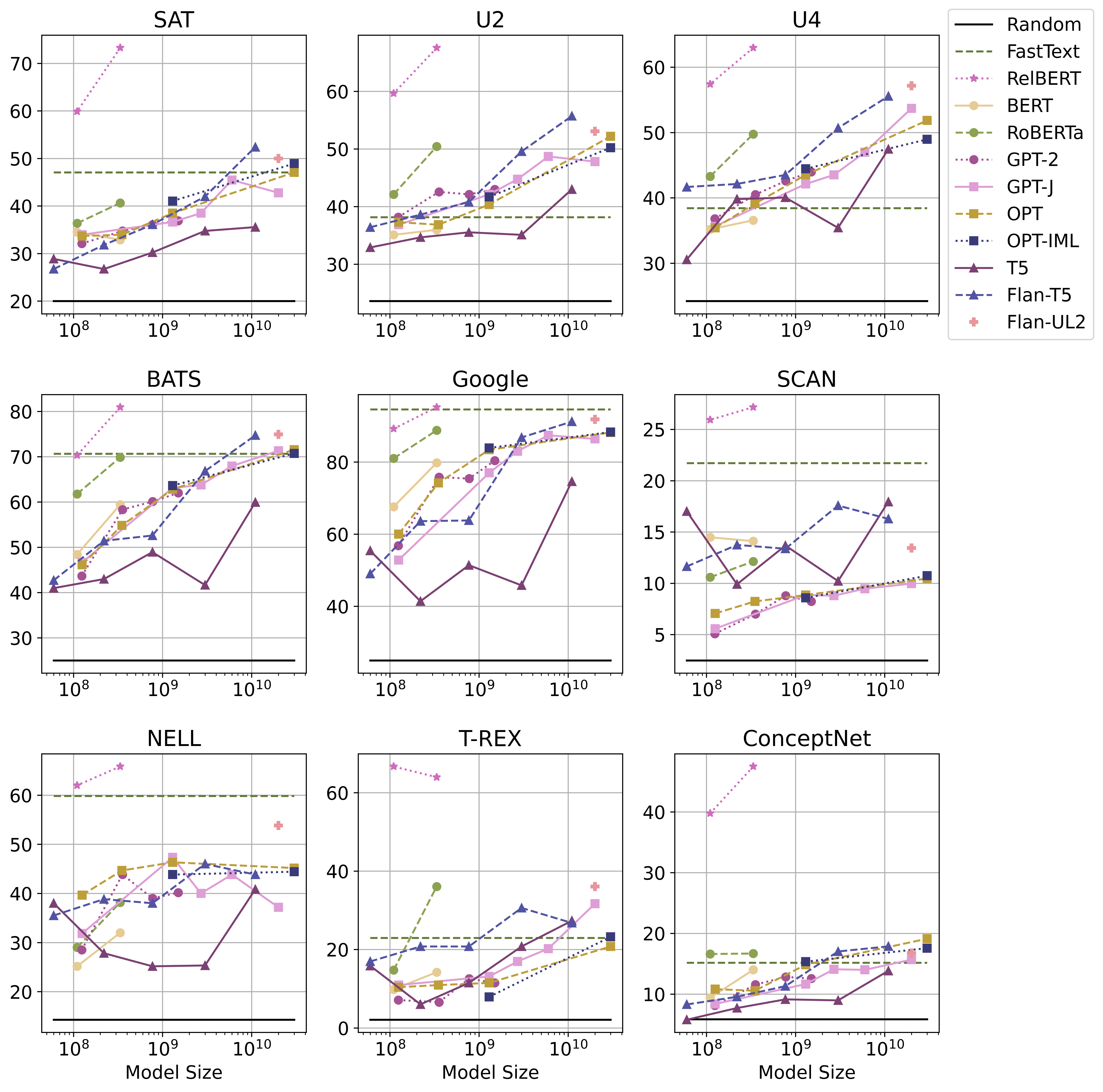
Figure 2: The accuracy on each analogy question dataset in function of the number of parameters in each LM.

Model		BLESS	CogALexV	EVALution	K&H+N	ROOT09
pair2vec		81.7	76.9	50.5	96.9	82.9
GloVe	cat	93.3	73.5	58.3	94.9	86.5
	cat+dot	93.7	79.2	57.3	95.1	89.0
	cat+dot+pair2vec	92.6	81.1	59.6	95.7	89.4
	diff	91.5	70.8	56.9	94.4	86.3
	diff+dot	92.9	78.5	57.9	94.8	88.9
	diff+dot+pair2vec	92.2	80.2	57.4	95.5	89.4
fastText	cat	92.9	72.4	57.9	93.8	85.5
	cat+dot	93.2	77.4	57.8	94.0	88.5
	cat+dot+pair2vec	91.5	79.3	58.2	94.3	87.8
	diff	91.2	70.2	55.5	93.3	86.0
	diff+dot	92.9	77.8	57.4	93.6	88.9
	diff+dot+pair2vec	90.8	79.0	57.8	94.2	88.1
SotA	LexNET	89.3	-	60.0	98.5	81.3
	SphereRE	93.8	-	62.0	99.0	86.1
RelBERTBASE		90.0	83.7	64.2	94.0	88.2
RelBERTLARGE		92.0	85.0	68.4	95.6	90.4

Table 8: Micro F1 score (%) for lexical relation classification.

§ 6 Experimental Results

We report the experimental results for the analogy questions benchmarks in § 6.1 and for lexical relation classification in § 6.2.

§ 6.1 Results on Analogy Questions

Table 7 shows the results for each analogy question benchmark in terms of accuracy. We can see that RelBERT substantially outperforms the baselines in all cases, where RelBERT_BASE is the best for T-REX, and RelBERT_LARGE is the best for the remaining datasets. Remarkably, in the case of SAT, none of the pre-trained LMs is able to outperform LRA, a statistical baseline which is almost 20 years old. Moreover, on the Google, SCAN and NELL datasets the LM baselines are outperformed by fastText, a static word embedding model. This clearly shows that LMs struggle with identifying analogies in the zero-shot setting. SCAN and ConceptNet overall emerge as the most challenging benchmarks, which can be largely explained by the large number of answer candidates. Even with the best model, RelBERT_LARGE, the accuracy is only 27.2% on SCAN and 47.5% on ConceptNet. For T-REX, which also involves a large number answer candidates, we can see that the LM baselines are clearly outperformed by RelBERT. Comparing the LM baselines, we find that ED LMs such as Flan-T5_XXL and Flan-UL2 achieve the best overall results, although CLMs such as GPT-J and OPT_20B are also competitive among the larger models.

For the LM baselines, unsurprisingly there is a strong correlation between model size and performance. To see this impact more closely, Figure 2 plots the accuracy of each LM in function of model size. We can see that the RelBERT models achieve the best result despite being two orders of magnitude smaller than Flan-T5_XXL and Flan-UL2. Interestingly, RoBERTa usually outperforms the other LM baselines of comparable size, except on NELL and SCAN. This suggests that the strong performance of RelBERT is at least in part due to the use of RoBERTa as the underlying model. Our analysis in § 7.3.4 will provide further support for this hypothesis. The CLMs (GPT-2, GPT-J, OPT, and OPT-IML) behave rather similarly. They improve as the model size increases, but they are generally worse than the ED LMs and MLMs. Finally, the graphs in Figure 2 make it particularly clear how much the LMs are struggling to compete with fastText in some of the datasets. For example, Flan-T5 and OPT-IML generally outperform fastText only for the largest models, while none of the LMs outperform fastText in SCAN and NELL. Given the superior performance of LMs in many downstream tasks, it is surprising to see LMs underperforming a static word embedding model. Finally, we can confirm that RelBERT outperforms GPT-3_davinci in all the datasets.

Prediction Breakdown

	Google		BATS			SCAN
	Encyclopedic	Morphological	Encyclopedic	Lexical	Morphological	Metaphor	Science
Random	25.0	25.0	25.0	25.0	25.0	2.4	2.8
fastText	92.6	96.1	71.6	34.0	88.5	18.9	31.9
Flan-UL2	94.4	89.8	68.0	60.2	85.8	11.9	18.8
RelBERTBASE	93.0	86.3	57.8	62.9	80.3	23.4	35.0
RelBERTLARGE	98.6	92.6	71.3	72.4	90.0	24.8	35.6

Table 9: The accuracy of RelBERT on each domain of three analogy question datasets with random expectation, fastText, and Flan-UL2 as baselines.

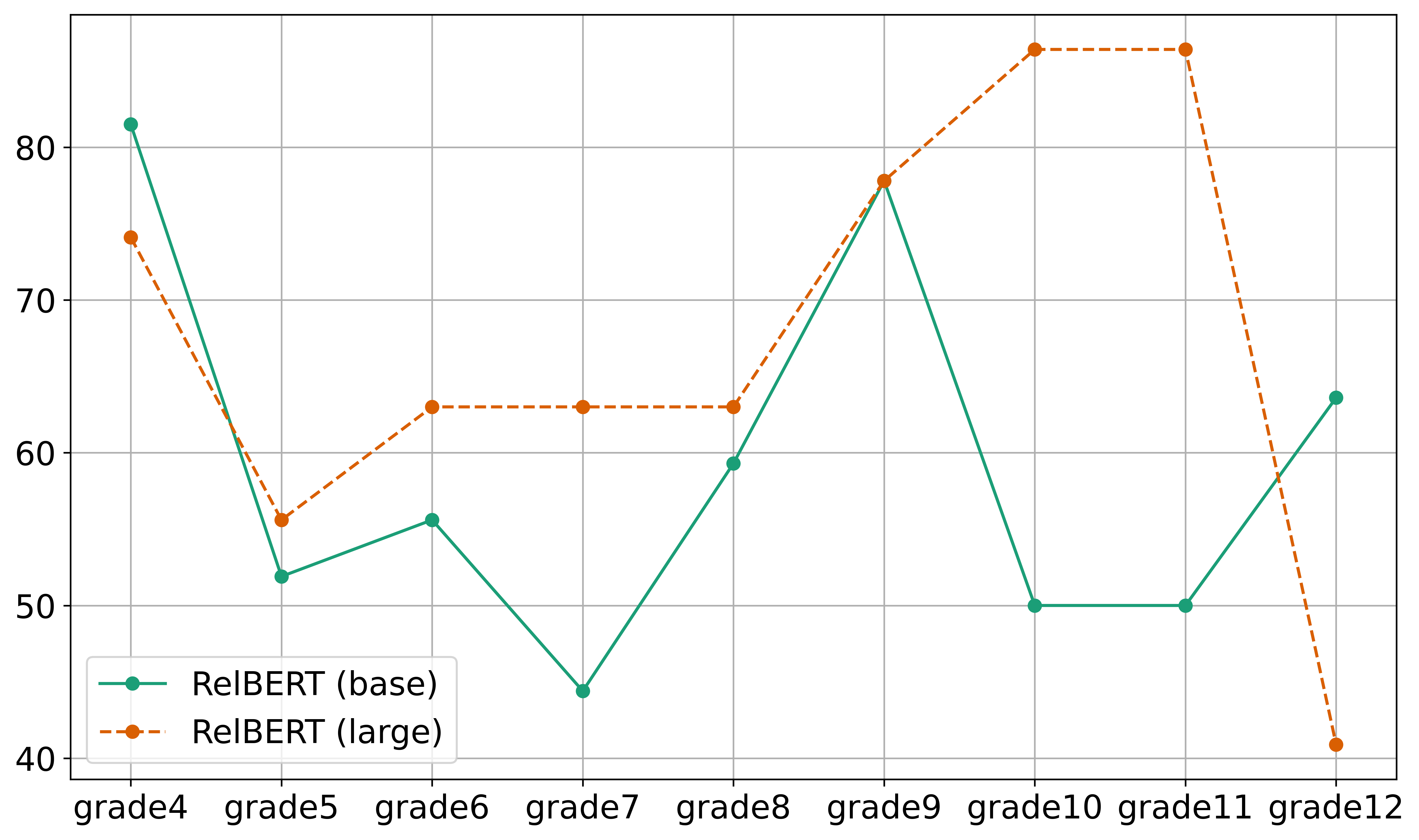
Figure 3: The accuracy of RelBERT for each domain of U2 analogy question.

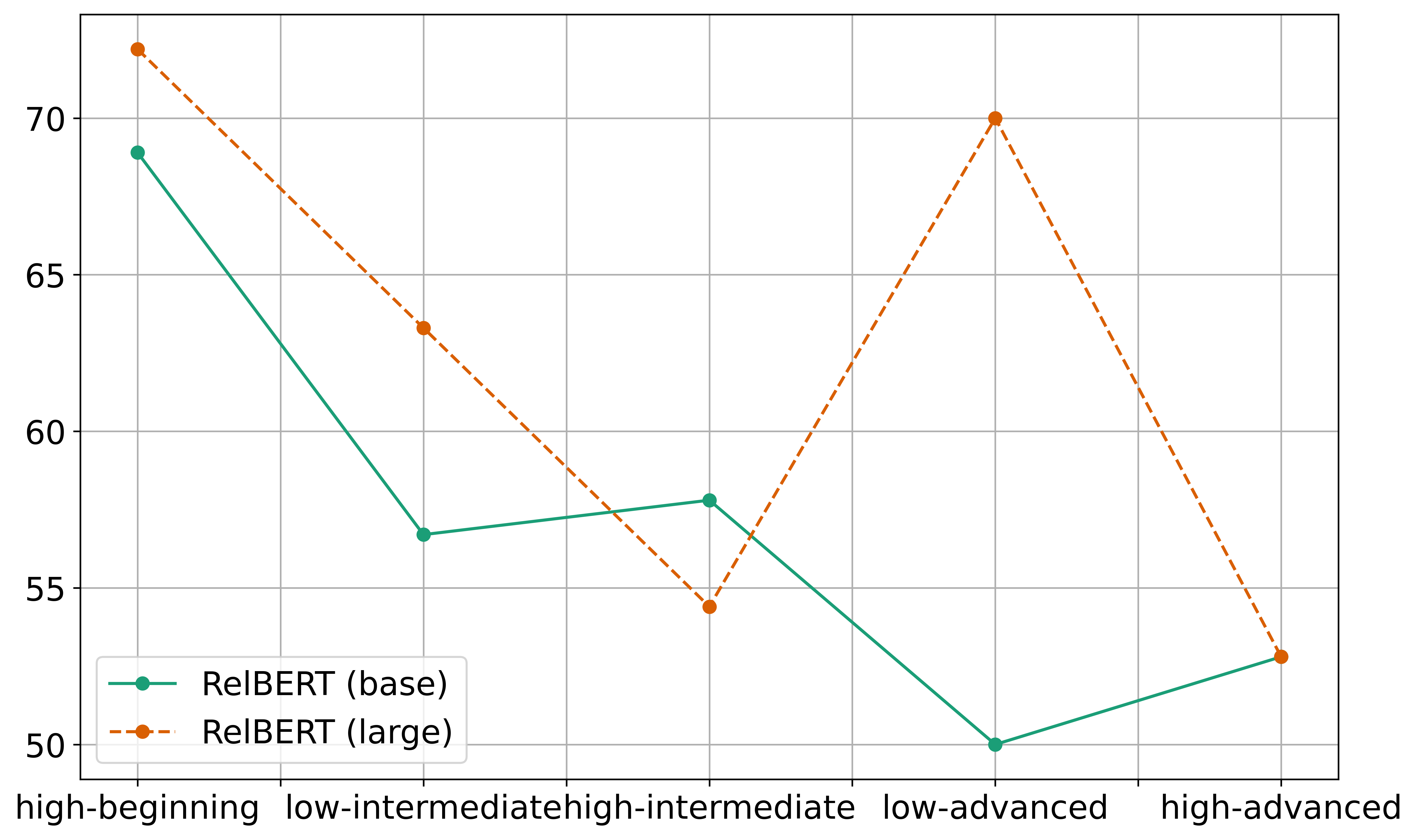
Figure 4: The accuracy of RelBERT for each domain of U4 analogy question.

We now analyse the performance of RelBERT on different categories of analogy questions, considering the categories that were listed in Table 5. First, the results for some of the categories are shown in Table 9, along with some baselines. The results show that both RelBERT models can achieve a high accuracy for morphological relationships, despite not being explicitly trained on such relations. This ability appears to increase along with the model size, as RelBERT_LARGE outperforms RelBERT_BASE by around 10 percentage points on the morphological relations from BATS, and 6 percentage points on the morphological relations from Google. Figure 3 and Figure 4 show the accuracy along with the difficulty level in U2 and U4. Although we cannot see a clear signal in U2, we can see that models struggle more when the difficulty level is increased in U4, especially for RelBERT_BASE. Note that the U2 test is designed for children, while U4 is for college students. As comparison systems, we included the accuracy breakdown of fastText as a word embedding baseline, and Flan-UL2 as the best LM baseline. RelBERT_LARGE consistently outperforms Flan-UL2 in all cases. The performance of fastText is more inconsistent, showing a strong performance on the morphological relations of the Google analogy dataset, as well as the encyclopedic portion of BATS, but performing poorly in the lexical portion of BATS (34.0 compared to RelBERT_Large’s 72.4) and in the metaphors of SCAN (18.9 compared to 24.8).

§ 6.2 Lexical Relation Classification

Table 8 shows the micro F1 score for the lexical relation classification datasets. We can see that RelBERT_LARGE is in general competitive with the SotA approaches. For two (EVALution and ROOT09) out of the four lexical relation classification datasets that have SotA results, RelBERT_LARGE achieves the best results. Moreover, for these two datasets, even RelBERT_BASE outperforms the SotA methods. In terms of reproducible word and pair embedding baselines, RelBERT_LARGE provides better results in all datasets except for BLESS (word embeddings) and K&H+N (pair2vec). We see a consistent improvement in accuracy when going from RelBERT_BASE to RelBERT_LARGE.

§ 7 Analysis

In this section, we analyse the capability of RelBERT from different aspects. We investigate the generalisation ability of RelBERT for unseen relations in § 7.1. In § 7.2, we compare RelBERT with conversational LMs and few-shot learning. Then, we analyse the effect of different design choices in the model architecture in § 7.3. Finally, in § 7.4 we present a qualitative analysis, where among others we show a visualization of the latent representation space of relation vectors.

§ 7.1 Generalization Ability of RelBERT

Dataset\Excluded Relation	Antonym	Attribute	Hypernym	Meronym	Synonym	Full
BLESS
- Attribute	91.6	90.7	90.6	91.6	90.9	91.5
- Co-hyponym	94.6	95.3	95.5	94.0	93.8	93.5
- Event	84.1	84.2	84.0	82.2	84.1	83.6
- Hypernym	92.6	93.5	93.5	91.3	93.1	93.1
- Meronym	85.7	86.8	87.5	85.3	86.7	85.0
- Random	92.1	92.5	92.1	91.7	91.6	91.9
- Average (macro)	90.1	90.5	90.5	89.3	90.0	89.8
- Average (micro)	90.6	90.9	90.8	89.9	90.3	90.2
CogALexV
- Antonym	60.5	64.0	62.9	67.9	63.3	68.2
- Hypernym	56.6	55.5	56.2	56.7	56.4	59.3
- Meronym	70.3	69.5	65.4	70.3	70.5	64.5
- Random	91.9	92.7	92.3	93.2	91.6	92.4
- Synonym	39.0	44.0	42.5	44.4	42.2	45.4
- Average (macro)	63.7	65.1	63.9	66.5	64.8	66.0
- Average (micro)	82.4	83.5	83.0	84.2	82.7	83.7
EVALution
- Attribute	80.7	81.7	80.4	80.3	81.6	82.7
- Antonym	72.0	74.3	73.3	75.2	73.8	73.6
- Hypernym	57.7	59.3	58.5	60.3	59.1	57.5
- Meronym	68.3	71.6	69.0	64.5	66.9	68.8
- Possession	66.7	70.3	66.4	66.0	63.5	67.4
- Synonym	40.6	42.9	37.4	42.9	37.5	41.0
- Average (macro)	63.6	65.7	63.7	64.3	63.0	64.5
- Average (micro)	64.1	65.9	64.3	65.3	63.9	65.0
K&H+N
- Co-hyponym	95.7	96.0	94.2	96.1	94.6	95.1
- Meronym	63.9	63.9	57.7	59.8	62.4	56.7
- Random	96.1	95.9	94.9	96.0	95.3	95.3
- Average (macro)	86.7	86.8	84.0	86.1	85.6	84.5
- Average (micro)	95.0	95.0	93.6	95.1	94.1	94.3
ROOT09
- Co-hyponym	96.9	97.3	96.4	97.3	95.9	95.8
- Hypernym	80.3	80.3	79.0	81.8	79.2	79.5
- Random	89.7	89.7	89.3	89.8	89.0	88.8
- Average (macro)	89.0	89.1	88.2	89.7	88.0	88.0
- Average (micro)	89.2	89.3	88.5	89.7	88.2	88.2

Table 10: F1 score for each relation type of all the lexical relation classification datasets from RelBERT_BASE models fine-tuned on the RelSim without a specific relation. The Full model on the right most column is the original RelBERT_BASE model fine-tuned on full RelSim. The result of the relation type where the model is fine-tuned on RelSim without it, is emphasized by underline.

RelBERT, when trained on RelSim, achieves competitive results on named entities (i.e. Nell-One and T-REX), despite the fact that RelSim does not contain any examples involving named entities. This is one of the most interesting aspects of RelBERT, as it shows that the model learns to infer the relation based on the knowledge from the LM, instead of memorizing the word pairs from the training set. To understand the generalisation ability of RelBERT in more depth, we conduct an additional experiment, where we explicitly exclude a specific relation from RelSim when training RelBERT. Specifically, we train RelBERT on a number of variants of RelSim, where each time a different relation type is excluded. We then test the resulting model on the lexical relation classification datasets. We focus this analysis on the Antonym, Attribute, Hypernym, Meronym, and Synonym relations, as they are covered by both RelSim (see Table 3) and at least one of the lexical relation classification datasets (see Table 6). We train RelBERT_BASE with InfoNCE on the different RelSim variants. Table 10 shows the results. It can be observed that the performance reduces by at most a few percentage points after removing a given target relation. In some cases, we can even see that the results improve after the removal. Hypernym is covered by all the datasets except K&H+N, and the largest decrease can be seen for CogALexV, which is around 3 percentage points. Meronym is covered by all the datasets except ROOT09. After removing the Meronym relation from the training data, the F1 score on meronym prediction increases in three out of four datasets. A similar pattern can be observed for the synonym relation, where the model that was trained without the synonym relation achieves better results than the model trained on the full RelSim dataset. On the other hand, for antonym and attribute, we can see that removing these relations from the training data leads to somewhat lower results on these relations. The average F1 scores over all the relation types are also competitive with, and often even better than those for the full model. These results clearly support the idea that RelBERT can generalise beyond the relation types it is trained on.

§ 7.2 Additional Baselines

We now analyse the performance of two types of additional models: the conversational LMs from OpenAI in § 7.2.1 and models that rely on few-shot demonstrations in § 7.2.2.

§ 7.2.1 ChatGPT and GPT-4

	ChatGPT	GPT-4
Prompt 1	34.7	62.5
Prompt 2	45.7	79.6

Table 11: The accuracy on SAT analogy question for ChatGPT and GPT-4 with the different prompts.

GPT-4 and ChatGPT are two conversational LMs released by OpenAI. As for GPT-3, these models are private and can only be accessed through the OpenAI API. Unlike GPT-3 however, we cannot obtain perplexity scores (or raw model output that would allow us to compute perplexity) through the API. Therefore, we instead ask those models directly to choose the best answer candidate, using the following two text prompts:

1. Answer the question by choosing the correct option. Which of the following is an analogy?
   1) A is to B what C₁ is to D₁
   2) A is to B what C₂ is to D₂
   3) A is to B what C₃ is to D₃
   …
   $\kappa$) A is to B what C_κ is to D_κ
   The answer is

2. Only one of the following statements is correct. Please answer by choosing the correct option.
   1) The relation between A and B is analogous to the relation between C₁ and D₁
   2) The relation between A and B is analogous to the relation between C₂ and D₂
   3) The relation between A and B is analogous to the relation between C₃ and D₃
   …
   ${\kappa}$) The relation between A and B is analogous to the relation between C_κ and D_κ
   The answer is

where (A,B) is the query word pair, and $[C_{i},D_{i}]_{i=1,\dots,\kappa}$ are the candidate word pairs. We manually parse the outputs returned by the model. As GPT-4 is the most expensive endpoint at the moment, we only report the accuracy on the SAT analogy question dataset. Table 11 shows the result, and we can see that GPT-4 achieves state-of-the-art results with one of the prompts, with ChatGPT being considerably worse. However, the gap between two prompts is more than 15 percentage points, which shows that choosing the right prompt is critical when using GPT-4.

§ 7.2.2 Few-shot Learning

Random Seed	0	1	2	3	4	Average
1-shot	44.4	44.7	40.1	48.4	46.0	44.7
5-shots	46.0	47.1	39.8	44.9	49.5	45.5
10-shots	45.7	48.9	33.7	39.6	45.5	42.7

Table 12: The accuracy of [1, 5, 10]-shots learning with five different random seeds.

In the main experiment (§ 6), we used the LM baselines in a zero-shot setting. However, recent LLMs often perform better when a few examples are provided as part of the input [16, 28]. The idea is to provide a few (input,output) pairs at the start of the prompt, followed by the target input. This strategy is commonly referred to as few-shot learning or in-context learning. It is most effective for larger LMs, which can recognize the pattern in the (input,output) pairs and apply this pattern to the target input [28, 26, 27]. Since RelBERT is fine-tuned on RelSim, for this experiment we provide example pairs to the LM input which are taken from RelSim as well.

We focus on the SAT benchmark and the Flan-T5_XXL model, which was the best-performing LM on SAT in the main experiments. We consider [1, 5, 10]-shot learning. The demonstrations in each experiment are randomly chosen from the training split of RelSim. We use the same template as for the zero-shot learning, both to describe the examples and to specify the target input. For example, in the 5-shot learning setting, a complete input to the model with five demonstrations of $[\hat{A}_{i},\hat{B}_{i},\hat{C}_{i},\hat{D}_{i}]_{i=1\dots 5}$ and the target query of $[A,B]$ is shown as below.

$\hat{A}_{1}$ is to $\hat{B}_{1}$ what $\hat{C}_{1}$ is to $\hat{D}_{1}$
$\hat{A}_{2}$ is to $\hat{B}_{2}$ what $\hat{C}_{2}$ is to $\hat{D}_{2}$
$\hat{A}_{3}$ is to $\hat{B}_{3}$ what $\hat{C}_{3}$ is to $\hat{D}_{3}$
$\hat{A}_{4}$ is to $\hat{B}_{4}$ what $\hat{C}_{4}$ is to $\hat{D}_{4}$
$\hat{A}_{5}$ is to $\hat{B}_{5}$ what $\hat{C}_{5}$ is to $\hat{D}_{5}$
A is to B what

We run each experiment for five different random seeds (i.e. five different few-shot prompts for each setting). Table 12 shows the results. Somewhat surprisingly, the few-shot models consistently perform worse than the zero-shot model, which achieved an accuracy of 52.4 in the main experiment.

§ 7.2.3 Multiple-choice Prompt

	Flan-T5XXL	Flan-UL2	OPT-IML30B	OPT-IMLM-30B
Analogical Statement	52.4	50.0	48.9	48.9
Multi-choice QA	35.8	40.6	27.3	31.3

Table 13: The accuracy with multiple-choice prompting compared to the vanilla prompting strategy with the analogical statement ($A$ is to $B$ what $C$ is to $D$) on SAT.

In our main experiment, we compute perplexity separately on each candidate, but the task can be formatted using a multiple-choice question answering prompt as well. Such a prompt provides more information to the LMs, but it requires them to understand the question properly. Following a typical template to solve multiple-choice question answering in the zero-shot setting [16, 28], we use the following text prompt

Which of the following is an analogy?
1) A is to B what C₁ is to D₁
2) A is to B what C₂ is to D₂
3) A is to B what C₃ is to D₃
…
$\kappa$) A is to B what C_κ is to D_κ
The answer is

where (A,B) is the query word pair, and $[C_{i},D_{i}]_{i=1,\dots,\kappa}$ are the candidate word pairs. Table 13 shows the accuracy on SAT, for the four best performing LMs on SAT in the main experiment. We can see that the multiple-choice prompt is substantially worse for all the LMs.

§ 7.3 Ablation Analysis

In this section, we analyse how the performance of RelBERT depends on different design choices that were made. We look at the impact of the training dataset in § 7.3.1; the loss function in § 7.3.2; the number of negative samples for the InfoNCE loss in § 7.3.3; the base language model in § 7.3.4; the prompt templates in § 7.3.5; and the impact of random variations in § 7.3.6. Throughout this section, we use RoBERTa_BASE for efficiency.

§ 7.3.1 The Choice of Datasets

Dataset	RelSim	NELL	T-REX	ConceptNet
Analogy Question
SAT	59.9	36.1	46.8	44.9
U2	59.6	39.9	42.5	42.5
U4	57.4	41.0	44.0	41.0
BATS	70.3	45.5	51.0	62.0
Google	89.2	67.8	75.0	81.0
SCAN	25.9	14.9	19.6	21.8
NELL	62.0	82.5	72.2	66.2
T-REX	66.7	69.9	83.6	44.8
ConceptNet	39.8	10.3	18.8	22.7
Average	59.0	45.3	50.4	47.4
Lexical Relation Classification
BLESS	90.0	88.6	89.3	88.8
CogALexV	83.7	78.6	82.8	82.8
EVALution	64.2	58.7	64.7	62.8
K&H+N	94.0	94.8	95.2	95.0
ROOT09	88.2	86.6	88.2	88.8
Average	84.0	81.5	84.1	83.6

Table 14: The results on analogy questions (accuracy) and lexical relation classification (micro F1 score) of RelBERT with different training datasets, where the best result across models in each dataset are shown in bold.

RelSim is relatively small and does not cover named entities, although the RelBERT model trained on RelSim still performed the best on T-REX and NELL-One in the main experiments. Here we present a comparison with a number of alternative training sets, to see whether better results might be possible. We are primarily interested to see whether the performance on NELL and T-REX might be improved by training RelBERT on the training splits of these datasets. We fine-tune RoBERTa_BASE on three datasets introduced in § 3.3: NELL-One, T-REX and ConceptNet. We use InfoNCE in each case. The results are summarised in Table 14. We can see that training RelBERT on RelSim leads to the best results on most datasets, and the best result on average by a large margin. This is despite the fact that RelSim is significantly smaller than the other datasets (see Table 2). It is particularly noteworthy that training on RelSim outperforms training on ConceptNet even on the ConceptNet test set, even though ConceptNet contains several relation types that are not covered by RelSim. However, when it comes to the relationships between named entities, and the NELL and T-REX benchmarks in particular, training on RelSim underperforms training on NELL or T-REX.

§ 7.3.2 The Choice of Loss Function

Dataset	Triplet	InfoNCE	InfoLOOB
Analogy Question
SAT	54.5	59.9	58.8
U2	55.3	59.6	57.5
U4	58.6	57.4	56.3
BATS	72.6	70.3	67.6
Google	86.4	89.2	83.8
SCAN	29.5	25.9	27.0
NELL	70.7	62.0	67.5
T-REX	45.4	66.7	65.6
ConceptNet	29.4	39.8	40.0
Average	55.8	59.0	58.2
Lexical Relation Classification
BLESS	88.7	90.0	91.0
CogALexV	80.5	83.7	83.3
EVALution	67.7	64.2	65.8
K&H+N	93.1	94.0	94.9
ROOT09	90.3	88.2	89.3
Average	84.1	84.0	84.9

Table 15: The results on analogy questions (accuracy) and lexical relation classification (micro F1 score) with different loss functions, where the best result in each dataset is shown in bold.

In this section, we compare the performance of three different loss functions for training RelBERT. In particular, we fine-tune RoBERTa_BASE on RelSim, and we consider the triplet loss and InfoLOOB, in addition to InfoNCE (see § 3.2 for more in detail). Table 15 shows the result of RelBERT fine-tuned with each of the loss functions. We can see that none of the loss functions consistently outperforms the other. On average, InfoNCE achieves the best results on the analogy questions. The difference with InfoLOOB is small, which is to be expected given that InfoNCE and InfoLOOB are closely related. While the triplet loss performs worse on average, it still manages to achieve the best results in four out of nine analogy datasets. For the relation classification experiments, the results are much closer, with InfoNCE now performing slightly worse than the other loss functions.

§ 7.3.3 The Choice of the Number of Negative Samples

Batch Size	25	50	100	150	200	250	300	350	400	450	500
Analogy Question
SAT	56.1	59.1	53.2	55.6	56.4	57.2	57.5	58.3	59.9	57.2	57.2
U2	55.3	56.1	46.1	53.9	56.1	60.1	56.1	56.6	59.6	59.6	55.7
U4	56.5	57.4	52.5	54.9	57.2	59.0	57.2	54.2	57.4	58.3	56.5
BATS	71.7	69.6	66.9	72.3	69.7	70.9	72.0	73.7	70.3	69.2	70.8
Google	88.2	87.4	78.6	88.0	90.2	89.6	86.4	86.2	89.2	86.6	89.8
SCAN	25.0	27.2	26.2	30.9	26.5	25.3	28.8	31.6	25.9	25.7	25.1
NELL	67.0	66.5	71.5	77.7	66.0	63.7	75.0	77.7	62.0	62.8	63.5
T-REX	59.6	60.7	57.9	57.9	62.3	60.1	57.9	60.1	66.7	69.4	62.8
ConceptNet	36.9	39.3	31.1	29.4	40.5	39.6	31.0	31.4	39.8	38.9	42.8
Average	57.4	58.1	53.8	57.8	58.3	58.4	58.0	58.9	59.0	58.6	58.2
Lexical Relation Classification
BLESS	90.3	90.7	90.3	90.6	90.6	89.5	91.3	90.6	89.6	90.4	89.7
CogALexV	66.0	67.9	65.9	62.5	65.2	64.7	65.4	64.4	65.8	65.4	63.6
EVALution	64.8	62.1	65.0	62.9	63.6	64.6	63.8	63.2	62.9	62.8	64.6
K&H+N	86.0	84.8	87.0	87.5	85.3	85.2	85.2	87.2	84.6	85.4	85.1
ROOT09	87.7	88.8	87.7	88.6	89.4	88.8	88.8	88.6	87.9	88.2	88.0
Average	79.0	78.9	79.2	78.4	78.8	78.6	78.9	78.8	78.2	78.4	78.2

Table 16: The results on analogy questions (accuracy) and lexical relation classification (micro F1 score) with different batch size (negative samples) at InfoNCE, where the best result across models in each dataset is shown in bold.

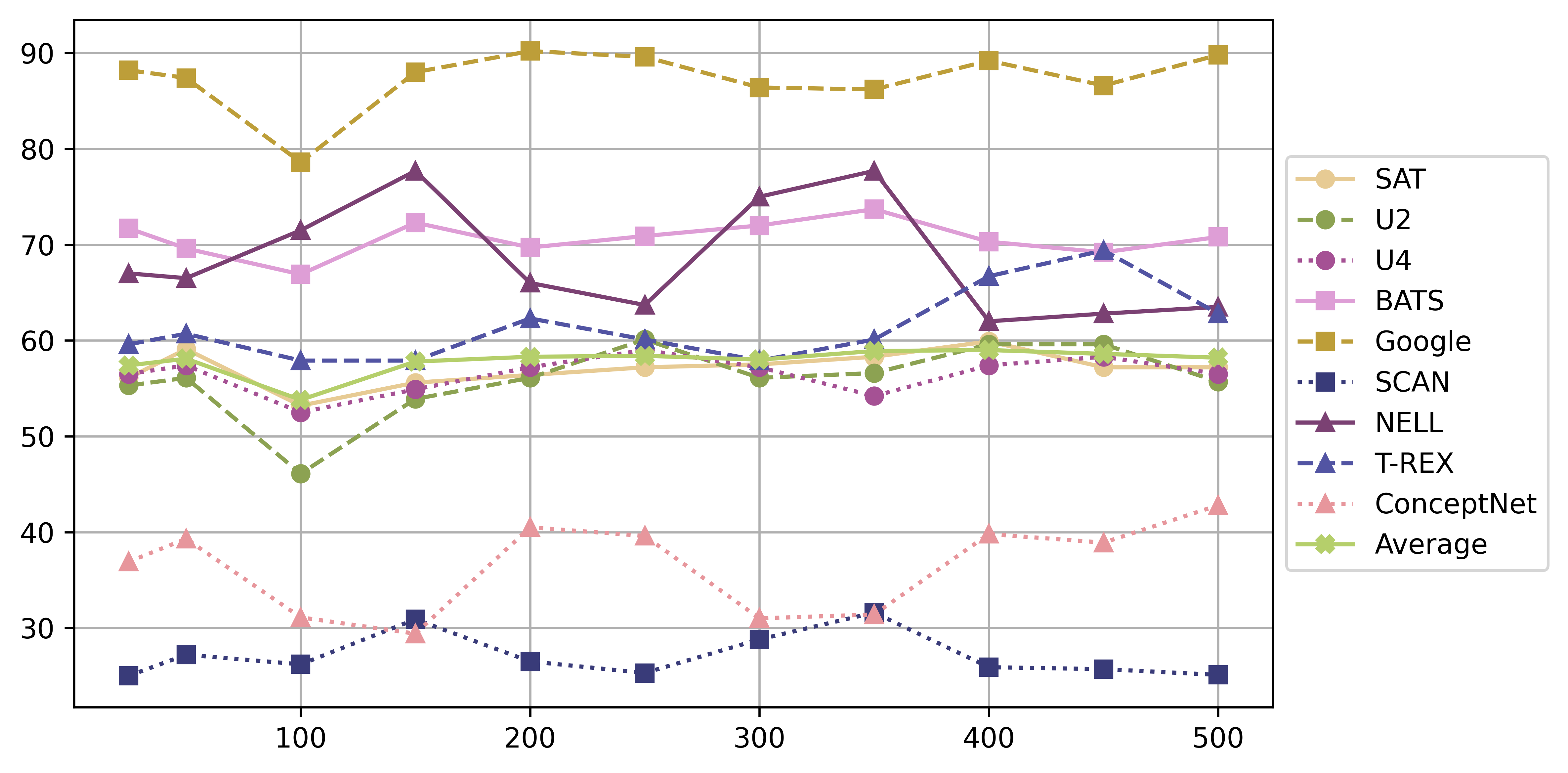
Figure 5: The results on analogy questions in function of the batch size.

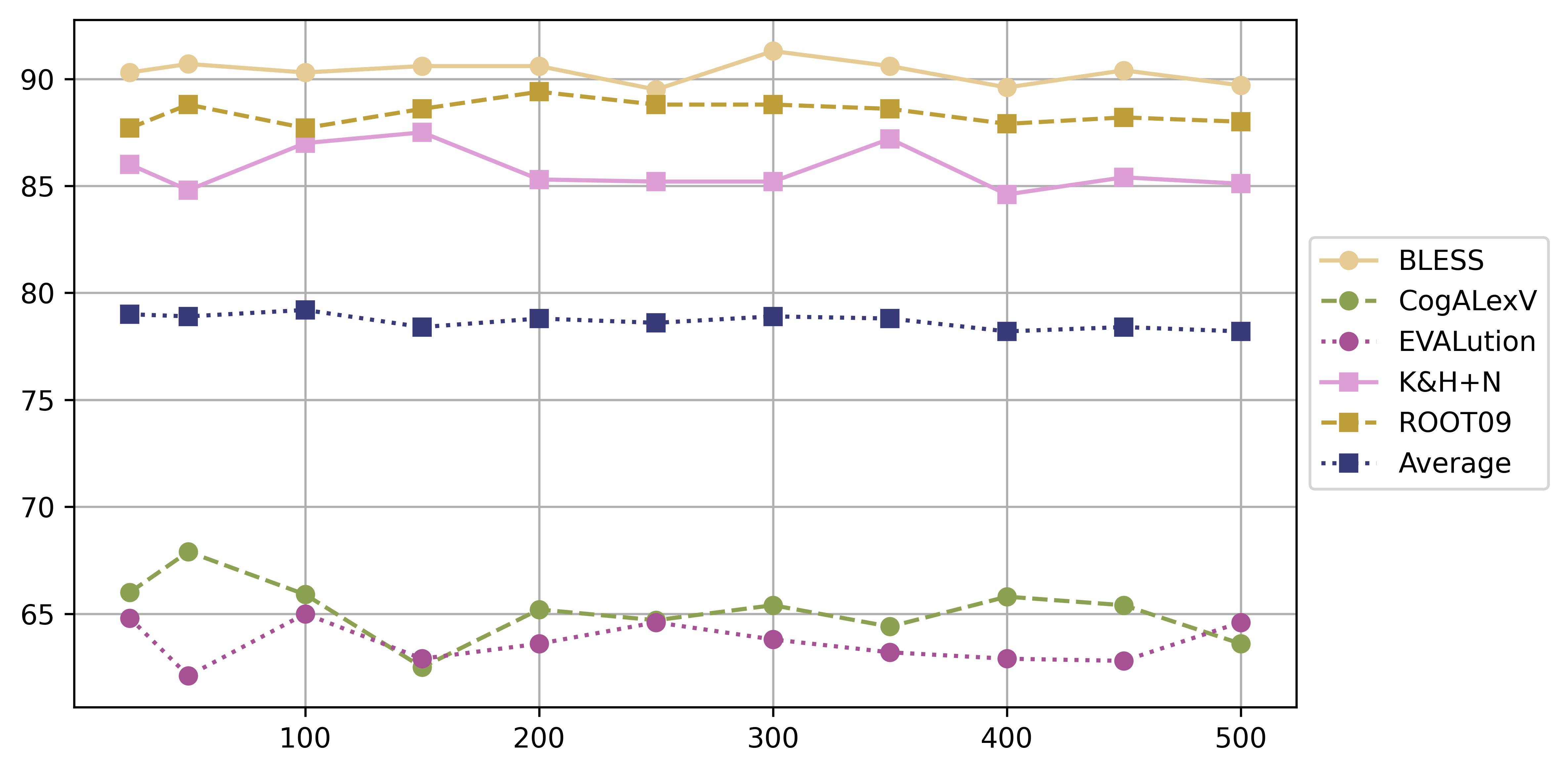
Figure 6: The results on lexical relation classification in function of the batch size.

The variant of InfoNCE that we considered for training RelBERT relies on in-batch negative samples, i.e. the negative samples for a given anchor pair correspond to the other word pairs that are included in the same batch. The number of negative samples that are considered thus depends on the batch size. In general, using a larger number of negative samples tends to benefit contrastive learning strategies, but it comes at the price of an increase in memory requirement. Here we analyse the impact of this choice, by comparing the results we obtained for different batch sizes. We train RelBERT_BASE on RelSim with batch sizes from [25, 50, 100, 150, 200, 250, 300, 350, 400, 450, 500], where the batch size 400 corresponds to our main RelBERT_BASE model. The results are shown in Table 16, and visually illustrated in Figure 5 and Figure 6. Somewhat surprisingly, the correlation between batch size and performance is very weak. For analogy questions, there is a weak positive correlation. The Spearman $\rho$ correlation to the batch size for T-REX is 0.6 with p-value 0.047, but in other datasets, correlations are not significant (i.e. p-values are higher than 0.05). Indeed, even a batch size of 25 is sufficient to achieve close-to-optimal results. For lexical relation classification, the Spearman correlation is not significant for any of the datasets.

§ 7.3.4 The Choice of Language Model

	BERTBASE	ALBERTBASE	RoBERTaBASE
Analogy Question
SAT	44.7	40.4	59.9
U2	36.8	35.5	59.6
U4	40.0	38.7	57.4
BATS	54.9	59.2	70.3
Google	72.2	56.4	89.2
SCAN	23.7	21.2	25.9
NELL	56.7	47.7	62.0
T-REX	49.2	32.8	66.7
ConceptNet	27.1	25.7	39.8
Average	45.0	39.7	59.0
Lexical Relation Classification
BLESS	90.9	88.0	90.0
CogALexV	80.7	78.3	83.7
EVALution	61.8	58.1	64.2
K&H+N	95.5	92.9	94.0
ROOT09	88.7	85.6	88.2
Average	83.5	80.6	84.0

Table 17: The results on analogy questions (accuracy) and lexical relation classification (micro F1 score) of RelBERT with different LMs, where the best results across models in each dataset are shown in bold.

Thus far, we have only considered RoBERTa as the base language model for training RelBERT. Here we compare RoBERTa with two alternative choices: BERT [15] and ALBERT [128]. We compare BERT_BASE, ALBERT_BASE, and RoBERTa_BASE, fine-tuned on RelSim with InfoNCE. Table 17 shows the result. RoBERTa_BASE is found to consistently achieve the best results on analogy questions, with a surprisingly large margin. RoBERTa_BASE also achieved the best result, on average, for lexical relation classification, although in this case it only achieves the best results in two out of five datasets. ALBERT consistently has the worst performance, struggling even on the relatively easy Google dataset. These results clearly show that the choice of the LM is of critical importance for the performance of RelBERT.

§ 7.3.5 The Choice of Prompt Template

Our main experiment relies on the five prompt templates introduced in § 3.1, where we choose the best among these five templates based on the validation loss. We now analyse the impact of these prompt templates. We focus this analysis on RelBERT_BASE, i.e. RoBERTa_BASE fine-tuned with InfoNCE on RelSim. For this configuration, the template that was selected based on validation accuracy is

Today, I finally discovered the relation between [h] and [t] : [h] is the <mask> of [t]

We experiment with a number of variations of this template. First, we will see whether the length of the template plays an important role, and in particular whether a similar performance can be achieved with shorter templates. Subsequently we also analyse to what extent the wording of the template matters, i.e. whether similar results are possible with templates that are less semantically informative.

The Effect of Length

Template	A (Original)	B	C	D	E
Analogy Question
SAT	59.9	58.3	56.7	59.4	46.3
U2	59.6	57.9	57.9	56.6	44.7
U4	57.4	57.6	54.9	60.0	46.8
BATS	70.3	69.6	70.0	73.9	65.6
Google	89.2	88.0	89.4	93.4	81.8
SCAN	25.9	24.8	23.9	27.1	25.2
NELL	62.0	65.5	64.2	65.5	59.2
T-REX	66.7	62.3	60.1	56.8	48.1
ConceptNet	39.8	39.0	37.8	39.5	32.4
Average	59.0	59.4	58.8	61.7	51.7
Lexical Relation Classification
BLESS	89.9	89.2	89.2	90.5	88.2
CogALexV	65.7	65.3	66.7	69.6	63.3
EVALution	65.1	64.8	63.1	64.9	63.0
K&H+N	85.3	85.3	83.7	86.2	86.9
ROOT09	89.1	87.6	88.9	89.8	87.8
Average	79.0	78.4	78.3	80.2	77.8

Table 18: The results on analogy questions (accuracy) and lexical relation classification (micro F1 score) of RelBERT fine-tuned with different length of templates, where the best results across models in each dataset are shown in bold.

Phrase	the	Napoleon	football	Italy	Cardiff	the earth	pizza	subway	ocean	Abraham	the
	spaceship	Bonaparte				science				Lincoln	relation
Analogy Question
SAT	57.2	56.7	56.1	58.0	57.2	59.6	57.0	59.6	56.7	59.9	59.9
U2	55.3	58.3	56.6	55.3	57.5	58.3	55.7	57.0	57.5	56.1	59.6
U4	56.9	58.1	56.5	56.2	55.1	56.9	56.7	55.3	55.8	57.2	57.4
BATS	71.2	69.1	69.5	68.8	69.5	69.9	68.5	69.8	68.9	69.5	70.3
Google	87.2	85.4	87.6	85.2	86.8	89.2	85.6	87.6	86.0	89.2	89.2
SCAN	25.6	26.8	25.7	26.1	26.2	22.6	25.8	26.6	25.6	24.6	25.9
NELL	64.8	61.7	63.8	63.5	60.0	64.7	65.8	63.3	63.3	66.2	62.0
T-REX	63.4	51.9	57.4	59.6	55.7	56.3	59.0	60.1	60.7	60.7	66.7
ConceptNet	39.6	39.4	38.5	36.9	37.9	39.3	38.5	38.8	38.8	38.3	39.8
Average	57.9	56.4	56.9	56.6	56.2	57.4	57.0	57.6	57.0	58.0	59.0
Lexical Relation Classification
BLESS	89.9	89.7	90.0	90.0	89.2	91.4	89.7	89.7	90.6	89.3	89.9
CogALexV	63.4	64.7	66.5	65.7	66.3	65.3	66.0	65.3	65.3	64.1	65.7
EVALution	63.6	63.7	64.0	63.8	62.4	63.5	64.5	63.3	63.5	64.0	65.1
K&H+N	84.8	86.2	86.4	85.9	85.3	84.8	84.7	84.6	85.1	85.0	85.3
ROOT09	88.5	88.9	89.4	89.0	89.2	88.7	89.1	89.5	88.9	89.6	89.1
Average	78.0	78.6	79.3	78.9	78.5	78.7	78.8	78.5	78.7	78.4	79.0

Table 19: The results on analogy questions (accuracy) and lexical relation classification (micro F1 score) of RelBERT fine-tuned with random phrase to construct the template, where the best results across models in each dataset are shown in bold.

We start from the best template chosen for RelBERT_BASE, and shorten it while preserving its meaning as much as possible. Specifically, we considered the following variants:

1. Today, I finally discovered the relation between [h] and [t] : [h] is the <mask> of [t]

2. I discovered the relation between [h] and [t]: [h] is the <mask> of [t]

3. the relation between [h] and [t]: [h] is the <mask> of [t]

4. I discovered: [h] is the <mask> of [t]

5. [h] is the <mask> of [t]

For each of the templates, we fine-tune RoBERTa_BASE with InfoNCE on RelSim. The results are summarised in Table 18. We find that template D outperforms the original template A on average, both for analogy questions and for lexical relation classification. In general, we thus find no clear link between the length of the template and the resulting performance, although the shortest template (template E) achieves by far the worst results. This suggests that, while longer templates are not necessarily better, using templates which are too short may be problematic.

The Effect of Semantics

We now consider variants of the original template in which the anchor phrase “the relation” is replaced by a semantically meaningful distractor, i.e. we consider templates of the following form:

Today, I finally discovered <semantic phrase> between [h] and [t] : [h] is the <mask> of [t]

where <semantic phrase> is a placeholder for the chosen anchor phrase. We randomly chose 10 phrases (four named entities and six nouns) to play the role of this anchor phrase. For each of the resulting templates, we fine-tune RoBERTa_BASE with InfoNCE on the RelSim dataset. Table 19 shows the result. We can see that the best results are obtained with the original template, both for analogy questions and for lexical relation classification. Nevertheless, the difference in performance is surprisingly limited. The largest decrease is 2.8 in the average for analogy questions and 1.0 in the average for lexical relation classification, which is smaller than the differences we observed when using the shortest template, or when changing the LM § 7.3.4 or the loss function § 7.3.2.

§ 7.3.6 The Choice of Random Seed

	RelBERTBASE				RelBERTLARGE
Random Seed	0	1	2	Average	0	1	2	Average
Analogy Question
SAT	59.9	54.3	55.9	56.7 $\pm$2.9	68.2	68.4	71.9	69.5 $\pm$2.1
U2	59.6	51.8	55.7	55.7 $\pm$3.9	67.5	65.4	68.0	67.0 $\pm$1.4
U4	57.4	53.7	54.4	55.2 $\pm$2.0	63.9	65.0	66.4	65.1 $\pm$1.3
BATS	70.3	65.3	67.3	67.6 $\pm$2.5	78.3	79.7	80.4	79.5 $\pm$1.1
Google	89.2	79.4	85.6	84.7 $\pm$5.0	93.4	93.4	94.8	93.9 $\pm$0.8
SCAN	25.9	25.9	23.3	25.1 $\pm$1.5	25.9	27.0	29.1	27.4 $\pm$1.6
NELL	62.0	71.0	63.5	65.5 $\pm$4.8	60.5	67.3	66.3	64.7 $\pm$3.7
T-REX	66.7	55.2	46.4	56.1 $\pm$10.1	67.8	65.0	63.4	65.4 $\pm$2.2
ConceptNet	39.8	27.4	30.5	32.6 $\pm$6.4	43.3	44.8	48.7	45.6 $\pm$2.8
Average	59.0	53.8	53.6	55.5 $\pm$3.1	63.2	64.0	65.4	64.2 $\pm$1.1
Lexical Relation Classification
BLESS	90.0	91.4	90.7	90.7 $\pm$0.7	91.5	92.4	91.7	91.9 $\pm$0.5
CogALexV	83.7	81.5	81.1	82.1 $\pm$1.4	84.9	86.5	86.4	85.9 $\pm$0.9
EVALution	64.2	63.3	63.1	63.5 $\pm$0.6	66.9	69.0	67.8	67.9 $\pm$1.0
K&H+N	94.0	94.7	94.3	94.3 $\pm$0.4	95.1	95.3	95.7	95.3 $\pm$0.3
ROOT09	88.2	88.3	89.5	88.7 $\pm$0.7	89.2	89.5	91.5	90.1 $\pm$1.3
Average	84.0	83.8	83.7	83.9 $\pm$0.1	85.5	86.5	86.6	86.2 $\pm$0.6

Table 20: Result of RelBERT_BASE and RelBERT_LARGE with three runs with different random seed, and the average and the standard deviation in each dataset.

In this section, we investigate the stability of RelBERT training, by comparing the results we obtained for different random seeds. We use a fixed random seed of 0 as default in the main experiments. Here we include results for two other choices of the random seed. We train both of RelBERT_BASE and RelBERT_LARGE. However, different from the main experiments, for this analysis we reduce the batch size from 400 to 100 for RelBERT_LARGE, to reduce the computation time. Table 20 shows the result. We observe that the standard deviation is higher for RelBERT_BASE than for RelBERT_LARGE. For example, the accuracy on T-REX differs from 46.4 to 66.7 for RelBERT_BASE, while only ranging between 63.4 and 67.8 for RelBERT_LARGE. We can also see that there is considerably less variation in performance for lexical relation classification, compared to analogy questions.

§ 7.4 Qualitative Analysis

		AtLocation	CapableOf	IsA
RelBERTLARGE	1	child:school, animal:zoo,	dog:bark, cat:hunt mouse	baseball:sport, sushi:food,
		prisoner:jail, fish:aquarium,	lawyer:settle lawsuit,	yo-yo:toy, dog:mammal,
		librarian:library	pilot:land plane	spanish:language
	2	computer:office, book:shelf,	knife:spread butter,	canada:country,
		coat:closet, food:refrigerator,	clock:tell time, comb:part hair,	california:state,
		paper clip:desk	match:light fire	san francisco:city
RelBERTBASE	1	animal:zoo, elephant:zoo,	dog:bark, student:study,	baseball:sport,
		student:classroom,	ball:bounce, tree:grow,	soccer:sport,
		student:school	bomb:explode	chess:game
	2	computer:office, coat:closet,	plane:fly, clock:tell time,	dog:mammal, rose:flower,
		mirror:bedroom, notebook:desk,	computer:compute,	violin:string instrument,
		food:refrigerator	knife:spread butter	fly:insect, rice:food
fastText	1	fish:water, child:school,	cat:hunt mouse, cat:drink water,
		bookshelf:library, feather:bird,	dog:guide blind person,
		computer:office	dog:guard house
	2	animal:zoo, elephant:zoo,	knife:spread butter,
		lion:zoo, weasel:zoo,	turtle:live long time,
		tiger:zoo	magician:fool audience

Table 21: Examples of word pairs in the clusters obtained by HDBSCAN for different relation embeddings. For the IsA relation, all word pairs were clustered together in the case of fastText.

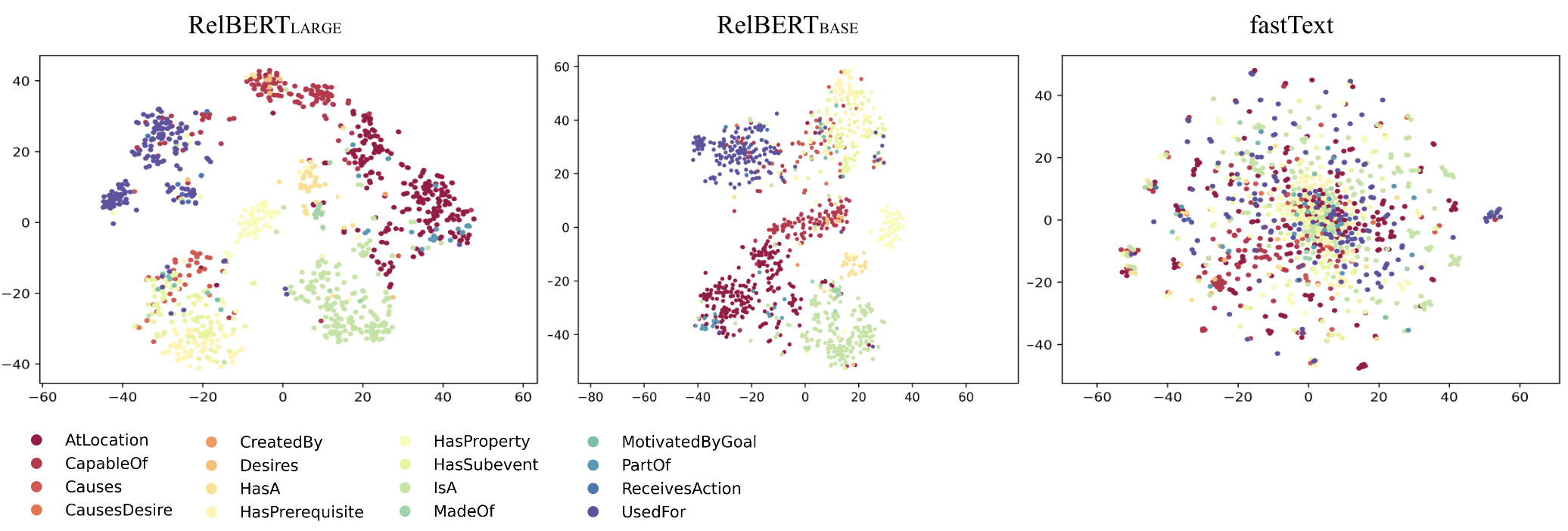
(a) ConceptNet

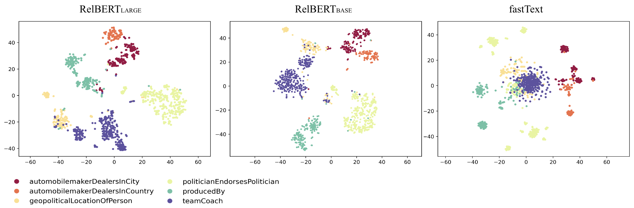
(b) NELL-One

Figure 7: The tSNE 2-dimension visualization of relation embeddings over the test set of (a) ConceptNet and (b) NELL-One. Colours reflect the relation type of the embedded word pairs.

We qualitatively analyse the latent space of the RelBERT relation vectors. For this analysis, we focus on the test splits of the ConceptNet and NELL-One datasets. We compute the relation embeddings of all the word pairs in these datasets using RelBERT_BASE and RelBERT_LARGE. As a comparison, we also compute relation embeddings using fastText, in the same way as in § 5.2. First, we visualize the relation embeddings, using tSNE [129] to map the embeddings to a two-dimensional space. Figure 7 shows the resulting two-dimensional relation embeddings. The plots clearly show how the different relation types are separated much more clearly for RelBERT than for fastText. For ConceptNet, in particular, we can see that the fastText representations are mixed together. Comparing RelBERT_LARGE and RelBERT_BASE, there is no clear difference for NELL-One. For ConceptNet, we can see that RelBERT_LARGE leads to clusters which are somewhat better separated.

Second, we want to analyse whether RelBERT vectors could model relations in a more fine-grained way than existing knowledge graphs. We focus on ConceptNet for this analysis. We cluster the RelBERT vectors of the word pairs in each relation type using HDBSCAN [130]. We focus on three relation types: AtLocation, CapableOf, and IsA. These are the relation types with the highest number of instances, among those for which HDBSCAN yielded more than one cluster. We obtained two clusters for each of these relation types. Table 21 shows some examples of word pairs in each cluster. For AtLocation, RelBERT separates the word pairs depending on whether the head denotes a living thing. On the other hand, fastText captures a surface feature and forms a cluster where the word pairs have “zoo” as tails. All other word pairs are mixed together in the first cluster. For CapableOf, RelBERT_LARGE again distinguishes the word pairs based on whether the head entity denotes a living thing. For RelBERT_BASE, the clusters are not separated as clearly, while fastText again focuses on the presence of particular words such as “cat” and “dog” in this case. For IsA, RelBERT_LARGE yields a cluster that specifically focuses on geolocations. RelBERT_BASE puts pairs with the words “sport” or “game” together. In the case of fastText, all pairs were clustered together. Overall, fastText tends to catch the surface features of the word pairs. RelBERT_LARGE seems to find meaningful distinctions, although at least in these examples, they are focused on the semantic types of the entities involved rather than any specialisation of the relationship itself. The behaviour of RelBERT_BASE is similar, albeit clearly noisier.

§ 8 Conclusion

We have proposed a strategy for learning relation embeddings, i.e. vector representations of pairs of words which capture their relationship. The main idea is to fine-tune a pre-trained language model using a relational similarity dataset covering a broad range of semantic relations. In our experimental results, we found the resulting relation embeddings to be of high quality, outperforming state-of-the-art methods on most analogy questions and relation classification benchmarks, while maintaining the flexibility of an embedding model. Crucially, we found that RelBERT is capable of modelling relationships that go well beyond those that are covered by the training data, including morphological relations and relations between named entities. Being based on RoBERTa_LARGE, our main RelBERT model has 354M parameters. This relatively small size makes RelBERT convenient and efficient to use in practice. Surprisingly, we found RelBERT to significantly outperform language models which are several orders of magnitude larger.

While many NLP tasks can now be solved by prompting LLMs, learning explicit representations remains important for tasks that require transparency or efficiency. For instance, we envision that RelBERT can play an important role in the context of semantic search, e.g. to find relevant context for retrieval augmented LMs [131]. Explicit representations also matter for tasks that cannot easily be described using natural language instructions, such as ontology alignment [132] and completion [133, 134], where relation embeddings should intuitively also be clearly useful. More generally, RelBERT has the potential to improve applications that currently rely on commonsense KGs such as ConceptNet, e.g. commonsense question answering with smaller LMs [29] and scene graph generation [33].

Appendix A Model Names on HuggingFace

Model	Name on HuggingFace
ALBERTBASE	albert-base-v2
BERTBASE	bert-base-cased
BERTLARGE	bert-large-cased
RoBERTaBASE	roberta-base
RoBERTaLARGE	roberta-large
GPT-2SMALL	gpt2
GPT-2BASE	gpt2-medium
GPT-2LARGE	gpt2-large
GPT-2XL	gpt2-xl
GPT-J125M	EleutherAI/gpt-neo-125M
GPT-J1.3B	EleutherAI/gpt-neo-1.3B
GPT-J2.7B	EleutherAI/gpt-neo-2.7B
GPT-J6B	EleutherAI/gpt-j-6B
GPT-J20B	EleutherAI/gpt-neox-20b
OPT125M	facebook/opt-125m
OPT350M	facebook/opt-350m
OPT1.3B	facebook/opt-1.3b
OPT30B	facebook/opt-30b
OPT-IML1.3B	facebook/opt-iml-1.3b
OPT-IML30B	facebook/opt-iml-30b
OPT-IMLM-1.3B	facebook/opt-iml-max-1.3b
OPT-IMLM-30B	facebook/opt-iml-max-30b
T5SMALL	t5-small
T5BASE	t5-base
T5LARGE	t5-large
T53B	t5-3b
T511B	t5-11b
Flan-T5SMALL	google/flan-t5-small
Flan-T5BASE	google/flan-t5-base
Flan-T5LARGE	google/flan-t5-large
Flan-T5XL	google/flan-t5-xl
Flan-T5XXL	google/flan-t5-xxl
Flan-UL2	google/flan-ul2

Table 22: The language models used in the paper and their corresponding alias on HuggingFace model hub.

Table 22 is a list of language models we used in the paper with their names on HuggingFace molde hub, where we take the pre-trained model weight.

Appendix B Hyperparameters of RelBERT

Language Model	Aggregation	Dataset	Loss	Template	Epoch	Seed	Batch
RoBERTaBASE	average w.o. mask	RelSim	InfoNCE	1	8	0	400
RoBERTaBASE	average w.o. mask	RelSim	InfoNCE	5	10	1	400
RoBERTaBASE	average w.o. mask	RelSim	InfoNCE	5	9	2	400
RoBERTaBASE	average w.o. mask	RelSim	InfoNCE	1	10	0	25
RoBERTaBASE	average w.o. mask	RelSim	InfoNCE	1	6	0	50
RoBERTaBASE	average w.o. mask	RelSim	InfoNCE	2	6	0	100
RoBERTaBASE	average w.o. mask	RelSim	InfoNCE	5	8	0	150
RoBERTaBASE	average w.o. mask	RelSim	InfoNCE	1	8	0	200
RoBERTaBASE	average w.o. mask	RelSim	InfoNCE	1	9	0	250
RoBERTaBASE	average w.o. mask	RelSim	InfoNCE	5	10	0	300
RoBERTaBASE	average w.o. mask	RelSim	InfoNCE	5	9	0	350
RoBERTaBASE	average w.o. mask	RelSim	InfoNCE	1	8	0	450
RoBERTaBASE	average w.o. mask	RelSim	InfoNCE	1	9	0	500
RoBERTaLARGE	average w.o. mask	RelSim	InfoNCE	1	8	0	100
RoBERTaLARGE	average w.o. mask	RelSim	InfoNCE	4	9	1	100
RoBERTaLARGE	average w.o. mask	RelSim	InfoNCE	4	8	2	100
RoBERTaLARGE	average w.o. mask	RelSim	InfoNCE	4	9	0	400
RoBERTaBASE	average w.o. mask	RelSim	InfoLOOB	1	4	0	400
RoBERTaBASE	average w.o. mask	RelSim	Triplet	5	1	0	400
RoBERTaBASE	average w.o. mask	NELL	InfoNCE	5	5	0	400
RoBERTaBASE	average w.o. mask	T-REX	InfoNCE	1	4	0	400
RoBERTaBASE	average w.o. mask	ConceptNet	InfoNCE	4	5	0	400
RoBERTaBASE	average w.o. mask	RelSim	InfoNCE	1	8	0	400
BERTBASE	average w.o. mask	RelSim	InfoNCE	1	6	0	400
ALBERTBASE	average w.o. mask	RelSim	InfoNCE	1	5	0	400

Table 23: The best configuration of the template and the number of epoch.

Table 23 shows the best combination of the template and the number of epoch for each of the models used in our paper.

References

- [1] P. D. Turney, Measuring semantic similarity by latent relational analysis, in: Proc. of IJCAI, 2005, pp. 1136–1141.
- [2] D. Lin, P. Pantel, DIRT - discovery of inference rules from text, in: Proceedings of the 7th Iternational Conference on Knowledge Discovery and Data Mining, 2001, pp. 323–328.
- [3] T. Mikolov, I. Sutskever, K. Chen, G. S. Corrado, J. Dean, Distributed Representations of Words and Phrases and their Compositionality, in: Advances in Neural Information Processing Systems, 2013, pp. 3111–3119.
-
[4]
J. Pennington, R. Socher, C. Manning,
GloVe: Global vectors for word
representation, in: Proceedings of the 2014 Conference on Empirical Methods
in Natural Language Processing (EMNLP), Association for Computational
Linguistics, Doha, Qatar, 2014, pp. 1532–1543.
doi:10.3115/v1/D14-1162.
URL https://aclanthology.org/D14-1162 - [5] P. Bojanowski, E. Grave, A. Joulin, T. Mikolov, Enriching word vectors with subword information, arXiv preprint arXiv:1607.04606 (2016).
-
[6]
A. Gladkova, A. Drozd, S. Matsuoka,
Analogy-based detection of
morphological and semantic relations with word embeddings: what works and
what doesn’t., in: Proceedings of the NAACL Student Research Workshop,
Association for Computational Linguistics, San Diego, California, 2016, pp.
8–15.
doi:10.18653/v1/N16-2002.
URL https://aclanthology.org/N16-2002 -
[7]
E. Vylomova, L. Rimell, T. Cohn, T. Baldwin,
Take and took, gaggle and goose,
book and read: Evaluating the utility of vector differences for lexical
relation learning, in: Proceedings of the 54th Annual Meeting of the
Association for Computational Linguistics (Volume 1: Long Papers),
Association for Computational Linguistics, Berlin, Germany, 2016, pp.
1671–1682.
doi:10.18653/v1/P16-1158.
URL https://aclanthology.org/P16-1158 -
[8]
T. Linzen, Issues in evaluating
semantic spaces using word analogies, in: Proceedings of the 1st Workshop on
Evaluating Vector-Space Representations for NLP, Association for
Computational Linguistics, Berlin, Germany, 2016, pp. 13–18.
doi:10.18653/v1/W16-2503.
URL https://aclanthology.org/W16-2503 -
[9]
A. Drozd, A. Gladkova, S. Matsuoka,
Word embeddings, analogies, and
machine learning: Beyond king - man + woman = queen, in: Proceedings of
COLING 2016, the 26th International Conference on Computational
Linguistics: Technical Papers, The COLING 2016 Organizing Committee, Osaka,
Japan, 2016, pp. 3519–3530.
URL https://aclanthology.org/C16-1332 -
[10]
Z. Bouraoui, S. Jameel, S. Schockaert,
Relation induction in word
embeddings revisited, in: Proceedings of the 27th International Conference
on Computational Linguistics, Association for Computational Linguistics,
Santa Fe, New Mexico, USA, 2018, pp. 1627–1637.
URL https://aclanthology.org/C18-1138 - [11] P. D. Turney, M. L. Littman, J. Bigham, V. Shnayder, Combining independent modules in lexical multiple-choice problems, in: Recent Advances in Natural Language Processing III, 2003, pp. 101–110.
-
[12]
A. Ushio, L. Espinosa Anke, S. Schockaert, J. Camacho-Collados,
BERT is to NLP what
AlexNet is to CV: Can pre-trained language models identify analogies?,
in: Proceedings of the 59th Annual Meeting of the Association for
Computational Linguistics and the 11th International Joint Conference on
Natural Language Processing (Volume 1: Long Papers), Association for
Computational Linguistics, Online, 2021, pp. 3609–3624.
doi:10.18653/v1/2021.acl-long.280.
URL https://aclanthology.org/2021.acl-long.280 - [13] D. Vrandečić, M. Krötzsch, Wikidata: a free collaborative knowledgebase, Communications of the ACM 57 (10) (2014) 78–85.
- [14] R. Speer, J. Chin, C. Havasi, Conceptnet 5.5: An open multilingual graph of general knowledge, in: Proceedings of the Thirty-First AAAI Conference on Artificial Intelligence, 2017.
-
[15]
J. Devlin, M.-W. Chang, K. Lee, K. Toutanova,
BERT: Pre-training of deep
bidirectional transformers for language understanding, in: Proceedings of
the 2019 Conference of the North American Chapter of the Association for
Computational Linguistics: Human Language Technologies, Volume 1 (Long and
Short Papers), Association for Computational Linguistics, Minneapolis,
Minnesota, 2019, pp. 4171–4186.
doi:10.18653/v1/N19-1423.
URL https://aclanthology.org/N19-1423 - [16] T. B. Brown, B. Mann, N. Ryder, M. Subbiah, J. Kaplan, P. Dhariwal, A. Neelakantan, P. Shyam, G. Sastry, A. Askell, S. Agarwal, A. Herbert-Voss, G. Krueger, T. Henighan, R. Child, A. Ramesh, D. M. Ziegler, J. Wu, C. Winter, C. Hesse, M. Chen, E. Sigler, M. Litwin, S. Gray, B. Chess, J. Clark, C. Berner, S. McCandlish, A. Radford, I. Sutskever, D. Amodei, Language models are few-shot learners, in: Proceedings of the Annual Conference on Neural Information Processing Systems, 2020.
-
[17]
C. Raffel, N. Shazeer, A. Roberts, K. Lee, S. Narang, M. Matena, Y. Zhou,
W. Li, P. J. Liu, Exploring the
limits of transfer learning with a unified text-to-text transformer, Journal
of Machine Learning Research 21 (140) (2020) 1–67.
URL http://jmlr.org/papers/v21/20-074.html -
[18]
F. Petroni, T. Rocktäschel, S. Riedel, P. Lewis, A. Bakhtin, Y. Wu,
A. Miller, Language models as
knowledge bases?, in: Proceedings of the 2019 Conference on Empirical
Methods in Natural Language Processing and the 9th International Joint
Conference on Natural Language Processing (EMNLP-IJCNLP), Association for
Computational Linguistics, Hong Kong, China, 2019, pp. 2463–2473.
doi:10.18653/v1/D19-1250.
URL https://aclanthology.org/D19-1250 -
[19]
Z. Jiang, F. F. Xu, J. Araki, G. Neubig,
How can we know what language
models know?, Transactions of the Association for Computational Linguistics
8 (2020) 423–438.
doi:10.1162/tacl_a_00324.
URL https://aclanthology.org/2020.tacl-1.28 -
[20]
B. Heinzerling, K. Inui,
Language models as
knowledge bases: On entity representations, storage capacity, and paraphrased
queries, in: Proceedings of the 16th Conference of the European Chapter of
the Association for Computational Linguistics: Main Volume, Association for
Computational Linguistics, Online, 2021, pp. 1772–1791.
doi:10.18653/v1/2021.eacl-main.153.
URL https://aclanthology.org/2021.eacl-main.153 -
[21]
P. West, C. Bhagavatula, J. Hessel, J. Hwang, L. Jiang, R. Le Bras, X. Lu,
S. Welleck, Y. Choi,
Symbolic knowledge
distillation: from general language models to commonsense models, in:
Proceedings of the 2022 Conference of the North American Chapter of the
Association for Computational Linguistics: Human Language Technologies,
Association for Computational Linguistics, Seattle, United States, 2022, pp.
4602–4625.
doi:10.18653/v1/2022.naacl-main.341.
URL https://aclanthology.org/2022.naacl-main.341 - [22] S. Hao, B. Tan, K. Tang, H. Zhang, E. P. Xing, Z. Hu, Bertnet: Harvesting knowledge graphs from pretrained language models, arXiv preprint arXiv:2206.14268 (2022).
- [23] R. Cohen, M. Geva, J. Berant, A. Globerson, Crawling the internal knowledge-base of language models, arXiv preprint arXiv:2301.12810 (2023).
-
[24]
Y. Liu, M. Ott, N. Goyal, J. Du, M. Joshi, D. Chen, O. Levy, M. Lewis,
L. Zettlemoyer, V. Stoyanov,
RoBERTa: A robustly optimized
BERT pretraining approach, CoRR abs/1907.11692 (2019).
URL http://arxiv.org/abs/1907.11692 -
[25]
D. Jurgens, S. Mohammad, P. Turney, K. Holyoak,
SemEval-2012 task 2: Measuring
degrees of relational similarity, in: *SEM 2012: The First Joint
Conference on Lexical and Computational Semantics – Volume 1: Proceedings
of the main conference and the shared task, and Volume 2: Proceedings of the
Sixth International Workshop on Semantic Evaluation (SemEval 2012),
Association for Computational Linguistics, Montréal, Canada, 2012, pp.
356–364.
URL https://aclanthology.org/S12-1047 - [26] S. Zhang, S. Roller, N. Goyal, M. Artetxe, M. Chen, S. Chen, C. Dewan, M. Diab, X. Li, X. V. Lin, T. Mihaylov, M. Ott, S. Shleifer, K. Shuster, D. Simig, P. S. Koura, A. Sridhar, T. Wang, L. Zettlemoyer, Opt: Open pre-trained transformer language models (2022). arXiv:2205.01068.
- [27] S. Iyer, X. V. Lin, R. Pasunuru, T. Mihaylov, D. Simig, P. Yu, K. Shuster, T. Wang, Q. Liu, P. S. Koura, et al., Opt-iml: Scaling language model instruction meta learning through the lens of generalization (2022). arXiv:2212.12017.
-
[28]
H. W. Chung, L. Hou, S. Longpre, B. Zoph, Y. Tay, W. Fedus, E. Li, X. Wang,
M. Dehghani, S. Brahma, A. Webson, S. S. Gu, Z. Dai, M. Suzgun, X. Chen,
A. Chowdhery, S. Narang, G. Mishra, A. Yu, V. Zhao, Y. Huang, A. Dai, H. Yu,
S. Petrov, E. H. Chi, J. Dean, J. Devlin, A. Roberts, D. Zhou, Q. V. Le,
J. Wei, Scaling instruction-finetuned
language models (2022).
doi:10.48550/ARXIV.2210.11416.
URL https://arxiv.org/abs/2210.11416 -
[29]
M. Yasunaga, H. Ren, A. Bosselut, P. Liang, J. Leskovec,
QA-GNN: Reasoning with
language models and knowledge graphs for question answering, in: Proceedings
of the 2021 Conference of the North American Chapter of the Association for
Computational Linguistics: Human Language Technologies, Association for
Computational Linguistics, Online, 2021, pp. 535–546.
doi:10.18653/v1/2021.naacl-main.45.
URL https://aclanthology.org/2021.naacl-main.45 -
[30]
Y. Sun, Q. Shi, L. Qi, Y. Zhang,
JointLK: Joint
reasoning with language models and knowledge graphs for commonsense question
answering, in: Proceedings of the 2022 Conference of the North American
Chapter of the Association for Computational Linguistics: Human Language
Technologies, Association for Computational Linguistics, Seattle, United
States, 2022, pp. 5049–5060.
doi:10.18653/v1/2022.naacl-main.372.
URL https://aclanthology.org/2022.naacl-main.372 -
[31]
J. Jiang, K. Zhou, J.-R. Wen, X. Zhao,
a rather simple knowledge encoder for enhancing the
commonsense reasoning capacity of pre-trained models, in: Findings of the
Association for Computational Linguistics: NAACL 2022, Association for
Computational Linguistics, Seattle, United States, 2022, pp. 1730–1741.
doi:10.18653/v1/2022.findings-naacl.131.
URL https://aclanthology.org/2022.findings-naacl.131 -
[32]
J. Gu, H. Zhao, Z. Lin, S. Li, J. Cai, M. Ling,
Scene
graph generation with external knowledge and image reconstruction, in:
IEEE Conference on Computer Vision and Pattern Recognition, CVPR 2019,
Long Beach, CA, USA, June 16-20, 2019, Computer Vision Foundation / IEEE,
2019, pp. 1969–1978.
doi:10.1109/CVPR.2019.00207.
URL http://openaccess.thecvf.com/content_CVPR_2019/html/Gu_Scene_Graph_Generation_With_External_Knowledge_and_Image_Reconstruction_CVPR_2019_paper.html -
[33]
Z. Chen, S. Rezayi, S. Li,
More knowledge, less
bias: Unbiasing scene graph generation with explicit ontological adjustment,
in: IEEE/CVF Winter Conference on Applications of Computer Vision, WACV
2023, Waikoloa, HI, USA, January 2-7, 2023, IEEE, 2023, pp. 4012–4021.
doi:10.1109/WACV56688.2023.00401.
URL https://doi.org/10.1109/WACV56688.2023.00401 -
[34]
J. Wu, J. Lu, A. Sabharwal, R. Mottaghi,
Multi-modal
answer validation for knowledge-based VQA, in: Thirty-Sixth AAAI
Conference on Artificial Intelligence, AAAI 2022, Thirty-Fourth Conference
on Innovative Applications of Artificial Intelligence, IAAI 2022, The
Twelveth Symposium on Educational Advances in Artificial Intelligence, EAAI
2022 Virtual Event, February 22 - March 1, 2022, AAAI Press, 2022, pp.
2712–2721.
URL https://ojs.aaai.org/index.php/AAAI/article/view/20174 -
[35]
H. Wang, F. Zhang, X. Xie, M. Guo,
DKN: deep knowledge-aware
network for news recommendation, in: P. Champin, F. Gandon, M. Lalmas, P. G.
Ipeirotis (Eds.), Proceedings of the 2018 World Wide Web Conference on World
Wide Web, WWW 2018, Lyon, France, April 23-27, 2018, ACM, 2018, pp.
1835–1844.
doi:10.1145/3178876.3186175.
URL https://doi.org/10.1145/3178876.3186175 -
[36]
X. Wang, X. He, Y. Cao, M. Liu, T. Chua,
KGAT: knowledge graph
attention network for recommendation, in: A. Teredesai, V. Kumar, Y. Li,
R. Rosales, E. Terzi, G. Karypis (Eds.), Proceedings of the 25th ACM
SIGKDD International Conference on Knowledge Discovery & Data Mining,
KDD 2019, Anchorage, AK, USA, August 4-8, 2019, ACM, 2019, pp. 950–958.
doi:10.1145/3292500.3330989.
URL https://doi.org/10.1145/3292500.3330989 - [37] M. Arguello Casteleiro, J. Des Diz, N. Maroto, M. J. Fernandez Prieto, S. Peters, C. Wroe, C. Sevillano Torrado, D. Maseda Fernandez, R. Stevens, Semantic deep learning: Prior knowledge and a type of four-term embedding analogy to acquire treatments for well-known diseases, JMIR Med Inform 8 (8) (2020).
-
[38]
P. Jafarzadeh, Z. Amirmahani, F. Ensan,
Learning to rank knowledge
subgraph nodes for entity retrieval, in: E. Amigó, P. Castells,
J. Gonzalo, B. Carterette, J. S. Culpepper, G. Kazai (Eds.), SIGIR ’22: The
45th International ACM SIGIR Conference on Research and Development in
Information Retrieval, Madrid, Spain, July 11 - 15, 2022, ACM, 2022, pp.
2519–2523.
doi:10.1145/3477495.3531888.
URL https://doi.org/10.1145/3477495.3531888 - [39] R. Bordawekar, O. Shmueli, Using word embedding to enable semantic queries in relational databases, in: Proceedings of the 1st Workshop on Data Management for End-to-End Machine Learning, 2017, pp. 1–4.
- [40] R. C. Fernandez, E. Mansour, A. A. Qahtan, A. Elmagarmid, I. Ilyas, S. Madden, M. Ouzzani, M. Stonebraker, N. Tang, Seeping semantics: Linking datasets using word embeddings for data discovery, in: 2018 IEEE 34th International Conference on Data Engineering, 2018, pp. 989–1000.
- [41] L. Zhang, S. Zhang, K. Balog, Table2vec: Neural word and entity embeddings for table population and retrieval, in: Proceedings of the 42nd International ACM SIGIR Conference on Research and Development in Information Retrieval, 2019, pp. 1029–1032.
- [42] Z. Bouraoui, S. Schockaert, Automated rule base completion as bayesian concept induction, in: Proceedings of the Thirty-Third AAAI Conference on Artificial Intelligence, 2019, pp. 6228–6235.
- [43] D. Gentner, A. B. Markman, Structure mapping in analogy and similarity., American psychologist 52 (1) (1997) 45.
-
[44]
N. Kassner, H. Schütze,
Negated and misprimed
probes for pretrained language models: Birds can talk, but cannot fly, in:
Proceedings of the 58th Annual Meeting of the Association for Computational
Linguistics, Association for Computational Linguistics, Online, 2020, pp.
7811–7818.
doi:10.18653/v1/2020.acl-main.698.
URL https://aclanthology.org/2020.acl-main.698 - [45] K. Meng, D. Bau, A. Andonian, Y. Belinkov, Locating and editing factual associations in gpt, Advances in Neural Information Processing Systems 35 (2022) 17359–17372.
-
[46]
A. Ushio, J. Camacho-Collados, S. Schockaert,
Distilling relation
embeddings from pretrained language models, in: Proceedings of the 2021
Conference on Empirical Methods in Natural Language Processing, Association
for Computational Linguistics, Online and Punta Cana, Dominican Republic,
2021, pp. 9044–9062.
doi:10.18653/v1/2021.emnlp-main.712.
URL https://aclanthology.org/2021.emnlp-main.712 - [47] T. Hasegawa, S. Sekine, R. Grishman, Discovering relations among named entities from large corpora, in: Proceedings of the 42nd Annual Meeting of the Association for Computational Linguistics, 2004, pp. 415–422.
- [48] L. Yao, A. Haghighi, S. Riedel, A. McCallum, Structured relation discovery using generative models, in: Proceedings of the Conference on Empirical Methods in Natural Language Processing, 2011, pp. 1456–1466.
- [49] D. M. Blei, A. Y. Ng, M. I. Jordan, Latent dirichlet allocation, Journal of Machine Learning Research 3 (2003) 993–1022.
- [50] S. Riedel, L. Yao, A. McCallum, B. M. Marlin, Relation extraction with matrix factorization and universal schemas, in: Proceedings of the 2013 Conference of the North American Chapter of the Association for Computational Linguistics: Human Language Technologies, 2013, pp. 74–84.
- [51] S. Jameel, Z. Bouraoui, S. Schockaert, Unsupervised learning of distributional relation vectors, in: Annual Meeting of the Association for Computational Linguistics, 2018, pp. 23–33.
-
[52]
L. Espinosa-Anke, S. Schockaert,
SeVeN: Augmenting word
embeddings with unsupervised relation vectors, in: Proceedings of the 27th
International Conference on Computational Linguistics, Association for
Computational Linguistics, Santa Fe, New Mexico, USA, 2018, pp. 2653–2665.
URL https://aclanthology.org/C18-1225 - [53] J. Camacho-Collados, L. Espinosa-Anke, J. Shoaib, S. Schockaert, A latent variable model for learning distributional relation vectors, in: Proceedings of IJCAI, 2019.
-
[54]
M. Joshi, E. Choi, O. Levy, D. Weld, L. Zettlemoyer,
pair2vec: Compositional word-pair
embeddings for cross-sentence inference, in: Proceedings of the 2019
Conference of the North American Chapter of the Association for
Computational Linguistics: Human Language Technologies, Volume 1 (Long and
Short Papers), Association for Computational Linguistics, Minneapolis,
Minnesota, 2019, pp. 3597–3608.
doi:10.18653/v1/N19-1362.
URL https://aclanthology.org/N19-1362 - [55] K. Washio, T. Kato, Filling missing paths: Modeling co-occurrences of word pairs and dependency paths for recognizing lexical semantic relations, in: Annual Conference of the North American Chapter of the Association for Computational Linguistics, 2018, pp. 1123–1133.
- [56] D. Marcheggiani, I. Titov, Discrete-state variational autoencoders for joint discovery and factorization of relations, Transactions of the Association for Computational Linguistics 4 (2016) 231–244.
- [57] É. Simon, V. Guigue, B. Piwowarski, Unsupervised information extraction: Regularizing discriminative approaches with relation distribution losses, in: Proceedings of the 57th Conference of the Association for Computational Linguistics, 2019, pp. 1378–1387.
-
[58]
N. Kassner, P. Dufter, H. Schütze,
Multilingual LAMA:
Investigating knowledge in multilingual pretrained language models, in:
Proceedings of the 16th Conference of the European Chapter of the Association
for Computational Linguistics: Main Volume, Association for Computational
Linguistics, Online, 2021, pp. 3250–3258.
doi:10.18653/v1/2021.eacl-main.284.
URL https://aclanthology.org/2021.eacl-main.284 - [59] M. Geva, R. Schuster, J. Berant, O. Levy, Transformer feed-forward layers are key-value memories, arXiv preprint arXiv:2012.14913 (2020).
- [60] D. Dai, L. Dong, Y. Hao, Z. Sui, F. Wei, Knowledge neurons in pretrained transformers, arXiv preprint arXiv:2104.08696 (2021).
- [61] Z. Bouraoui, J. Camacho-Collados, S. Schockaert, Inducing Relational Knowledge from BERT, in: Proceedings of the AAAI Conference on Artificial Intelligence, Vol. 34, 2020, pp. 7456–7463.
-
[62]
K. Rezaee, J. Camacho-Collados,
Probing relational
knowledge in language models via word analogies, in: Findings of the
Association for Computational Linguistics: EMNLP 2022, Association for
Computational Linguistics, Abu Dhabi, United Arab Emirates, 2022, pp.
3930–3936.
URL https://aclanthology.org/2022.findings-emnlp.289 -
[63]
J. Davison, J. Feldman, A. Rush,
Commonsense knowledge mining from
pretrained models, in: Proceedings of the 2019 Conference on Empirical
Methods in Natural Language Processing and the 9th International Joint
Conference on Natural Language Processing (EMNLP-IJCNLP), Association for
Computational Linguistics, Hong Kong, China, 2019, pp. 1173–1178.
doi:10.18653/v1/D19-1109.
URL https://aclanthology.org/D19-1109 - [64] C. Wang, X. Liu, D. Song, Language models are open knowledge graphs, arXiv preprint arXiv:2010.11967 (2020).
- [65] D. Alivanistos, S. B. Santamaría, M. Cochez, J.-C. Kalo, E. van Krieken, T. Thanapalasingam, Prompting as probing: Using language models for knowledge base construction, arXiv preprint arXiv:2208.11057 (2022).
-
[66]
J. Huang, K. Zhu, K. C.-C. Chang, J. Xiong, W.-m. Hwu,
DEER: Descriptive
knowledge graph for explaining entity relationships, in: Proceedings of the
2022 Conference on Empirical Methods in Natural Language Processing,
Association for Computational Linguistics, Abu Dhabi, United Arab Emirates,
2022, pp. 6686–6698.
URL https://aclanthology.org/2022.emnlp-main.448 -
[67]
G. Izacard, E. Grave,
Leveraging passage
retrieval with generative models for open domain question answering, in:
Proceedings of the 16th Conference of the European Chapter of the Association
for Computational Linguistics: Main Volume, Association for Computational
Linguistics, Online, 2021, pp. 874–880.
doi:10.18653/v1/2021.eacl-main.74.
URL https://aclanthology.org/2021.eacl-main.74 -
[68]
R. Logan, N. F. Liu, M. E. Peters, M. Gardner, S. Singh,
Barack’s wife hillary: Using
knowledge graphs for fact-aware language modeling, in: Proceedings of the
57th Annual Meeting of the Association for Computational Linguistics,
Association for Computational Linguistics, Florence, Italy, 2019, pp.
5962–5971.
doi:10.18653/v1/P19-1598.
URL https://aclanthology.org/P19-1598 - [69] H. Hayashi, Z. Hu, C. Xiong, G. Neubig, Latent relation language models, in: Proceedings of the AAAI Conference on Artificial Intelligence, Vol. 34, 2020, pp. 7911–7918.
- [70] Y. Sun, S. Wang, Y. Li, S. Feng, X. Chen, H. Zhang, X. Tian, D. Zhu, H. Tian, H. Wu, Ernie: Enhanced representation through knowledge integration, arXiv preprint arXiv:1904.09223 (2019).
-
[71]
I. Yamada, A. Asai, H. Shindo, H. Takeda, Y. Matsumoto,
LUKE: Deep
contextualized entity representations with entity-aware self-attention, in:
Proceedings of the 2020 Conference on Empirical Methods in Natural Language
Processing (EMNLP), Association for Computational Linguistics, Online, 2020,
pp. 6442–6454.
doi:10.18653/v1/2020.emnlp-main.523.
URL https://aclanthology.org/2020.emnlp-main.523 -
[72]
M. E. Peters, M. Neumann, R. Logan, R. Schwartz, V. Joshi, S. Singh, N. A.
Smith, Knowledge enhanced contextual
word representations, in: Proceedings of the 2019 Conference on Empirical
Methods in Natural Language Processing and the 9th International Joint
Conference on Natural Language Processing (EMNLP-IJCNLP), Association for
Computational Linguistics, Hong Kong, China, 2019, pp. 43–54.
doi:10.18653/v1/D19-1005.
URL https://aclanthology.org/D19-1005 - [73] J. A. Feldman, D. H. Ballard, Connectionist models and their properties, Cognitive Science 6 (3) (1982) 205–254.
- [74] J. J. Hopfield, Neural networks and physical systems with emergent collective computational abilities, Proceedings of the National Academy of Sciences 79 (8) (1982) 2554–2558.
- [75] G. E. Hinton, Learning distributed representations of concepts, in: Proceedings of the eighth annual conference of the cognitive science society, Vol. 1, Amherst, MA, 1986, p. 12.
- [76] G. E. Hinton, J. L. McClelland, D. E. Rumelhart, Distributed representations, Parallel distributed processing: explorations in the microstructure of cognition, vol. 1 (1986) 77–109.
- [77] S. Arora, Y. Li, Y. Liang, T. Ma, A. Risteski, A latent variable model approach to pmi-based word embeddings, Transactions of the Association for Computational Linguistics 4 (2016) 385–399.
- [78] A. Gittens, D. Achlioptas, M. W. Mahoney, Skip-gram- zipf+ uniform= vector additivity, in: Proceedings of the 55th Annual Meeting of the Association for Computational Linguistics (Volume 1: Long Papers), 2017, pp. 69–76.
- [79] C. Allen, T. Hospedales, Analogies explained: Towards understanding word embeddings, in: International Conference on Machine Learning, 2019, pp. 223–231.
-
[80]
O. Levy, Y. Goldberg,
Linguistic regularities in
sparse and explicit word representations, in: Proceedings of the Eighteenth
Conference on Computational Natural Language Learning, Association for
Computational Linguistics, Ann Arbor, Michigan, 2014, pp. 171–180.
doi:10.3115/v1/W14-1618.
URL https://www.aclweb.org/anthology/W14-1618 - [81] D. Paperno, M. Baroni, When the whole is less than the sum of its parts: How composition affects pmi values in distributional semantic vectors, Computational Linguistics 42 (2) (2016) 345–350.
- [82] K. Ethayarajh, D. Duvenaud, G. Hirst, Towards understanding linear word analogies, in: Proceedings of the 57th Annual Meeting of the Association for Computational Linguistics, 2019, pp. 3253–3262.
-
[83]
H.-Y. Chiang, J. Camacho-Collados, Z. Pardos,
Understanding the source of
semantic regularities in word embeddings, in: Proceedings of the 24th
Conference on Computational Natural Language Learning, Association for
Computational Linguistics, Online, 2020, pp. 119–131.
doi:10.18653/v1/2020.conll-1.9.
URL https://aclanthology.org/2020.conll-1.9 -
[84]
J. Chen, R. Xu, Z. Fu, W. Shi, Z. Li, X. Zhang, C. Sun, L. Li, Y. Xiao,
H. Zhou, E-KAR: A
benchmark for rationalizing natural language analogical reasoning, in:
Findings of the Association for Computational Linguistics: ACL 2022,
Association for Computational Linguistics, Dublin, Ireland, 2022, pp.
3941–3955.
doi:10.18653/v1/2022.findings-acl.311.
URL https://aclanthology.org/2022.findings-acl.311 -
[85]
B. Bhavya, J. Xiong, C. Zhai,
Analogy generation by
prompting large language models: A case study of instructgpt, in:
Proceedings of the 15th International Conference on Natural Language
Generation, Association for Computational Linguistics, Waterville, Maine, USA
and virtual meeting, 2022, pp. 298–312.
URL https://aclanthology.org/2022.inlg-main.25 -
[86]
O. Sultan, D. Shahaf, Life
is a circus and we are the clowns: Automatically finding analogies between
situations and processes, in: Proceedings of the 2022 Conference on
Empirical Methods in Natural Language Processing, Association for
Computational Linguistics, Abu Dhabi, United Arab Emirates, 2022, pp.
3547–3562.
URL https://aclanthology.org/2022.emnlp-main.232 -
[87]
Bhavya, J. Xiong, C. Zhai,
CAM: A large language
model-based creative analogy mining framework, in: Y. Ding, J. Tang, J. F.
Sequeda, L. Aroyo, C. Castillo, G. Houben (Eds.), Proceedings of the ACM
Web Conference 2023, WWW 2023, Austin, TX, USA, 30 April 2023 - 4 May 2023,
ACM, 2023, pp. 3903–3914.
doi:10.1145/3543507.3587431.
URL https://doi.org/10.1145/3543507.3587431 -
[88]
S. Li, S. Wu, X. Zhang, Z. Feng,
An analogical reasoning method
based on multi-task learning with relational clustering, in: Companion
Proceedings of the ACM Web Conference 2023, WWW ’23 Companion, Association
for Computing Machinery, New York, NY, USA, 2023, p. 144–147.
doi:10.1145/3543873.3587333.
URL https://doi.org/10.1145/3543873.3587333 -
[89]
A. Bosselut, H. Rashkin, M. Sap, C. Malaviya, A. Celikyilmaz, Y. Choi,
COMET: Commonsense transformers
for automatic knowledge graph construction, in: Proceedings of the 57th
Annual Meeting of the Association for Computational Linguistics, Association
for Computational Linguistics, Florence, Italy, 2019, pp. 4762–4779.
doi:10.18653/v1/P19-1470.
URL https://aclanthology.org/P19-1470 -
[90]
T. Schick, H. Schütze,
Exploiting cloze-questions
for few-shot text classification and natural language inference, in:
Proceedings of the 16th Conference of the European Chapter of the Association
for Computational Linguistics: Main Volume, Association for Computational
Linguistics, Online, 2021, pp. 255–269.
doi:10.18653/v1/2021.eacl-main.20.
URL https://aclanthology.org/2021.eacl-main.20 - [91] D. Tam, R. R. Menon, M. Bansal, S. Srivastava, C. Raffel, Improving and simplifying pattern exploiting training, arXiv preprint arXiv:2103.11955 (2021).
- [92] T. Le Scao, A. M. Rush, How many data points is a prompt worth?, arXiv e-prints (2021) arXiv–2103.
-
[93]
L. Pitarch, J. Bernad, L. Dranca, C. Bobed Lisbona, J. Gracia,
No clues good clues: out of
context lexical relation classification, in: Proceedings of the 61st Annual
Meeting of the Association for Computational Linguistics (Volume 1: Long
Papers), Association for Computational Linguistics, Toronto, Canada, 2023,
pp. 5607–5625.
URL https://aclanthology.org/2023.acl-long.308 - [94] F. Schroff, D. Kalenichenko, J. Philbin, Facenet: A unified embedding for face recognition and clustering, in: Proceedings of the IEEE Conference on Computer Vision and Pattern Recognition, 2015, pp. 815–823.
- [95] A. v. d. Oord, Y. Li, O. Vinyals, Representation Learning with Contrastive Predictive Coding, arXiv preprint arXiv:1807.03748 (2018).
- [96] A. Fürst, E. Rumetshofer, V. Tran, H. Ramsauer, F. Tang, J. Lehner, D. Kreil, M. Kopp, G. Klambauer, A. Bitto-Nemling, et al., Cloob: Modern hopfield networks with infoloob outperform clip, arXiv preprint arXiv:2110.11316 (2021).
-
[97]
R. Speer, C. Havasi,
Representing
general relational knowledge in ConceptNet 5, in: Proceedings of the
Eighth International Conference on Language Resources and Evaluation
(LREC’12), European Language Resources Association (ELRA), Istanbul,
Turkey, 2012, pp. 3679–3686.
URL http://www.lrec-conf.org/proceedings/lrec2012/pdf/1072_Paper.pdf -
[98]
X. Li, A. Taheri, L. Tu, K. Gimpel,
Commonsense knowledge base
completion, in: Proceedings of the 54th Annual Meeting of the Association
for Computational Linguistics (Volume 1: Long Papers), Association for
Computational Linguistics, Berlin, Germany, 2016, pp. 1445–1455.
doi:10.18653/v1/P16-1137.
URL https://aclanthology.org/P16-1137 - [99] T. Mitchell, W. Cohen, E. Hruschka, P. Talukdar, B. Yang, J. Betteridge, A. Carlson, B. Dalvi, M. Gardner, B. Kisiel, et al., Never-ending learning, Communications of the ACM 61 (5) (2018) 103–115.
-
[100]
W. Xiong, M. Yu, S. Chang, X. Guo, W. Y. Wang,
One-shot relational learning for
knowledge graphs, in: Proceedings of the 2018 Conference on Empirical
Methods in Natural Language Processing, Association for Computational
Linguistics, Brussels, Belgium, 2018, pp. 1980–1990.
doi:10.18653/v1/D18-1223.
URL https://aclanthology.org/D18-1223 -
[101]
H. Elsahar, P. Vougiouklis, A. Remaci, C. Gravier, J. Hare, F. Laforest,
E. Simperl, T-REx: A large scale
alignment of natural language with knowledge base triples, in: Proceedings
of the Eleventh International Conference on Language Resources and Evaluation
(LREC 2018), European Language Resources Association (ELRA), Miyazaki,
Japan, 2018.
URL https://aclanthology.org/L18-1544 - [102] A. Boteanu, S. Chernova, Solving and explaining analogy questions using semantic networks, in: Proceedings of the AAAI Conference on Artificial Intelligence, 2015.
-
[103]
T. Mikolov, W.-t. Yih, G. Zweig,
Linguistic regularities in
continuous space word representations, in: Proceedings of the 2013
Conference of the North American Chapter of the Association for
Computational Linguistics: Human Language Technologies, Association for
Computational Linguistics, Atlanta, Georgia, 2013, pp. 746–751.
URL https://aclanthology.org/N13-1090 - [104] P. D. Turney, The Latent Relation Mapping Engine: Algorithm and Experiments, Journal of Artificial Intelligence Research 33 (2008) 615–655.
- [105] T. Czinczoll, H. Yannakoudakis, P. Mishra, E. Shutova, Scientific and creative analogies in pretrained language models, arXiv preprint arXiv:2211.15268 (2022).
-
[106]
S. Necşulescu, S. Mendes, D. Jurgens, N. Bel, R. Navigli,
Reading between the lines:
Overcoming data sparsity for accurate classification of lexical
relationships, in: Proceedings of the Fourth Joint Conference on Lexical and
Computational Semantics, Association for Computational Linguistics, Denver,
Colorado, 2015, pp. 182–192.
doi:10.18653/v1/S15-1021.
URL https://aclanthology.org/S15-1021 -
[107]
M. Baroni, A. Lenci, How we BLESSed
distributional semantic evaluation, in: Proceedings of the GEMS 2011
Workshop on GEometrical Models of Natural Language Semantics, Association
for Computational Linguistics, Edinburgh, UK, 2011, pp. 1–10.
URL https://aclanthology.org/W11-2501 -
[108]
E. Santus, A. Lenci, T.-S. Chiu, Q. Lu, C.-R. Huang,
Nine features in a random forest to
learn taxonomical semantic relations, in: Proceedings of the Tenth
International Conference on Language Resources and Evaluation (LREC’16),
European Language Resources Association (ELRA), Portorož, Slovenia,
2016, pp. 4557–4564.
URL https://aclanthology.org/L16-1722 -
[109]
E. Santus, F. Yung, A. Lenci, C.-R. Huang,
EVALution 1.0: an evolving
semantic dataset for training and evaluation of distributional semantic
models, in: Proceedings of the 4th Workshop on Linked Data in Linguistics:
Resources and Applications, Association for Computational Linguistics,
Beijing, China, 2015, pp. 64–69.
doi:10.18653/v1/W15-4208.
URL https://aclanthology.org/W15-4208 -
[110]
E. Santus, A. Gladkova, S. Evert, A. Lenci,
The CogALex-V shared task on
the corpus-based identification of semantic relations, in: Proceedings of
the 5th Workshop on Cognitive Aspects of the Lexicon (CogALex - V), The
COLING 2016 Organizing Committee, Osaka, Japan, 2016, pp. 69–79.
URL https://aclanthology.org/W16-5309 -
[111]
F. Pedregosa, G. Varoquaux, A. Gramfort, V. Michel, B. Thirion, O. Grisel,
M. Blondel, P. Prettenhofer, R. Weiss, V. Dubourg, J. Vanderplas, A. Passos,
D. Cournapeau, M. Brucher, M. Perrot, Édouard Duchesnay,
Scikit-learn: Machine
learning in python, Journal of Machine Learning Research 12 (85) (2011)
2825–2830.
URL http://jmlr.org/papers/v12/pedregosa11a.html -
[112]
T. Wolf, L. Debut, V. Sanh, J. Chaumond, C. Delangue, A. Moi, P. Cistac,
T. Rault, R. Louf, M. Funtowicz, J. Davison, S. Shleifer, P. von Platen,
C. Ma, Y. Jernite, J. Plu, C. Xu, T. Le Scao, S. Gugger, M. Drame, Q. Lhoest,
A. Rush, Transformers:
State-of-the-art natural language processing, in: Proceedings of the 2020
Conference on Empirical Methods in Natural Language Processing: System
Demonstrations, Association for Computational Linguistics, Online, 2020, pp.
38–45.
doi:10.18653/v1/2020.emnlp-demos.6.
URL https://aclanthology.org/2020.emnlp-demos.6 - [113] D. P. Kingma, J. Ba, Adam: A method for stochastic optimization, arXiv preprint arXiv:1412.6980 (2014).
- [114] S. C. Deerwester, S. T. Dumais, T. K. Landauer, G. W. Furnas, R. A. Harshman, Indexing by latent semantic analysis, J. Am. Soc. Inf. Sci. 41 (6) (1990) 391–407.
- [115] A. Radford, K. Narasimhan, T. Salimans, I. Sutskever, Improving language understanding by generative pre-training (2018).
- [116] A. Radford, J. Wu, R. Child, D. Luan, D. Amodei, I. Sutskever, Language models are unsupervised multitask learners (2019).
-
[117]
J. Salazar, D. Liang, T. Q. Nguyen, K. Kirchhoff,
Masked language model
scoring, in: Proceedings of the 58th Annual Meeting of the Association for
Computational Linguistics, Association for Computational Linguistics, Online,
2020, pp. 2699–2712.
doi:10.18653/v1/2020.acl-main.240.
URL https://aclanthology.org/2020.acl-main.240 -
[118]
A. Wang, K. Cho, BERT has a mouth,
and it must speak: BERT as a Markov random field language model, in:
Proceedings of the Workshop on Methods for Optimizing and Evaluating Neural
Language Generation, Association for Computational Linguistics, Minneapolis,
Minnesota, 2019, pp. 30–36.
doi:10.18653/v1/W19-2304.
URL https://aclanthology.org/W19-2304 -
[119]
M. Lewis, Y. Liu, N. Goyal, M. Ghazvininejad, A. Mohamed, O. Levy, V. Stoyanov,
L. Zettlemoyer, BART:
Denoising sequence-to-sequence pre-training for natural language generation,
translation, and comprehension, in: Proceedings of the 58th Annual Meeting
of the Association for Computational Linguistics, Association for
Computational Linguistics, Online, 2020, pp. 7871–7880.
doi:10.18653/v1/2020.acl-main.703.
URL https://aclanthology.org/2020.acl-main.703 - [120] B. Wang, A. Komatsuzaki, GPT-J-6B: A 6 Billion Parameter Autoregressive Language Model, https://github.com/kingoflolz/mesh-transformer-jax (May 2021).
- [121] Y. Tay, M. Dehghani, V. Q. Tran, X. Garcia, J. Wei, X. Wang, H. W. Chung, S. Shakeri, D. Bahri, T. Schuster, H. S. Zheng, D. Zhou, N. Houlsby, D. Metzler, Ul2: Unifying language learning paradigms (2023). arXiv:2205.05131.
-
[122]
V. Shwartz, I. Dagan, Path-based vs.
distributional information in recognizing lexical semantic relations, in:
Proceedings of the 5th Workshop on Cognitive Aspects of the Lexicon
(CogALex - V), The COLING 2016 Organizing Committee, Osaka, Japan, 2016,
pp. 24–29.
URL https://aclanthology.org/W16-5304 -
[123]
C. Wang, X. He, A. Zhou, SphereRE:
Distinguishing lexical relations with hyperspherical relation embeddings,
in: Proceedings of the 57th Annual Meeting of the Association for
Computational Linguistics, Association for Computational Linguistics,
Florence, Italy, 2019, pp. 1727–1737.
doi:10.18653/v1/P19-1169.
URL https://aclanthology.org/P19-1169 -
[124]
P. Bojanowski, E. Grave, A. Joulin, T. Mikolov,
Enriching word vectors with subword
information, Transactions of the Association for Computational Linguistics 5
(2017) 135–146.
doi:10.1162/tacl_a_00051.
URL https://aclanthology.org/Q17-1010 - [125] S. Hochreiter, J. Schmidhuber, Long Short-Term Memory, Neural computation 9 (8) (1997) 1735–1780.
- [126] W. Liu, Y.-M. Zhang, X. Li, Z. Yu, B. Dai, T. Zhao, L. Song, Deep Hyperspherical Learning, Advances in neural information processing systems 30 (2017).
-
[127]
T. Vu, V. Shwartz, Integrating
multiplicative features into supervised distributional methods for lexical
entailment, in: Proceedings of the Seventh Joint Conference on Lexical and
Computational Semantics, Association for Computational Linguistics, New
Orleans, Louisiana, 2018, pp. 160–166.
doi:10.18653/v1/S18-2020.
URL https://aclanthology.org/S18-2020 - [128] Z. Lan, M. Chen, S. Goodman, K. Gimpel, P. Sharma, R. Soricut, Albert: A lite bert for self-supervised learning of language representations, arXiv preprint arXiv:1909.11942 (2019).
- [129] L. Van der Maaten, G. Hinton, Visualizing data using t-sne., Journal of machine learning research 9 (11) (2008).
- [130] R. J. Campello, D. Moulavi, J. Sander, Density-based clustering based on hierarchical density estimates, in: Advances in Knowledge Discovery and Data Mining: 17th Pacific-Asia Conference, PAKDD 2013, Gold Coast, Australia, April 14-17, 2013, Proceedings, Part II 17, Springer, 2013, pp. 160–172.
-
[131]
K. Guu, K. Lee, Z. Tung, P. Pasupat, M. Chang,
Retrieval augmented
language model pre-training, in: Proceedings of the 37th International
Conference on Machine Learning, ICML 2020, 13-18 July 2020, Virtual Event,
Vol. 119 of Proceedings of Machine Learning Research, PMLR, 2020, pp.
3929–3938.
URL http://proceedings.mlr.press/v119/guu20a.html -
[132]
Y. He, J. Chen, D. Antonyrajah, I. Horrocks,
Bertmap: A
bert-based ontology alignment system, in: Thirty-Sixth AAAI Conference on
Artificial Intelligence, AAAI 2022, Thirty-Fourth Conference on Innovative
Applications of Artificial Intelligence, IAAI 2022, The Twelveth Symposium
on Educational Advances in Artificial Intelligence, EAAI 2022 Virtual
Event, February 22 - March 1, 2022, AAAI Press, 2022, pp. 5684–5691.
URL https://ojs.aaai.org/index.php/AAAI/article/view/20510 -
[133]
J. Chen, Y. He, E. Jiménez-Ruiz, H. Dong, I. Horrocks,
Contextual semantic embeddings for
ontology subsumption prediction, CoRR abs/2202.09791 (2022).
arXiv:2202.09791.
URL https://arxiv.org/abs/2202.09791 -
[134]
N. Li, Z. Bouraoui, S. Schockaert,
Ontology completion
using graph convolutional networks, in: C. Ghidini, O. Hartig,
M. Maleshkova, V. Svátek, I. F. Cruz, A. Hogan, J. Song,
M. Lefrançois, F. Gandon (Eds.), The Semantic Web - ISWC 2019 - 18th
International Semantic Web Conference, Auckland, New Zealand, October 26-30,
2019, Proceedings, Part I, Vol. 11778 of Lecture Notes in Computer Science,
Springer, 2019, pp. 435–452.
doi:10.1007/978-3-030-30793-6\_25.
URL https://doi.org/10.1007/978-3-030-30793-6_25