A physics and data co-driven surrogate modeling method
for high-dimensional rare event simulation

Abstract

This paper presents a physics and data co-driven surrogate modeling method for efficient rare event simulation of civil and mechanical systems with high-dimensional input uncertainties. The method fuses interpretable low-fidelity physical models with data-driven error corrections. The hypothesis is that a well-designed and well-trained simplified physical model can preserve salient features of the original model, while data-fitting techniques can fill the remaining gaps between the surrogate and original model predictions. The coupled physics-data-driven surrogate model is adaptively trained using active learning, aiming to achieve a high correlation and small bias between the surrogate and original model responses in the critical parametric region of a rare event. A final importance sampling step is introduced to correct the surrogate model-based probability estimations. Static and dynamic problems with input uncertainties modeled by random field and stochastic process are studied to demonstrate the proposed method.

1 Introduction

Uncertainty quantification (UQ) aims at quantifying and understanding the influence of ubiquitous uncertainties arising in science and engineering. Rare event simulation is a challenging branch of UQ with numerous engineering applications, such as the reliability of aerospace systems [1], resilience of critical infrastructures [2], and safety of nuclear power plants [3]. Sampling and surrogate modeling-based methods are two general approaches for rare event simulation, although other more specialized techniques exist [4, 5, 6, 7, 8, 9]. Monte Carlo simulation [10, 11] is typically insensitive to the dimensionality and nonlinearity of computational models. However, for rare event simulation, even the advanced variance-reduction techniques [12, 13, 14, 15, 16, 17, 18, 19] would require thousands of samples, restricting their applications to expensive computational models.

Surrogate modeling seeks to replace the original expensive computational model with a cheap substitute. A non-intrusive data-fitting surrogate model is derived directly from training samples of the input-output pairs of the computational model. Examples of data-fitting surrogate models include the quadratic response surface [20, 21], polynomial chaos expansion [22, 23], support vector machine [24, 25], and Gaussian process (also called Kriging) [26], among others. Unlike many regression models, a noise-free Gaussian process is an exact interpolation model, i.e., the predictions at the training points are exact. For non-training points, the Gaussian process offers estimations of prediction variability [27, 28]. This feature facilitates the application of active learning, such that the training set can be adaptively enriched to reduce prediction variability for specified quantities of interest, resulting in improved accuracy and efficiency for Gaussian process-based rare event simulation [29, 30]. The active learning-based metamodeling approach can be further combined with advanced sampling techniques [31, 32], or adapted to estimate probability distribution functions [33].

Despite the remarkable success of Gaussian process-based methods in various UQ applications, the model training becomes increasingly challenging, ultimately infeasible, with a growing number of input variables–a phenomenon known as the curse of dimensionality [34]. To alleviate this problem, specialized unsupervised [35, 36, 37, 38] and supervised [39, 40, 41, 42] dimensionality reduction techniques have been proposed to couple with Gaussian process modeling. However, the effectiveness of these techniques is problem-dependent. More critically, many real-world high-dimensional problems do not admit simple low-dimensional representations [43]. Qualitatively speaking, for a “high-dimensional input–low-dimensional output” problem, an “optimal” dimensionality reduction is the computational model itself. It follows that constructing an effective dimensionality reduction can be as challenging as finding an accurate high-dimensional surrogate model. A possible way out is to inject domain/problem-specific prior knowledge into the surrogate modeling process, as evidenced by the emerging paradigm of scientific machine learning [44, 45, 46, 47] and multi-fidelity UQ [48, 49, 50].

In this paper, we leverage physics-based surrogate modeling to solve high-dimensional rare event estimation problems. This idea is under the broad umbrella of multi-fidelity UQ. A physics-based surrogate model can be adapted from the original high-fidelity model in various ad hoc ways, such as domain-specific simplifications [51, 52, 53] and relaxations of numerical solvers [48]. In this study, we construct physics-based surrogate models equipped with the properties of (i) parsimonious: the surrogate model is parameterized by a few tunable control parameters, and (ii) compatible with high-dimensional input uncertainties: the surrogate model can accept high-dimensional input uncertainties either directly as input of the model or indirectly through filtering and coarse-graining operations. For example, the classic equivalent linearization method [54, 55] for nonlinear random vibration analysis involves constructing linear physical models with random processes as input and output. Therefore, equivalent linearization method can be reformulated into a physics-based surrogate modeling approach for nonlinear random vibration problems [56]. In other engineering applications such as computational fluid dynamics [51], aerodynamic design [52], and climate modeling [53], there exist various domain-specific approaches in constructing simplified physics-based models.

Physics-based surrogate models may have inherent errors due to simplifications; therefore, it is promising to introduce a data-driven error correction to fill the gap between the surrogate and original model predictions. This idea has been investigated recently in [57, 58], where an active learning-based Gaussian process is trained to correct the low-fidelity model predictions. Inspired by the success of existing works, this study is devoted to low probability estimations with high-dimensional input uncertainties. Three critical ingredients–parametric optimization for physics-based surrogate models, heteroscedastic Gaussian process for error corrections, and active learning for effective training–are leveraged to construct and train coupled physics-data-driven surrogate models. Finally, one can apply an importance sampling to couple the surrogate model simulations with limited evaluations of the original model, known as multi-fidelity importance sampling [49, 50]. The common practice of multi-fidelity importance sampling uses parametric distribution models such as the Gaussian mixture as the importance density, which scales poorly with dimensionality [14]. In this work, we adopt a different importance sampling formulation [56] to address high-dimensional rare event simulations.

This paper is organized as follows. Section 2 introduces the general formulation of the coupled physics-data-driven surrogate model. Section 3 develops a training process for the surrogate model, including optimization of parametric physical models, error corrections using heteroscedastic Gaussian process, and adaptive training by active learning. Section 4 introduces an importance sampling scheme to correct the surrogate model-based probability estimations. Section 5 demonstrates the performance of the proposed method for rare event simulation of high-dimensional problems. Section 6 provides concluding remarks. The implementation details of the proposed method are provided in A.

2 Coupled physics-data-driven surrogate model

Consider an end-to-end computational model $\mathcal{M}:\boldsymbol{x}\in\mathbb{R}^{n}\mapsto y\in\mathbb{R}$ that maps a $n$-dimensional input $\boldsymbol{x}$ into a $1$-dimensional output $y$. The input $\boldsymbol{x}$ is an outcome of a random vector $\boldsymbol{X}$ defined in the probability space $(\mathbb{R}^{n},\mathcal{B}_{n},\mathbb{P}_{\boldsymbol{X}})$, where $\mathcal{B}_{n}$ is the Borel $\sigma$-algebra on $\mathbb{R}^{n}$, and $\mathbb{P}_{\boldsymbol{X}}$ is the probability measure of $\boldsymbol{X}$ with the distribution function $f_{\boldsymbol{X}}$. The output $y$ is a performance variable such that it defines the rare event of interest through $\{y\leq 0\}$, without loss of generality. Since the source of randomness is from $\boldsymbol{X}$, the rare event probability is typically formulated in the space of $\boldsymbol{X}$, expressed by $\mathbb{P}_{\boldsymbol{X}}(\mathcal{M}(\boldsymbol{X})\leq 0)$. This problem is challenging in real-world applications, because (i) the dimensionality of $\boldsymbol{x}$ is high, (ii) the computational model $\mathcal{M}$ involves expensive physics-based simulations, and (iii) the probability to be estimated is small. To reduce the computational cost of the original physics-based model $\mathcal{M}$, we construct a simplified (end-to-end) computational model expressed by

$$y_{p}=({\mathcal{M}}_{p}\circ\psi)(\boldsymbol{x};\boldsymbol{\theta}_{p})\,,$$ (1)

$$\mathcal{M}_{p}:\boldsymbol{x}^{\prime}\in\mathbb{R}^{n^{\prime}}\mapsto y_{p}\in\mathbb{R}\,,$$

$$\psi:\boldsymbol{x}\in\mathbb{R}^{n}\mapsto\boldsymbol{x}^{\prime}\in\mathbb{R}^{n^{\prime}}\,,n^{\prime}\leq n\,,$$

where $\mathcal{M}_{p}$ represents a cheaper physics-based model derived from the original model $\mathcal{M}$, $\psi$ is a filtering or coarse-graining function of the input $\boldsymbol{x}$, “$\circ$” denotes function composition, and $\boldsymbol{\theta}_{p}$ are tunable parameters of $\mathcal{M}_{p}$ and/or $\psi$. Depending on the selection of $\mathcal{M}_{p}$, the filtering function $\psi$ can be a trivial identity mapping if $\mathcal{M}_{p}$ and $\mathcal{M}$ share the same input space, or it can be a dimensionality reduction mapping if $\mathcal{M}_{p}$ is defined on a coarser/different input space. However, it is important to notice that ${\mathcal{M}}_{p}\circ\psi$ and $\mathcal{M}$ share the same source of randomness from $\boldsymbol{X}$, enabling a tuning of ${\mathcal{M}}_{p}\circ\psi$ (via adjusting $\boldsymbol{\theta}_{p}$) to maximize the statistical correlation between $Y$ and $Y_{p}$.

To improve the accuracy of Eq. (1), a data-driven error correction can be introduced, leading to a coupled physics-data-driven surrogate model expressed by

$$\hat{y}=y_{p}+{\epsilon}(y_{p};\boldsymbol{\theta}_{\epsilon})=(\mathcal{M}_{p}\circ\psi)(\boldsymbol{x};\boldsymbol{\theta}_{p})+({\epsilon}\circ\mathcal{M}_{p}\circ\psi)(\boldsymbol{x};\boldsymbol{\theta}_{p},\boldsymbol{\theta}_{\epsilon})\,,$$ (2)

where ${\epsilon}:y_{p}\in\mathbb{R}\mapsto\varepsilon\in\mathbb{R}$ is the error correction function constructed using data-fitting methods, and $\boldsymbol{\theta}_{\epsilon}$ are parameters of the data-fitting error correction. It is worth highlighting that the input of the error correction function is the output of the physics-based surrogate model. This construction is different from existing works [57, 58], where the error correction term was constructed on the product space of $\boldsymbol{x}$ and $\boldsymbol{x}^{\prime}$. The methodology of [57, 58] may face difficulties for problems with high-dimensional input uncertainties, due to the weak scalability of conventional data-fitting methods such as Gaussian process and polynomial regression [34]. In comparison, our construction of the surrogate model can mitigate the curse of dimensionality. However, it comes with a price of having inherent noises in the error correction term even at the training points of $y_{p}$. This is because the mapping from $y_{p}$ to $y$ can be one-to-many. An intuitive restatement is that the physics-based surrogate model cannot capture all details of the original model. To quantify and mitigate the impact of the inherent noises, we use the heteroscedastic Gaussian process [59, 60, 61] to model ${\epsilon}(y_{p})$. This differs from the noise-free and homoscedastic Gaussian process models because the heteroscedastic Gaussian process model no longer performs exact interpolations and the noise is input-dependent.

Figure 1 presents a schematic of the proposed surrogate modeling method for rare event simulation. The technical details for optimizing the physics-based surrogate and error correction models are introduced in Sections 3.1 and 3.2, respectively. The active learning technique to guide the surrogate model training is described in Section 3.3. Section 4 offers details on the importance sampling for rare event probability estimations.

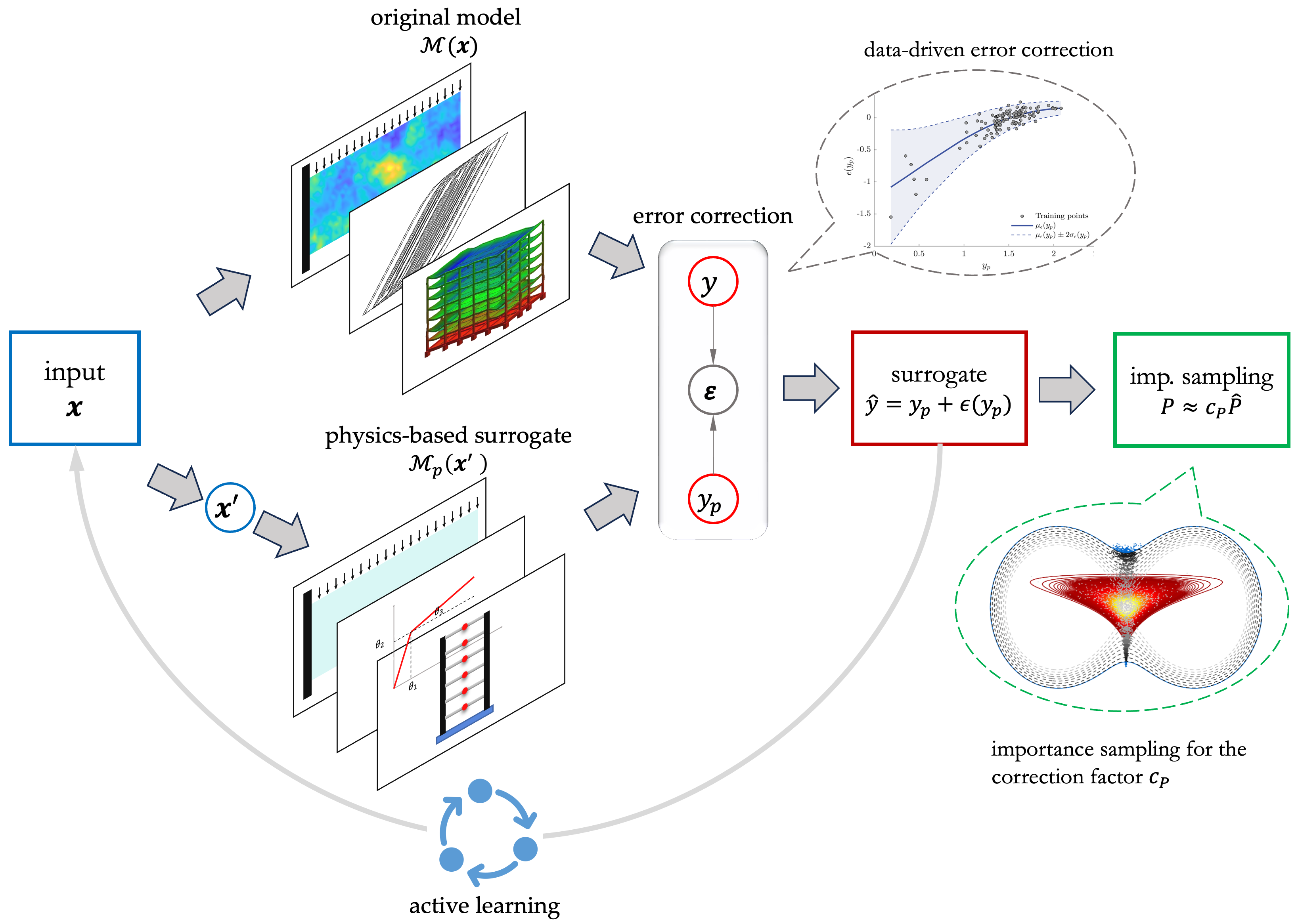
Figure 1: Schematic of the proposed surrogate modeling method for rare event simulation. The physics-based surrogate model $y_{p}=\mathcal{M}_{p}(\boldsymbol{x}^{\prime};\boldsymbol{\theta}_{p})$ contains tunable control parameters $\boldsymbol{\theta}_{p}$ to be optimized in the training process. The error correction function $\epsilon(y_{p})$ is modeled in the space of $y_{p}$ by heteroscedastic Gaussian process to account for input-dependent noises. The active learning adaptively enriches the training set with a learning criterion to highlight contributions from the rare event region. The importance sampling estimates the correction factor $c_{P}$ to improve the probability estimation of the surrogate model.

3 Training of the coupled physics-data-driven surrogate model

3.1 Optimization of parametric physical models

In physics-based surrogate modeling, the response predictions of the surrogate model can be inaccurate but still be mildly/highly correlated with that of the original model. The statistical correlation between the surrogate and original model responses has a decisive impact on the noise of the error correction term (see Figure 2 for a simple illustration)–higher correlation indicates smaller noise. Pearson, Spearman’s Rank, and Kendall’s Tau correlation coefficients are popular indices for quantifying the correlation between two random variables [62]. The Pearson correlation coefficient can only reflect the linear correlation, while the Spearman’s Rank and Kendall’s Tau correlation coefficients can handle the nonlinear dependency. In our context, the physics-based surrogate model by construction is a simplification of the original model. Thus, a mildly nonlinear correlation is expected. Consequently, the Pearson correlation coefficient is sufficient. The Spearman’s Rank and Kendall’s Tau correlation coefficients can be readily implemented into the proposed surrogate modeling method, but we did not observe an improvement in performance for the numerical examples we have studied. It is worth mentioning that mutual information [63, 64] is a more general metric for measuring dependency between two random variables, but the sample estimate of mutual information involves additional assumptions on the joint distributions.

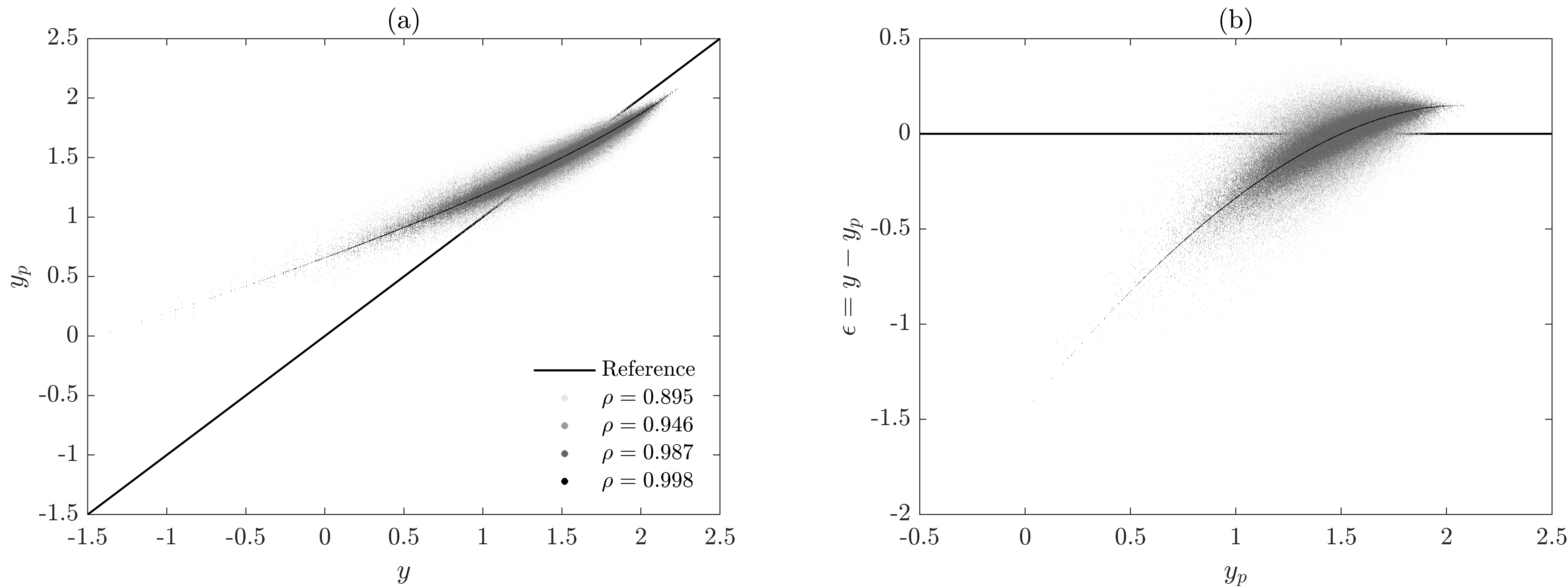
Figure 2: Impact of the correlation between surrogate and original model responses on the noise of the error correction function. For illustration, $Y$ and $Y_{p}$ are assumed to be lognormal with a Pearson correlation coefficient varying among $\rho=0.895$, $0.946$, $0.987$, and $0.998$. It is seen that the noise in the error $\epsilon=y-y_{p}$ decreases with the increase of the correlation coefficient. It is also clear that an exact interpolation model should be avoided when $\epsilon$ is noisy.

Because rare event probabilities are dominated by conditional distributions, the correlation between $Y$ and $Y_{p}$ generated by $\boldsymbol{X}\sim f_{\boldsymbol{X}}(\boldsymbol{x})$ may not be an ideal objective for optimizing the surrogate model. A remedy is to consider the correlation between $\mathbb{I}_{\leq 0}\left(Y\right)$ and $\mathbb{I}_{\leq 0}\left(Y_{p}\right)$, where $\mathbb{I}_{\leq 0}:\mathbb{R}\mapsto\{0,1\}$ is a binary indicator function for the rare event. The computational issue of this approach is that the samples generated from $f_{\boldsymbol{X}}(\boldsymbol{x})$ are unlikely to fall into the rare event and thus the estimation of the Pearson correlation coefficient between $\mathbb{I}_{\leq 0}\left(Y\right)$ and $\mathbb{I}_{\leq 0}\left(Y_{p}\right)$ would be inaccurate. In this work, we adopt active learning to adaptively enrich the training set $\mathcal{D}=\{(\boldsymbol{x}^{i},\mathcal{M}(\boldsymbol{x}^{(i)}))\}$ toward the critical region around $\{\mathcal{M}(\boldsymbol{x})=0\}$. Using the training set $\mathcal{D}$, the sample correlation coefficient emphasizes the contribution from the rare event. This is essentially equivalent to redefining the correlation between $\mathcal{M}(\boldsymbol{X})$ and $(\mathcal{M}_{p}\circ\psi)(\boldsymbol{X})$ using an active learning-controlled importance sampling distribution rather than the original $f_{\boldsymbol{X}}(\boldsymbol{x})$. To summarize, the optimization for the physics-based surrogate model $(\mathcal{M}_{p}\circ\psi)(\boldsymbol{x};\boldsymbol{\theta}_{p})$ is formulated as

$$\boldsymbol{\theta}^{\ast}_{p} =\mathop{\arg\max}\limits_{\boldsymbol{\theta}_{p}}\rho_{YY_{p}}(\boldsymbol{\theta}_{p}|\mathcal{D})$$ (3)

$$=\mathop{\arg\max}\limits_{\boldsymbol{\theta}_{p}}\frac{\left\langle(\mathcal{M}(\boldsymbol{X})-\langle\mathcal{M}(\boldsymbol{X})\rangle_{\mathcal{D}})\left((\mathcal{M}_{p}\circ\psi)(\boldsymbol{X};\boldsymbol{\theta}_{p})-\langle(\mathcal{M}_{p}\circ\psi)(\boldsymbol{X};\boldsymbol{\theta}_{p})\rangle_{\mathcal{D}}\right)\right\rangle_{\mathcal{D}}}{\sqrt{\left\langle(\mathcal{M}(\boldsymbol{X})-\langle\mathcal{M}(\boldsymbol{X})\rangle_{\mathcal{D}})^{2}\right\rangle_{\mathcal{D}}\left\langle((\mathcal{M}_{p}\circ\psi)(\boldsymbol{X};\boldsymbol{\theta}_{p})-\left\langle(\mathcal{M}_{p}\circ\psi)(\boldsymbol{X};\boldsymbol{\theta}_{p})\right\rangle_{\mathcal{D}})^{2}\right\rangle_{\mathcal{D}}}}\,,$$

where $\langle\cdot\rangle$ denotes sample mean.

Before solving Eq. (3), we need to design $\boldsymbol{\theta}_{p}$ for the physics-based surrogate model, i.e., determine which parameters are tunable. For specific applications, engineering judgement can be used to design $\boldsymbol{\theta}_{p}$. A more objective approach is to adopt a parsimonious principle to select a minimum number of parameters that can achieve a relatively high $\max_{\boldsymbol{\theta}_{p}}\rho_{YY_{p}}(\boldsymbol{\theta}_{p}|\mathcal{D})$. This principle can be materialized as an incremental approach to start with a single tunable parameter and iteratively augment if $\max_{\boldsymbol{\theta}_{p}}\rho_{YY_{p}}(\boldsymbol{\theta}_{p}|\mathcal{D})$ can be significantly improved. In the simulation test cases of civil and mechanical systems, we have investigated the use of elastic modulus, damping ratio, stiffness, and yield displacement as tunable parameters, where $\max_{\boldsymbol{\theta}_{p}}\rho_{YY_{p}}(\boldsymbol{\theta}_{p}|\mathcal{D})$ can typically achieve $0.95$.

Finally, the optimization in Eq. (3) can be solved by gradient-free metaheuristic algorithms [65]. Provided with a training set $\mathcal{D}$, solving Eq. (3) does not involve additional simulations of the original model, but it requires simulations of the physics-based surrogate model. If $\mathcal{D}$ is enriched by active learning, Eq. (3) needs to be re-solved; the solution from the previous training set can be used as a warm initial guess.

3.2 Error corrections using heteroscedastic Gaussian process

Given a training set $\mathcal{D}=\{(\boldsymbol{x}^{i},\mathcal{M}(\boldsymbol{x}^{(i)}))\}$ and the solution of Eq. (3), we obtain the training set for the error correction, $\mathcal{D}_{\epsilon}=\{(y_{p}^{(i)},\varepsilon^{(i)})\}$, where $y_{p}^{(i)}=(\mathcal{M}_{p}\circ\psi)(\boldsymbol{x}^{(i)};\boldsymbol{\theta}_{p}^{*})$ and $\varepsilon^{(i)}=\mathcal{M}(\boldsymbol{x}^{(i)})-(\mathcal{M}_{p}\circ\psi)(\boldsymbol{x}^{(i)};\boldsymbol{\theta}_{p}^{*})$. Using $\mathcal{D}_{\epsilon}$, we train a heteroscedastic Gaussian process [59, 60, 61] to model $\epsilon(y_{p})$, expressed by

$${\epsilon}(y_{p};\boldsymbol{\theta}_{\epsilon})=f(y_{p};\boldsymbol{\theta}_{f})+\tau(y_{p};\boldsymbol{\theta}_{\tau})\,,$$ (4)

where $\boldsymbol{\theta}_{\epsilon}=\boldsymbol{\theta}_{f}\cup\boldsymbol{\theta}_{\tau}$, $f(y_{p})\sim\mathcal{GP}(\mu_{f}(y_{p}),k_{f}(y_{p},y_{p}^{\prime});\boldsymbol{\theta}_{f})$ is a Gaussian process with hyperparameters $\boldsymbol{\theta}_{f}$ to model the mean $\mu_{f}(y_{p})$ and kernel $k_{f}(y_{p},y_{p}^{\prime})$, $\tau(y_{p})\sim\mathcal{N}(0,\exp(g(y_{p})))$ is an input-dependent Gaussian noise with zero mean and variance $\exp(g(y_{p}))$, and $g(y_{p})\sim\mathcal{GP}(\mu_{g},k_{g}(y_{p},y_{p}^{\prime});\boldsymbol{\theta}_{g})$ is another Gaussian process with hyperparameters $\boldsymbol{\theta}_{g}$ to model the mean $\mu_{g}$ and kernel $k_{g}(y_{p},y_{p}^{\prime})$.

The introduction of the heteroscedastic Gaussian noise is essential in this study because the mapping from $y_{p}$ to $y$ can be one-to-many. The use of heteroscedastic Gaussian process comes with a price of increasing the number of hyperparameters for the Gaussian process model, and the analytical marginal likelihood and prediction equations for the homoscedastic Gaussian process are no longer useful [59, 60, 61]. The hyperparameters $\boldsymbol{\theta}_{f}$ and $\boldsymbol{\theta}_{g}$ can be approximated by maximizing the following lower bound of the exact marginal likelihood [59]:

$$F(\boldsymbol{\mu},\boldsymbol{\Sigma})=\textrm{log}f_{\mathcal{N}}(\boldsymbol{\varepsilon};\boldsymbol{0},\boldsymbol{K}_{f}+\boldsymbol{R})-\frac{1}{4}\textrm{tr}(\boldsymbol{\Sigma})-\textrm{KL}(f_{\mathcal{N}}(\boldsymbol{g};\boldsymbol{\mu},\boldsymbol{\Sigma})||f_{\mathcal{N}}(\boldsymbol{g};\mu_{g}\boldsymbol{1},\boldsymbol{K}_{g}))\,,$$ (5)

where $\boldsymbol{\mu}$ and $\boldsymbol{\Sigma}$ are the variational mean vector and covariance matrix to be determined alongside with the hyperparameters $\boldsymbol{\theta}_{f}$ and $\boldsymbol{\theta}_{g}$, $\boldsymbol{\varepsilon}=[{\varepsilon}^{(1)},{\varepsilon}^{(2)},...]^{\intercal}$ are from the training set $\mathcal{D}_{\epsilon}$, $\boldsymbol{0}$ and $\boldsymbol{1}$ are vectors of zeros and ones, $\boldsymbol{K}_{f}$ and $\boldsymbol{K}_{g}$ are respectively the covariance matrices of the Gaussian processes $f(y_{p})$ and $g(y_{p})$, $\boldsymbol{R}$ is a diagonal matrix with entries $R_{i,i}=\exp(\mu_{i}-\Sigma_{i,i}/2)$, $i=1,2,...$, $f_{\mathcal{N}}$ denotes the probability density function of a multivariate Gaussian distribution, tr denotes matrix trace, and $\textrm{KL}(\cdot||\cdot)$ denotes the Kullback–Leibler divergence between two probability density functions.

Once the hyperparameters $\boldsymbol{\theta}_{f}$ and $\boldsymbol{\theta}_{g}$ are estimated, the predictions for the mean and variance of $\epsilon(y_{p}^{\ast})$ at $y_{p}^{\ast}$ are obtained from [59]

$$\mu_{{\epsilon}}(y^{\ast}_{p})=\boldsymbol{k}_{f\ast}^{\intercal}(\boldsymbol{K}_{f}+\boldsymbol{R})^{-1}\boldsymbol{\varepsilon}\,,$$ (6)

and

$$\sigma_{{\epsilon}}^{2}(y_{p}^{\ast})=\exp\left(\boldsymbol{k}_{g\ast}^{\intercal}(\boldsymbol{\Lambda}-\tfrac{1}{2}\boldsymbol{I})\boldsymbol{1}+\mu_{g}+\frac{k_{g\ast\ast}-\boldsymbol{k}_{g\ast}^{\intercal}(\boldsymbol{K}_{g}+\boldsymbol{\Lambda}^{-1})^{-1}\boldsymbol{k}_{g\ast}}{2}\right)+k_{f\ast\ast}-\boldsymbol{k}_{f\ast}^{\intercal}(\boldsymbol{K}_{f}+\boldsymbol{R})^{-1}\boldsymbol{k}_{f\ast}\,,$$ (7)

respectively, where $k_{f\ast\ast}=k_{f}(y_{p}^{\ast},y_{p}^{\ast})$, $k_{g\ast\ast}=k_{g}(y_{p}^{\ast},y_{p}^{\ast})$, $\boldsymbol{k}_{f\ast}=[k_{f}(y_{p}^{(1)},y_{p}^{\ast}),k_{f}(y_{p}^{(2)},y_{p}^{\ast}),...]^{\intercal}$ and $\boldsymbol{k}_{g\ast}=[k_{g}(y_{p}^{(1)},y_{p}^{\ast}),k_{g}(y_{p}^{(2)},y_{p}^{\ast}),...]{{}^{\intercal}}$, $\boldsymbol{I}$ is the identity matrix, and $\boldsymbol{\Lambda}$ is a positive semi-definite diagonal matrix introduced to re-parameterize $\boldsymbol{\mu}$ and $\boldsymbol{\Sigma}$ in a reduced order.

The mean $\mu_{{\epsilon}}(y^{\ast}_{p})$ can be used as the prediction of the surrogate modeling error at $y_{p}^{\ast}$, and $\sigma_{{\epsilon}}^{2}(y_{p}^{\ast})$ quantifies the uncertainty of this prediction. The later quantity is desirable in active learning. It is worth noting that the roles of the heteroscedastic Gaussian process involve quantifying the noise and correcting the (mean) predictions of the physics-based surrogate model (see Figure 3); it cannot reduce the noise.

Figure 3: Heteroscedastic Gaussian process for error correction. Following Figure 2, for $\rho=0.946$, a heteroscedastic Gaussian process is trained to fit the error. It is seen that the heteroscedastic errors are well-captured. The heteroscedastic Gaussian process corrects the surrogate model predictions, however, the improvement on correlation coefficient is marginal: $0.949$ for $y$ and $y_{p}+\mu_{{\epsilon}}(y_{p})$ compared with the original $\rho=0.946$.

3.3 Adaptive training by active learning

Given an initial training set $\mathcal{D}=\{(\boldsymbol{x}^{(i)},\mathcal{M}(\boldsymbol{x}^{(i)}))\}_{i=1}^{N_{0}}\equiv\mathcal{D}_{\boldsymbol{x}}\times\mathcal{D}_{y}$, we sequentially train the physics-based surrogate model $y_{p}=(\mathcal{M}_{p}\circ\psi)(\boldsymbol{x};\boldsymbol{\theta}_{p})$ and the error correction function $\epsilon(y_{p};\boldsymbol{\theta}_{\epsilon})$ to obtain the initial surrogate model $\hat{y}=(\mathcal{M}_{p}\circ\psi)(\boldsymbol{x};\boldsymbol{\theta}_{p})+\epsilon(y_{p};\boldsymbol{\theta}_{\epsilon})$. Subsequently, we initiate an active learning process to iteratively enrich the training set $\mathcal{D}$ and update the surrogate model. Hereafter, we develop an active learning process tailored to the physics-data-driven surrogate modeling.

Provided with the current surrogate model, we first define a critical learning region $\Omega_{c}$ as:

$$\Omega_{c}=\left\{\boldsymbol{x}\in\mathbb{R}^{n}:\frac{\left|y_{p}+\mu_{{\epsilon}}(y_{p})\right|}{\sigma_{{\epsilon}}(y_{p})}\leqslant\delta,\,\,\,y_{p}=(\mathcal{M}_{p}\circ\psi)(\boldsymbol{x};\boldsymbol{\theta}_{p})\right\}\,,$$ (8)

where $\delta>0$ is a cutoff value for the learning region, and $\mu_{\epsilon}(y_{p})$ and $\sigma_{\epsilon}(y_{p})$ are respectively the mean and standard deviation of the Gaussian process error correction at $y_{p}$.

Next, we generate a candidate training set ${\mathcal{X}}_{c}=\{\boldsymbol{x}^{(i)}\}_{i=1}^{N}$ through

$$\boldsymbol{X}^{(i)}\sim\mathbb{I}_{\Omega_{c}}\left(\boldsymbol{x}\right)f_{\boldsymbol{X}}(\boldsymbol{x})\,,$$ (9)

where $\mathbb{I}_{\Omega_{c}}:\mathbb{R}^{n}\mapsto\{0,1\}$ is an indicator function for $\{\boldsymbol{x}\in\Omega_{c}\}$ and the normalizing constant for the density $\mathbb{I}_{\Omega_{c}}\left(\boldsymbol{x}\right)f_{\boldsymbol{X}}(\boldsymbol{x})$ is omitted for simplicity. To reduce surrogate model simulations and improve the scalability toward low probability estimations, the sequential Monte Carlo [17, 18, 19] is used to generate ${\mathcal{X}}_{c}$.

Given ${\mathcal{X}}_{c}$, the next training point $\boldsymbol{x}^{\ast}$ is identified by:

$$\boldsymbol{x}^{\ast}=\mathop{\arg\max}\limits_{\boldsymbol{x}\in{\mathcal{X}}_{c}}\left(\mathop{\min}\limits_{y_{p}^{\prime}\in{\mathcal{Y}_{p}}}\left\|{y}_{p}-{y}_{p}^{\prime}\right\|\right),\,\,\,y_{p}=(\mathcal{M}_{p}\circ\psi)(\boldsymbol{x};\boldsymbol{\theta}_{p})\,,$$ (10)

where $\mathcal{Y}_{p}=\{y_{p}=(\mathcal{M}_{p}\circ\psi)(\boldsymbol{x};\boldsymbol{\theta}_{p}):\boldsymbol{x}\in\mathcal{D}_{\boldsymbol{x}}\}$ is a set of $y_{p}$ predictions from existing training samples. This equation picks the point in $\mathcal{X}_{c}$ that differs (in terms of $y_{p}$) the most from the existing training points, aiming to achieve sparsely distributed training points in the space of $y_{p}$. This learning criterion is a relaxation of the classic U-function-based learning [30] through introducing additional, seemingly redundant, distance-based selection to enforce sparsity. This relaxation is necessary because the prediction uncertainty term $\sigma_{\epsilon}(y_{p})$ of the U-function, which influences the “sparsity” of the U-function-based training point selection, is not only affected by the distance to existing training points, but also contributed, sometimes dominantly, by the inherent noise of the surrogate model. In the conventional application [30, 31, 32] of active learning-based Gaussian process modeling, the training data does not have inherent stochastic noise, and the distance-based selection in Eq. (10) can be unnecessary. Incidentally, the constructions of Eq. (8) and Eq. (9) are still meaningful even for noise-free scenarios, because they facilitate the use of efficient sampling methods to identify the low-probability critical region to propose training points.

Provided with the next training point $\boldsymbol{x}^{\ast}$, the original model is simulated to obtain $y^{\ast}=\mathcal{M}(\boldsymbol{x}^{\ast})$, the training set $\mathcal{D}$ is augmented to include $(\boldsymbol{x}^{\ast},y^{\ast})$, and the surrogate model is updated. The learning process is repeated until a stopping criterion is reached. The simple stopping criterion adopted in this work is expressed by $\frac{\left|\hat{P}^{(m+1)}-\hat{P}^{(m)}\right|}{\hat{P}^{(m+1)}}\leqslant\eta$, $m=0,1,...$, i.e., the learning stops if the rare event probability estimation is stable. An alternative stopping criterion is to check the prediction uncertainty of the rare event probability [66, 67]; this approach typically requires more learning steps to stop but favors accuracy.

The implementation details for the training of the coupled physics-data-driven surrogate model are presented in Appendix 16. Due to the presence of inherent noises in the surrogate model (recall Figure 3(b)), the probability estimation has no guarantee of convergence to the correct probability. To address this issue, a final importance sampling step will be introduced in the following section.

4 Importance sampling using the coupled physics-data-driven surrogate model

The target rare event probability can be formulated as

$$P=\int_{\boldsymbol{x}\in\mathbb{R}^{n}}\mathbb{I}_{\leq 0}\left(\mathcal{M}(\boldsymbol{x})\right)f_{\boldsymbol{X}}(\boldsymbol{x})\mathrm{d}\boldsymbol{x}\,.$$ (11)

The importance sampling rewrites the integral in Eq. (11) by introducing an importance density $h(\boldsymbol{x})$, i.e.,

$$P=\int_{\boldsymbol{x}\in\mathbb{R}^{n}}\mathbb{I}_{\leq 0}\left(\mathcal{M}(\boldsymbol{x})\right)\frac{f_{\boldsymbol{X}}(\boldsymbol{x})}{h(\boldsymbol{x})}h(\boldsymbol{x})\mathrm{d}\boldsymbol{x}\,.$$ (12)

The support of the importance density $h(\boldsymbol{x})$ should cover the rare event, and the optimal importance density is [10]

$$h^{\ast}(\boldsymbol{x})=\frac{\mathbb{I}_{\leq 0}\left(\mathcal{M}(\boldsymbol{x})\right)f_{\boldsymbol{X}}(\boldsymbol{x})}{P}\,.$$ (13)

Due to the high correlation between the original and surrogate model responses, it is tempting to use the following importance density from the surrogate model as an approximation for the optimal density.

$$\hat{h}(\boldsymbol{x})=\frac{\mathbb{I}_{\leq 0}\left((\mathcal{M}_{p}\circ\psi)(\boldsymbol{x};\boldsymbol{\theta}_{p})+\mu_{{\epsilon}}((\mathcal{M}_{p}\circ\psi)(\boldsymbol{x};\boldsymbol{\theta}_{p});\boldsymbol{\theta}_{\epsilon})\right)f_{\boldsymbol{X}}(\boldsymbol{x})}{\hat{P}}\,,$$ (14)

where $\hat{P}$ is the rare event probability estimated from the surrogate model. However, there is no guarantee that the target rare event is an improper subset of the support of $\hat{h}(\boldsymbol{x})$. Therefore, $\hat{h}(\boldsymbol{x})$ cannot be directly employed as an importance density. One remedy is to replace the binary indicator function in Eq. (14) by a smooth approximation [17, 56], so that $\hat{h}(\boldsymbol{x})$ becomes nonzero everywhere. This approach requires the tuning of a relaxation parameter associated with the smooth approximation of the indicator function.

An alternative remedy, which is adopted in this paper, is to use the following identity derived from properties of conditional probability [56]:

$$P=c_{P}\cdot\hat{P}\equiv\frac{\int_{\boldsymbol{x}\in\mathbb{R}^{n}}\mathbb{I}_{\leq 0}\left(\mathcal{M}(\boldsymbol{x})\right)\hat{h}(\boldsymbol{x})\mathrm{d}\boldsymbol{x}}{\int_{\boldsymbol{x}\in\mathbb{R}^{n}}\mathbb{I}_{\leq 0}\left((\mathcal{M}_{p}\circ\psi)(\boldsymbol{x};\boldsymbol{\theta}_{p})+\mu_{{\epsilon}}((\mathcal{M}_{p}\circ\psi)(\boldsymbol{x};\boldsymbol{\theta}_{p});\boldsymbol{\theta}_{\epsilon})\right)h^{\ast}(\boldsymbol{x})\mathrm{d}\boldsymbol{x}}\,\hat{P}\,,$$ (15)

where $c_{P}$ is the correction factor for the surrogate model-based rare event probability estimation. The numerator represents the conditional probability that the original rare event given the surrogate rare event, while the denominator represents the conditional probability that the surrogate rare event given the original rare event. Ideally, the correction factor $c_{P}$ should be close to $1$; therefore, $c_{P}$ can be used as a performance measure of the surrogate model. The conditional probabilities in Eq. (15) can be estimated by Monte Carlo simulation with Markov Chain Monte Carlo algorithms [68, 69] to generate samples from $h^{*}(\boldsymbol{x})$ and $\hat{h}(\boldsymbol{x})$. For a well-trained surrogate model, the overlap between $h^{*}(\boldsymbol{x})$ and $\hat{h}(\boldsymbol{x})$ is expected to be significant; consequently, the computational cost to estimate $c_{P}$ would be small. However, theoretically speaking, Eq. (15) implies that the surrogate model solution $\hat{P}$ can be highly accurate even when the surrogate rare event does not largely overlap with the actual rare event; this is illustrated by Figure 4. Finally, the implementation details of the importance sampling using Eq. (15) are presented in Appendix 17.

Figure 4: Importance sampling for the coupled physics-data-driven surrogate model. The true rare event from the original model is $E_{1}\cup E_{3}$, and the “surrogate” rare event from the surrogate model is $E_{2}\cup E_{3}$. Eq. (15) is derived from the identity $\mathbb{P}\left(E_{1}\cup E_{3}\right)=\mathbb{P}\left(E_{2}\cup E_{3}\right)\frac{\mathbb{P}\left(E_{3}\right)/{\mathbb{P}\left(E_{2}\cup E_{3}\right)}}{\mathbb{P}\left(E_{3}\right)/{\mathbb{P}\left(E_{1}\cup E_{3}\right)}}$. It follows that if $\mathbb{P}\left(E_{1}\right)=\mathbb{P}\left(E_{2}\right)$, $P=\hat{P}$, i.e., $\hat{P}$ can be accurate even when the overlap $E_{3}$ is not significant. This condition can be met if $\hat{Y}$ is an unbiased estimator of $Y$ for the region $E_{1}\cup E_{2}\cup E_{3}$, supporting the proposed approach of training a Gaussian process to correct the bias in the critical region identified by active learning.

5 Numerical examples

In this section, we will investigate (1) a static problem of a linear elastic cantilever beam with material properties modeled by a Gaussian random field, (2) a dynamic problem of a nonlinear viscous damper under white noise excitation, and (3) a dynamic problem of a multi-degree-of-freedom hysteretic system under white noise excitation. Three schemes are investigated to construct physics-based surrogate models. Specifically, homogenization of material properties is considered in the first example, statistical linearization is used in the second example, and relaxation of the numerical solver is adopted in the third example.

5.1 Example 1: A linear elastic cantilever beam

Consider a linear elastic cantilever beam of length $5$m and width $2$m subjected to 20 evenly spaced concentrated loads on the upper edge with the magnitudes of $Q=500\mathrm{kN}$, shown in Figure 5. The Poisson ratio of the beam is $\nu=0.3$. The reference/original computational model is represented by a discretization of the beam into $50\times 20=1000$ four-node quadrilateral elements, and the elastic modulus of the beam is characterized by a homogeneous random field $E(x,y)$ with a discretization of $1000$ Gaussian random variables compatible with the spatial discretization. The autocorrelation function of the Gaussian random field is modeled by the isotropic exponential model $R_{E}(\Delta_{x},\Delta_{y})=\exp\left(-\sqrt{\Delta_{x}^{2}+\Delta_{y}^{2}}/l\right)$ with the correlation length $l=10\mathrm{m}$. The mean value and standard deviation of the marginal Gaussian distribution are $\mu_{E}=200\mathrm{GPa}$ and $\sigma_{E}=30\mathrm{GPa}$, respectively. The physics-based surrogate model is constructed via a simple homogenization of the random field of the elastic modulus:

$$E_{p}=a_{E}\bar{E}+b_{E}\,,$$ (16)

where $\{a_{E},b_{E}\}=\boldsymbol{\theta}_{p}$ are tunable parameters of the physics-based surrogate model, and $\bar{E}$ represents the average of the $1000$ Gaussian random variables. The initial values of $a_{E}$ and $b_{E}$ are set to be $1$ and $0$, respectively. The rare event of interest is defined as the vertical displacement of point A exceeds a prescribed threshold of $0.0032\mathrm{m}$, expressed by

$$\{y=0.0032-d_{A}\leq 0\}\,,$$ (17)

where $d_{A}$ is the vertical displacement of point A.

Figure 5: Physics-based surrogate model of a linear elastic cantilever beam. (a) original model: the spatial domain of the beam is discretized into $50\times 20=1000$ four-node quadrilateral elements. The elastic modulus of the beam is characterized by a homogeneous random field $E(x,y)$ with a discretization of $1000$ Gaussian random variables compatible with the spatial discretization; (b) physics-based surrogate model: the whole beam is represented by a single four-node quadrilateral element. The elastic modulus is assumed to be a homogenization of the random field, i.e., $E_{p}=a_{E}\bar{E}+b_{E}$, where $a_{E}$ and $b_{E}$ are tunable parameters, and $\bar{E}$ is the average of the $1000$ Gaussian random variables.

The coupled physics-data-driven surrogate model is trained with $100$ random initial training points in conjunction with $57$ training points identified by active learning, leading to a total of $157$ runs of the original model. The heteroscedastic Gaussian process model for the error correction at the final learning stage is shown in Figure 6. It is seen that the heteroscedastic Gaussian process can model the noisy errors. The optimization histories of the correlation coefficient ${\rho}$, the parameter $b_{E}$, and the probability $\hat{P}$ are shown in Figure 7, and their final values are $0.9861$, $20.5$GPa, and $2.1110\times 10^{-5}$, respectively. Notice that the correlation coefficient value of $0.9861$ is estimated using the training data, the “global” correlation coefficient is around $0.9605$. The reference rare event probability obtained by the subset simulation with $4.6\times 10^{4}$ samples is $3.6130\times 10^{-5}$. The scatter plots of $y_{p}$ and $y_{p}+\epsilon(y_{p})$ against $y$ are shown in Figure 8. It is seen that the response predictions of the physics-based surrogate model are highly correlated with the responses of the original model, and the data-driven error correction can improve the bias of the surrogate predictions. Finally, the importance sampling is implemented to further improve the probability estimation. To achieve a coefficient of variation of $5\%$, 800 runs of the original model are required and the final estimate of probability is $3.4326\times 10^{-5}$. This indicates that the correction factor $c_{P}$ (recall Eq. (12)) for the surrogate model solution is $1.63$.

Figure 6: Heteroscedastic Gaussian process model of the error correction at the final learning stage for Example 1. The Gaussian process model is obtained from $100(\text{initial})+57(\text{active learning})$ training data. It is seen that the heteroscedastic Gaussian process model can capture the noisy errors.

Figure 7: Optimization histories of the proposed method for Example 1. (a) the correlation coefficient ${\rho}$ between $Y_{p}$ and $Y$ at the training points achieves $0.9861$; (b) the tunable parameter $b_{E}$ for the physics-based surrogate model converges to $20.5\mathrm{GPa}$; (c) the probability estimation $\hat{P}$ converges to $2.1110\times 10^{-5}$. The reference solution from subset simulation with $4.6\times 10^{4}$ samples is $3.6130\times 10^{-5}$.

Figure 8: Response predictions of the physics-based surrogate model and the coupled physics-data-driven surrogate model for Example 1. The response prediction of the physics-based surrogate model $Y_{p}$ is highly correlated with the true responses $Y$, and the data-driven error correction improves the bias. The estimated correlation coefficient between $Y$ and $Y_{p}$ as well as that between $Y$ and $Y_{p}+\mu_{\epsilon}(Y_{p})$ are both around $0.9605$. This is expected because from Figure 6 we can observe that the error correction $\epsilon$ is linear with respect to $y_{p}$.

5.2 Example 2: An oscillator with nonlinear viscous damper

Consider an oscillator with nonlinear viscous damper under a Gaussian white noise excitation with the equation of motion expressed as

$$m\ddot{u}(t)+c\dot{u}(t)+ku(t)+c_{d}\mathrm{sign}(\dot{u}(t))\left|\dot{u}(t)\right|^{\alpha_{d}}=-m\ddot{u}_{g}(t)\,,$$ (18)

where $m=3000\mathrm{kg}$, $c=3000\mathrm{N/(m/s)}$, and $k=3\times 10^{5}\mathrm{N/m}$ are the mass, damping, and stiffness of the oscillator, respectively, $u(t)$, $\dot{u}(t)$, and $\ddot{u}(t)$ are the displacement, velocity, and acceleration of the oscillator, respectively, $c_{d}=800\mathrm{N/(m/s)}^{\alpha_{d}}$ and $\alpha_{d}=0.3$ are the damping coefficient and velocity exponent of the nonlinear viscous damper, respectively, $\mathrm{sign}(\cdot)$ is the sign function, and $\ddot{u}_{g}(t)$ is the acceleration excitation.

The excitation has a duration of $15$ seconds. Using the spectral representation method [70], the white noise can be discretized into a finite set of Gaussian variables:

$$\ddot{u}_{g}(\boldsymbol{X},t)=\sum_{i=1}^{D/2}\sqrt{2S_{0}\Delta\omega}\left(X_{i}\textrm{cos}(\omega_{i}t)+\bar{X}_{i}\mathrm{sin}(\omega_{i}t)\right)\,,$$ (19)

where $X_{i}$ and $\bar{X}_{i}$, $i=1,2,...,D/2$, are mutually independent standard normal variables, $D=1000$, $\Delta\omega=2\omega_{\max}/D$ is the frequency increment with $\omega_{\max}=25\pi$ being the upper cutoff angular frequency, $\omega_{i}=(i-0.5)\Delta\omega$ is the discretized frequency points, and $S_{0}=5\times 10^{-3}\mathrm{m^{2}/s^{3}}$ is the intensity of the white noise.

To obtain the physics-based surrogate model, the nonlinear equation of motion shown in Eq. (18) is linearized into

$$m\ddot{u}(t)+(c+c_{e})\dot{u}(t)+ku(t)=-m\ddot{u}_{g}(t)\,,$$ (20)

where $\{c_{e}\}=\boldsymbol{\theta}_{p}$ is the equivalent damping coefficient used as the tuning parameter of the physics-based surrogate model. The rare event of interest is defined as the peak absolute displacement of the oscillator exceeding a threshold of $0.06$m, expressed by

$$\left\{y=0.06-\sup_{t\in[0,15]}|u(t)|\leq 0\right\}\,.$$ (21)

The initial value of $c_{e}$ for optimization is determined by the traditional statistical linearization method [71].

The coupled physics-data-driven surrogate model is trained using $100(\text{initial})+86(\text{active learning})$ samples, and the heteroscedastic Gaussian process model for error correction at the final learning stage is shown in Figure 9. The optimization histories of the correlation coefficient ${\rho}$, the equivalent damping coefficient $c_{e}$, and the probability $\hat{P}$ are shown in Figure 10; their final values are $0.9980$, $1973.3$N/(m/s), and $2.5310\times 10^{-7}$, respectively. The probability predicted by the coupled surrogate model is $2.5310\times 10^{-7}$, which is close to the reference solution $2.9540\times 10^{-7}$ obtained from subset simulation using $6.49\times 10^{4}$ samples. The scatter plots of $y_{p}$ and $y_{p}+\epsilon(y_{p})$ against $y$ are shown in Figure 11. The correction factor $c_{P}$ in the importance sampling step is estimated to be $1.25$ using an additional $800$ runs of the original model, leading to a final probability estimate of $3.1536\times 10^{-7}$.

Figure 9: Heteroscedastic Gaussian process model of the error correction at the final learning stage for Example 2. The surrogate model is trained using $100(\text{initial})+86(\text{active learning})$ samples. The heteroscedastic Gaussian process model captures the noisy errors.

Figure 10: Optimization histories of the proposed method for Example 2. (a) the correlation coefficient ${\rho}$ between $Y_{p}$ and $Y$ at the training points achieves $0.9980$; (b) the equivalent damping parameter $c_{e}$ for the physics-based surrogate model stops at $1973.3\mathrm{N/(m/s)}$; (c) the probability estimation $\hat{P}$ converges to $2.5310\times 10^{-7}$. The reference solution of subset simulation with $6.49\times 10^{4}$ samples is $2.9540\times 10^{-7}$.

Figure 11: Response predictions of physics-based surrogate model and coupled physics-data-driven surrogate model for Example 2. The response prediction of the physics-based surrogate model $Y_{p}$ is highly correlated with the true responses $Y$, and the data-driven error correction improves the bias. The estimated correlation coefficients between $Y$ and $Y_{p}$ and that between $Y$ and $Y_{p}+\mu_{\epsilon}(Y_{p})$ are $0.9783$ and $0.9791$, respectively. This tiny difference originates from the weak nonlinearity in Figure 9.

5.3 Example 3: A multi-degree-of-freedom hysteretic system

Consider a 6-degree-of-freedom shear-type hysteretic system under ground motion excitation, shown in Figure 12. The mass and initial stiffness of each storey are $m_{i}=8000\mathrm{kg}$ and $k_{i}=1\times 10^{7}\mathrm{N/m}$, $i=1,2,...,6$, respectively. Rayleigh damping is assumed for the hysteretic system with a damping ratio of $5\%$ for the 1st and 6th mode of the system. The restoring force of each storey is described by the Bouc-Wen model [72] as follows:

$$f_{i}(t)=\alpha_{i}k_{i}u_{i}(t)+(1-\alpha_{i})k_{i}z_{i}(t)\,,$$ (22)

$$\dot{z_{i}}(t)=g_{i}(\dot{u_{i}}(t),z_{i}(t))=\phi_{i}\dot{u_{i}}(t)-\varphi_{i}\left|\dot{u_{i}}(t)\right|z_{i}(t)\left|z_{i}(t)\right|^{\gamma_{i}-1}-\psi_{i}\dot{u_{i}}(t)\left|z_{i}(t)\right|^{\gamma_{i}}\,,$$ (23)

where $\alpha_{i}=0.1$ is the stiffness reduction ratio of the $i$-th storey; $u_{i}(t)$, $\dot{u_{i}}(t)$, and $z_{i}(t)$ are the relative displacement, relative velocity, and the hysteretic displacement of the $i$-th storey, respectively; $\phi_{i}=1$, $\varphi_{i}=\psi_{i}=1/(2x_{yi}^{\gamma_{i}})$, and $\gamma_{i}=1$ are the shape parameters of the hysteresis loop; and $x_{yi}=1.25$mm is the yield displacement of the $i$-th storey. The excitation is assumed to be the same as that in Example 2, but the intensity of the white noise is set to $S_{0}=8.5\times 10^{-4}\mathrm{m^{2}/s^{3}}$.

Figure 12: A 6-degree-of-freedom shear-type hysteretic system under ground motion excitation.

The rare event of interest is defined as the peak absolute deformation among the six storeys exceeding a threshold of $0.015$m, expressed by

$$\left\{y=0.015-\max_{i\in\{1,2,...,6\}}\left(\sup_{t\in[0,15]}|u_{i}(t)|\right)\leq 0\right\}\,.$$ (24)

We define the original and physics-based surrogate models based on solvers of the equation of motion shown in Eq. (23). For the original model, Eq. (23) is solved by the implicit Euler algorithm:

$$z_{i}(t+\Delta t)=z_{i}(t)+g_{i}(\dot{u_{i}}(t+\Delta t),z_{i}(t+\Delta t))\Delta t\,,$$ (25)

and for the surrogate model, Eq. (23) is solved by the explicit Euler algorithm:

$$z_{i}(t+\Delta t)=z_{i}(t)+g_{i}(\dot{u_{i}}(t),z_{i}(t))\Delta t\,,$$ (26)

where $\Delta t$ is the time step. The explicit Euler algorithm is highly efficient but less accurate, and thus is ideal in constructing the physics-based surrogate model. The stiffness reduction ratio $\alpha_{i}$, initial stiffness $k_{i}$, and yield displacement $x_{yi}$ are set as tunable parameters for the physics-based surrogate model, i.e., $\boldsymbol{\theta}_{p}=\{\alpha_{i},k_{i},x_{yi}\}^{6}_{i=1}$. The initial values of the those parameters are set to be the same as the original model.

The coupled physics-data-driven surrogate model is trained using $100(\text{initial})+17(\text{active learning})$ samples, and the heteroscedastic Gaussian process model for error correction at the final learning stage is shown in Figure 13. The optimization histories of the correlation coefficient ${\rho}$, the first-storey stiffness reduction ratio $\alpha_{1}$, and the probability estimation $\hat{P}$ are shown in Figure 14, and their final values are $0.9945$, $0.0844$, and $0.0015$, respectively. The reference solution is $0.0015$, estimated from the Monte Carlo simulation with $10^{5}$ samples. Figure 15 confirms the accuracy of the coupled surrogate model.

Figure 13: Heteroscedastic Gaussian process model of the error correction at the final learning stage for Example 3. The surrogate model is trained using $100(\text{initial})+17(\text{active learning})$ samples. The heteroscedastic Gaussian process model captures the noisy errors.

Figure 14: Optimization histories of the proposed method for Example 3. (a) the correlation coefficient ${\rho}$ between the responses of the physics-based original and surrogate models at the training points achieves $0.9945$; (b) the first-storey stiffness reduction ratio $\alpha_{1}$ for the physics-based surrogate model converges to $0.0844$; (c) the probability estimation $\hat{P}$ converges to $0.0015$. The reference solution obtained by Monte Carlo simulation with $10^{5}$ samples is $0.0015$, confirming the accuracy of the surrogate model prediction.

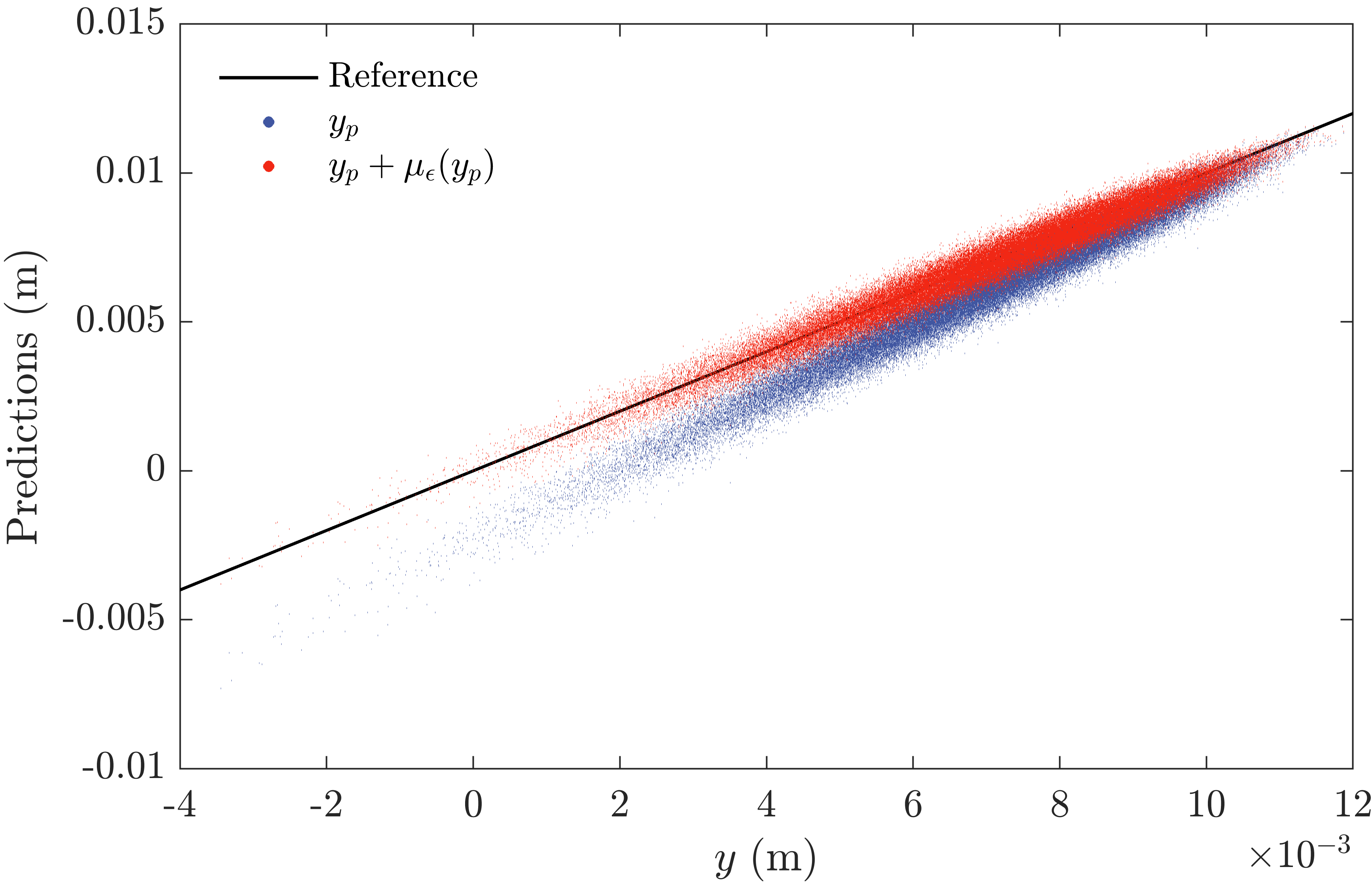
Figure 15: Response predictions of physics-based surrogate model and coupled physics-data-driven surrogate model for Example 3. The response prediction of the physics-based surrogate model $Y_{p}$ is highly correlated with the true responses $Y$, and the data-driven error correction corrects the bias. The estimated correlation coefficient between $Y$ and $Y_{p}$ as well as that between $Y$ and $Y_{p}+\mu_{\epsilon}(Y_{p})$ are both around $0.9815$. This is expected because Figure 13 is linear.

6 Conclusions

This paper develops an effective surrogate modeling method for rare event simulation with high-dimensional input uncertainties. The method circumvents the curse of dimensionality by using physics-based surrogate models parameterized by a few tunable parameters. A data-fitting error correction constructed in the output space of the physics-based surrogate model is leveraged to improve the bias of surrogate modeling. Due to inherent stochastic noise in the errors, the heteroscedastic Gaussian process is adopted to model the error correction. An active learning process is developed to effectively train the coupled physics-data-driven surrogate model to explore the critical region for the rare event. A final importance sampling step is designed to approximate the correction factor for the surrogate model-based probability estimation. Three numerical examples are studied to showcase the performance of the proposed method. The first example considers a static problem of a linear elastic cantilever beam with material properties represented by a Gaussian random field. The second example studies a dynamic problem of a nonlinear viscous damper under stochastic excitation. The third example investigates a multi-degree-of-freedom hysteretic system under stochastic excitation. Three schemes are investigated to construct physics-based surrogate models: a homogenization of material properties is considered in the first example, statistical linearization is used in the second example, and relaxation of the numerical solver is adopted in the third example. The numerical results are highly promising, suggesting that the proposed method can leverage limited calls of the original computational model to effectively estimate rare event probabilities with high-dimensional input uncertainties.

Appendix A Implementation details

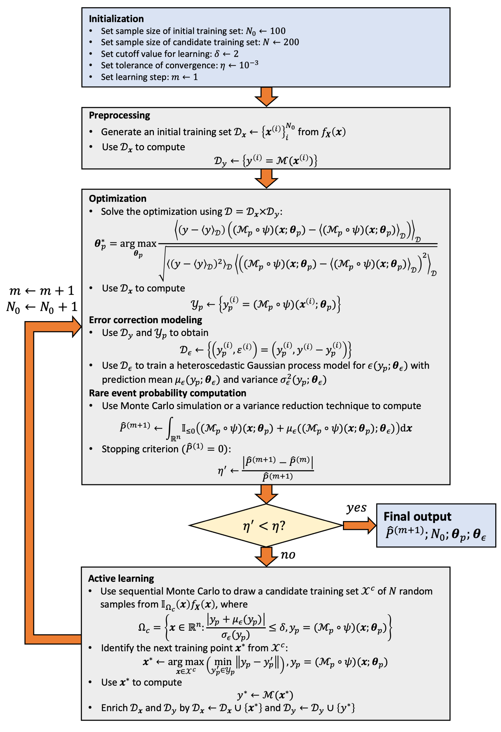
Figure 16: Training of the coupled physics-data-driven surrogate model.

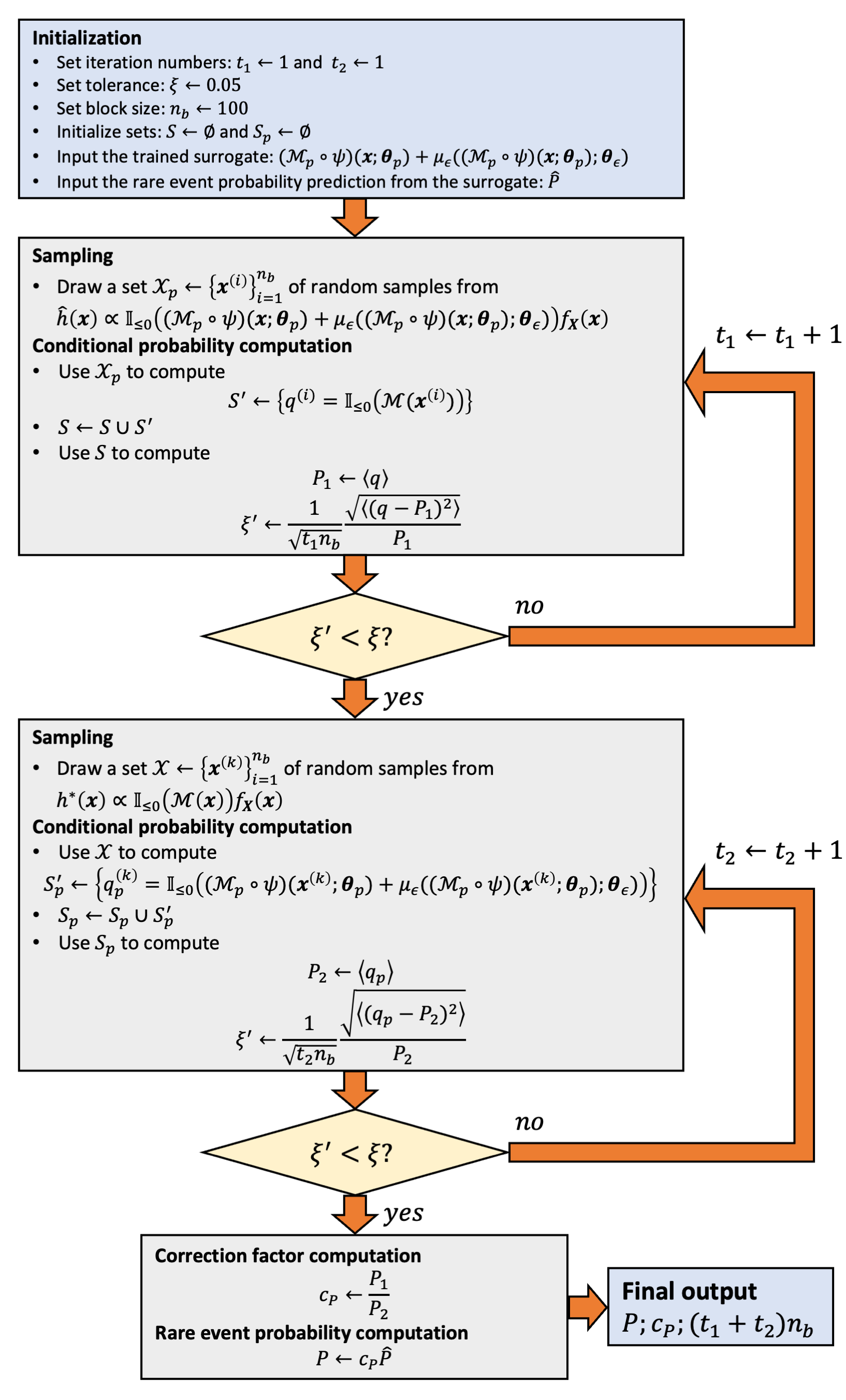
Figure 17: Importance sampling for the coupled physics-data-driven surrogate model.

References

- [1] Jérôme Morio and Mathieu Balesdent. Estimation of rare event probabilities in complex aerospace and other systems: a practical approach. Woodhead publishing, 2015.
- [2] Enrico Zio and Romney B Duffey. The risk of the electrical power grid due to natural hazards and recovery challenge following disasters and record floods: What next? In Climate Change and Extreme Events, pages 215–238. Elsevier, 2021.
- [3] Wen Jiang, Jason D Hales, Benjamin W Spencer, Blaise P Collin, Andrew E Slaughter, Stephen R Novascone, Aysenur Toptan, Kyle A Gamble, and Russell Gardner. Triso particle fuel performance and failure analysis with bison. Journal of Nuclear Materials, 548:152795, 2021.
- [4] Chao Dang and Jun Xu. A mixture distribution with fractional moments for efficient seismic reliability analysis of nonlinear structures. Engineering Structures, 208:109912, 2020.
- [5] Jun Xu, Long Li, and Zhao-Hui Lu. An adaptive mixture of normal-inverse gaussian distributions for structural reliability analysis. Journal of Engineering Mechanics, 148(3):04022011, 2022.
- [6] Jie Li and Jianbing Chen. Stochastic dynamics of structures. John Wiley & Sons, 2009.
- [7] Guohai Chen and Dixiong Yang. Direct probability integral method for stochastic response analysis of static and dynamic structural systems. Computer Methods in Applied Mechanics and Engineering, 357:112612, 2019.
- [8] Jianhua Xian, Cheng Su, and Houzuo Guo. Seismic reliability analysis of energy-dissipation structures by combining probability density evolution method and explicit time-domain method. Structural Safety, 88:102010, 2021.
- [9] Meng-Ze Lyu and Jian-Bing Chen. A unified formalism of the ge-gdee for generic continuous responses and first-passage reliability analysis of multi-dimensional nonlinear systems subjected to non-white-noise excitations. Structural Safety, 98:102233, 2022.
- [10] Reuven Y Rubinstein and Benjamin Melamed. Modern simulation and modeling, volume 7. Wiley New York, 1998.
- [11] David Landau and Kurt Binder. A guide to Monte Carlo simulations in statistical physics. Cambridge university press, 2015.
- [12] Siu-Kui Au and James L Beck. Estimation of small failure probabilities in high dimensions by subset simulation. Probabilistic engineering mechanics, 16(4):263–277, 2001.
- [13] Nolan Kurtz and Junho Song. Cross-entropy-based adaptive importance sampling using gaussian mixture. Structural Safety, 42:35–44, 2013.
- [14] Ziqi Wang and Junho Song. Cross-entropy-based adaptive importance sampling using von mises-fisher mixture for high dimensional reliability analysis. Structural Safety, 59:42–52, 2016.
- [15] Michael Engel, Oindrila Kanjilal, Iason Papaioannou, and Daniel Straub. Bayesian updating and marginal likelihood estimation by cross entropy based importance sampling. Journal of Computational Physics, 473:111746, 2023.
- [16] Mircea Grigoriu. Data-based importance sampling estimates for extreme events. Journal of Computational Physics, 412:109429, 2020.
- [17] Iason Papaioannou, Costas Papadimitriou, and Daniel Straub. Sequential importance sampling for structural reliability analysis. Structural safety, 62:66–75, 2016.
- [18] Ziqi Wang, Marco Broccardo, and Junho Song. Hamiltonian monte carlo methods for subset simulation in reliability analysis. Structural Safety, 76:51–67, 2019.
- [19] Jianhua Xian and Ziqi Wang. Relaxation-based importance sampling for structural reliability analysis. arXiv preprint arXiv:2303.13023, 2023.
- [20] Malur R Rajashekhar and Bruce R Ellingwood. A new look at the response surface approach for reliability analysis. Structural safety, 12(3):205–220, 1993.
- [21] DIEGO LORENZO Allaix and VINCENZO ILARIO Carbone. An improvement of the response surface method. Structural safety, 33(2):165–172, 2011.
- [22] Bruno Sudret and Armen Der Kiureghian. Comparison of finite element reliability methods. Probabilistic Engineering Mechanics, 17(4):337–348, 2002.
- [23] Emiliano Torre, Stefano Marelli, Paul Embrechts, and Bruno Sudret. Data-driven polynomial chaos expansion for machine learning regression. Journal of Computational Physics, 388:601–623, 2019.
- [24] Jorge E Hurtado. An examination of methods for approximating implicit limit state functions from the viewpoint of statistical learning theory. Structural Safety, 26(3):271–293, 2004.
- [25] Atin Roy and Subrata Chakraborty. Support vector machine in structural reliability analysis: A review. Reliability Engineering & System Safety, page 109126, 2023.
- [26] Irfan Kaymaz. Application of kriging method to structural reliability problems. Structural safety, 27(2):133–151, 2005.
- [27] Donald R Jones. A taxonomy of global optimization methods based on response surfaces. Journal of global optimization, 21:345–383, 2001.
- [28] Bruno Sudret. Meta-models for structural reliability and uncertainty quantification. arXiv preprint arXiv:1203.2062, 2012.
- [29] Barron J Bichon, Michael S Eldred, Laura Painton Swiler, Sandaran Mahadevan, and John M McFarland. Efficient global reliability analysis for nonlinear implicit performance functions. AIAA journal, 46(10):2459–2468, 2008.
- [30] Benjamin Echard, Nicolas Gayton, and Maurice Lemaire. Ak-mcs: an active learning reliability method combining kriging and monte carlo simulation. Structural Safety, 33(2):145–154, 2011.
- [31] Benjamin Echard, Nicolas Gayton, Maurice Lemaire, and Nicolas Relun. A combined importance sampling and kriging reliability method for small failure probabilities with time-demanding numerical models. Reliability Engineering & System Safety, 111:232–240, 2013.
- [32] Xiaoxu Huang, Jianqiao Chen, and Hongping Zhu. Assessing small failure probabilities by ak–ss: An active learning method combining kriging and subset simulation. Structural Safety, 59:86–95, 2016.
- [33] Ziqi Wang and Marco Broccardo. A novel active learning-based gaussian process metamodelling strategy for estimating the full probability distribution in forward uq analysis. Structural Safety, 84:101937, 2020.
- [34] Christos Lataniotis, Stefano Marelli, and Bruno Sudret. Extending classical surrogate modeling to high dimensions through supervised dimensionality reduction: a data-driven approach. International Journal for Uncertainty Quantification, 10(1), 2020.
- [35] Dimitris G Giovanis and Michael D Shields. Uncertainty quantification for complex systems with very high dimensional response using grassmann manifold variations. Journal of Computational Physics, 364:393–415, 2018.
- [36] Dimitris G Giovanis and Michael D Shields. Data-driven surrogates for high dimensional models using gaussian process regression on the grassmann manifold. Computer Methods in Applied Mechanics and Engineering, 370:113269, 2020.
- [37] Ketson R Dos Santos, Dimitrios G Giovanis, and Michael D Shields. Grassmannian diffusion maps–based dimension reduction and classification for high-dimensional data. SIAM Journal on Scientific Computing, 44(2):B250–B274, 2022.
- [38] Katiana Kontolati, Dimitrios Loukrezis, Dimitrios G Giovanis, Lohit Vandanapu, and Michael D Shields. A survey of unsupervised learning methods for high-dimensional uncertainty quantification in black-box-type problems. Journal of Computational Physics, 464:111313, 2022.
- [39] Zhongming Jiang and Jie Li. High dimensional structural reliability with dimension reduction. Structural Safety, 69:35–46, 2017.
- [40] Tong Zhou and Yongbo Peng. Active learning and active subspace enhancement for pdem-based high-dimensional reliability analysis. Structural Safety, 88:102026, 2021.
- [41] N Navaneeth and Souvik Chakraborty. Surrogate assisted active subspace and active subspace assisted surrogate—a new paradigm for high dimensional structural reliability analysis. Computer Methods in Applied Mechanics and Engineering, 389:114374, 2022.
- [42] Jungho Kim, Ziqi Wang, and Junho Song. Adaptive active subspace-based metamodeling for high-dimensional reliability analysis. arXiv preprint arXiv:2304.06252, 2023.
- [43] Zhong-ming Jiang, De-Cheng Feng, Hao Zhou, and Wei-Feng Tao. A recursive dimension-reduction method for high-dimensional reliability analysis with rare failure event. Reliability Engineering & System Safety, 213:107710, 2021.
- [44] Maziar Raissi, Paris Perdikaris, and George E Karniadakis. Physics-informed neural networks: A deep learning framework for solving forward and inverse problems involving nonlinear partial differential equations. Journal of Computational physics, 378:686–707, 2019.
- [45] Yinhao Zhu, Nicholas Zabaras, Phaedon-Stelios Koutsourelakis, and Paris Perdikaris. Physics-constrained deep learning for high-dimensional surrogate modeling and uncertainty quantification without labeled data. Journal of Computational Physics, 394:56–81, 2019.
- [46] Kevin Linka, Amelie Schäfer, Xuhui Meng, Zongren Zou, George Em Karniadakis, and Ellen Kuhl. Bayesian physics informed neural networks for real-world nonlinear dynamical systems. Computer Methods in Applied Mechanics and Engineering, 402:115346, 2022.
- [47] Zeng Meng, Qiaochu Qian, Mengqiang Xu, Bo Yu, Ali Rıza Yıldız, and Seyedali Mirjalili. Pinn-form: A new physics-informed neural network for reliability analysis with partial differential equation. Computer Methods in Applied Mechanics and Engineering, 414:116172, 2023.
- [48] Benjamin Peherstorfer, Karen Willcox, and Max Gunzburger. Survey of multifidelity methods in uncertainty propagation, inference, and optimization. Siam Review, 60(3):550–591, 2018.
- [49] Benjamin Peherstorfer, Tiangang Cui, Youssef Marzouk, and Karen Willcox. Multifidelity importance sampling. Computer Methods in Applied Mechanics and Engineering, 300:490–509, 2016.
- [50] Boris Kramer, Alexandre Noll Marques, Benjamin Peherstorfer, Umberto Villa, and Karen Willcox. Multifidelity probability estimation via fusion of estimators. Journal of Computational Physics, 392:385–402, 2019.
- [51] John W Peterson, Alexander D Lindsay, and Fande Kong. Overview of the incompressible navier–stokes simulation capabilities in the moose framework. Advances in Engineering Software, 119:68–92, 2018.
- [52] Zhong-Hua Han, Stefan Görtz, and Ralf Zimmermann. Improving variable-fidelity surrogate modeling via gradient-enhanced kriging and a generalized hybrid bridge function. Aerospace Science and technology, 25(1):177–189, 2013.
- [53] Isaac M Held. The gap between simulation and understanding in climate modeling. Bulletin of the American Meteorological Society, 86(11):1609–1614, 2005.
- [54] Stephen H Crandall. A half-century of stochastic equivalent linearization. Structural Control and Health Monitoring: The Official Journal of the International Association for Structural Control and Monitoring and of the European Association for the Control of Structures, 13(1):27–40, 2006.
- [55] Isaac Elishakoff and Stephen H Crandall. Sixty years of stochastic linearization technique. Meccanica, 52:299–305, 2017.
- [56] Ziqi Wang. Optimized equivalent linearization for random vibration. arXiv preprint arXiv:2208.08991, 2022.
- [57] Somayajulu LN Dhulipala, Michael D Shields, Benjamin W Spencer, Chandrakanth Bolisetti, Andrew E Slaughter, Vincent M Labouré, and Promit Chakroborty. Active learning with multifidelity modeling for efficient rare event simulation. Journal of Computational Physics, 468:111506, 2022.
- [58] Somayajulu LN Dhulipala, Michael D Shields, Promit Chakroborty, Wen Jiang, Benjamin W Spencer, Jason D Hales, Vincent M Laboure, Zachary M Prince, Chandrakanth Bolisetti, and Yifeng Che. Reliability estimation of an advanced nuclear fuel using coupled active learning, multifidelity modeling, and subset simulation. Reliability Engineering & System Safety, 226:108693, 2022.
- [59] Miguel Lázaro-Gredilla, Michalis K Titsias, Jochem Verrelst, and Gustavo Camps-Valls. Retrieval of biophysical parameters with heteroscedastic gaussian processes. IEEE Geoscience and Remote Sensing Letters, 11(4):838–842, 2013.
- [60] TJ Rogers, P Gardner, N Dervilis, K Worden, AE Maguire, E Papatheou, and EJ Cross. Probabilistic modelling of wind turbine power curves with application of heteroscedastic gaussian process regression. Renewable Energy, 148:1124–1136, 2020.
- [61] Jungho Kim, Sang-ri Yi, and Junho Song. Estimation of first-passage probability under stochastic wind excitations by active-learning-based heteroscedastic gaussian process. Structural Safety, 100:102268, 2023.
- [62] Jan Hauke and Tomasz Kossowski. Comparison of values of pearson’s and spearman’s correlation coefficients on the same sets of data. Quaestiones geographicae, 30(2):87–93, 2011.
- [63] Søren Taverniers, Eric J Hall, Markos A Katsoulakis, and Daniel M Tartakovsky. Mutual information for explainable deep learning of multiscale systems. Journal of Computational Physics, 444:110551, 2021.
- [64] Samir Beneddine. Nonlinear input feature reduction for data-based physical modeling. Journal of Computational Physics, 474:111832, 2023.
- [65] Andrew R Conn, Katya Scheinberg, and Luis N Vicente. Introduction to derivative-free optimization. SIAM, 2009.
- [66] Vincent Dubourg, Bruno Sudret, and Jean-Marc Bourinet. Reliability-based design optimization using kriging surrogates and subset simulation. Structural and Multidisciplinary Optimization, 44:673–690, 2011.
- [67] Maliki Moustapha, Stefano Marelli, and Bruno Sudret. Active learning for structural reliability: Survey, general framework and benchmark. Structural Safety, 96:102174, 2022.
- [68] Radford M Neal et al. Mcmc using hamiltonian dynamics. Handbook of markov chain monte carlo, 2(11):2, 2011.
- [69] Iason Papaioannou, Wolfgang Betz, Kilian Zwirglmaier, and Daniel Straub. Mcmc algorithms for subset simulation. Probabilistic Engineering Mechanics, 41:89–103, 2015.
- [70] Masanobu Shinozuka and George Deodatis. Simulation of stochastic processes by spectral representation. Applied Mechanics Reviews, 44(4):191–204, 1991.
- [71] Jianhua Xian, Cheng Su, and Billie F Spencer Jr. Stochastic sensitivity analysis of energy-dissipating structures with nonlinear viscous dampers by efficient equivalent linearization technique based on explicit time-domain method. Probabilistic Engineering Mechanics, 61:103080, 2020.
- [72] YK Wen. Equivalent linearization for hysteretic systems under random excitation. Journal of Applied Mechanics, 47(1):150–154, 1980.