Unleash Data Generation for Efficient and Effective Data-free Knowledge Distillation

Abstract

Data-Free Knowledge Distillation (DFKD) has recently made remarkable advancements with its core principle of transferring knowledge from a teacher neural network to a student neural network without requiring access to the original data. Nonetheless, existing approaches encounter a significant challenge when attempting to generate samples from random noise inputs, which inherently lack meaningful information. Consequently, these models struggle to effectively map this noise to the ground-truth sample distribution, resulting in the production of low-quality data and imposing substantial time requirements for training the generator. In this paper, we propose a novel Noisy Layer Generation method (NAYER) which relocates the randomness source from the input to a noisy layer and utilizes the meaningful label-text embedding (LTE) as the input. The significance of LTE lies in its ability to contain substantial meaningful inter-class information, enabling the generation of high-quality samples with only a few training steps. Simultaneously, the noisy layer plays a key role in addressing the issue of diversity in sample generation by preventing the model from overemphasizing the constrained label information. By reinitializing the noisy layer in each iteration, we aim to facilitate the generation of diverse samples while still retaining the method’s efficiency, thanks to the ease of learning provided by LTE. Experiments carried out on multiple datasets demonstrate that our NAYER not only outperforms the state-of-the-art methods but also achieves speeds 5 to 15 times faster than previous approaches.

1 Introduction

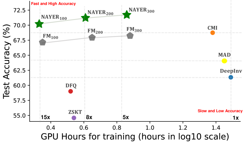
Figure 1: Accuracy of student models and GPU hours of training time on CIFAR-100 dataset. All variants of our method NAYER not only attains the highest accuracies across but also accelerates the training process by 5 to 15 times compared to DeepInv (Yin et al., 2020).

Knowledge distillation (KD) aims to train a student model capable of emulating the capabilities of a pre-trained teacher model. Over the past decade, KD has been explored across diverse domains, including image recognition (Qiu et al., 2022), speech recognition (Yoon et al., 2021), and natural language processing (Sanh et al., 2019). Conventional KD methods generally assume that the student model has access to all or part of the teacher’s training data. However, real-world applications often impose constraints on accessing the original training data. This issue becomes particularly relevant in cases involving privacy-sensitive medical data, which may contain personal information or data considered proprietary by vendors. Consequently, in such contexts, conventional KD methods no longer suffice to address the challenges posed.

Data-Free Knowledge Distillation (DFKD) has recently seen significant advancements as an alternative method. Its core principle involves transferring knowledge from a teacher neural network ($\mathcal{T}$) to a student neural network ($\mathcal{S}$) by generating synthetic data instead of accessing the original training data. The synthetic data enable adversarial training of the generator and student (Nayak et al., 2019; Micaelli & Storkey, 2019). In this setup, the student seeks to match the teacher’s predictions on synthetic data, while the generator aims to create samples that maximize the discrepancy between the student’s and teacher’s predictions (Fig. 2a).

Due to its reliance on synthetic samples, the need for an effective and efficient data-free generation technique becomes imperative. A major limitation of current DKFD methods is that they merely generate synthetic samples from random noise, neglecting to incorporate supportive and semantic information (Binici et al., 2022a; Fang et al., 2022; Yu et al., 2023; Patel et al., 2023). This limitation in turn incurs the generation of low-quality data and excessive time requirements for training the generator, rendering them unsuitable for large-scale tasks. Notably, almost SOTA DFKD methods do not report results on large-scale ImageNet due to the significant training time involved. Even with smaller datasets such as CIFAR-100 (see Fig. 1), state-of-the-art DFKD methods such as CMI (Fang et al., 2021), MAD (Do et al., 2022), or DeepInv still demand approximately 25 to 30 hours of training while struggling to achieve high accuracy. This emphasizes the pressing need for more efficient and effective DFKD techniques.

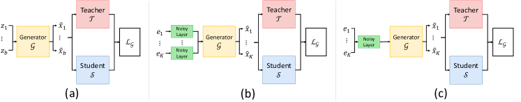
Figure 2: Data Generation Strategies: (a) The classic Data-free Generation, which optimizes random noise (z); (b) the 1-to-1 Noisy Layer Generation, which uses one noisy layer for generating one synthetic image from the embedding of label’s text (${\bm{e}}_{{\bm{y}}}$) by CLIP (Radford et al., 2021); (c) K-to-1 Noisy Layer Generation, which uses one noisy layer to generate multiple synthetic images.

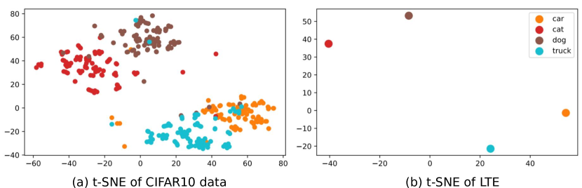
Figure 8: t-SNE Visualization of Label-Text Embedding and Ground-Truth Dataset Distribution for Four Classes: Car, Cat, Dog, and Truck.

In this paper, we introduce a simple yet effective DFKD method called Noisy LAYER Generation (NAYER). Our approach relocates the source of randomness from the input to the noisy layer and utilizes the meaningful label-text embedding (LTE) generated by a pretrained text encoder (Radford et al., 2021) as the input. In this context, LTE plays a crucial role in accelerating the training process due to its ability to encapsulate useful interclass information. It is noteworthy that in the field of text embedding, there is a common observation that the text with similar meanings tend to exhibit closer embedding proximity to one another (Le & Mikolov, 2014). As can be seen in Fig. 8, in Fig. 8, our empirical observations reveal a close alignment between the proximity pattern in LTE and that of the ground-truth data. Consequently, by using LTE as input, our approach can proficiently generate high-quality samples that closely mimic the distributions of their respective classes with only a few training steps, as illustrated in Fig. 5a.

However, when utilizing LTE as the input, we empirically observed that the generation process in existing methods suffers from a form of mode collapse, meaning that the generator consistently produces similar data in every iteration. We attribute this phenomenon to an overemphasis on constant label-related information. This can be demonstrated when we concatenate LTE with random noise to study the weight magnitudes of both, indicative of their significance in learning (Frankle & Carbin, 2018). Fig. 3d illustrates that weight magnitudes for learning LTE notably exceed those for random noise, indicating the model’s excessive emphasis on label information compared to random noise. This emphasis might inadvertently overshadow the crucial random noise component necessary for generating a diverse array of samples.

Our solution addresses this issue by relocating the source of randomness from the input to the layer level by adding a noisy layer to learn the constant label information. This involves incorporating a random noise layer to function as an intermediary between the generator and LTE, which prevents the generator from relying solely on unchanging label information (Fig. 2b). The source of randomness now comes from the random reinitialization of the noisy layer for each iteration. Through this mechanism, we aim to effectively mitigate the risk of overemphasizing label information, thus enhancing the diversity of synthesized images. Furthermore, thanks to the inherent ease of learning label-text embeddings, regardless of how it is initialized, the noisy layer can consistently generate high-quality samples in just a few steps, thereby maintaining the method’s efficiency. Additionally, we propose leveraging a single noisy layer to generate multiple samples (e.g., 100 images across 100 classes of CIFAR-100) (Fig. 2c). This strategy capitalizes on the multiple gradient sources stemming from various classes, enhancing the diversity of the noisy layer’s output, reducing model size and expediting the training process.

We conducted comprehensive experiments on several datasets, including ImageNet, demonstrating the superiority of our proposed techniques over state-of-the-art algorithms. Notably, NAYER not only outperforms the existing state-of-the-art approaches in terms of accuracy but also exhibits remarkable speed enhancements. Specifically, as illustrated in Fig. 1, our proposed methods achieve speeds that are 5 to even 15 times faster while also attaining higher accuracies compared to previous methods, highlighting their efficiency and effectiveness.

2 Related Work

Data-Free Knowledge Distillation. DFKD methods generate synthetic images to transfer knowledge from a pre-trained teacher model to a student model. These data are used to jointly train the generator and the student in an adversarial manner (Nayak et al., 2019; Micaelli & Storkey, 2019). Under this adversarial learning scheme, the student attempts to make predictions close to the teacher’s on synthetic data, while the generator tries to create samples that maximize the mismatch between the student’s and the teacher’s predictions. This adversarial game enables a rapid exploration of synthetic distributions useful for knowledge transfer between the teacher and the student.

Data-Free Generation. As the central principle of DFKD revolves around synthetic samples, the data-free generation technique plays a pivotal role. (Yin et al., 2020) proposes the image-optimized method which attempts to optimize the random noise images using teacher network batch normalization statistics. Sample-optimized methods (Fang et al., 2021; Yu et al., 2023) focus on optimizing random noise over numerous training steps to produce synthetic images in case-by-case strategy. In contrast, generator-optimized methods (Do et al., 2022; Patel et al., 2023; Binici et al., 2022a) attempt to ensure that the generator has the capacity to comprehensively encompass the entire distribution of the original data. In the other words, regardless of the input random noise, these methods aim to consistently yield high-quality samples for training the student model. This approach often prolongs the training process and may not consistently produce high-quality samples, particularly when diverse noises are employed during both the sampling and training phases. Furthermore, the main problem in existing data-free generation is the use of random noise input without any meaningful information, leading to generate the low-quality samples and prolonged training times for the generator. (Fang et al., 2022) introduced FM, a method incorporating a meta generator to accelerate the DFKD process significantly. However, this acceleration comes at the cost of a noticeable trade-off in classification accuracy.

Synthetizing Samples from Label Information. Drawing inspiration from the success of incorporating label information in adversarial frameworks like Conditional GAN (Mirza & Osindero, 2014), several methods in DFKD have adopted strategies to generate images guided by labels. In these approaches, a common practice involves fusing random noise (${\bm{z}}$) with a learnable embedding (${\bm{e}}_{\bm{y}}$) of the one-hot label vector, which is used as input for the model (Luo et al., 2020; Yoo et al., 2019; Do et al., 2022). This combination enhances control over the resulting class-specific synthetic images. However, despite the potential of label information, its application has yielded only minor improvements. This can be attributed to two key factors. Firstly, the one-hot vector introduces sparse information that merely distinguishes labels uniformly, failing to capture the nuanced relationships between different classes. Consequently, the model struggles to generate images that align closely with ground-truth distributions. Secondly, there exists a challenge in balancing the generated images’ quality and diversity when incorporating label information. This can inadvertently lead to an overemphasis on label-related details, potentially overshadowing the crucial contribution of random noise, which is necessary for generating a diverse range of samples.

3 Proposed Method

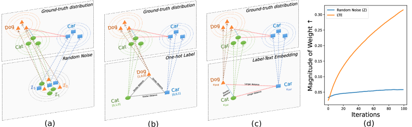
Figure 3: (a) Random noise for data generation. (b) One-hot labels only uniformly distinguish labels, lacking inter-class relationships. In contrast, (c) LTE captures inter-class connections, bringing similar classes closer in the embedding space. This proximity enhances the similarity between the input and ground-truth sample distributions, thereby allowing the model to more easily mimic the ground-truth distribution and accelerating the learning process. (d) The averaging magnitude of weight used to learn LTE is much larger than those for random noise, highlighting the model’s negative focus on label information while ignoring random noise.

3.1 Data-free Knowledege Distillation Framework

Consider a training dataset $D=\{({\bm{x}}_{i},{\bm{y}}_{i})\}_{i=1}^{m}$ with ${\bm{x}}_{i}\in\mathbb{R}^{c\times h\times w}$ and ${\bm{y}}_{i}\in\{1,2,\cdots,K\}$, where the pair $({\bm{x}}_{i},{\bm{y}}_{i})$ represents a training sample and its corresponding label, respectively. Let $\mathcal{T}=\mathcal{T}_{\theta_{\mathcal{T}}}$ be a pre-trained teacher network on $D$. The objective of DFKD is to train a student network $\mathcal{S}=\mathcal{S}_{\theta_{\mathcal{S}}}$ to emulate $\mathcal{T}$’s performance, all without needing access to the original dataset $D$. To achieve this, common DFKD techniques utilize a lightweight generator ($\mathcal{G}=\mathcal{G}_{\theta_{\mathcal{G}}}$) to create synthetic images. These images are then used to train the student network $\mathcal{S}$, employing random noise ${\bm{z}}$ as a key element in the process. This noise is typically drawn from a standard Gaussian distribution $\mathcal{N}(\bm{0},\mathbf{I})$, and it plays a crucial role in generating diverse synthetic samples for training.

Nayak et al. (2019) introduces an adversarial mechanism to concurrently train the generator ($\mathcal{G}$) and the student ($\mathcal{S}$) through the optimization of min-max objective functions. Specifically, for the synthetic images $\hat{{\bm{x}}}=\mathcal{G}({\bm{z}})$, the student network $\mathcal{S}$ is optimized to minimize the discrepancy between its predictions $\mathcal{S}(\hat{{\bm{x}}})$ and those of the teacher $\mathcal{T}(\hat{{\bm{x}}})$ (Eq. 1). This optimization process enables alignment between the student’s output and the teacher’s expertise, facilitating effective knowledge transfer.

$$\min\limits_{\theta_{\mathcal{S}}}\mathcal{L}_{\mathcal{S}}\triangleq\mathbb{E}_{\hat{{\bm{x}}}\sim\mathcal{G}({\bm{z}})}\Big{[}\mathcal{L}_{\text{KL}}(\mathcal{T}(\hat{{\bm{x}}}),\mathcal{S}(\hat{{\bm{x}}}))\Big{]},$$ (1)

where $\mathcal{L}_{\text{KL}}$ denotes the Kullback-Leibler divergence. Let $\mathcal{U}(K)$ be a uniform distribution over $\{1,\cdots,K\}$, $\alpha_{cls},\alpha_{adv}$ and $\alpha_{bn}$ be hyperparameters of the algorithm. The generator ($\mathcal{G}$) then minimizes $\mathcal{L}_{\mathcal{G}}$ defined as in Eq. (2).

$$\leavevmode\resizebox{365.68546pt}{}{$\min\limits_{\theta_{\mathcal{G}}}\mathcal{L}_{\mathcal{G}}\triangleq\mathbb{E}_{{\bm{z}}\sim\mathcal{N}(0,\text{I}),\hat{{\bm{x}}}\sim\mathcal{G}({\bm{z}}),\hat{{\bm{y}}}\sim\mathcal{U}(K)}\Big{[}\alpha_{cls}\mathcal{L}_{\text{CE}}(\mathcal{T}(\hat{{\bm{x}}}),\hat{{\bm{y}}})-\alpha_{adv}\mathcal{L}_{\text{KL}}(\mathcal{T}(\hat{{\bm{x}}}),\mathcal{S}(\hat{{\bm{x}}}))+\alpha_{bn}\mathcal{L}_{\text{BN}}(\mathcal{T}(\hat{{\bm{x}}}))\Big{]}$}.$$ (2)

Within this context, $\mathcal{L}_{\text{CE}}$ represents the Cross-Entropy loss term, serving the purpose of training the student on images residing within the high-confidence region of the teacher’s knowledge. Conversely, the negative $\mathcal{L}_{\text{KL}}$ term facilitates the exploration of synthetic distributions, boosting effective knowledge transfer between the teacher and the student. In other words, the student network takes on a role as a discriminator in GANs, ensuring the generator is geared towards producing images that the teacher has mastered, yet the student network has not previously learned. This approach facilitates the focused development of the student’s understanding in areas where it lags behind the teacher, enhancing the overall knowledge transfer process. We also use batch norm regularization ($\mathcal{L}_{\text{BN}}$) (Yin et al., 2020; Fang et al., 2022), a commonly used loss in DFKD, to constrain the mean and variance of the feature at the batch normalization layer to be consistent with the running-mean and running-variance of the same layer.

3.2 Data-free Generation based on Label-Text Embedding

To achieve rapid convergence and generate high-quality images, we introduce an innovative strategy that leverages the concept of label-text embeddings (LTE) as an input. Given the batch of $b$ target classes $\hat{{\bm{y}}}=[\hat{{\bm{y}}}_{1},\cdots,\hat{{\bm{y}}}_{b}]$, their label text $Y_{\hat{{\bm{y}}}}=[Y_{\hat{{\bm{y}}}_{1}},\cdots,Y_{\hat{{\bm{y}}}_{b}}]$ is embedded using a pretrained text encoder $\mathcal{C}=\mathcal{C}_{\theta_{\mathcal{C}}}$, followed by batch normalization to facilitate easier discrimination.

$${\bm{e}}_{\hat{{\bm{y}}}}=\text{BatchNorm}(\mathcal{C}(Y_{\hat{{\bm{y}}}}))$$ (3)

In this approach, we employ CLIP (Radford et al., 2021) as the encoder and conduct experiments related to this choice, which are detailed in Table 9. Several studies suggest that text embedding enjoys the tendency for text with similar meanings to exhibit proximity in their embeddings (Le & Mikolov, 2014). Fig. 3a-c visually represents the LTE, highlighting their superior capacity to depict the relationship between the ‘Dog’ and ‘Cat’ classes. This is evident in their closer proximity (shorter distance) when compared to the ‘Car’ class. This visualization emphasizes the effectiveness of LTE in capturing inherent connections among different classes, in contrast to random noise or one-hot vectors, thereby providing valuable insights into inter-class relationships. This characteristic of LTE contributes to making the input distribution (representing labels) and ground-truth distribution (representing actual data) more similar. As a result, it facilitates the model’s mapping between these two distributions, accelerating the learning process. Our approach employs LTE as the input for the generator, eliminating the reliance on random noise for synthetic image generation. It is important to note that the embedding ${\bm{e}}_{\hat{{\bm{y}}}}$ will remain fixed throughout the entire training process.

$$\hat{{\bm{x}}}=\mathcal{G}({\bm{e}}_{\hat{{\bm{y}}}})$$ (4)

Moreover, the synthetic images $\hat{{\bm{x}}}=\mathcal{G}({\bm{e}}_{\hat{{\bm{y}}}})$ are used in Eq. (1) and Eq. (2) to train the student $\mathcal{S}$ and the generator $\mathcal{G}$. Specifically, we regularly reinitialize the generator $\mathcal{G}$ at specified intervals to generate more diverse images. Thanks to the informative content embedded in LTE, our approach can efficiently produce high-quality samples with minimal computational steps. We have also conducted an ablation study to substantiate this claim, as illustrated in Fig. 5a-c. The results of this study highlight that LTE significantly accelerates convergence in terms of Cross-Entropy (CE) Loss and yields higher-quality images (as measured by the Inception Score or IS score) in comparison to random noise and one-hot vectors. This acceleration empowers our method to achieve convergence with a considerably smaller number of generator training steps (30 steps for CIFAR10 and 40 steps for CIFAR100), as opposed to the 2,000 steps required by DeepInv or the 500 steps of CMI, all while maintaining superior accuracy (as detailed in Table 1).

3.3 Generating Diverse Samples with Noisy Layer

While leveraging label information provides valuable advantages for data generation including (i) accelerating the convergence rate of the CE loss (see Fig. 5a) and (ii) improving the quality of the synthetic images with a higher Inception Score (see Fig. 5b), the synthetic images are less diverge as shown in Fig. 5c. A naive approach is to incorporate the source of randomness ${\bm{z}}\sim\mathcal{N}(\bm{0},\mathbf{I})$ into the LTE $e_{\hat{{\bm{y}}}}$ (i.e., $\hat{{\bm{x}}}=\mathcal{G}({\bm{e}}_{\hat{{\bm{y}}}},{\bm{z}})$). Unfortunately, we empirically observed that the generator consistently produces similar data in every iteration (see Fig. 5f). We attribute this issues to the risk of overemphasizing label-related information, potentially overshadowing the essential random noise component necessary for generating a diverse range of samples. To illustrate this concern, we examine the magnitudes of the weights involved in learning the concatenation of $({\bm{e}}_{\hat{{\bm{y}}}},{\bm{z}})$, which can be seen as the significance of these weights (Frankle & Carbin, 2018). As depicted in Fig. 3d, our findings reveal the average weight magnitudes used for learning LTE are significantly larger than those associated with random noise. This observation underscores the model’s tendency to overemphasize label information, while neglecting the importance of random noise.

To address this challenge, we propose a solution that involves repositioning the source of randomness from the input level to the layer level. This is achieved by introducing a noisy layer, responsible for learning the constant LTE input. By incorporating the noise layer as an intermediary between the generator and LTE, we ensure that the generator does not solely rely on unchanging label information. The source of randomness now derives from the random reinitialization of the noisy layer during each iteration. Through this mechanism, our goal is to effectively mitigate the risk of an negatively emphasis on LTE, thus enhancing the diversity of the synthesized images. Furthermore, thanks to the ease of training LTE, regardless of their initialization, the noisy layer consistently produces high-quality samples within a few iterations, thereby maintaining the method’s efficiency (see Fig. 5d-f). Given LTEs ${\bm{e}}_{\hat{{\bm{y}}}}$, we feed these ${\bm{e}}_{\hat{{\bm{y}}}}$ into the noisy layer $\mathcal{Z}_{\theta_{\mathcal{Z}}}\sim\mathcal{N}(0,\text{I})$. Then, the output of the noisy layer is fed into the generator $\mathcal{G}$ to produce the batch of synthetic images $\hat{{\bm{x}}}$:

$$\hat{{\bm{x}}}=\mathcal{G}(\mathcal{Z}({\bm{e}}_{\hat{{\bm{y}}}}))$$ (5)

To achieve the most straightforward architecture, $\mathcal{Z}\in\mathbb{R}^{e\times r}$ is designed as a single linear layer with an input size equal to the embedding size of the text encoder ($e$) and an output size of the noise dimension ($r$). Typically, the output size is set to 1,000, in line with previous works (Patel et al., 2023; Do et al., 2022). In our method, we employ a single noisy layer designed to learn from all available classes (K-to-1) (i.e., inputting ${\bm{e}}_{\hat{{\bm{y}}}}$ with $\hat{{\bm{y}}}=1,\dots,K$ to a single noisy layer $\mathcal{Z}$), meaning that we need $M$ noisy layers if we wish to generate $MK$ synthetic images simultaneously. This design allows the noisy layer to generate multiple samples simultaneously, like 100 for CIFAR100 or 10 for CIFAR10, thus efficiently expediting training. This strategy harnesses multiple gradient sources from diverse classes, enriching the diversity of the noisy layer’s output. Moreover, it leads to a reduction in model size and accelerates the training process. Our ablation study (Fig. 5d-f) demonstrated that using a single noisy layer to synthesize a batch of images (K-to-1) significantly enhances generator diversity, ensuring both fast convergence and high-quality sample generation.

3.4 Method Summary

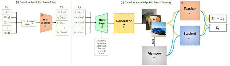
Figure 4: General Architecture of Noisy Layer Generation for Data-free Knowledge Distillation.

Input: Pretrained teacher $\mathcal{T}_{\theta_{\mathcal{T}}}$, student $\mathcal{S}_{\theta_{\mathcal{S}}}$, generator $\mathcal{G}_{\theta_{\mathcal{G}}}$, text encoder $\mathcal{C}_{\theta_{\mathcal{C}}}$, list of labels $\hat{{\bm{y}}}$ and list of text of these labels $Y_{\hat{{\bm{y}}}}$;

Output: An optimized student $\mathcal{S}_{\theta_{\mathcal{S}}}$

1 ${\bm{e}}_{\hat{{\bm{y}}}}=BatchNorm(\mathcal{C}(Y_{\hat{{\bm{y}}}}))$;

2 for $\mathcal{E}$ epochs do

3       for $I$ iterations do

4             Randomly reinitializing noisy layers $\mathcal{Z}_{\theta_{\mathcal{Z}}}\sim\mathcal{N}(0,\text{I})$ for each iteration;

5             for $g$ steps do

6                   $\hat{{\bm{x}}}\leftarrow\mathcal{G}(\mathcal{Z}({\bm{e}}_{\hat{{\bm{y}}}}))$;

7                   $\mathcal{L}_{\mathcal{Z}}\leftarrow\alpha_{cls}\mathcal{L}_{\text{CE}}(\mathcal{T}(\hat{{\bm{x}}}),\hat{{\bm{y}}})-\alpha_{adv}\mathcal{L}_{\text{KL}}(\mathcal{T}(\hat{{\bm{x}}}),\mathcal{S}(\hat{{\bm{x}}}))+\alpha_{bn}\mathcal{L}_{\text{BN}}(\mathcal{T}(\hat{{\bm{x}}}))$;

8                   Update $\theta_{\mathcal{G}},\theta_{\mathcal{Z}}$ by minimizing $\mathcal{L}_{\mathcal{Z}}$;

9             end for

10            $\mathcal{M}\leftarrow\mathcal{M}\cup\hat{{\bm{x}}}$;

11            

12       end for

13      for $S$ iterations do

14             $\hat{{\bm{x}}}\sim\mathcal{M}$;

15             Update $\theta_{\mathcal{S}}$ by minimizing $\mathcal{L}_{\mathcal{S}}\leftarrow\mathcal{L}_{\text{KL}}(\mathcal{T}(\hat{{\bm{x}}}),\mathcal{S}(\hat{{\bm{x}}}))$;

16       end for

17      

18 end for

Algorithm 1 NAYER

The comprehensive architecture of our method is visually depicted in Fig. 4, while the detailed pseudo code is presented in Algorithm 1. NAYER initially embeds the label text of each class using a text encoder. It is important to note that the embedding will remain fixed throughout the entire training process. Subsequently, our method undergoes training for $\mathcal{E}$ epochs. Within each epoch, NAYER consists of two distinct phases. The first phase involves training the generator. In each iteration $I$, as described in Algorithm 1, the noisy layer $\mathcal{Z}$ is reinitialized (line 4) before being utilized to learn the LTE. The generator and the noisy layer are then trained through $g$ steps using Eq. (6) to optimize their performance (line 8).

(6)

The second phase involves training the student networks. During this phase, all the generated samples are stored in the memory module $\mathcal{M}$ to mitigate the risk of forgetting (line 10), following a similar approach as outlined in Fang et al. (2022). Ultimately, the student model is trained by Eq. (7) over $S$ iterations, utilizing the samples from $\mathcal{M}$ (lines 13 and 14).

$$\min\limits_{\theta_{\mathcal{S}}}\mathcal{L}_{\mathcal{S}}\triangleq\mathbb{E}_{\hat{{\bm{x}}}\sim\mathcal{M}}\Big{[}\mathcal{L}_{\text{KL}}(\mathcal{T}_{\theta_{\mathcal{T}}}(\hat{{\bm{x}}}),\mathcal{S}_{\theta_{\mathcal{S}}}(\hat{{\bm{x}}}))\Big{]}$$ (7)

4 Experiments

4.1 Experimental Settings

We conducted a comprehensive evaluation of our method across various backbone networks, namely ResNet (He et al., 2016), VGG (Simonyan & Zisserman, 2014), and WideResNet (WRN)(Zagoruyko & Komodakis, 2016), spanning three distinct classification datasets: CIFAR10, CIFAR100 (Krizhevsky et al., 2009), and Tiny-ImageNet (Le & Yang, 2015). The datasets feature varying scales and complexities, offering a well-rounded assessment of our method’s capabilities. In detail, CIFAR10 and CIFAR100 encompass a total of 60,000 images, partitioned into 50,000 for training and 10,000 for testing. CIFAR10 comprises 10 categories, while CIFAR100 boasts 100 categories. The images within both datasets are characterized by a resolution of 32×32 pixels. On the other hand, Tiny-ImageNet comprises 100,000 training images and 10,000 validation images, with a higher resolution of 64 × 64 pixels. This dataset encompasses a diverse array of 200 image categories, contributing to the breadth and comprehensiveness of our evaluation.

4.2 Results and Analysis

Comparison with SOTA DFKD Methods. Table 1 displays the results of DFKD achieved by our methods and several state-of-the-art (SOTA) approaches. In general, previous methods exhibit limitations when generating images from random noise, impacting both training time and image diversity. By using LTE as the input and relocating the source of randomness from the input to the layer level, our approach provides highly diverse training images and faster running time. Notably, with 300 epochs, our method achieves SOTA performance in all comparison cases, except for the Resnet32/Resnet18 case in CIFAR10. However, it is essential to note that our method was designed in a straightforward manner, without incorporating innovative techniques found in current SOTA approaches, such as activation region constraints and feature exchange in SpaceshipNet (Yu et al., 2023), knowledge acquisition and retention meta-learning in KAKR (Patel et al., 2023), and momentum distillation in MAD (Do et al., 2022).

Table 1: The distillation results of compared methods in CIFAR10 and CIFAR100. The best-performing method is highlighted in bold, and the runner-up is underlined. Additionally, we use superscripts to indicate the sources of these results: ^a for Fang et al. (2022), ^b for Patel et al. (2023), ^c for Do et al. (2022), ^d for Yu et al. (2023), and ^e for our experiments. In this table, ’R’ represents Resnet, ’W’ corresponds to WideResnet, and ’V’ stands for VGG.

CIFAR10 CIFAR100 TinyImageNet ImageNet Method R34 W402 W402 W402 V11 R34 W402 W402 W402 V11 R34 R50 R18 W162 W161 W401 R18 R18 W162 W161 W401 R18 R18 R50 Teacher 95.70 94.87 94.87 94.87 92.25 77.94 77.83 75.83 75.83 71.32 66.44 75.45 Student 95.20 93.95 91.12 93.94 95.20 77.10 73.56 65.31 72.19 77.10 64.87 75.45 DeepInv^a (Yin et al., 2020) 93.26 89.72 83.04 86.85 90.36 61.32 61.34 53.77 68.58 54.13 - 68.00 DFQ^a (Choi et al., 2020) 94.61 92.01 86.14 91.69 90.84 77.01 64.79 51.27 54.43 66.21 - - ZSKT^a (Micaelli & Storkey, 2019) 93.32 89.66 83.74 86.07 89.46 67.74 54.59 36.60 53.60 54.31 - - CMI^a (Fang et al., 2021) 94.84 92.52 90.01 92.78 91.13 77.04 68.75 57.91 68.88 70.56 64.01 - PREKD^b (Binici et al., 2022a) 93.41 - - - - 76.93 - - - - 49.94 - MBDFKD^b (Binici et al., 2022b) 93.03 - - - - 76.14 - - - - 47.96 - FM^a (Fang et al., 2022) 94.05 92.45 89.29 92.51 90.53 74.34 65.12 54.02 63.91 67.44 - 57.37^e MAD^c (Do et al., 2022) 94.90 92.64 - - - 77.31 64.05 - - - 62.32 - KAKR_MB^b (Patel et al., 2023) 93.73 - - - - 77.11 - - - - 47.96 - KAKR_GR^b (Patel et al., 2023) 94.02 - - - - 77.21 - - - - 49.88 - SpaceshipNet^d (Yu et al., 2023) 95.39 93.25 90.38 93.56 92.27 77.41 69.95 58.06 68.78 71.41 64.04 - NAYER ($\mathcal{E}=100$) 94.03 93.48 91.12 93.57 91.34 76.29 70.20 59.26 69.89 71.10 61.71 - NAYER ($\mathcal{E}=200$) 94.89 93.84 91.60 94.03 91.93 77.07 71.22 61.90 70.68 71.53 63.12 - NAYER ($\mathcal{E}=300$) 95.21 94.07 91.94 94.15 92.37 77.54 71.72 62.23 71.80 71.75 64.17 68.92

Table 2: Comparing training times in hours using a single NVIDIA A100 for DFKD methods on CIFAR-10 and CIFAR-100 with the teacher/student models WRN40-2/WRN16-2. FM ($\mathcal{E}=100,200,$ and $300$) corresponds to the settings of three variants of our methods. We were unable to replicate the training times of KAKR and SpaceshipNet as they did not provide access to their source code.

DeepInv CMI DFQ ZSKT MAD FM $\mathcal{E}=100$ FM $\mathcal{E}=200$ FM $\mathcal{E}=300$ NAYER $\mathcal{E}=100$ NAYER $\mathcal{E}=200$ NAYER $\mathcal{E}=300$ CIFAR10 89.72 (31.23h) 92.52 (24.01h) 92.01 (3.31h) 89.66 (3.44h) 92.64 (13.13h) 91.63 (2.18h) 92.05 (3.98h) 92.31 (7.02h) 93.48 (2.05h) 93.84 (3.85h) 94.07 (6.78h) CIFAR100 61.34 (31.23h) 68.75 (24.01h) 64.79 (3.31h) 54.59 (3.44h) 64.05 (26.45h) 67.15 (2.23h) 67.75 (4.42h) 68.25 (7.56h) 70.20 (2.15h) 71.22 (4.03h) 71.72 (7.22h) Avergaing Speed Up 1$\times$ 1.3$\times$ 9.73$\times$ 9.08$\times$ 1.78$\times$ 14.17$\times$ 7.46$\times$ 4.29$\times$ 14.88$\times$ 7.93$\times$ 4.47$\times$

Additional Experiments at Higher Resolution. To assess the effectiveness of NAYER, we conducted further evaluations on the more challenging ImageNet dataset. ImageNet comprises 1.3 million training images with resolutions of 224×224 pixels, spanning 1,000 categories. ImageNet’s complexity surpasses that of CIFAR, making it a significantly more time-consuming task for data-free training. As displayed in Table 1, almost all DFKD methods refrain from reporting results on ImageNet due to their prolonged training times. Therefore, our comparison is primarily against DeepInv (Yin et al., 2020), and for the sake of a fair comparison, we re-conducted the experiments of FM (Fang et al., 2022) to align with our settings. The results clearly demonstrate that NAYER outperforms other methods in terms of accuracy, underscoring its efficacy on a large-scale dataset.

Training Time Comparison. As shown in Table 2, the NAYER model trained for 100 epochs (i.e., $\text{NAYER}(\mathcal{E}=100)$) achieves an average speedup of $15\times$ compared to DeepInv, while also delivering higher accuracies. This substantial speedup is attributed to the significantly fewer steps required for generating samples (30 for CIFAR-10 and 40 for CIFAR-100) compared to DeepInv’s 2000 steps. As a result, DeepInv takes over 30 hours to complete training on CIFAR-10/CIFAR-100, whereas our method only requires approximately 2 hours. These results demonstrate that our method not only achieves high accuracy but also significantly accelerates the model training process.

Additional Experiments in Data-free Quantization. To demonstrate the use of our data-free generation method in other data-free tasks, we further conduct experiments in Data-free Quantization. We conducted a comparative analysis against ZeroQ (Cai et al., 2020), DFQ (Choi et al., 2020), and ZAQ (Liu et al., 2021). ZeroQ retrains a quantized model using reconstructed data instead of original data, DFQ is a post-training quantization approach that utilizes a weight equalization scheme to eliminate outliers in both weights and activations, and ZAQ is the pioneering method that employs adversarial learning for data-free quantization. In this comparison, our method consistently demonstrated superior accuracy across all four scenarios.

Table 3: The results of compared methods in Data-free Quantization.

Dataset Model Bit Float32 ZeroQ DFQ ZAQ NAYER ($\mathcal{E}=300$) CIFAR10 MobileNetV2 W6A6 92.39 89.9 85.43 92.15 92.23 VGG19 W4A8 93.49 92.69 92.66 93.06 93.15 CIFAR100 Resnet20 W5A5 69.58 65.7 59.42 67.94 68.23 Resnet18 W4A4 77.38 70.25 40.35 72.67 73.32

4.3 Ablation Study

Effectiveness of Label-Text Embedding. We illustrate the impact of using LTE in comparison with random noise (Z) and one-hot vector (OH) as the inputs for the generator across three distinct aspects: the CE Loss of the teacher model with synthetic samples in Eq. (2), the Inception Score (Salimans et al., 2016) of synthetic images, and the Diversity Score, calculated as the minimum distance in latent space (determined by the teacher model) between new images and existing ones. As depicted in Fig. 5a-c, LTE demonstrates significantly accelerated convergence in terms of CE Loss and generates higher-quality images (measured by IS score) compared to the other inputs. This phenomenon can be attributed to the principle that mapping between two distributions is simplified when they share greater similarity. However, the diversity metric for inputting label information (both LTE and OH) is notably lower than that of random noise. This outcome underscores the adverse effects of the generator overly focusing on constant label information.

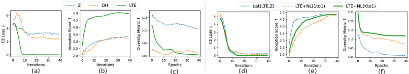
Figure 5: (a-c) Comparing LTE, random noise (Z), and one-hot vector (OH) inputs for the generator. While LTE shows rapid convergence in CE Loss and superior image quality, the diversity metric for LTE and OH are far lower than Z. (d-f) Comparison of using Concatenation of Z and LTE vs. 1-to-1 and K-to-1 noisy layer strategies with LTE input for enhancing generator diversity

Effectiveness of Noisy Layer. We illustrate the impact of utilizing both 1-to-1 and K-to-1 noisy layer strategies in enhancing the generator’s diversity when utilizing LTE as the input. As shown in Fig. 5d-f, shifting the source of randomness from the input to the layer level and reinitializing the noisy layer with each iteration significantly boosts the generator’s diversity while maintaining rapid convergence and high-quality sampling. Moreover, the experiments demonstrate that using a single noisy layer to synthesize a batch of images (K-to-1) results in faster convergence and a higher diversity score when compared to using one noisy layer for each individual image (1-to-1).

Visualization. The synthetic results achieved by NAYER within just 100 generator training steps on ImageNet by employing the ResNet-50 as teacher model are presented in Fig. 6a-b. For further comparison, we also visualize synthetic images generated by NAYER, FM, CMI, and DeepInv in Fig. 6c-f. All of these samples are generated using 20 steps with a ResNet-34 teacher model in the CIFAR-10 dataset. While it remains challenging for human recognition, our method visibly demonstrates superior quality and a more diverse range of images when compared to other methods.

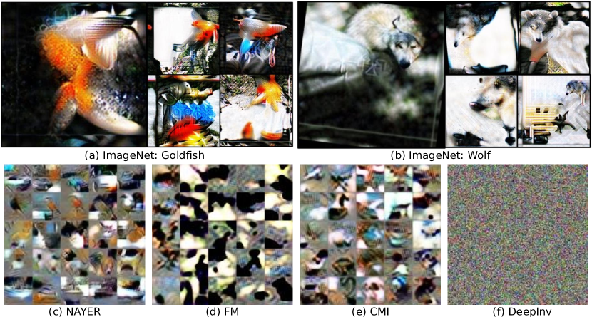
Figure 6: (a, b) Display synthetic data generated by our NAYER for ImageNet in just 100 steps. (c, d, e, f) Showcase synthetic data generated for 5 classes (from top to bottom: Car, Bird, Cat, Dog, Ship) in CIFAR10, using only 20 steps of NAYER, FM, CMI, and DeepInv.

5 Conclusion and Future Works

In this paper, we propose a novel Noisy Layer Generation method (NAYER) which utilizes the meaningful label-text embedding (LTE) as the input and relocates the randomness source from the input to the noisy layer. The significance of LTE lies in its ability to contain substantial meaningful information, enabling the fast generating images in only few steps. On the other hand, the use of noisy layer can help the model address the overfocus problem in using constant input information and increase significantly the diversity. Our extensive experiments on different datasets and tasks prove NAYER’s superiority over other state-of-the-art methods in data-free knowledge distillation.

The proposed NAYER does not incorporate the innovative techniques utilized in current SOTA methods, such as feature mixup (Yu et al., 2023), knowledge acquisition and retention (Patel et al., 2023), and momentum updating (Do et al., 2022). This leaves space for potential improvements through the integration of these techniques in the future. Additionally, NAYER can be applied to various data-free methods, including but not limited to data-free quantization or data-free model stealing.

Appendix A Training Details

A.1 Teacher Model Training Details

In this work, we employed pretrained ResNet-34 and WideResnet-40-2 teacher models from (Fang et al., 2022) for CIFAR-10 and CIFAR-100. For Tiny ImageNet, we trained ResNet-34 from scratch using PyTorch, and for ImageNet, we utilized the pretrained ResNet-50 from PyTorch. Teacher models were trained with SGD optimizer, initial learning rate of 0.1, momentum of 0.9, and weight decay of 5e-4, using a batch size of 128 for 200 epochs. Learning rate decay followed a cosine annealing schedule.

Table 4: Generator Network ($\mathcal{G}$) Architecture for CIFAR10, CIFAR100 and TinyImageNet.

Output Size Layers 1000 Input $128\times h/4\times w/4$ Linear, BatchNorm1D, Reshape $128\times h/4\times w/4$ SpectralNorm (Conv (3 × 3)), BatchNorm2D, LeakyReLU $128\times h/2\times w/2$ UpSample (2×) $64\times h/2\times w/2$ SpectralNorm (Conv (3 × 3)), BatchNorm2D, LeakyReLU $64\times h\times w$ UpSample (2×) $3\times h\times w$ SpectralNorm (Conv (3 × 3)), Sigmoid, BatchNorm2D

Table 5: Generator Network ($\mathcal{G}$) Architecture for ImageNet.

Output Size Layers 1000 Input $128\times h/16\times w/16$ Linear, BatchNorm1D, Reshape $128\times h/16\times w/16$ SpectralNorm (Conv (3 × 3)), BatchNorm2D, LeakyReLU $128\times h/8\times w/8$ UpSample (2×) $128\times h/8\times w/8$ SpectralNorm (Conv (3 × 3)), BatchNorm2D, LeakyReLU $128\times h/4\times w/4$ UpSample (2×) $64\times h/4\times w/4$ SpectralNorm (Conv (3 × 3)), BatchNorm2D, LeakyReLU $64\times h/2\times w/2$ UpSample (2×) $64\times h/2\times w/2$ SpectralNorm (Conv (3 × 3)), BatchNorm2D, LeakyReLU $64\times h\times w$ UpSample (2×) $3\times h\times w$ SpectralNorm (Conv (3 × 3)), Sigmoid, BatchNorm2D

Table 6: The hyperparameters for NAYER applied to four different datasets are detailed below. Specifically, $\alpha_{cls}$, $\alpha_{bn}$, and $\alpha_{adv}$ are the hyperparameters associated with Eq. (2), and their values are consistent with the settings defined in (Fang et al., 2022). The variables $I$ and $S$ denote the number of iterations for generating and training the student, respectively, while $g$ represents the training steps to optimize the generator $\mathcal{G}_{\theta_{\mathcal{G}}}$ and the noisy layers $\mathcal{Z}$.

batch size (student) batch size (generator) $\alpha_{cls}$ $\alpha_{bn}$ $\alpha_{adv}$ $I$ $g$ $S$ CIFAR10 512 400 0.5 10 1.33 2 30 400 CIFAR100 512 400 0.5 10 1.33 2 40 400 TinyImageNet 256 200 0.5 10 1.33 4 60 1000 ImageNet 128 50 0.1 0.1 0.1 20 100 2000

A.2 Student Model Training Details

To ensure fair comparisons, we adopt the generator architecture outlined in (Fang et al., 2022) for all experiments. Specifically, the generator architecture for CIFAR10, CIFAR100, and TinyImageNet is elaborated upon in Table 4, while the generator architecture for ImageNet is provided in Table 5. Across all experiments, we maintain a consistent approach for training the student model, employing a batch size of 512. We utilize the SGD optimizer with a momentum of 0.9 and a variable learning rate, following a cosine annealing schedule that starts at 0.1 and ends at 0, to optimize the student parameters ($\theta_{\mathcal{S}}$). Additionally, we employ the Adam optimizer with a learning rate of 4e-3 for optimizing the generator.We present the results in three distinct variants, each corresponding to a different value of $\mathcal{E}$: 100, 200, and 300, all incorporating a configuration of 20 warm-up epochs, in line with the settings defined in (Fang et al., 2022). Further details regarding the parameters can be found in Table 6.

Appendix B Extended Results

B.1 Comparison with Different Generation Steps

We compare NAYER and FM, both utilizing random noise as input, while adjusting the training steps for their generators. To ensure a level playing field, we use identical generator architectures, including the additional linear layer (noisy layer for NAYER), and train all models for 300 epochs. This approach allows us to assess their performance under consistent conditions and understand how varying the generator training steps impacts their accuracy.

Table 7: The accuracies of our NAYER and FM (which uses random noise as the input) with varying training steps for generators. It’s important to note that for a fair comparison, we employ the same generator architectures, including the additional linear layer (noisy layer for NAYER) for FM. Furthermore, all models are trained for 300 epochs

Generator’s training steps $g=2$ $g=5$ $g=10$ $g=20$ $g=30$ $g=40$ $g=50$ FM 57.08 63.83 65.12 66.82 67.51 68.23 68.18 NAYER 59.23 65.14 68.13 69.31 70.42 71.72 71.70

B.2 Comparison with Different Memory Buffer Size

In this comparison, we evaluate the accuracies of our NAYER (Noisy Label Generator) and MBDFKD models while varying the memory buffer size. It is crucial to highlight that, to ensure a fair and unbiased assessment, we maintain identical generator architectures, including the additional linear layer (noisy layer for NAYER) for both NAYER and MBDFKD. This uniform setup allows us to isolate the impact of memory buffer size on model performance and draw meaningful conclusions about their respective capabilities.

Table 8: The accuracies of our NAYER and MBDFKD models were evaluated while varying the memory buffer size. It’s important to note that for a fair comparison, we employed the same generator architectures, including the additional linear layer (noisy layer for NAYER), for both NAYER and MBDFKD.

Memory buffer size 5k 10k 20k 40k 100k 200k Full MBDFKD 73.33 74.12 73.72 72.68 71.96 71.27 70.72 NAYER 90.41 90.76 90.98 91.21 91.64 91.86 91.94

B.3 Comparison with Different Text Encoder

We analyze the accuracies of our NAYER (Noisy Label Generator) model across three distinct text encoders: Doc2Vec (Le & Mikolov, 2014), SBERT (Reimers & Gurevych, 2019), and CLIP (Radford et al., 2021). This comparative assessment provides valuable insights into how NAYER performs when coupled with different text encoding methodologies.

Table 9: The accuracies of our NAYER with three different text encoders, including Doc2Vec, SBERT, and CLIP.

CIFAR-10 CIFAR-100 Text Encoder Doc2Vec SBERT CLIP Doc2Vec SBERT CLIP Accuracy 93.98 93.94 94.07 71.58 71.63 71.72

B.4 Further Comparison with Different Generation Strategies

In this section, we conduct an extensive comparison of various generation strategies. These strategies encompass using only LTE (LTE), random noise (Z), one-hot vectors (OH), the sum of random noise and one-hot vectors (Do et al., 2022) (sum(OH,Z)), the concatenation of Z and one-hot vectors (Luo et al., 2020; Yoo et al., 2019) (cat(OH,Z)), the concatenation of Z and LTE (cat(LTE,Z)), the sum of Z and LTE (cat(LTE,Z)), utilizing our noisy layer for each LTE (LTE+NL(1to1)), a single noisy layer for all LTE (LTE+NL(1toN)), and the generation methods of DeepInv (Yin et al., 2020) and CMI (Fang et al., 2021). We evaluate these strategies using three metrics: CE Loss to demonstrate convergence speed, IS Score to illustrate image quality, and a diversity metric. It is evident that our proposed method, which leverages the noisy layer for learning LTE, achieves both rapid convergence and high-quality images while maintaining significant diversity.

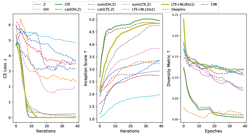
Figure 7: When further comparing various generation strategies based on CE Loss, IS Score, and a diversity metric, it becomes evident that our proposed method, which utilizes the noisy layer for learning LTE, achieves both rapid convergence and high-quality images while maintaining remarkable diversity.

B.5 t-SNE Visuallization of LTE and Ground-truth Dataset Distribution

In this section, we aim to illustrate the interclass information captured by LTE (Label-Text Embedding). To achieve this, we provide t-SNE visualizations of the embeddings for labels and ground-truth data distribution pertaining to four distinct classes: Car, Cat, Dog, and Truck. The t-SNE representation of LTE closely aligns with the ground-truth distribution, especially in the proximity between classes like Car and Truck, as well as Cat and Dog, indicating notably smaller distances compared to other class pairings.

References

- Binici et al. (2022a) Kuluhan Binici, Shivam Aggarwal, Nam Trung Pham, Karianto Leman, and Tulika Mitra. Robust and resource-efficient data-free knowledge distillation by generative pseudo replay. In Proceedings of the AAAI Conference on Artificial Intelligence, volume 36, pp. 6089–6096, 2022a.
- Binici et al. (2022b) Kuluhan Binici, Nam Trung Pham, Tulika Mitra, and Karianto Leman. Preventing catastrophic forgetting and distribution mismatch in knowledge distillation via synthetic data. In Proceedings of the IEEE/CVF winter conference on applications of computer vision, pp. 663–671, 2022b.
- Cai et al. (2020) Yaohui Cai, Zhewei Yao, Zhen Dong, Amir Gholami, Michael W Mahoney, and Kurt Keutzer. Zeroq: A novel zero shot quantization framework. In Proceedings of the IEEE/CVF Conference on Computer Vision and Pattern Recognition, pp. 13169–13178, 2020.
- Choi et al. (2020) Yoojin Choi, Jihwan Choi, Mostafa El-Khamy, and Jungwon Lee. Data-free network quantization with adversarial knowledge distillation. In Proceedings of the IEEE/CVF Conference on Computer Vision and Pattern Recognition Workshops, pp. 710–711, 2020.
- Do et al. (2022) Kien Do, Thai Hung Le, Dung Nguyen, Dang Nguyen, Haripriya Harikumar, Truyen Tran, Santu Rana, and Svetha Venkatesh. Momentum adversarial distillation: Handling large distribution shifts in data-free knowledge distillation. Advances in Neural Information Processing Systems, 35:10055–10067, 2022.
- Fang et al. (2021) Gongfan Fang, Jie Song, Xinchao Wang, Chengchao Shen, Xingen Wang, and Mingli Song. Contrastive model inversion for data-free knowledge distillation. arXiv preprint arXiv:2105.08584, 2021.
- Fang et al. (2022) Gongfan Fang, Kanya Mo, Xinchao Wang, Jie Song, Shitao Bei, Haofei Zhang, and Mingli Song. Up to 100x faster data-free knowledge distillation. In Proceedings of the AAAI Conference on Artificial Intelligence, volume 36, pp. 6597–6604, 2022.
- Frankle & Carbin (2018) Jonathan Frankle and Michael Carbin. The lottery ticket hypothesis: Finding sparse, trainable neural networks. arXiv preprint arXiv:1803.03635, 2018.
- He et al. (2016) Kaiming He, Xiangyu Zhang, Shaoqing Ren, and Jian Sun. Deep residual learning for image recognition. In Proceedings of the IEEE conference on computer vision and pattern recognition, pp. 770–778, 2016.
- Krizhevsky et al. (2009) Alex Krizhevsky, Geoffrey Hinton, et al. Learning multiple layers of features from tiny images. 2009.
- Le & Mikolov (2014) Quoc Le and Tomas Mikolov. Distributed representations of sentences and documents. In International conference on machine learning, pp. 1188–1196. PMLR, 2014.
- Le & Yang (2015) Ya Le and Xuan Yang. Tiny imagenet visual recognition challenge. CS 231N, 7(7):3, 2015.
- Liu et al. (2021) Yuang Liu, Wei Zhang, and Jun Wang. Zero-shot adversarial quantization. In Proceedings of the IEEE/CVF Conference on Computer Vision and Pattern Recognition, pp. 1512–1521, 2021.
- Luo et al. (2020) Liangchen Luo, Mark Sandler, Zi Lin, Andrey Zhmoginov, and Andrew Howard. Large-scale generative data-free distillation. arXiv preprint arXiv:2012.05578, 2020.
- Micaelli & Storkey (2019) Paul Micaelli and Amos J Storkey. Zero-shot knowledge transfer via adversarial belief matching. Advances in Neural Information Processing Systems, 32, 2019.
- Mirza & Osindero (2014) Mehdi Mirza and Simon Osindero. Conditional generative adversarial nets. arXiv preprint arXiv:1411.1784, 2014.
- Nayak et al. (2019) Gaurav Kumar Nayak, Konda Reddy Mopuri, Vaisakh Shaj, Venkatesh Babu Radhakrishnan, and Anirban Chakraborty. Zero-shot knowledge distillation in deep networks. In International Conference on Machine Learning, pp. 4743–4751. PMLR, 2019.
- Patel et al. (2023) Gaurav Patel, Konda Reddy Mopuri, and Qiang Qiu. Learning to retain while acquiring: Combating distribution-shift in adversarial data-free knowledge distillation. In Proceedings of the IEEE/CVF Conference on Computer Vision and Pattern Recognition, pp. 7786–7794, 2023.
- Qiu et al. (2022) Zengyu Qiu, Xinzhu Ma, Kunlin Yang, Chunya Liu, Jun Hou, Shuai Yi, and Wanli Ouyang. Better teacher better student: Dynamic prior knowledge for knowledge distillation. arXiv preprint arXiv:2206.06067, 2022.
- Radford et al. (2021) Alec Radford, Jong Wook Kim, Chris Hallacy, Aditya Ramesh, Gabriel Goh, Sandhini Agarwal, Girish Sastry, Amanda Askell, Pamela Mishkin, Jack Clark, et al. Learning transferable visual models from natural language supervision. In International conference on machine learning, pp. 8748–8763. PMLR, 2021.
- Reimers & Gurevych (2019) Nils Reimers and Iryna Gurevych. Sentence-bert: Sentence embeddings using siamese bert-networks. arXiv preprint arXiv:1908.10084, 2019.
- Salimans et al. (2016) Tim Salimans, Ian Goodfellow, Wojciech Zaremba, Vicki Cheung, Alec Radford, and Xi Chen. Improved techniques for training gans. Advances in neural information processing systems, 29, 2016.
- Sanh et al. (2019) Victor Sanh, Lysandre Debut, Julien Chaumond, and Thomas Wolf. Distilbert, a distilled version of bert: smaller, faster, cheaper and lighter. arXiv preprint arXiv:1910.01108, 2019.
- Simonyan & Zisserman (2014) Karen Simonyan and Andrew Zisserman. Very deep convolutional networks for large-scale image recognition. arXiv preprint arXiv:1409.1556, 2014.
- Yin et al. (2020) Hongxu Yin, Pavlo Molchanov, Jose M Alvarez, Zhizhong Li, Arun Mallya, Derek Hoiem, Niraj K Jha, and Jan Kautz. Dreaming to distill: Data-free knowledge transfer via deepinversion. In Proceedings of the IEEE/CVF Conference on Computer Vision and Pattern Recognition, pp. 8715–8724, 2020.
- Yoo et al. (2019) Jaemin Yoo, Minyong Cho, Taebum Kim, and U Kang. Knowledge extraction with no observable data. Advances in Neural Information Processing Systems, 32, 2019.
- Yoon et al. (2021) Ji Won Yoon, Hyeonseung Lee, Hyung Yong Kim, Won Ik Cho, and Nam Soo Kim. Tutornet: Towards flexible knowledge distillation for end-to-end speech recognition. IEEE/ACM Transactions on Audio, Speech, and Language Processing, 29:1626–1638, 2021.
- Yu et al. (2023) Shikang Yu, Jiachen Chen, Hu Han, and Shuqiang Jiang. Data-free knowledge distillation via feature exchange and activation region constraint. In Proceedings of the IEEE/CVF Conference on Computer Vision and Pattern Recognition, pp. 24266–24275, 2023.
- Zagoruyko & Komodakis (2016) Sergey Zagoruyko and Nikos Komodakis. Wide residual networks. arXiv preprint arXiv:1605.07146, 2016.