Abstract

The dynamical behavior of a scalar field near a rotating loop quantum gravity black hole is investigated. By analyzing the waveform of scalar fields, we find that the loop quantum correction only affects the decaying oscillation of waveforms, which is mainly described by quasi-normal modes. Moreover, we calculate the quasi-normal modes of scalar field perturbations by using three numerical methods, which are the Prony, WKB, and shooting methods, respectively, and compare the accuracy of results among these methods. Over the entire parameter space of a rotating loop quantum gravity black hole, we analyze the stability of the spacetime and the influence of loop quantum corrections on the quasi-normal modes of scalar field perturbations, and find that the influence varies with the change of black hole angular momenta. Finally, we study the energy amplification effect of black holes on free scalar fields, and analyze the influence of loop quantum corrections on the amplification factor. Our result shows the diverse influences of loop quantum corrections on the dynamics of scalar fields and superradiance effect of a rotating loop quantum gravity black hole.

1 Introduction

Although general relativity (GR) is the most widely accepted theory of gravity, it suffers [1, 2] from several challenges and unresolved issues, such as singularity, information loss paradox, and breakdown of predictability, etc. One effective approach to resolve [3] the conundrum of black hole singularities is to construct regular black hole models. In a regular black hole spacetime, there are no intrinsic singularities, thus naturally avoiding the issues associated with intrinsic singularities. Although the first regular black hole was constructed [4] within the scope of GR, many regular black holes have been proposed [5, 6, 7] in the framework of modified gravity theories. Among the various theories, the loop quantum gravity (LQG) aims to construct a unified theory of quantum gravity and address the issue of spacetime singularities. Within the scope of LQG theory, some static and spherically symmetric models of regular black holes have been given [8, 9, 10, 11], where a quantum parameter was introduced to describe the spacetime of regular black holes.

It is known that astrophysical black holes are rotating, which means that the research on static black holes alone has only limited effects on observations. Recently, a rotating model of regular black holes was suggested [12] in the LQG theory, where its shadow was analyzed and connected to possible future observational data [13]. Considering that shadows are only one phenomenon to show the connection between intrinsic properties of black holes and observations, we explore other possible phenomena beyond shadows and investigate their potential observable effects in the scope of LQG theory. In the present work we focus on two phenomena: Quasi-normal modes (QNMs) [14, 15, 16, 17] and superradiance [18, 16, 17].

In GR, the QNM frequencies of scalar field perturbations are determined by the mass of scalar fields, the mass and angular momentum of black holes. QNMs are complex due to the existence of event horizons, so we can divide a QNM frequency into a real part and an imaginary part,

$$\omega=\omega_{\rm R}+i\omega_{\rm I},$$ (1)

where the real part $\omega_{\rm R}$ represents the oscillation frequency and the imaginary part $\omega_{\rm I}$ denotes the decay rate. In previous works [14], it has been noted that QNMs are highly sensitive to boundary conditions, particularly the asymptotic behaviors of scalar fields near event horizons. The difference between a LQG metric and a Kerr metric will lead to differences of boundary conditions and then affect QNMs. In astrophysical observations the ringdown phase after the merger of two black holes is described by perturbation theory and gravitational waves are a linear superposition of QNMs [19, 20, 21]. Through computing the QNMs of scalar field perturbations around a rotating LQG black hole (rLQGBH), we can provide some hints of the underlying gravity theory.

The superradiance effect is a radiation enhancement process in a dissipative system. In black hole theory, the superradiance is closely associated [22, 23, 24, 25] with the ergoregion of rotating black holes. Especially, the superradiance is a powerful tool to detect [18, 26] ultralight scalar fields which are a promising candidate of dark matter. Similarly, the superradiance is also sensitive to boundary conditions, thus the quantum parameter that plays a crucial role in a LQG metric, see Sec. 2 for the details, will leave imprints on the superradiance effects in rLQGBHs, too. We expect to shed some light on the existence of ultralight scalar particles in the LQG theory through the investigation of superradiance.

Our research focuses on QNMs and superradiance effects, both of which need to deal with Klein-Gordon equations with boundary conditions. The difficulty of calculations lies in the complicacy of rLQGBHs, where one aspect comes from the angular equation due to rotations, and the other comes from the complicated radial equation. For example, the Leaver method [27], previously applied to static and spherically symmetric black holes or some simple rotating black holes, is unable to deal with rLQGBHs. Owing to this reason, we employ three other numerical methods, the Prony, WKB, and shooting methods, to calculate the QNMs of scalar field perturbations around rLQGBHs and compare the results among the three methods in order to obtain the most precise QNMs. Moreover, we analyze the superradiance effect in rLQGBHs by adopting the shooting method which is the most efficient one among the three.

The paper is organized as follows. In Sec. 2, we briefly introduce the rotating black holes in loop quantum gravity. In Sec. 3, we analyze the time domain waveform under scalar field perturbations. In Sec. 4, we compute the QNMs of scalar field perturbations around rLQGBHs by using the three numerical methods. In Sec. 5, we apply the shooting method to calculate the amplification factor. Finally, we give our conclusion in Sec. 6. The natural units $(G=c=\hbar=1)$ are adopted in our paper.

2 Rotating black holes in loop quantum gravity

In this section we briefly describe the geometry of rLQGBHs. From a static and spherically symmetric LQGBH, its rotating counterpart was constructed [12, 28] in terms of the modified Newman-Janis algorithm. In the Boyer-Lindquist coordinates $(t,r,\theta,\varphi)$, the line element of rLQGBHs reads

$${\mathrm{d}}s^{2}=-\left(1-\frac{2Mb}{\rho^{2}}\right){\mathrm{d}}t^{2}-\frac{4aMb\mathrm{sin}^{2}\theta}{\rho^{2}}{\mathrm{d}}t{\mathrm{d}}\varphi+\rho^{2}{\mathrm{d}}\theta^{2}+\frac{\rho^{2}}{\Delta}{\mathrm{d}}r^{2}+\frac{\Sigma\mathrm{sin}^{2}\theta}{\rho^{2}}{\mathrm{d}}\varphi^{2},$$ (2)

where

$$\rho^{2} = a^{2}\mathrm{cos}^{2}\theta+b^{2},$$ (3)

$$\Delta = b^{2}+a^{2}-2Mb,$$ (4)

$$\Sigma = \left(b^{2}+a^{2}\right)^{2}-a^{2}\Delta\mathrm{sin}^{2}\theta,$$ (5)

$$b^{2} = \frac{A_{\lambda}}{\sqrt{1+x^{2}}}\frac{M_{\rm B}^{2}\left(x+\sqrt{1+x^{2}}\right)^{6}+M_{\rm B}^{2}}{\left(x+\sqrt{1+x^{2}}\right)^{3}},$$ (6)

$$M = \frac{b}{2}\left[1-\frac{8A_{\lambda}M_{\rm B}^{2}}{b^{2}}\left(1-\sqrt{\frac{1}{2A_{\lambda}}}\frac{1}{\sqrt{1+x^{2}}}\right)\left(1+x^{2}\right)\right],$$ (7)

$$x = \frac{r}{\sqrt{8A_{\lambda}}M_{\rm B}}.$$ (8)

Here the angular momentum $a$ and Arnowitt-Deser-Misner (ADM) mass $M_{\rm B}$ are assumed to be positive, and $A_{\lambda}$ is a positive dimensionless quantum parameter originated [10] from holonomy modifications. The above rLQGBH is regular [12] everywhere when $A_{\lambda}>0$ and reduces to a Kerr black hole when $A_{\lambda}=0$. By introducing the transformation,

$$h=\sqrt{r^{2}+8A_{\lambda}M_{\rm B}^{2}},$$ (9)

we simplify $b^{2}$, $M$, and $\Delta$ to be

$$b^{2} = h^{2}-6A_{\lambda}M_{\rm B}^{2},$$ (10)

$$Mb = M_{\rm B}h-3A_{\lambda}M_{\rm B}^{2}.$$ (11)

$$\Delta = h^{2}+a^{2}-2M_{\rm B}h,$$ (12)

The location of horizons can be determined by the algebraic equation,

$$\Delta=h^{2}+a^{2}-2M_{\rm B}h=0,$$ (13)

and its solutions are

$$h_{\pm}=M_{\rm B}\pm\sqrt{M_{\rm B}^{2}-a^{2}},$$ (14)

where a plus or minus sign represents an outer or inner horizon. According to the existence of an outer horizon, we restrict the two dimensionless parameters, $A_{\lambda}$ and $a/M_{\rm B}$ in the shadow region of Fig. 1, where the blue curve corresponds to the extreme configuration. From the parameter space $(A_{\lambda},a/M_{\rm B})$, we obtain that the maximum value of angular momenta equals one, $a_{\rm Max}/{M_{\rm B}}=1$, which will be adopted in the numerical calculations below. For a given angular momentum $a$, the entire range of quantum parameter $A_{\lambda}$ is $0\leq A_{\lambda}\leq A_{\lambda\mathrm{Max}}$, where the extreme configuration of rLQGBHs takes the maximum value of quantum parameter $A_{\lambda}$,

$$A_{\lambda\mathrm{Max}}=\frac{1}{8}\left(1+\sqrt{1-\frac{a^{2}}{M_{\rm B}^{2}}}\right)^{2}.$$ (15)

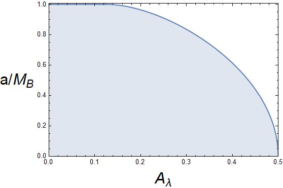
Figure 1: The parameter space $(A_{\lambda},a/M_{\rm B})$ of rLQGBH spacetime, where the shadow region is allowed.

3 Time domain waveform

The evolution of perturbations can be divided [14] into three distinct stages. At first, the perturbation field undergoes an initial outburst, and then a relatively long period of decaying oscillation, and finally an exponential late-time tail. In this section we focus on the impact of quantum parameter $A_{\lambda}$ on the whole time domain evolution of scalar fields.

3.1 Numerical method

When a massive scalar field $\Phi$ acts as perturbation around an rLQGBH, its equation of motion is the Klein-Gordon equation,

$$\nabla^{\nu}\nabla_{\nu}\Phi=\mu^{2}\Phi,$$ (16)

where $\mu$ is the mass of scalar fields. In this section we merely consider massless scalar fileds, so we set $\mu=0$. Generally, we can simulate the waveform $\Phi$ of scalar fields by solving the above equation in $(t,r,\theta,\varphi)$ coordinates. However, the traditional (2+1)-dimensional simulations around rotating black holes often suffer [29, 30] from a serious boundary problem because of the Cauchy foliation, which destroys the precision of numerical calculations. To address this issue, we employ the hyperbolic foliation-dependent strategy [31, 32, 33, 34, 35, 36, 37, 38] to compute the evolution waveform in time domain in order to avoid the subtle boundary problem through the following two coordinate transformations.

In the first transformation, we construct the horizon-penetrating coordinates $\{\tilde{t},h,\theta,\tilde{\varphi}\}$ through

$$\mathrm{d}\tilde{t}=\mathrm{d}t+\frac{2Mb}{\epsilon\Delta}\mathrm{d}h,\qquad\mathrm{d}\tilde{\varphi}=\mathrm{d}\varphi+\frac{a}{\epsilon\Delta}\mathrm{d}h,$$ (17)

where

$$\epsilon=\sqrt{1-\frac{8A_{\lambda}M_{\rm B}^{2}}{h^{2}}}.$$ (18)

The rLQGBH metric Eq. (2) then becomes

$$\begin{split}\mathrm{d}s^{2}=&-\left(1-\frac{2Mb}{\rho^{2}}\right)\mathrm{d}\tilde{t}^{2}-\frac{4aMb}{\rho^{2}}\mathrm{sin}^{2}\theta\mathrm{d}\tilde{t}\mathrm{d}\tilde{\varphi}+\frac{4Mb}{\epsilon\rho^{2}}\mathrm{d}\tilde{t}\mathrm{d}h\\ &+\frac{1}{\epsilon^{2}}\left(1+\frac{2Mb}{\rho^{2}}\right)\mathrm{d}h^{2}-\frac{2}{\epsilon}a\mathrm{sin}^{2}\theta\left(1+\frac{2Mb}{\rho^{2}}\right)\mathrm{d}h\mathrm{d}\tilde{\varphi}\\ &+\rho^{2}\mathrm{d}\theta^{2}+\left(b^{2}+a^{2}+\frac{2Mba^{2}\mathrm{sin}^{2}\theta}{\rho^{2}}\right)\mathrm{sin}^{2}\theta\mathrm{d}\tilde{\varphi}^{2}.\end{split}$$ (19)

Since the metric does not contain $\tilde{\varphi}$ explicitly, $\partial_{\tilde{\varphi}}$ is Killing vector. In order to preserve this feature under the time domain evolution, we only separate variable $\tilde{\varphi}$ in the waveform of scalar field perturbations,

$$\Phi(\tilde{t},h,\theta,\tilde{\phi})=\frac{1}{h}\sum_{m}\psi(\tilde{t},h,\theta)\mathrm{e}^{im\tilde{\varphi}},$$ (20)

where $m$ is azimuthal number. After substituting the above expression into Eq. (16) and considering a massless scalar field, we express the Klein-Gordon equation as

$$A^{\tilde{t}\tilde{t}}\partial^{2}_{\tilde{t}}\psi+A^{\tilde{t}h}\partial_{\tilde{t}}\partial_{h}\psi+A^{hh}\partial^{2}_{h}\psi+A^{\theta\theta}\partial^{2}_{\theta}\psi+B^{\tilde{t}}\partial_{\tilde{t}}\psi+B^{h}\partial_{h}\psi+B^{\theta}\partial_{\theta}\psi+C\psi=0,$$ (21)

where

$$A^{\tilde{t}\tilde{t}} = \rho^{2}+2Mb,$$

$$A^{\tilde{t}h} = -4\epsilon Mb,$$

$$A^{hh} = -\epsilon^{2}\Delta,$$

$$A^{\theta\theta} = -1,$$

$$B^{\tilde{t}} = 2M_{B}\epsilon-\epsilon\frac{12A_{\lambda}M_{B}^{2}}{h},$$

$$B^{h} = \epsilon^{2}\frac{2}{h}(a^{2}-M_{B}h)-2ima\epsilon-\epsilon\Delta\frac{\mathrm{d}}{\mathrm{d}h}\epsilon,$$

$$B^{\theta} = -\mathrm{cot}\theta,$$

$$C = \frac{m^{2}}{\mathrm{sin}^{2}\theta}-\epsilon^{2}\frac{2(a^{2}-M_{B}h)}{h^{2}}+\epsilon\frac{2ima}{h}+\epsilon\frac{\Delta}{h}\frac{\mathrm{d}}{\mathrm{d}h}\epsilon.$$ (22)

In the second transformation, we introduce the hyperbolic foliation [39] to define the compact horizon-penetrating and hyperboloidal coordinates (HH coordinates), $\{\tau,\tilde{r},\theta,\tilde{\varphi}\}$,

$$\tilde{t}=\tau+f(\tilde{r}),\qquad h=\frac{\tilde{r}}{\Omega(\tilde{r})},$$ (23)

where

$$f(\tilde{r})=\frac{\tilde{r}}{\Omega({\tilde{r}})}-{\tilde{r}}-4M_{\rm B}\,\mathrm{ln}\,\Omega({\tilde{r}}),\qquad\Omega({\tilde{r}})=1-\frac{\tilde{r}}{S}.$$ (24)

Here $S$ is a constant associated with the hyperbolic foliation. According to this coordinate transformation and Eq. (14), we obtain the location of outer horizon,

$${\tilde{r}}_{+}=\frac{a^{2}S+\left(M_{\rm B}+\sqrt{M_{\rm B}^{2}-a^{2}}\right)S^{2}}{a^{2}+2M_{\rm B}S+S^{2}},$$ (25)

and the relations between the HH coordinates and the horizon-penetrating coordinates,

$$\partial_{\tilde{t}}=\partial_{\tau},\qquad\partial_{h}=-H\partial_{\tau}+K\partial_{\tilde{r}},$$ (26)

where

$$H=\frac{\mathrm{d}f}{\mathrm{d}h}({\tilde{r}}),\qquad K=\frac{\mathrm{d}{\tilde{r}}}{\mathrm{d}h}({\tilde{r}}).$$ (27)

Therefore, the Klein-Gordon equation Eq. (21) can be expressed in the HH coordinate as follows:

$$\partial^{2}_{\tau}\psi={\tilde{A}}^{\tau{\tilde{r}}}\partial_{\tau}\partial_{\tilde{r}}\psi+{\tilde{A}}^{{\tilde{r}}{\tilde{r}}}\partial^{2}_{\tilde{r}}\psi+{\tilde{A}}^{\theta\theta}\partial^{2}_{\theta}\psi+{\tilde{B}}^{\tau}\partial_{\tau}\psi+{\tilde{B}}^{\tilde{r}}\partial_{\tilde{r}}\psi+{\tilde{B}}^{\theta}\partial_{\theta}\psi+{\tilde{C}}\psi,$$ (28)

where

$$\{{\tilde{A}}^{\tau{\tilde{r}}},{\tilde{A}}^{{\tilde{r}}{\tilde{r}}},{\tilde{A}}^{\theta\theta},{\tilde{B}}^{\tau},{\tilde{B}}^{\tilde{r}},{\tilde{B}}^{\theta},{\tilde{C}}\} = -\frac{1}{A^{\tau\tau}}\{{A}^{\tau{\tilde{r}}},{A}^{{\tilde{r}}{\tilde{r}}},{A}^{\theta\theta},{B}^{\tau},{B}^{\tilde{r}},{B}^{\theta},{C}\},$$

$$A^{\tau\tau} = A^{\tilde{t}\tilde{t}}-HA^{\tilde{t}h}+H^{2}A^{hh},$$

$$A^{\tau{\tilde{r}}} = KA^{\tilde{t}h}-2KHA^{hh},$$

$$A^{{\tilde{r}}{\tilde{r}}} = K^{2}A^{hh},$$

$$B^{\tau} = B^{\tilde{t}}-HB^{h}-\frac{\mathrm{d}H}{\mathrm{d}{\tilde{r}}}KA^{hh},$$

$$B^{\tilde{r}} = K\left(B^{h}+\frac{\mathrm{d}K}{\mathrm{d}{\tilde{r}}}A^{hh}\right).$$ (29)

In order to numerically solve Eq. (28) , we introduce an auxiliary function $\Pi$, so that we can reduce this equation to two first-order equations,

$$\partial_{\tau}\psi = \Pi,$$ (30)

$$\partial_{\tau}\Pi = {\tilde{B}}^{\tau}\Pi+{\tilde{A}}^{\tau{\tilde{r}}}\partial_{\tilde{r}}\Pi+{\tilde{A}}^{{\tilde{r}}{\tilde{r}}}\partial^{2}_{\tilde{r}}\psi+{\tilde{A}}^{\theta\theta}\partial^{2}_{\theta}\psi+{\tilde{B}}^{\tilde{r}}\partial_{\tilde{r}}\psi+{\tilde{B}}^{\theta}\partial_{\theta}\psi+{\tilde{C}}\psi,$$ (31)

which can be solved by the fourth-order Runge-Kutta method. Here we take a Gaussian distribution as the initial condition,

$$\psi(\tau=0,{\tilde{r}},\theta) = Y_{lm}\,{\exp}\left[-\frac{({\tilde{r}}-{\tilde{r}}_{c})^{2}}{2\sigma^{2}}\right],$$

$$\Pi(\tau=0,{\tilde{r}},\theta) = 0,$$ (32)

where $Y_{lm}$ is the $\theta$-dependent part of spherical harmonics, and $\tilde{r}_{c}$ and $\sigma$ are the center and the width of Gaussian packets, respectively. When we choose the location of our observer $\tilde{r}_{c}=6M_{\rm B}$, $\theta=\frac{\pi}{4}$, the width $\sigma=0.2$, and the free parameter $S=10$ as suggested by Refs. [39, 30], we solve Eqs. (30) and (31) and obtain the time domain evolution profiles as shown in Fig. 2.

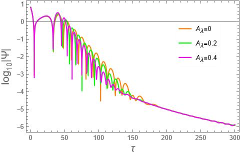
Figure 2: The waveform of massless scalar field perturbations with a varying $A_{\lambda}$, where the initial mode is chosen to be $l=1=m$, and $M_{\rm B}=1$ and $a=0.1$ are set.

3.2 Results

As an exploratory attempt we choose $l=1=m$ as our initial mode and draw the waveform of a massless scalar field perturbation around an rLQGBH in Fig. 2. Analyzing the evolution profiles, we observe that the introduction of quantum parameter $A_{\lambda}$ does not significantly affect the evolution of outbursts and late-time tails. However, it exerts a notable influence on the damping oscillation phase, that is, an increase of $A_{\lambda}$ leads to an accelerated oscillation and a rapider decay of scalar fields. Therefore, in order to distinguish LQG from GR, i.e., an rLQGBH from a Kerr black hole, we need to study the QNM frequencies of the damping oscillation stage. In the subsequent section, we provide a detailed investigation on the influence of $A_{\lambda}$ on the QNMs under scalar field perturbations.

4 Quasi-normal modes

If a scalar field meets the specific boundary conditions: Pure ingoing waves exist at the outer horizon, while pure outgoing waves exist at the spatial infinity, the characteristic complex frequencies of damping oscillations are just QNMs. Owing to the complicated boundary conditions around rLQGBHs, it is not feasible to obtain QNMs precisely through analytical methods. As a result, various numerical and semi-analytical methods have been adopted [14, 15, 16, 40, 41, 42, 17, 43, 44]. Each method possesses its own advantages and disadvantages, so that the accuracy of results cannot be guaranteed if one relies solely on a single method. In this section, we employ three methods to compute QNMs and make comparisons among them in order to ensure the accuracy and reliability of our findings.

4.1 Prony method

In Sec. 3 we have presented the approach for obtaining time domain profiles of massless scalar field perturbations in rLQGBHs. Now we can extract QNMs from these profiles by the Prony method [14, 40]. The main idea of this method is to fit the profile data with a superposition of damped exponents,

$$\Phi(t)\sim\sum_{j=1}^{p}C_{j}e^{-i\omega_{j}t},$$ (33)

where $C_{j}$ is the amplitude coefficient of QNMs. In computations, we extract $(2p-1)$ equidistant points from the ringdown phase of a profile. These points are used to form one $p\times p$ matrix in order to calculate $\omega_{j}$. Here rows and columns of this matrix are composed of equidistant points with decreasing sequence numbers. Among the $p$ $\omega_{j}^{\prime}s$, the one with the largest $|C_{j}|$ is dominant, which is our demanding QNM frequency. Nevertheless, the Prony method has two sides: Advantage and disadvantage. The former is its high precision [30], while the latter is its non-suitability for massive scalar fields. Therefore, we have to ask for alternative methods to compute the QNMs of massive scalar field perturbations in the following sections.

4.2 WKB method

The WKB method is a semi-analytic technique for determining low-lying QNMs [44]. Assuming that a scalar field has the same symmetry as that of its background spacetime, we can make the following ansatz,

$$\Phi(t,h,\theta,\varphi)=\int{e^{-i\omega t}\sum_{l,m}S_{lm}(\theta)R_{lm}(h)e^{im\varphi}}\mathrm{d}\omega,$$ (34)

where $h$ is defined by Eq. (9) and $\omega$ denotes the characteristic frequency of scalar fields. After separating variables, we obtain the angular equation,

$$\frac{1}{\mathrm{sin}\theta}\frac{\mathrm{d}}{{\mathrm{d}}\theta}\left[\mathrm{sin}\theta\frac{\mathrm{d}}{{\mathrm{d}}\theta}S_{lm}(\theta)\right]+\left[a^{2}\left(\omega^{2}-\mu^{2}\right)\mathrm{cos}^{2}\theta-\frac{m^{2}}{\mathrm{sin}^{2}\theta}+A_{lm}\right]S_{lm}(\theta)=0,$$ (35)

where $S_{lm}(\theta)$’s are spherical harmonics [17], which reduce to $Y_{lm}$’s when $a^{2}(\omega^{2}-\mu^{2})\cos^{2}\theta=0$, and $A_{lm}$ is angular eigenvalue, and also derive the radial equation,

$$\epsilon\frac{\mathrm{d}}{{\mathrm{d}}h}\left[\epsilon\Delta\frac{\mathrm{d}}{{\mathrm{d}}h}R_{lm}(h)\right]+\left[\frac{\tilde{K}^{2}}{\Delta}-\mu^{2}b^{2}-(A_{lm}-2am\omega+a^{2}\omega^{2})\right]R_{lm}(h)=0,$$ (36)

where $\tilde{K}=am-(b^{2}+a^{2})\omega$. If we introduce the following transformation,

$$\Psi(y)=(b^{2}+a^{2})^{1/2}R_{lm}(h),$$ (37)

we can change the radial equation of motion to a Schrödinger-like one,

$$\frac{\mathrm{d}^{2}}{{\mathrm{d}}y^{2}}\Psi(y)+\left[\omega^{2}-V(y)\right]\Psi(y)=0,$$ (38)

where $y$ is the tortoise coordinate determined by

$$\frac{\mathrm{d}h}{{\mathrm{d}}y}=\frac{\epsilon\Delta}{b^{2}+a^{2}},$$ (39)

and $V(y)$ is the effective potential,

$$V(y) = V_{1}+V_{2},$$

$$V_{1} = \frac{\Delta}{h(b^{2}+a^{2})^{4}}\Big{\{}-96A_{\lambda}^{2}M_{\rm B}^{4}(M_{\rm B}-h)+a^{4}h+2M_{\rm B}h^{4}$$

$$-2A_{\lambda}M_{\rm B}^{2}h^{2}(4M_{\rm B}+5h)+a^{2}\left[h^{2}(-4M_{\rm B}+h)+2A_{\lambda}M_{\rm B}^{2}(8M_{\rm B}+h)\right]\Big{\}},$$

$$V_{2} = \frac{\Delta}{(b^{2}+a^{2})^{2}}\left[\frac{\tilde{K}^{2}}{\Delta}-\mu^{2}b^{2}-(A_{lm}-2am\omega+a^{2}\omega^{2})\right].$$ (40)

Following Refs. [17, 45] we choose the fourth-order WKB approximation to numerically solve the radial equation because its relative error is very small. The QNM frequency $\omega$ can be obtained by the WKB formula [43, 46],

$$\frac{i\left[\omega^{2}-V(y_{0})\right]}{\sqrt{-2V^{\prime\prime}(y_{0})}}-\sum_{j=2}^{4}\Lambda_{j}=n+\frac{1}{2},\qquad n=0,1,2,\cdots,$$ (41)

where the prime means the derivative with respect to the tortoise coordinate, $y_{0}$ is fixed by the condition,

$$\frac{\mathrm{d}}{\mathrm{d}y}V(y)\Big{|}_{y=y_{0}}=0,$$ (42)

and $\Lambda_{j}$ denotes higher (than one) order corrections dependent on $V(y_{0})$ and its higher order derivatives.

A rotating black hole is more complicated than a static one because both the scalar potential $V(y)$ and the angular eigenvalue $A_{lm}$ depend on frequency $\omega$ in the former case. For massless scalar field perturbations, we adopt the series expansion method [44] to solve Eq. (41) up to the order of $(a\omega)^{6}$. However, for massive scalar field perturbations, the angular eigenvalue $A_{lm}$ should be expanded [47] as a series of $(a\sqrt{\omega^{2}-\mu^{2}})$, where it contains only even-order terms,

$$A_{lm}=\sideset{{}_{0}}{{}^{lm}_{0}}{\mathop{f}}+\sideset{{}_{0}}{{}^{lm}_{2}}{\mathop{f}}a^{2}(\omega^{2}-\mu^{2})+\sideset{{}_{0}}{{}^{lm}_{4}}{\mathop{f}}a^{4}(\omega^{2}-\mu^{2})^{2}+\cdots,$$ (43)

and $\sideset{{}_{0}}{{}^{lm}_{j}}{\mathop{f}}$ is the $j$th order expansion coefficient. By employing the expressions of $A_{lm}$ and $y_{0}$, we can also express both $V_{0}$ and its higher order derivatives as series of $(a\omega)$ up to order $(a\omega)^{6}$. Finally, we solve Eq. (41) numerically and determine the QNMs with given $a$, $\mu$, $n$, $l$, and $m$.

The advantage of the WKB method lies in its polynomial formula with which we can obtain QNMs with high accuracy through simple numerical calculations. As discussed above, this method depends only on the first six terms of series expansions. However, these terms diverge in certain cases, which leads to a breakdown of the method. When we apply the WKB method in rLQGBHs, we shall discuss its scope of applicability in Sec. 4.4.

4.3 Shooting method

The shooting method is a numerical technique [41, 17] for the calculation of QNMs in black hole physics. Its main idea lies in numerically integrating radial equation of motion from one point near an event horizon to an intermediate point and also from the other point near the spatial infinity to this intermediate point, and then we require that both the wave functions and their first derivatives obtained from the two sides are equal at the intermediate point.

To achieve the goal, we analyze the asymptotic behaviors of the radial equation, Eq. (36). The outer event horizon $h=h_{+}$ and spatial infinity $h=h_{\infty}$ are two regular singularities, thus we can give the radial wave function $R(h)$ by two series that are convergent in the range of $h_{+}<h<h_{\infty}$. Near the outer horizon, the asymptotic formulation of radial wave function $R(h)$ reads

$$R(h)\sim(h-h_{+})^{\pm i\alpha},$$ (44)

where

$$\alpha=\frac{am-2M_{\rm B}\omega(h_{+}-3A_{\lambda}M_{\rm B})}{\epsilon_{+}(h_{+}-h_{-})},\qquad\epsilon_{+}=\sqrt{1-\frac{8A_{\lambda}M_{\rm B}^{2}}{h_{+}^{2}}},$$ (45)

$h_{+}$ and $h_{-}$ are determined by Eq. (14) for rLQGBHs. Near the spatial infinity, it takes the form,

$$R(h)\sim\frac{1}{h}\mathrm{e}^{\pm qh}h^{\pm M_{\rm B}(\mu^{2}-2\omega^{2})/q},$$ (46)

where

$$q=\sqrt{\mu^{2}-\omega^{2}}.$$ (47)

In Eq. (44) the plus and minus signs correspond to ingoing and outgoing waves, respectively. In contrast, the plus and minus signs correspond to outgoing and ingoing waves in Eq. (46), respectively.

The QNMs are eigenvalues of wave equations satisfying specific boundary conditions, where only ingoing waves exist near event horizons and only outgoing waves at the spatial infinity. Therefore, we determine the asymptotic formulations of radial wave functions,

$$R(h)\sim(h-h_{+})^{i\alpha},$$ (48)

and

$$R(h)\sim\frac{1}{h}\mathrm{e}^{qh}h^{M_{\rm B}(\mu^{2}-2\omega^{2})/q},$$ (49)

near the outer horizon and near the spatial infinity, respectively.

Now we can determine the QNMs with the shooting method in the range of $h_{+}<h<h_{\infty}$. In the first step, we choose a QNM frequency as our initial value, with which we can determine the angular eigenvalue $A_{lm}$ by using the Leaver method [27]. In the second step, considering the asymptotic behavior Eq. (48) near the outer horizon, we integrate Eq. (36) from the outer event horizon to an intermediate point, where this point is usually chosen with the maximum value of the potential. In the third step, considering the asymptotic behavior Eq. (49) near the infinity, we integrate Eq. (36) from the infinity to this intermediate point. In the final step, we require that the radial wave function $R(h)$ and its first derivative $R^{\prime}(h)$ are continuous at the intermediate point and thus obtain a QNM frequency. Regarding this QNM frequency as the initial value for the next calculation, i.e. after an iterative process we at last get a stable QNM frequency.

The shooting method is very stable so that it can handle some situations in which the WKB method fails. However, it is not easy in the shooting method to give an initial value of QNMs and to make sure that it does not deviate from the expected value of QNMs too large. Otherwise, the shooting method does not work well. In practical applications, the first initial value will be fixed with the help of other numerical methods, and then the result from the previous iteration is regarded as the initial value for the next iteration.

4.4 Numerical results

4.4.1 Comparison of accuracy among three methods

With the above three methods, we are able to obtain the QNMs of scalar field perturbations around rLQGBHs. Here we start by presenting the QNMs of massless scalar field perturbations with a varying $A_{\lambda}$ in Tab. 1, where two modes with $l=1=m$ and $l=2=m$ are chosen. In the special case of $A_{\lambda}=0$, an rLQGBH reduces to a Kerr black hole, and our results are consistent with those computed by the Leaver method [48].

Since the Prony method is completely a numerical calculation of waveform simulations, its accuracy and reliability are the highest among the three methods, so we take its results as the standard to measure the accuracy of the results from the other two methods. Here, we define the relative error between data $D$ and standard data $SD$ as follows:

$${\rm Err}=\left|\frac{D-SD}{D}\right|,$$ (50)

and display the relative errors between the QNMs obtained by the Prony method and those by the other two methods in brackets of Tab. 1, where the left shows the relative error of real parts, while the right that of imaginary parts. We can see that the relative errors are always less than $2\%$, indicating that both the WKB method and shooting method exhibit high accuracy within the range of quantum parameter, $0\leq A_{\lambda}\leq 0.45$. However, in the mode of $l=1=m$, the relative errors associated with the WKB method grow with an increase of quantum parameter $A_{\lambda}$, which implies that this method may not work well when other parameters, such as angular momenta, take a certain range.

In order to further study the scope of application of the WKB method and the impact of angular momentum $a$ on the QNMs of massless (massive) scalar field perturbations, we display in Tab. 2 the relationship between the QNMs and $a$, where $A_{\lambda}=0.1$ and $l=1=m$ are set. When $a\lesssim 0.4$, the QNMs obtained from the three (two) methods are consistent. However, when $a\gtrsim 0.4$, the discrepancy between the WKB method and the other two methods (shooting method) rapidly increases. The reason is that the series of $(a\omega)$ no longer converges in the WKB method if $a\gtrsim 0.4$, rendering the WKB method inapplicable. On the other hand, as shown in Tab. 1, the shooting method yields less relative errors than the 4th-order WKB, showing that the former exhibits higher precision than the latter. Again considering the shooting method is much more efficient than the Prony method because the latter relies on complicated waveform simulations, we therefore prefer to apply the shooting method to the calculation of amplification factors in Sec. 5.

$l=1=m$
$A_{\lambda}$	Prony method	4th-order WKB	Shooting method
0	$0.3010-0.0975i$	$0.3011-0.0973i(0.03\%,0.20\%)$	$0.3010-0.0973i(0.00\%,0.20\%)$
0.05	$0.3119-0.0998i$	$0.3119-0.0996i(0.00\%,0.20\%)$	$0.3118-0.0996i(0.03\%,0.20\%)$
0.10	$0.3242-0.1023i$	$0.3242-0.1022i(0.00\%,0.10\%)$	$0.3240-0.1023i(0.06\%,0.00\%)$
0.15	$0.3382-0.1050i$	$0.3382-0.1049i(0.00\%,0.10\%)$	$0.3381-0.1053i(0.03\%,0.29\%)$
0.20	$0.3544-0.1080i$	$0.3545-0.1077i(0.03\%,0.28\%)$	$0.3546-0.1082i(0.06\%,0.18\%)$
0.25	$0.3735-0.1114i$	$0.3738-0.1108i(0.08\%,0.54\%)$	$0.3738-0.1112i(0.08\%,0.18\%)$
0.30	$0.3964-0.1150i$	$0.3968-0.1140i(0.10\%,0.87\%)$	$0.3962-0.1147i(0.05\%,0.26\%)$
0.35	$0.4245-0.1190i$	$0.4252-0.1174i(0.16\%,1.34\%)$	$0.4243-0.1193i(0.05\%,0.25\%)$
0.40	$0.4604-0.1229i$	$0.4612-0.1207i(0.17\%,1.79\%)$	$0.4608-0.1227i(0.09\%,0.16\%)$
0.45	$0.5082-0.1256i$	$0.5093-0.1232i(0.22\%,1.91\%)$	$0.5079-0.1258i(0.06\%,0.16\%)$

$l=2=m$
$A_{\lambda}$	Prony method	4th-order WKB	Shooting method
0	$0.4995-0.0967i$	$0.4995-0.0966i(0.00\%,0.10\%)$	$0.4994-0.0967i(0.02\%,0.00\%)$
0.05	$0.5179-0.0989i$	$0.5179-0.0989i(0.00\%,0.00\%)$	$0.5180-0.0990i(0.02\%,0.10\%)$
0.10	$0.5388-0.1015i$	$0.5388-0.1014i(0.00\%,0.10\%)$	$0.5389-0.1014i(0.02\%,0.10\%)$
0.15	$0.5627-0.1042i$	$0.5627-0.1042i(0.00\%,0.00\%)$	$0.5626-0.1042i(0.02\%,0.00\%)$
0.20	$0.5904-0.1073i$	$0.5904-0.1073i(0.00\%,0.00\%)$	$0.5903-0.1074i(0.02\%,0.09\%)$
0.25	$0.6231-0.1108i$	$0.6231-0.1107i(0.00\%,0.09\%)$	$0.6232-0.1107i(0.02\%,0.09\%)$
0.30	$0.6626-0.1146i$	$0.6626-0.1145i(0.00\%,0.09\%)$	$0.6624-0.1146i(0.03\%,0.00\%)$
0.35	$0.7114-0.1187i$	$0.7115-0.1185i(0.01\%,0.17\%)$	$0.7116-0.1187i(0.03\%,0.00\%)$
0.40	$0.7743-0.1229i$	$0.7743-0.1225i(0.00\%,0.32\%)$	$0.7743-0.1229i(0.00\%,0.00\%)$
0.45	$0.8588-0.1255i$	$0.8587-0.1250i(0.01\%,0.40\%)$	$0.8588-0.1257i(0.00\%,0.16\%)$

Table 1: QNMs for the modes of $l=1=m$ and $l=2=m$, respectively, where $a=0.1$, $M_{\rm B}=1$, and $\mu=0$ are set.

	$\mu=0$			$\mu=0.1$
$a$	Prony method	4th-order WKB	Shooting method	4th-order WKB	Shooting method
0	$0.3145-0.1024i$	$0.3146-0.1022i$	$0.3144-0.1022i$	$0.3187-0.0998i$	$0.3186-0.0996i$
0.1	$0.3242-0.1023i$	$0.3242-0.1022i$	$0.3240-0.1023i$	$0.3281-0.0999i$	$0.3278-0.0999i$
0.2	$0.3351-0.1020i$	$0.3351-0.1019i$	$0.3349-0.1022i$	$0.3388-0.0998i$	$0.3385-0.1000i$
0.3	$0.3474-0.1014i$	$0.3474-0.1012i$	$0.3475-0.1016i$	$0.3509-0.0993i$	$0.3509-0.0998i$
0.4	$0.3617-0.1004i$	$0.3617-0.0995i$	$0.3619-0.1004i$	$0.3649-0.0978i$	$0.3651-0.0989i$
0.5	$0.3785-0.0987i$	$0.3782-0.0939i$	$0.3785-0.0986i$	$0.3808-0.0923i$	$0.3816-0.0972i$
0.6	$0.3987-0.0962i$	$0.3909-0.0761i$	$0.3986-0.0961i$	$0.3924-0.0752i$	$0.4013-0.0949i$
0.7	$0.4242-0.0921i$	$0.3849-0.0530i$	$0.4242-0.0921i$	$0.3860-0.0530i$	$0.4265-0.0912i$
0.8	$0.4585-0.0850i$	$0.3693-0.0380i$	$0.4585-0.0849i$	$0.3697-0.0381i$	$0.4605-0.0843i$
0.9	$0.5116-0.0706i$	$0.3535-0.0292i$	$0.5116-0.0706i$	$0.3529-0.0292i$	$0.5129-0.0703i$

Table 2: QNMs for the mode of $l=1=m$ with $A_{\lambda}=0.1$, $a=0.1$, $M_{\rm B}=1$, $\mu=0$ or $\mu=0.1$. Note that the Prony method is unsuitable for massive scalar field perturbations.

4.4.2 Data of quasi-normal modes

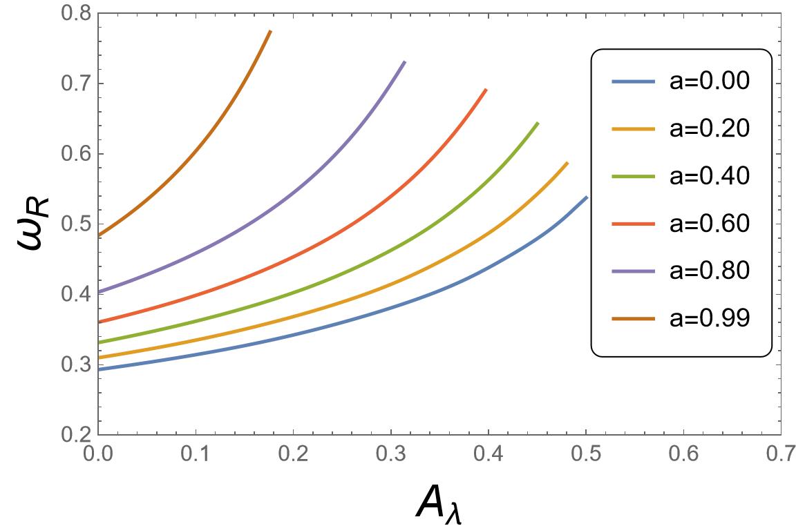
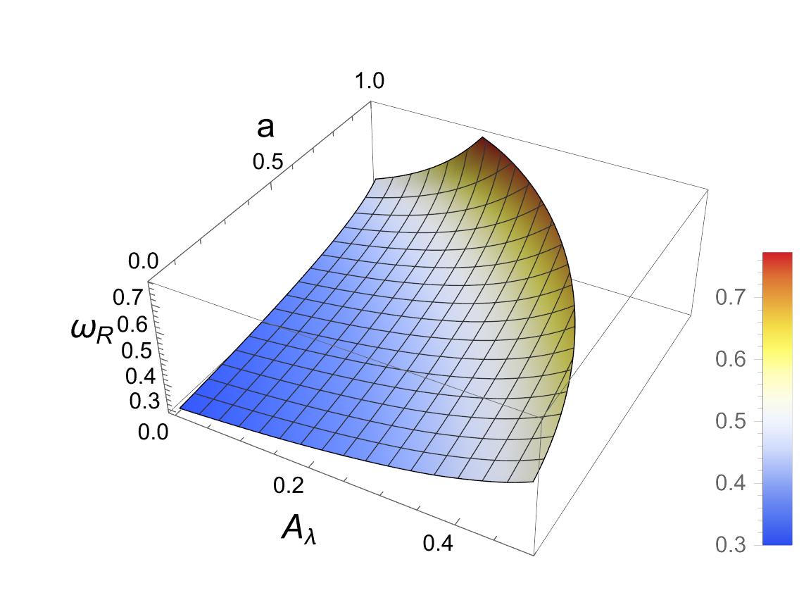
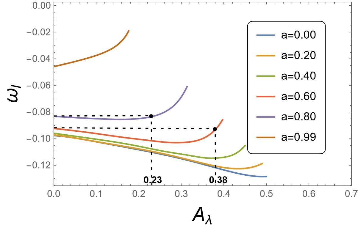
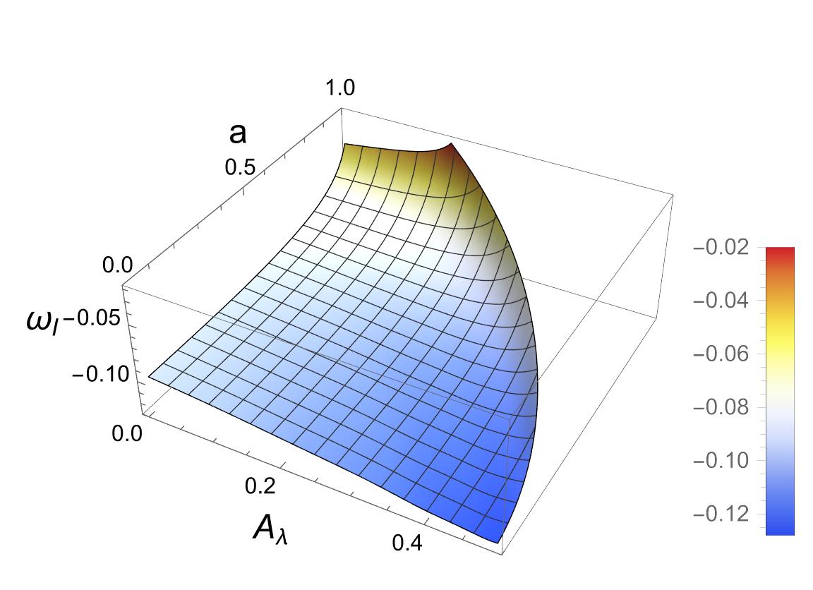
Figure 3: QNM frequencies $\omega$ as a function of regularization parameter $A_{\lambda}$ with a varying angular momentum, $a=0$, $0.3$, $0.6$, $0.9$, and $0.99$, where $M_{\rm B}=1$ and $\mu=0$ are set, and the mode of $l=1=m$ is chosen. In diagram (c), if we take $a=0.60$ as an example, we can see that $|\omega_{\rm I}|$ is smaller than that of the Kerr case ($A_{\lambda}=0$) when $A_{\lambda}>0.38$, and that it is larger than that of the Kerr case ($A_{\lambda}=0$) when $A_{\lambda}<0.38$.

Our analyses reveal that the quantum parameter $A_{\lambda}$ has a significant impact on the QNMs of massless scalar field perturbations in Tab. 1, where we present data on how the QNMs change with respect to the quantum parameter $A_{\lambda}$ for both $l=1=m$ and $l=2=m$ modes when $a=0.1$ and $M_{\rm B}=1$ are set. In the two modes, the real parts $\omega_{\rm R}$ grow with an increase of the quantum parameter $A_{\lambda}$. This indicates that an increase of $A_{\lambda}$ amplifies the oscillation frequencies of scalar fields. For example, in the mode of $l=1=m$, the real part corresponding to $A_{\lambda}=0.45$ is 1.69 times larger than that corresponding to $A_{\lambda}=0$. Furthermore, as $A_{\lambda}$ increases, the absolute value of imaginary parts $|\omega_{\rm I}|$ also increases, indicating a faster dissipation of waveforms. For instance, in the mode of $l=1=m$, $|\omega_{\rm I}|$ corresponding to $A_{\lambda}=0.45$ is 1.29 times larger than that corresponding to $A_{\lambda}=0$. These results highlight the significance of quantum parameter $A_{\lambda}$ in influencing the behaviors of QNMs of massless scalar field perturbations.

Now we present the influence of $A_{\lambda}$ on the QNMs of massless scalar field perturbations under different values of $a$ in Fig. 3, where the maximum value of $A_{\lambda}$ is determined by Eq. (15). Here we take the mode of $l=1=m$ as an example and set $M_{\rm B}=1$. As shown in Figs. 3 and 3, the real parts of QNMs always increase with an increase of $A_{\lambda}$ under a fixed $a$, where the largest real part is $\omega_{\rm R}=0.7828$, located at $a=1$ and $A_{\lambda}=0.125$, and it corresponds to the extreme configuration of rLQGBHs with the greatest angular momentum, $a_{\rm Max}=1$. Moreover, as shown in Figs. 3 and 3, $A_{\lambda}$ has diverse effects on $|\omega_{\rm I}|$ under different values of $a$, which can be divided into three categories:

• When $0<a\leq 0.48$, $|\omega_{\rm I}|$ increases at first and then decreases when $A_{\lambda}$ grows. Within the entire range of $A_{\lambda}$, $|\omega_{\rm I}|$ is always larger than that corresponding to $A_{\lambda}=0$. From a physical perspective, a non-vanishing $A_{\lambda}$ gives rise to a faster decay of massless scalar fields than the case of vanishing $A_{\lambda}$, thereby making the spacetime more unstable. Note that an rLQGBH reaches its extreme configuration when $A_{\lambda}$ takes its maximum value, see Eq. (15), and it reduces to a Kerr black hole when $A_{\lambda}$ equals zero. When $a$ increases, the gap between $|\omega_{\rm I}|$ of an extreme rLQGBH and that of a Kerr black hole is getting smaller and smaller, and finally it disappears when $a=0.48$.

• When $0.48<a\leq 0.82$, $|\omega_{\rm I}|$ also initially increases and then decreases when $A_{\lambda}$ grows. However, when $A_{\lambda}$ exceeds some specific value that depends on $a$, $|\omega_{\rm I}|$ is smaller than that of the Kerr case. For instance, we show that this specific value equals $0.38$ when $a=0.60$ or $0.23$ when $a=0.80$ in Fig. 3. Therefore, $A_{\lambda}$ plays the role in promoting the stability of spacetime when $A_{\lambda}$ is larger than this specific value, but it plays the role in diminishing the stability of spacetime when $A_{\lambda}$ is smaller than this specific value. Additionally, this specific value becomes small when $a$ increases, and it reaches zero when $a=0.82$.

• When $0.82<a\leq 1.00$, $|\omega_{\rm I}|$ decreases monotonically when $A_{\lambda}$ grows, implying that $A_{\lambda}$ plays the role in promoting the stability of spacetime. When $a=1$ and $A_{\lambda}=0.125$, $|\omega_{\rm I}|$ reaches the minimum value, $|\omega_{\rm I}|_{\rm Min}=0.0202$.

In addition, we present the influence of $A_{\lambda}$ on the QNMs of massless scalar field perturbations under different values of $a$ for the mode of $l=2=m$ in Fig. 4, where the maximum value of $A_{\lambda}$ is also determined by Eq. (15). In general, the influence of $A_{\lambda}$ on QNMs in the mode of $l=2=m$ is similar to that in the mode of $l=1=m$, i.e., the former differs from the latter just in numerical differences. For the real parts of QNMs, the former is significantly larger than the latter. But for the absolute value of imaginary parts, the difference between the two modes is very small. Similarly, for the mode of $l=2=m$, the influence of $A_{\lambda}$ on $|\omega_{\rm I}|$ can also be divided into three categories for a varying $a$: $0<a\leq 0.49$, $0.49<a\leq 0.84$, and $0.84<a\leq 1.00$. From Fig. 4 it is clear that the relations between $\omega_{\rm R}$ ($|\omega_{\rm I}|$) and $A_{\lambda}$ are quite similar in the two modes.

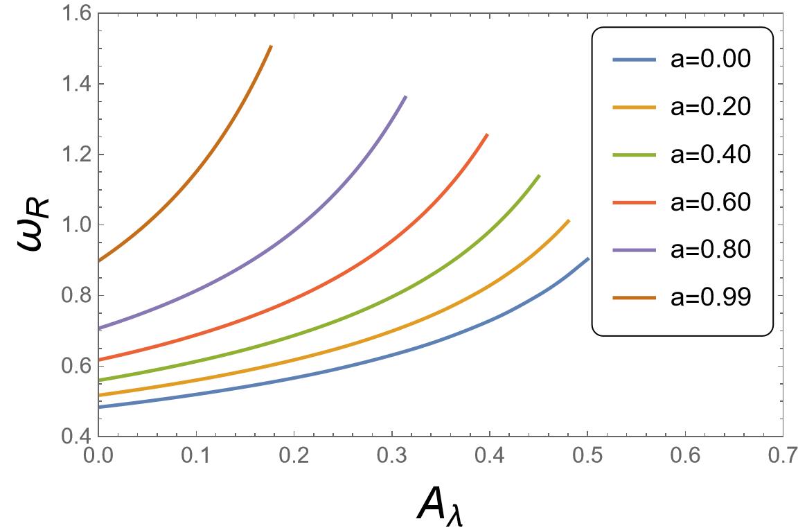
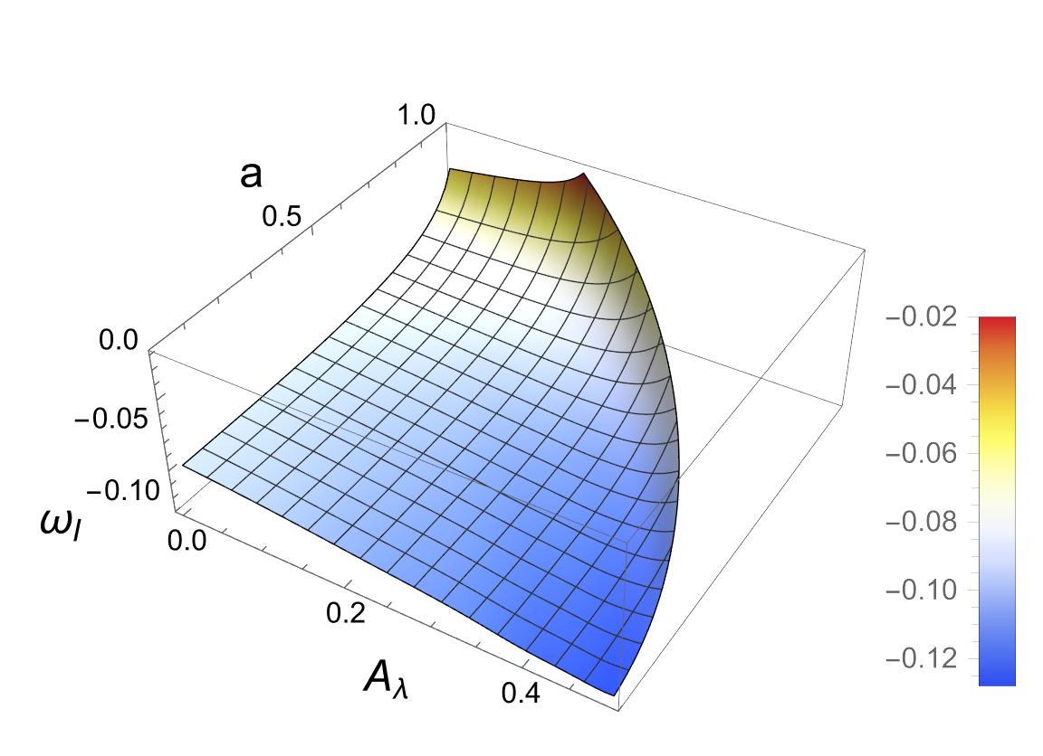
Figure 4: QNM frequencies $\omega$ as a function of quantum parameter $A_{\lambda}$ with a varying angular momentum, $a=0$, $0.3$, $0.6$, $0.9$, and $0.99$, where $M_{\rm B}=1$ and $\mu=0$ are set, and the mode of $l=2=m$ is chosen. In diagram (c), if we take $a=0.60$ as an example, we can see that $|\omega_{\rm I}|$ is smaller than that of the Kerr case ($A_{\lambda}=0$) when $A_{\lambda}>0.37$, and that it is larger than that of the Kerr case ($A_{\lambda}=0$) when $A_{\lambda}<0.37$.

In Fig.5, we demonstrate the relationship between the QNMs and the quantum parameter $A_{\lambda}$ under a varying scalar field mass $\mu$. It can be observed for a fixed $A_{\lambda}$ that the presence of $\mu$ leads to an increase of the real parts of $\omega$ but a decrease of the absolute value of imaginary parts. This implies that the massive scalar field perturbations around rLQGBHs oscillate faster but decay more slowly compared to the massless case, and that the mass $\mu$ plays the role in promoting the stability of spacetime. When $A_{\lambda}=0$, i.e., in Kerr black holes $\mu$ has the greatest influence on the QNMs. When $A_{\lambda}$ gradually increases, the influence of $\mu$ gradually decreases. Therefore, a non-vanishing $A_{\lambda}$ makes $\mu$ have a weaker effect on promoting the spacetime stability than a vanishing $A_{\lambda}$ does.

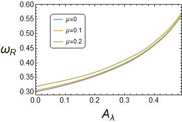
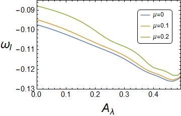
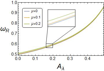
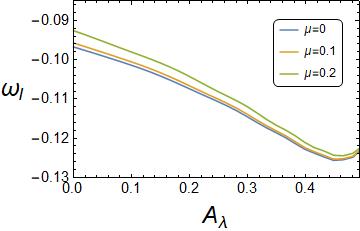
Figure 5: QNM frequencies $\omega$ as a function of quantum parameter $A_{\lambda}$ with different masses of scalar fields, $\mu=0$, $0.1$, and $0.2$, where $a=0.1$, $M_{\rm B}=1$, and $n=0$ are set, the upper two diagrams correspond to the mode of $l=1=m$, and the lower two diagrams the mode of $l=2=m$.

5 Superradiance

When a free scalar field is incident on a black hole, the incident wave will be decomposed into two parts, a reflected wave and a transmitted wave, due to the scattering effect of potential barriers near the black hole. The boundary conditions of this process include pure ingoing wave at the event horizon and both ingoing wave and outgoing wave at the spatial infinity, where the ingoing wave at the event horizon corresponds to the transmitted wave, while the ingoing wave and outgoing wave at the spatial infinity correspond to the incident wave and reflected wave, respectively. The energy of reflected waves is greater than the energy of incident waves when the frequency $\omega$ of incident scalar fields satisfies [49] the following conditions:

$$m\Omega_{\rm H}>\omega>\mu,$$ (51)

where

$$\Omega_{\rm H}=\frac{a}{h_{+}^{2}-6A_{\lambda}M_{\rm B}^{2}+a^{2}}$$ (52)

is the angular velocity of scalar particles at the outer event horizon $h_{+}$ determined by Eq. (14) for rLQGBHs. It is worth noting that the frequency $\omega$ of scalar fields is always real owing to the special boundary conditions of scattering processes. This phenomenon of energy amplification is called [18] superradiance. Next we study how the energy amplification factor is affected by the quantum parameter $A_{\lambda}$.

5.1 Numerical method

In terms of the boundary conditions mentioned above, the radial equation of motion Eq. (36) takes the asymptotic solution at the spatial infinity as follows:

$$R(h)\sim\mathscr{I}\frac{1}{h}\mathrm{e}^{-qh}h^{-M_{\rm B}(\mu^{2}-2\omega^{2})/q}+\mathscr{R}\frac{1}{h}\mathrm{e}^{qh}h^{M_{\rm B}(\mu^{2}-2\omega^{2})/q},$$ (53)

where $\mathscr{I}$ and $\mathscr{R}$ stand for the incident and reflection amplitudes, respectively. Moreover, the asymptotic wave function near the outer horizon $h_{+}$ reads

$$R(h)\sim\mathscr{T}(h-h_{+})^{i\alpha},$$ (54)

where $\mathscr{T}$ is the transmission amplitude. Then the amplification factor is given [18] by

$$Z_{lm}=\frac{\mathrm{d}E_{\rm out}}{\mathrm{d}E_{\rm in}}=\left|\frac{\mathscr{R}}{\mathscr{I}}\right|^{2}-1.$$ (55)

Following the shooting method outlined in Sec. 4.3, we establish the relationship among $\mathscr{I}$, $\mathscr{R}$, and $\mathscr{T}$, and thus give the amplification factor of superradiance.

5.2 Results

In Fig. 6 we present the relations between the amplification factor and $\omega$ under a varying $A_{\lambda}$ for a massless incident particle and a massive one with mass $\mu=0.2$, respectively. In the region where the superradiance effect appears, the energy amplification factor always increases at first and then decreases as the particle frequency $\omega$ grows. On the boundaries of the region, $\omega=\mu$ and $\omega=m\Omega_{\mathrm{H}}$, see Eq. (51) with $M_{\rm B}=1$, the amplification factor is always zero. Moreover, the amplification factor decreases as the particle mass $\mu$ increases, indicating that the superradiance effect is inhibited by particle mass.

The influence of quantum parameter $A_{\lambda}$ on the amplification factor varies with the particle frequency $\omega$. When the particle frequency $\omega$ is low, a small $A_{\lambda}$ leads to an amplification factor that is larger than that led by a big $A_{\lambda}$. The specific situation can be observed in the small picture of Fig. 6, where an increase of $A_{\lambda}$ restrains the superradiance effect in the region of small $\omega$. However, as $\omega$ gradually increases, the amplification factor associated with a small $A_{\lambda}$ is gradually surpassed by the amplification factor associated with a big $A_{\lambda}$. Ultimately, a larger $A_{\lambda}$ results in a greater peak of amplification factors. On the whole, an increase of $A_{\lambda}$ plays the role in promoting the superradiance effect.

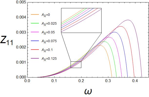
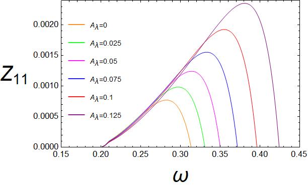
Figure 6: Amplification factor with respect to the frequency of scalar fields for the mode of $l=1=m$ in rLQGBHs, where $n=0$, $M_{\rm B}=1$, and $a=0.9$ are set, and the left diagram corresponds to the case of massless scalar fields, $\mu=0$, and the right one to the case of massive scalar fields with mass $\mu=0.2$.

6 Conclusion

In the present work, we investigate the scalar field perturbations in the background of rLQGBHs. In order to analyze the time domain evolution of scalar fields around rLQGBHs, we employ the hyperbolic foliation Eq. (23) to overcome numerical issues at the boundaries and obtain the time domain evolution profiles. By comparing the evolution profiles of scalar fields under different quantum parameter $A_{\lambda}$, we observe that the introduction of $A_{\lambda}$ has no impact on the outburst and late-time tail stages, but affects the damping oscillation stage significantly.

In order to gain a deeper understanding of the influence of $A_{\lambda}$ on scalar field evolution, we extract the QNMs of scalar field perturbations from damping oscillations by the Prony method, the 4th-order WKB method and the shooting method. We point out that the Prony method has the highest precision among the three methods, but the shooting method is the most efficient in numerical simulations. Moreover, we find that the influence of scalar field mass $\mu$ on the QNMs becomes more pronounced for a larger $A_{\lambda}$. Further, we investigate the impact of $A_{\lambda}$ on the QNMs for different angular momentum $a$. Interestingly, we observe that the effect of $A_{\lambda}$ on the QNMs varies with different values of angular momenta.

We also analyze the impact of $A_{\lambda}$ on the superradiance effect in rLQGBHs. We find that $A_{\lambda}$ expands the frequency range of superradiance effects and enhances the efficiency of superradiant amplification significantly when $\omega\sim m\Omega_{\rm H}$.

Based on our investigations on QNMs and superradiance, we conclude that the quantum parameter plays an important role in determining the dynamics of ultralight massive scalar fields. Our results provide some new understanding of rLQGBHs. Considering that the metric of rLQGBHs can also describe rotating LQG wormholes, we plan to analyze the dynamical behaviors of rotating LQG wormholes. The issue probably lies in solving the radial equation of motion under the special boundary conditions of rotating LQG wormholes. We leave it in our future research.

References

- [1] S. W. Hawking. Black hole explosions. Nature, 248:30–31, 1974. doi:10.1038/248030a0.
- [2] Roger Penrose. Gravitational collapse: The role of general relativity. Nuovo Cimento Rivista Serie, 1:252, 1969. doi:10.1103/PhysRevLett.14.57.
- [3] Chen Lan, Hao Yang, Yang Guo, and Yan-Gang Miao. Regular Black Holes: A Short Topic Review. Int. J. Theor. Phys., 62(9):202, 2023. arXiv:2303.11696, doi:10.1007/s10773-023-05454-1.
- [4] James Bardeen. Non-singular general relativistic gravitational collapse. In Proceedings of the 5th International Conference on Gravitation and the Theory of Relativity, page 87, 1968.
- [5] Alfio Bonanno and Martin Reuter. Renormalization group improved black hole space-times. Phys. Rev. D, 62:043008, 2000. arXiv:hep-th/0002196, doi:10.1103/PhysRevD.62.043008.
- [6] Benjamin Koch and Frank Saueressig. Black holes within Asymptotic Safety. Int. J. Mod. Phys. A, 29(8):1430011, 2014. arXiv:1401.4452, doi:10.1142/S0217751X14300117.
- [7] Mariam Bouhmadi-López, Che-Yu Chen, Xiao Yan Chew, Yen Chin Ong, and Dong-Han Yeom. Regular Black Hole Interior Spacetime Supported by Three-Form Field. Eur. Phys. J. C, 81(4):278, 2021. arXiv:2005.13260, doi:10.1140/epjc/s10052-021-09080-1.
- [8] Leonardo Modesto. Loop quantum black hole. Class. Quant. Grav., 23:5587–5602, 2006. arXiv:gr-qc/0509078, doi:10.1088/0264-9381/23/18/006.
- [9] Rodolfo Gambini and Jorge Pullin. Loop quantization of the Schwarzschild black hole. Phys. Rev. Lett., 110(21):211301, 2013. arXiv:1302.5265, doi:10.1103/PhysRevLett.110.211301.
- [10] Norbert Bodendorfer, Fabio M. Mele, and Johannes Münch. (b,v)-type variables for black to white hole transitions in effective loop quantum gravity. Phys. Lett. B, 819:136390, 2021. arXiv:1911.12646, doi:10.1016/j.physletb.2021.136390.
- [11] Norbert Bodendorfer, Fabio M. Mele, and Johannes Münch. Mass and Horizon Dirac Observables in Effective Models of Quantum Black-to-White Hole Transition. Class. Quant. Grav., 38(9):095002, 2021. arXiv:1912.00774, doi:10.1088/1361-6382/abe05d.
- [12] Suddhasattwa Brahma, Che-Yu Chen, and Dong-han Yeom. Testing Loop Quantum Gravity from Observational Consequences of Nonsingular Rotating Black Holes. Phys. Rev. Lett., 126(18):181301, 2021. arXiv:2012.08785, doi:10.1103/PhysRevLett.126.181301.
- [13] Misba Afrin, Sunny Vagnozzi, and Sushant G. Ghosh. Tests of Loop Quantum Gravity from the Event Horizon Telescope Results of Sgr A*. Astrophys. J., 944(2):149, 2023. arXiv:2209.12584, doi:10.3847/1538-4357/acb334.
- [14] R. A. Konoplya and A. Zhidenko. Quasinormal modes of black holes: From astrophysics to string theory. Rev. Mod. Phys., 83:793–836, 2011. arXiv:1102.4014, doi:10.1103/RevModPhys.83.793.
- [15] K. D. Kokkotas and B. G. Schmidt. Quasi-normal modes of stars and black holes. Living Reviews in Relativity, 2(1):2, 1999. arXiv:gr-qc/9909058, doi:10.12942/lrr-1999-2.
- [16] Zhen Li. Scalar perturbation around rotating regular black hole: Superradiance instability and quasinormal modes. Phys. Rev. D, 107(4):044013, 2023. arXiv:2210.14062, doi:10.1103/PhysRevD.107.044013.
- [17] Edgardo Franzin, Stefano Liberati, Jacopo Mazza, Ramit Dey, and Sumanta Chakraborty. Scalar perturbations around rotating regular black holes and wormholes: Quasinormal modes, ergoregion instability, and superradiance. Phys. Rev. D, 105(12):124051, 2022. arXiv:2201.01650, doi:10.1103/PhysRevD.105.124051.
- [18] Richard Brito, Vitor Cardoso, and Paolo Pani. Superradiance: New Frontiers in Black Hole Physics. Lect. Notes Phys., 906:pp.1–237, 2015. arXiv:1501.06570, doi:10.1007/978-3-319-19000-6.
- [19] Vitor Cardoso, Seth Hopper, Caio FB Macedo, Carlos Palenzuela, and Paolo Pani. Gravitational-wave signatures of exotic compact objects and of quantum corrections at the horizon scale. Physical Review D, 94(8):084031, 2016. URL: https://doi.org/10.1103/PhysRevD.94.084031, arXiv:1608.08637, doi:10.1103/PhysRevD.94.084031.
- [20] Davide Gerosa and Maya Fishbach. Hierarchical mergers of stellar-mass black holes and their gravitational-wave signatures. Nature Astronomy, 5(8):749–760, 2021. doi:10.1038/s41550-021-01398-w.
- [21] Lukas R. Weih, Matthias Hanauske, and Luciano Rezzolla. Postmerger Gravitational-Wave Signatures of Phase Transitions in Binary Mergers. Phys. Rev. Lett., 124(17):171103, 2020. arXiv:1912.09340, doi:10.1103/PhysRevLett.124.171103.
- [22] W. H. Press and S. A. Teukolsky. Floating orbits, superradiant scattering and the black-hole bomb. Nature, 238(5362):211–212, 1972. doi:10.1038/238211a0.
- [23] J. D. Bekenstein. Extraction of energy and charge from a black hole. Physical Review D, 7(8):949–953, 1973. doi:10.1103/PhysRevD.7.949.
- [24] Y. B. Zeldovich. Amplification of cylindrical electromagnetic waves reflected from a rotating body. Soviet Journal of Experimental and Theoretical Physics Letters, 14(3):180–181, 1971.
- [25] A. A. Starobinsky and S. M. Churilov. Amplification of electromagnetic and gravitational waves scattered by a rotating ”black hole”. Soviet Physics JETP, 38(1):1–5, 1973.
- [26] William E. East. Massive Boson Superradiant Instability of Black Holes: Nonlinear Growth, Saturation, and Gravitational Radiation. Phys. Rev. Lett., 121(13):131104, 2018. arXiv:1807.00043, doi:10.1103/PhysRevLett.121.131104.
- [27] Edward W Leaver. An analytic representation for the quasi-normal modes of kerr black holes. Proceedings of the Royal Society of London. A. Mathematical and Physical Sciences, 402(1823):285–298, 1985. doi:10.1098/rspa.1985.0119.
- [28] Mustapha Azreg-Aïnou. Generating rotating regular black hole solutions without complexification. Phys. Rev. D, 90(6):064041, 2014. arXiv:1405.2569, doi:10.1103/PhysRevD.90.064041.
- [29] Ingrid Thuestad, Gaurav Khanna, and Richard H. Price. Scalar fields in black hole spacetimes. Physical Review D, 96(2):024020, 2017. arXiv:arXiv:1704.05096, doi:10.1103/PhysRevD.96.024020.
- [30] Shao-Jun Zhang, Bin Wang, Anzhong Wang, and Joel F Saavedra. Object picture of scalar field perturbation on kerr black hole in scalar-einstein-gauss-bonnet theory. Physical Review D, 102(12):124056, 2020. arXiv:2007.10348, doi:10.1103/PhysRevD.102.124056.
- [31] Anıl Zenginoglu. Hyperboloidal foliations and scri-fixing. Classical Quantum Gravity, 25(14):145002, 2008. arXiv:0805.4895, doi:10.1088/0264-9381/25/14/145002.
- [32] Anıl Zenginoglu. A hyperboloidal study of tail decay rates for scalar and yang-mills fields. Classical Quantum Gravity, 25(17):175013, 2008. arXiv:0806.1642, doi:10.1088/0264-9381/25/17/175013.
- [33] Anıl Zenginoglu. Hyperboloidal evolution with the einstein equations. Classical Quantum Gravity, 25(19):195025, 2008. arXiv:0807.4170, doi:10.1088/0264-9381/25/19/195025.
- [34] Anıl Zenginoglu, Dario Nunez, and Sascha Husa. Gravitational perturbations of schwarzschild spacetime at null infinity and the hyperboloidal initial value problem. Classical Quantum Gravity, 26(3):035009, 2009. arXiv:0809.4726, doi:10.1088/0264-9381/26/3/035009.
- [35] Anıl Zenginoglu and Manuel Tiglio. Spacelike matching to null infinity. Physical Review D, 80(2):024044, 2009. doi:10.1103/PhysRevD.80.024044.
- [36] Anıl Zenginoglu. Asymptotics of black hole perturbations. Classical Quantum Gravity, 27(4):045015, 2010. doi:10.1088/0264-9381/27/4/045015.
- [37] Anıl Zenginoglu. Hyperboloidal layers for hyperbolic equations on unbounded domains. Journal of Computational Physics, 230(6):2286, 2011. doi:10.1016/j.jcp.2010.12.007.
- [38] Anıl Zenginoglu. A geometric framework for black hole perturbations. Physical Review D, 83(12):127502, 2011. doi:10.1103/PhysRevD.83.127502.
- [39] Enno Harms, Sebastiano Bernuzzi, Alessandro Nagar, and An Zenginoglu. A new gravitational wave generation algorithm for particle perturbations of the Kerr spacetime. Class. Quant. Grav., 31(24):245004, 2014. arXiv:1406.5983, doi:10.1088/0264-9381/31/24/245004.
- [40] Emanuele Berti, Vitor Cardoso, Jose A. Gonzalez, and Ulrich Sperhake. Mining information from binary black hole mergers: A Comparison of estimation methods for complex exponentials in noise. Phys. Rev. D, 75:124017, 2007. arXiv:gr-qc/0701086, doi:10.1103/PhysRevD.75.124017.
- [41] S. Chandrasekhar and Steven L. Detweiler. The quasi-normal modes of the Schwarzschild black hole. Proc. Roy. Soc. Lond. A, 344:441–452, 1975. doi:10.1098/rspa.1975.0112.
- [42] C. Molina, Paolo Pani, Vitor Cardoso, and Leonardo Gualtieri. Gravitational signature of Schwarzschild black holes in dynamical Chern-Simons gravity. Phys. Rev. D, 81:124021, 2010. arXiv:1004.4007, doi:10.1103/PhysRevD.81.124021.
- [43] Sai Iyer. BLACK HOLE NORMAL MODES: A WKB APPROACH. 2. SCHWARZSCHILD BLACK HOLES. Phys. Rev. D, 35:3632, 1987. doi:10.1103/PhysRevD.35.3632.
- [44] Edward Seidel and Sai Iyer. BLACK HOLE NORMAL MODES: A WKB APPROACH. 4. KERR BLACK HOLES. Phys. Rev. D, 41:374–382, 1990. doi:10.1103/PhysRevD.41.374.
- [45] R. A. Konoplya, A. Zhidenko, and A. F. Zinhailo. Higher order WKB formula for quasinormal modes and grey-body factors: recipes for quick and accurate calculations. Class. Quant. Grav., 36:155002, 2019. arXiv:1904.10333, doi:10.1088/1361-6382/ab2e25.
- [46] R. A. Konoplya. Quasinormal behavior of the d-dimensional Schwarzschild black hole and higher order WKB approach. Phys. Rev. D, 68:024018, 2003. arXiv:gr-qc/0303052, doi:10.1103/PhysRevD.68.024018.
- [47] Edward Seidel. A comment on the eigenvalues of spin-weighted spheroidal functions. Classical and Quantum Gravity, 6(7):1057, 1989. doi:10.1088/0264-9381/6/7/012.
- [48] RA Konoplya and AV Zhidenko. Stability and quasinormal modes of the massive scalar field around kerr black holes. Physical Review D, 73(12):124040, 2006. arXiv:gr-qc/0605013, doi:10.1103/PhysRevD.73.124040.
- [49] Si-Jiang Yang, Yu-Peng Zhang, Shao-Wen Wei, and Yu-Xiao Liu. Destroying the event horizon of a nonsingular rotating quantum-corrected black hole. JHEP, 04:066, 2022. arXiv:2201.03381, doi:10.1007/JHEP04(2022)066.