Feasibility-Guaranteed Safety Critical Control with Applications to
Heterogeneous Platoons

Abstract

This paper studies safety and feasibility guarantees for systems with tight control bounds. It has been shown that stabilizing an affine control system while optimizing a quadratic cost and satisfying state and control constraints can be mapped to a sequence of Quadratic Programs (QPs) using Control Barrier Functions (CBF) and Control Lyapunov Functions (CLF). One of the main challenges in this method is that the QP could easily become infeasible under safety constraints of high relative degree, especially under tight control bounds. Recent work focused on deriving sufficient conditions for guaranteeing feasibility. The existing results are case-dependent. In this paper, we consider the general case and define a feasibility constraint, and propose a new type of CBF to enforce the feasibility constraint. Our method guarantees the feasibility of the above mentioned QPs, while satisfying safety requirements. We demonstrate the advantages of using the proposed method on a heterogeneous Adaptive Cruise Control (ACC) platoon with tight control bounds, and compare our method to existing CBF-CLF approaches. The results show that our proposed approach can generate gradually transitioned control with guaranteed feasibility and safety.

I Introduction

Safety is one of the primary concerns in the design and operation of autonomous systems. Many existing works enforce safety as constraints in optimal control problems using barrier and control barrier functions. Barrier functions (BFs) are Lyapunov-like functions [1] whose use can be traced back to optimization problems [2]. They have been utilized to prove set invariance [3], [4] to derive multi-objective control [5], [6], and to control multi-robot systems [7].

Control Barrier Functions (CBFs) are extensions of BFs used to enforce safety, i.e., rendering a set forward invariant, for an affine control system. It was proved in [8] that if a CBF for a safe set satisfies Lyapunov-like conditions, then this set is forward invariant and safety is guaranteed. It has also been shown that stabilizing an affine control system to admissible states, while minimizing a quadratic cost subject to state and control constraints, can be mapped to a sequence of Quadratic Programs (QPs) [8] by unifying CBFs and Control Lyapunov Functions (CLFs) [9]. In its original form, this approach, which in this paper we will refer to as CBF-CLF, works only for safety constraints with relative degree one. Exponential CBFs [10] were introduced to accommodate higher relative degrees. A more general form of exponential CBFs, called High Order CBFs (HOCBFs), has been proposed in [11]. The CBF-CLF method has been widely used to enforce safety in many applications, including rehabilitative system control [12], adaptive cruise control [8], humanoid robot walking [13] and robot swarming [14]. However, the aforementioned CBF-CLF QP might be infeasible in the presence of tight or time-varying control bounds due to the conflicts between CBF constraints and control bounds.

There are several approaches that aim to enhance the feasibility of the CBF-CLF method, while guaranteeing safety and satisfy the control bounds. The authors of [15] formulate CBFs as constraints in Nonlinear Model Predictive Control (NMPC) framework, which allows the controller to predict future state information up to a horizon larger than one. This leads to a less aggressive control strategy than the original one-step ahead approach. However, the corresponding optimization is overall nonlinear and non-convex, and the computation is expensive. An iterative approach based on a convex MPC with linearized, discrete-time CBFs was proposed in [16]. However, the linearization affects the safety guarantee and global optimality. The works in [17, 18, 19, 20] are based on a set of backup policies that are used to extend the safe set to a larger viable set to enhance the feasible space of the system in a finite time horizon under input constraints. This backup approach has further been generalized to infinite time horizons [21], [22]. One limitation of these approaches is that they require prior knowledge on backup sets, policies, or nominal control laws. Another limitation is that these approaches may introduce overly aggressive or conservative control strategies.

Adaptive CBFs (aCBFs) [23] have been proposed for time-varying control bounds by introducing penalty functions in the HOCBFs constraints. These provide flexible and adaptive control strategies over time. An Auxiliary-Variable Adaptive CBF (AVCBF) method was proposed in [24], which preserves the adaptive property of aCBFs [23] while generating smooth control policies near the boundaries of safe sets. The smooth control policies help to regulate a system’s behavior with gradually transitioned control and output. AVCBFs also require less additional constraints and simpler parameter tuning compared to aCBFs [23]. These approaches, however, cannot guarantee the feasibility of the optimization by only making some hard constraints soft or by extending the feasible spaces of the safe sets. The work in [25] provided sufficient conditions to guarantee the feasibility of the CBF-CLF QPs without softening hard constraints. However, the method was developed for a particular case, and it is not clear how it can be generalized.

In this paper, we generalize the method from [25] by proposing a new type of CBF for safety-critical control problems. Specifically, we define a feasibility constraint, an auxiliary variable, and a CBF-based equation for the auxiliary variable that works for general affine control systems. We guarantee feasibility and safety under tight control bounds. Moreover, the generated control policy is smooth without sharp transition. We demonstrate the effectiveness of the proposed method on an adaptive cruise control problem with tight control bounds, and compare it to the existing CBF-CLF approaches. The results show that our proposed approach can generate smoother control with guaranteed feasibility and safety.

II Preliminaries

Consider an affine control system of the form

$$\dot{\bm{x}}=f(\bm{x})+g(\bm{x})\bm{u},$$ (1)

where $\bm{x}\in\mathbb{R}^{n},f:\mathbb{R}^{n}\to\mathbb{R}^{n}$ and $g:\mathbb{R}^{n}\to\mathbb{R}^{n\times q}$ are locally Lipschitz, and $\bm{u}\in\mathcal{U}\subset\mathbb{R}^{q}$, where $\mathcal{U}$ denotes the control limitation set, which is assumed to be in the form:

$$\mathcal{U}\coloneqq\{\bm{u}\in\mathbb{R}^{q}:\bm{u}_{min}\leq\bm{u}\leq\bm{u}_{max}\},$$ (2)

with $\bm{u}_{min},\bm{u}_{max}\in\mathbb{R}^{q}$ (vector inequalities are interpreted componentwise).

Definition 1 (Class $\kappa$ function [26]).

A continuous function $\alpha:[0,a)\to[0,+\infty],a>0$ is called a class $\kappa$ function if it is strictly increasing and $\alpha(0)=0.$

Definition 2.

A set $\mathcal{C}\subset\mathbb{R}^{n}$ is forward invariant for system (1) if its solutions for some $\bm{u}\in\mathcal{U}$ starting from any $\bm{x}(0)\in\mathcal{C}$ satisfy $\bm{x}(t)\in\mathcal{C},\forall t\geq 0.$

Definition 3.

The relative degree of a differentiable function $b:\mathbb{R}^{n}\to\mathbb{R}$ is the minimum number of times we need to differentiate it along dynamics (1) until any component of $\bm{u}$ explicitly shows in the corresponding derivative.

In this paper, a safety requirement is defined as $b(\bm{x})\geq 0$, and safety is the forward invariance of the set $\mathcal{C}\coloneqq\{\bm{x}\in\mathbb{R}^{n}:b(\bm{x})\geq 0\}$. The relative degree of function $b$ is also referred to as the relative degree of safety requirement $b(\bm{x})\geq 0$. For a requirement $b(\bm{x})\geq 0$ with relative degree $m$ and $\psi_{0}(\bm{x})\coloneqq b(\bm{x}),$ we define a sequence of functions $\psi_{i}:\mathbb{R}^{n}\to\mathbb{R},\ i\in\{1,...,m\}$ as

$$\psi_{i}(\bm{x})\coloneqq\dot{\psi}_{i-1}(\bm{x})+\alpha_{i}(\psi_{i-1}(\bm{x})),\ i\in\{1,...,m\},$$ (3)

where $\alpha_{i}(\cdot),\ i\in\{1,...,m\}$ denotes a $(m-i)^{th}$ order differentiable class $\kappa$ function. We further define a sequence of sets $\mathcal{C}_{i}$ based on (3) as

$$\mathcal{C}_{i}\coloneqq\{\bm{x}\in\mathbb{R}^{n}:\psi_{i}(\bm{x})\geq 0\},\ i\in\{0,...,m-1\}.$$ (4)

Definition 4 (HOCBF [11]).

Let $\psi_{i}(\bm{x}),\ i\in\{1,...,m\}$ be defined by (3) and $\mathcal{C}_{i},\ i\in\{0,...,m-1\}$ be defined by (4). A function $b:\mathbb{R}^{n}\to\mathbb{R}$ is a High Order Control Barrier Function (HOCBF) with relative degree $m$ for system (1) if there exist $(m-i)^{th}$ order differentiable class $\kappa$ functions $\alpha_{i},\ i\in\{1,...,m\}$ such that

$$\begin{split}\sup_{\bm{u}\in\mathcal{U}}[L_{f}^{m}b(\bm{x})+L_{g}L_{f}^{m-1}b(\bm{x})\bm{u}+O(b(\bm{x}))+\\ \alpha_{m}(\psi_{m-1}(\bm{x}))]\geq 0,\end{split}$$ (5)

$\forall\bm{x}\in\mathcal{C}_{0}\cap,...,\cap\mathcal{C}_{m-1},$ where $L_{f}^{m}$ denotes the $m^{th}$ Lie derivative along $f$ and $L_{g}$ denotes the matrix of Lie derivatives along the columns of $g$; $O(\cdot)=\sum_{i=1}^{m-1}L_{f}^{i}(\alpha_{m-1}\circ\psi_{m-i-1})(\bm{x})$ contains the remaining Lie derivatives along $f$ with degree less than or equal to $m-1$. $\psi_{i}(\bm{x})\geq 0$ is referred to as the $i^{th}$ order HOCBF inequality (constraint in optimization). We assume that $L_{g}L_{f}^{m-1}b(\bm{x})\bm{u}\neq 0$ on the boundary of set $\mathcal{C}_{0}\cap,...,\cap\mathcal{C}_{m-1}.$

Theorem 1 (Safety Guarantee [11]).

Given a HOCBF $b(\bm{x})$ from Def. 4 with corresponding sets $\mathcal{C}_{0},\dots,\mathcal{C}_{m-1}$ defined by (4), if $\bm{x}(0)\in\mathcal{C}_{0}\cap\dots\cap\mathcal{C}_{m-1},$ then any Lipschitz controller $\bm{u}$ that satisfies the inequality in (5), $\forall t\geq 0$ renders $\mathcal{C}_{0}\cap\dots\cap\mathcal{C}_{m-1}$ forward invariant for system (1), $i.e.,\bm{x}\in\mathcal{C}_{0}\cap\dots\cap\mathcal{C}_{m-1},\forall t\geq 0.$

Definition 5 (CLF [9]).

A continuously differentiable function $V:\mathbb{R}^{n}\to\mathbb{R}$ is an exponentially stabilizing Control Lyapunov Function (CLF) for system (1) if there exist constants $c_{1}>0,c_{2}>0,c_{3}>0$ such that for $\forall\bm{x}\in\mathbb{R}^{n},c_{1}\left\|\bm{x}\right\|^{2}\leq V(\bm{x})\leq c_{2}\left\|\bm{x}\right\|^{2},$

$$\inf_{\bm{u}\in\mathcal{U}}[L_{f}V(\bm{x})+L_{g}V(\bm{x})\bm{u}+c_{3}V(\bm{x})]\leq 0.$$ (6)

Some existing works [10],[11] combine HOCBFs (5) for systems with high relative degree with quadratic costs to form safety-critical optimization problems. The HOCBFs are used to ensure the forward invariance of sets related to safety requirement, therefore guaranteeing safety. CLFs (6) can also be incorporated (see [11],[23]) if exponential convergence of some states is desired. In these works, the control inputs are the decision (optimization) variables. Time is discretized into intervals, and an optimization problem with constraints given by HOCBFs (hard constraints) and CLFs (soft constraints) is solved in each time interval. The state value is fixed at the beginning of each interval, which results in linear constraints for the control - the resulting optimization problem is a QP. The optimal control obtained by solving each QP is applied at the beginning of the interval and held constant for the whole interval. During each interval, the state is updated using dynamics (1).

This method, which throughout this paper we will referred to as the CBF-CLF-QP method, works conditioned on the fact that solving the QP at every time interval is feasible. However, this is not guaranteed, and, in fact, unlikely to happen, if the control bounds in Eqn. (2) are tight. The authors of [25] proposed sufficient conditions to address the feasibility issue. In short, they created a feasibility constraint enforced by a first order CBF constraint (hard constraint) to avoid conflict between the $m^{th}$ order HOCBF constraint (hard constraint for safety) and control constraints (2) (hard constraint for control bounds). They made sure this first order CBF constraint was also compatible with the hard constraints for safety and control bounds. This method increases the overall feasibility of solving QPs since all hard constraints are compatible with each other. The method was successfully applied to a traffic merging control problem for Connected and Automated Vehicles (CAVs) [27]. However, these sufficient conditions are heavily dependent on the considered dynamics and constraints. In this paper, we show how we can find and satisfy sufficient conditions for the feasibility of the QPs given general dynamics and constraints.

III Problem Formulation and Approach

Our goal is to generate a control strategy for system (1) such that it converges to a desired state, some measure of spent energy is minimized, safety is satisfied, and control limitations are observed.

Objective: We consider the cost

$$\begin{split}J(\bm{u}(t))=\int_{0}^{T}D(\left\|\bm{u}(t)\right\|)dt+p\left\|\bm{x}(T)-\bm{x}_{e}\right\|^{2},\end{split}$$ (7)

where $\left\|\cdot\right\|$ denotes the 2-norm of a vector, $D(\cdot)$ is a strictly increasing function of its argument, and $T>0$ denotes the ending time; $p>0$ denotes a weight factor and $\bm{x}_{e}\in\mathbb{R}^{n}$ is a desired state, which is assumed to be an equilibrium for system (1).

Safety Requirement: System (1) should always satisfy one or more safety requirements of the form:

$$b(\bm{x})\geq 0,\bm{x}\in\mathbb{R}^{n},\forall t\in[0,T],$$ (8)

where $b:\mathbb{R}^{n}\to\mathbb{R}$ is assumed to be a continuously differentiable equation.

Control Limitations: The controller $\bm{u}$ should always satisfy (2) for all $t\in[0,T].$

A control policy is feasible if (8) and (2) are strictly satisfied $\forall t\in[0,T].$ In this paper, we consider the following problem:

Problem 1.

Find a feasible control policy for system (1) such that cost (7) is minimized.

Approach: We define a HOCBF to enforce (8). We also use a relaxed CLF to realize the state convergence in (7). Since the cost is quadratic in $\bm{u}$, we can formulate Prob. 1 using CBF-CLF-QPs:

$$\begin{split}\min_{u(t),\delta(t)}\int_{0}^{T}(\left\|\bm{u}(t)\right\|^{2}+p\delta^{2}(t))dt.\end{split}$$ (9)

subject to

$$L_{f}^{m}b(\bm{x})+L_{g}L_{f}^{m-1} b(\bm{x})\bm{u}+O(b(\bm{x}))+\alpha_{m}(\psi_{m-1}(\bm{x}))\geq 0,$$ (10a)

$$L_{f}V(\bm{x})+ L_{g}V(\bm{x})\bm{u}+c_{3}V(\bm{x})\leq\delta(t),$$ (10b)

$$\bm{u}_{min}\leq\bm{u}\leq\bm{u}_{max},$$ (10c)

where $V(\bm{x}(t))=(\bm{x}(t)-\bm{x}_{e})^{T}P(\bm{x}(t)-\bm{x}_{e}),P$ is positive definite, $c_{3}>0,p>0$ and $\delta(t)\in\mathbb{R}$ is a relaxation variable (decision variable) that we wish to minimize for less violation of the strict CLF constraint. The $b(\bm{x})$ has relative degree $m$ and $V(\bm{x})$ has relative degree 1. The above optimization problem is feasible at a given state $\bm{x}$ if all the constraints define a non-empty set for the decision variables $\bm{u},\delta.$

The CBF-CLF-QP approach to the above optimization problem, already summarized in Sec. II, starts by discretizing the time interval $[0,T]$ into several equal intervals $[t_{k},t_{k+1}),t_{0}=0,t_{N}=T,k\in\{0,...,N-1\}$. At the beginning of each time interval $t_{k}(k\geq 1)$, given $\bm{x}(t_{k})$, we solve the following optimization problem (the CBF-CLF-QP):

$$\begin{split}(\bm{u}^{\ast}(t_{k}),\delta^{\ast}(t_{k}))=\arg\min_{\bm{u}(t_{k}),\delta(t_{k})}(\left\|\bm{u}(t_{k})\right\|^{2}+p\delta^{2}(t_{k})),\end{split}$$ (11)

subject to constraints (10) (we initialize $\bm{x}(t_{0})$ to make it satisfy $\psi_{i}(\bm{x}(t_{0}))\geq 0,i\in\{1,...,m-1\}$ based on Thm. 1). Then we apply the optimal controller $\bm{u}^{\ast}(t_{k})$ to system (1). We use the value of the state $\bm{x}(t_{k+1})$ to formulate the next CBF-CLF-QP at $t_{k+1}.$ Repeatedly doing the above process we hope to finally get the discretized optimal control set $\bm{u}^{\ast}_{[0,T]}$ and state set $\bm{x}_{[0,T]}.$ However, the CBF-CLF-QPs could easily be infeasible at some $t_{k}$. In other words, after applying the constant vector $\bm{u}^{\ast}(t_{k-1})$ to system (1) for the time interval $[t_{k-1},t_{k})$, we may end up at a state $\bm{x}(t_{k})$ where the HOCBF constraint (10a) conflicts with the control bounds (10c), which would render the CBF-CLF-QP corresponding to getting $\bm{u}^{\ast}(t_{k})$ infeasible. One way to deal with this would be to find appropriate hyperparameters (e.g., $p_{t_{k}},P_{t_{k}},c_{3,t_{k}},\alpha_{i,t_{k}}(\cdot)$) such that the safety requirements and the control limitations are satisfies, i.e., $b(\bm{x}_{[0,T]})\geq 0,$ and $\bm{u}_{min}\leq\bm{u}^{\ast}_{[0,T]}\leq\bm{u}_{max}$. However, this is a difficult problem. Motivated by [25], our approach is to define a feasibility constraint and use CBF constraints to enforce the feasibility constraint. These CBF constraints will provide sufficient conditions for the feasibility of Prob. 1.

IV Feasibility Constraint

We begin with a simple motivation example to illustrate the necessity for a feasibility constraint for the CBF-CLF-QPs. Consider a Simplified Adaptive Cruise Control (SACC) problem for two vehicles with the dynamics of ego vehicle expressed as

$$\underbrace{\begin{bmatrix}\dot{z}(t)\\ \dot{v}(t)\end{bmatrix}}_{\dot{\bm{x}}(t)}=\underbrace{\begin{bmatrix}v_{p}-v(t)\\ 0\end{bmatrix}}_{f(\bm{x}(t))}+\underbrace{\begin{bmatrix}0\\ 1\end{bmatrix}}_{g(\bm{x}(t))}u(t),$$ (12)

where $v_{p}>0,v(t)>0$ denote the velocity of the lead vehicle (constant velocity) and ego vehicle, respectively. $z(t)$ denotes the distance between the lead and ego vehicle and $u(t)$ denotes the acceleration (control) of ego vehicle, subject to the control constraints

$$u_{min}\leq u(t)\leq u_{max},\forall t\geq 0,$$ (13)

where $u_{min}<0$ and $u_{max}>0$ are the minimum and maximum control input, respectively.

For safety, we require that $z(t)$ always be greater than or equal to the safety distance denoted by $l_{p}>0,$ i.e., $z(t)\geq l_{p},\forall t\geq 0.$ Based on Def. 4, we define the safety constraint as $\psi_{0}(\bm{x})\coloneqq b(\bm{x})=z(t)-l_{p}\geq 0.$ From (3)-(5), since the relative degree of $b(\bm{x})$ is 2, we have

$$\begin{split}&\psi_{1}(\bm{x})\coloneqq v_{p}-v(t)+k_{1}\psi_{0}(\bm{x})\geq 0,\\ &\psi_{2}(\bm{x},\bm{u})\coloneqq-u(t)+k_{1}(v_{p}-v(t))+k_{2}\psi_{1}(\bm{x})\geq 0,\end{split}$$ (14)

where $\alpha_{1}(\psi_{0}(\bm{x}))\coloneqq k_{1}\psi_{0}(\bm{x}),\alpha_{2}(\psi_{1}(\bm{x}))\coloneqq k_{2}\psi_{1}(\bm{x}),k_{1}>0,k_{2}>0.$ The constant coefficients $k_{1},k_{2}$ are always chosen small to equip ego vehicle with a conservative control strategy to keep it safe, i.e., smaller $k_{1},k_{2}$ make ego vehicle brake earlier (see [11]). Suppose we wish to minimize the energy cost $\int_{0}^{T}u^{2}(t)dt$. We can then formulate the QPs using Eqns. (9), (10) as described above to get the optimal controller for the SACC problem. However, the optimization problem can easily become infeasible if

$$u(t)\leq k_{1}(v_{p}-v(t))+k_{2}\psi_{1}(\bm{x})<u_{min}.$$ (15)

To avoid this, similar to safety, we can define a feasibility constraint

$$b_{F}(\bm{x})=-u_{min}+k_{1}(v_{p}-v(t))+k_{2}\psi_{1}(\bm{x})\geq 0$$ (16)

and enforce it by making $b_{F}$ a CBF. From (3)-(5), since the relative degree of $b_{F}(\bm{x})$ is 1, we can enforce the satisfaction of the feasibility constraint by imposing a first order CBF constraint as

$$\psi_{F}(\bm{x},\bm{u})\coloneqq L_{f}b_{F}(\bm{x})+L_{g}b_{F}(\bm{x})u(t)+k_{F}b_{F}(\bm{x})\geq 0,$$ (17)

where $\alpha_{F}(b_{F}(\bm{x}))\coloneqq k_{F}b_{F}(\bm{x}),k_{F}>0$. We add $\psi_{F}(\bm{x},\bm{u})\geq 0$ to the QP as a hard constraint to ensure $b_{F}(\bm{x})\geq 0$. Therefore, $\psi_{2}(\bm{x},\bm{u})\geq 0$ does not conflict with (13). In [25] and [27], $k_{F}$ in (17) was adjusted to make constraint (17) compatible with $\psi_{2}(\bm{x},\bm{u})\geq 0$ and (13). As a result, the feasible set of inputs under all hard constraints is not empty and the optimization is feasible.

The method described above makes the problem feasible. However, it is not clear how to generalize this method to more complicated hard constraints and for the case when there are multiple control inputs in (17). Before we introduce our method, we first provide a general definition of a feasibility constraint.

Assumption 1.

Let $b:\mathbb{R}^{n}\to\mathbb{R}$ be a HOCBF as in Def. 4 with relative degree $m\geq 1$. We assume that all components of the vector $L_{g}L_{f}^{m-1}b(\bm{x})$ in the $m^{th}$ order constraint (5) do not change sign.

If some component of vector $L_{g}L_{f}^{m-1}b(\bm{x})$ changes sign over time, we can discretize the whole time period $[0,T]$ into several small time intervals. In each time interval, the corresponding component does not change sign and Assumption 1 is satisfied. The method proposed in this paper will work in each such interval.

Definition 6 (Feasibility Constraint).

Assume we have a HOCBF $b:\mathbb{R}^{n}\to\mathbb{R}$ with relative degree $m$ that satisfies the conditions in Assumption 1. A constraint

$$\begin{split}b_{F}(\bm{x})\coloneqq L_{f}^{m}b(\bm{x})+[L_{g}L_{f}^{m-1}b(\bm{x})\bm{u}]_{max}+\\ O(b(\bm{x}))+\alpha_{m}(\psi_{m-1}(\bm{x}))\geq 0,\end{split}$$ (18)

where $b_{F}:\mathbb{R}^{n}\to\mathbb{R}$, is called a feasibility constraint.

Note that $b_{F}(\bm{x})$ in the above definition is a CBF. For clarity, we define

$$\begin{split}[L_{g}L_{f}^{m-1}b(\bm{x})\bm{u}]_{max}=\sup_{\bm{u}_{min}\leq\bm{u}\leq\bm{u}_{max}}[L_{g}L_{f}^{m-1}b(\bm{x})\bm{u}],\end{split}$$ (19)

where not any component of $\bm{u}_{min},\bm{u}_{max}$ reaches negative infinity or infinity. In fact, constraint (18) under Assumption 1 is the same as (5). Satisfying (18) means there always exist solutions for $\bm{u}$ under constraints (10a), (10c) and Assumption 1.

In [25], the authors introduced sufficient CBF constraints to ensure the feasibility of the QPs for an adaptive cruise control problem, where the expression of the feasibility constraint is similar to (16). We notice that, for this case, only one control input with a constant coefficient is involved, which makes this problem easy. In other words, the method introduced in [25] is case-dependent, and cannot handle feasibility constraints with complicated expressions, e.g., when there are many control inputs in the CBFs, and when the coefficients of these control inputs vary over time.

All these issues will be addressed by finding a method to ensure the feasibility constraint (18), since this allows for multiple control inputs with time-varying coefficients. With the expression of the feasibility constraint, we plan to find a first order CBF $\psi_{F}$ to ensure (18) without conflicting with other hard constraints, which will be illustrated in Sec. V.

V Controller Design for Safety and Feasibility

In this section, we develop a sufficient condition for CBF-CLF-QP feasibility by defining a CBF constraint $\psi_{F}\geq 0$. Motivated by [24], given a CBF $b_{F}:\mathbb{R}^{n}\to\mathbb{R}$ with relative degree 1 for system (1), we can define a positive auxiliary function $\mathcal{A}(a(t)):\mathbb{R}\to\mathbb{R}^{+}$ based on a time varying auxiliary variable $a(t)$, which is combined with $b_{F}(\bm{x}(t))$ as $\mathcal{A}(a(t))b_{F}(\bm{x}(t))$ and used to adaptively enhance the compatibility of hard constraints under CBF-CLF-QPs. The modified function $\mathcal{A}(a(t))b_{F}(\bm{x}(t))$ has relative degree 1 with respect to system (1). Based on Thm. 1, we propose the following lemma:

Lemma 1.

Given a CBF $b_{F}(\bm{x})$ from Def. 6 and an auxiliary function $\mathcal{A}(a)$ stated above with the corresponding set $\mathcal{C}_{F}\coloneqq\{\bm{x}\in\mathbb{R}^{n}:b_{F}(\bm{x})>0\}$, if $\bm{x}(0)\in\mathcal{C}_{F},$ then any Lipschitz controller $\bm{u}$ that satisfies the constraint:

$$\begin{split}\psi_{F}(\bm{x},\bm{u},\bm{a},\dot{\bm{a}})=\sup_{\bm{u}\in\mathcal{U}}[\frac{\partial\mathcal{A}(a)}{\partial a}\dot{a}b_{F}(\bm{x})+\mathcal{A}(a)(L_{f}b_{F}(\bm{x})+\\ L_{g}b_{F}(\bm{x})\bm{u})+\alpha_{F}(\mathcal{A}(a)b_{F}(\bm{x}))]\geq\epsilon,\end{split}$$ (20)

$\forall t\geq 0$ renders $\mathcal{C}_{F}$ forward invariant for system (1), $i.e.,\bm{x}\in\mathcal{C}_{F},\forall t\geq 0.$ $\epsilon$ is a positive constant which can be infinitely small.

Proof.

If $b_{F}(\bm{x})$ is a CBF that is first order differentiable and at $t=t_{s}\geq 0,\alpha_{F}(\mathcal{A}(a)b_{F}(\bm{x}))_{t=t_{s}}=\epsilon>0$, then based on Def. 1, we have $\mathcal{A}(a)b_{F}(\bm{x})_{t=t_{s}}=\varepsilon>0.$ From (20), we have

$$\begin{split}\frac{\partial\mathcal{A}(a)b_{F}(\bm{x})}{\partial t}_{t=t_{s}}=\sup_{\bm{u}\in\mathcal{U}}[\frac{\partial\mathcal{A}(a)}{\partial a}\dot{a}b_{F}(\bm{x})+\mathcal{A}(a)(L_{f}b_{F}(\bm{x})+\\ L_{g}b_{F}(\bm{x})\bm{u})]_{t=t_{s}}\geq 0,\end{split}$$ (21)

which is equivalent to make $\mathcal{A}(a)b_{F}(\bm{x})\geq\varepsilon>0,\alpha_{F}(\mathcal{A}(a)b_{F}(\bm{x}))\geq\epsilon>0,\forall t\geq 0.$ Since $\mathcal{A}(a)>0$, we have $b_{F}(\bm{x})>0,$ which shows the forward invariance of $\mathcal{C}_{F}.$ ∎

With Lemma. 1, we can formulate the new constraint (20) as one sufficient hard constraint in (10).

Remark 1.

There are many methods to ensure $\mathcal{A}(a)$ is always positive. One intuitive way is to use an exponential function, e.g., $\mathcal{A}(a)=e^{a}.$ We can also mimic the method from [24] to define auxiliary inputs and use them as decision variables in cost (9) to ensure $\mathcal{A}(a)=a>0$. However, this method will involve more extra constraints, which will affect the feasibility of the optimization. Therefore, we only consider $\mathcal{A}(a)=e^{a}$ in Sec. VI.

Theorem 2.

Given a HOCBF $b:\mathbb{R}^{n}\to\mathbb{R}$ with relative degree $m$ which satisfies conditions stated in Assumption. 1, if we define a CBF $b_{F}(\bm{x})$ from Def. 6 and an auxiliary function $\mathcal{A}(a)$ stated in Lemma. 1, with corresponding sets $\mathcal{C}_{0},\dots,\mathcal{C}_{m-1}$ defined by (4) and another set defined by $\mathcal{C}_{A}\coloneqq\{\bm{x}\in\mathbb{R}^{n}:\mathcal{A}(a)b_{F}(\bm{x})>0\},$ meanwhile $\bm{x}(0)\in\mathcal{C}_{0}\cap\dots\cap\mathcal{C}_{m-1}\cap\mathcal{C}_{A},$ then any Lipschitz controller $\bm{u}$ that satisfies the constraint (20), constraint (10a) and constraint (10c) renders $\mathcal{C}_{0}$ forward invariant for system (1), $i.e.,\bm{x}\in\mathcal{C}_{0},\forall t\geq 0.$ If we define

$$\begin{split}\dot{a}=-\frac{\partial a}{\partial\mathcal{A}(a)}\frac{(\mathcal{A}(a)L_{f}b_{F}(\bm{x})+\lambda)}{b_{F}(\bm{x})},\\ \lambda=\mathcal{A}(a)[L_{g}b_{F}(\bm{x})\bm{u}]_{min},\end{split}$$ (22)

and $\frac{\partial\mathcal{A}(a)}{\partial a}\neq 0,\forall t\geq 0,$ then constraints (20), (10a) and (10c) are always compatible with each other, i.e., the optimization problem using CBF-CLF-QPs is always feasible. $\dot{a},\lambda$ are two time varying variables predefined by us. For clarity, the minimum value is defined as:

$$\begin{split}[L_{g}b_{F}(\bm{x})\bm{u}]_{min}=\inf_{\bm{u}_{min}\leq\bm{u}\leq\bm{u}_{max}}[L_{g}b_{F}(\bm{x})\bm{u}]\end{split}$$ (23)

Proof.

Given $\bm{x}(0)\in\mathcal{C}_{0}\cap\dots\cap\mathcal{C}_{m-1}\cap\mathcal{C}_{A},$ since $\bm{x}\in\mathcal{C}_{m-1}\cap\mathcal{C}_{A},\forall t\geq 0$ is ensured by satisfying constraints (20), (10a) and (10c), based on Lemma. 1, $b_{F}(\bm{x})>0$ is guaranteed $\forall t\geq 0.$ Based on Thm. 1, $\mathcal{C}_{0}\cap\dots\cap\mathcal{C}_{m-1}$ is guaranteed forward invariant for system (1), thus $b(\bm{x})\geq 0$ is guaranteed $\forall t\geq 0.$ Since $b_{F}(\bm{x})>0$ is guaranteed, based on (19), we have

$$\begin{split}b_{F}(\bm{x})=\sup_{\bm{u}_{min}\leq\bm{u}\leq\bm{u}_{max}}[L_{g}L_{f}^{m-1}b(\bm{x})\bm{u}]+L_{f}^{m}b(\bm{x})+\\ O(b(\bm{x}))+\alpha_{m}(\psi_{m-1}(\bm{x}))>0,\end{split}$$ (24)

which shows the constraint (10a) is compatible with (10c). With predefined $\dot{a}$ and $\lambda$ introduced above, we can replace (20) with a more restrictive constraint

$$\begin{split}\inf_{\bm{u}_{min}\leq\bm{u}\leq\bm{u}_{max}}[L_{g}b_{F}(\bm{x})\bm{u}-[L_{g}b_{F}(\bm{x})\bm{u}]_{min}+\\ \frac{\alpha_{F}(\mathcal{A}(a)b_{F}(\bm{x}))}{\mathcal{A}(a)}]\geq\frac{\epsilon}{\mathcal{A}(a)},\end{split}$$ (25)

which is always satisfied since the constraint $\alpha_{F}(\mathcal{A}(a)b_{F}(\bm{x}))\geq\epsilon$ is guaranteed satisfied. Obviously any controller $\bm{u}$ under constraint (24) satisfies (25). If (25) is satisfied, (20) is definitely satisfied, therefore constraint (20) is compatible with (10a) and (10c). Consequently, the optimization problem using CBF-CLF-QPs with constraints (10a), (10c) and (20) is always feasible. ∎

Previous works [28], [24], [23] introduced relaxation variables or auxiliary control inputs in the CBF constraint (10a) as decision variables, which make (10a) a soft constraint to enhance the feasibility. As opposed to the above methods, we introduce a positive auxiliary function $\mathcal{A}(a)$ in Thm. 2 for the feasibility constraint, which contains an auxiliary variable $a$. The derivative of the auxiliary variable $\dot{a}$ is defined as a function with arguments $a,\bm{x},\lambda$ to make the CBF constraint (20) compatible with (10a), (10c), while guaranteeing safety. All these constraints are hard constraints.

The conservativeness of our method can also be ameliorated by adjusting the predefined time varying variable $\lambda$ in Thm. 2, e.g., the feasible region of controller $\bm{u}$ under constraints (10c) and (20) can be affected by the selection of $\lambda$ as shown in Fig. 1. Consider a single-input dynamical as in (12). The optimal controllers obtained by solving the CBF-CLF-QPs at $t_{0},t_{1},t_{2}$ are $u^{\ast}(t_{0}),u^{\ast}(t_{1}),u^{\ast}(t_{2}).$ If we define $\lambda=\mathcal{A}(a)[L_{g}b_{F}(\bm{x})u]_{min}$ as in Thm. 2, the feasible region of $u$ under constraints (10c) and (20) is maximum (any controller $u$ under constraint (10c) satisfies (20)) and shown as the green dashed rectangle in Fig. 1. If we add another constraint (10a) to the optimization problem, a controller $u$ starting from $t_{1},t_{2}$ can be generated inside the green dashed rectangle, which is denoted by a green arrow (a red arrow denotes an infeasible controller). Using larger $\lambda$ will reduce the feasibility of the optimization, i.e., will reduce the area from the green dashed rectangle in which the controller is selected to satisfy another constraint (10a).

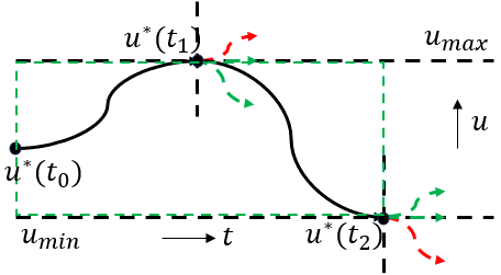
Figure 1: An illustration of how a predefined $\lambda$ affects the feasible region of a single control input under constraints (10c) and (20). The area of the green dashed rectangle denotes the maximum feasible region in which the controller can be selected to satisfy an additional constraint (10a). The black solid line denotes a continuous safe controller for $[t_{0},t_{2}].$ The green dashed arrows denote other possible control strategies under constraints (10c), (10a) and (20) with different $\lambda.$

VI Case Study and Simulations

In this section, we consider the Adaptive Cruise Control (ACC) problem for a heterogeneous platoon (3 vehicles), which is more realistic than the SACC problem introduced in Sec. IV and case study introduced in [8], [23].

VI-A Vehicle Dynamics

We consider a nonlinear vehicle dynamics in the form

$$\underbrace{\begin{bmatrix}\dot{x}_{j}(t)\\ \dot{v}_{j}(t)\end{bmatrix}}_{\dot{\bm{x}}_{j}(t)}=\underbrace{\begin{bmatrix}v_{j}(t)\\ -\frac{1}{M_{j}}F_{r}(v_{j}(t))\end{bmatrix}}_{f(\bm{x}_{j}(t))}+\underbrace{\begin{bmatrix}0\\ \frac{1}{M_{j}}\end{bmatrix}}_{g(\bm{x}_{j}(t))}u_{j}(t),$$ (26)

where $M_{j}$ denotes the mass of the $j^{th}$ vehicle, $j=1,2,3$ and $F_{r}(v_{j}(t))=f_{0}sgn(v_{j}(t))+f_{1}v_{j}(t)+f_{2}v^{2}_{j}(t)$ is the resistance force as in [26]; $f_{0},f_{1},f_{2}$ are positive scalars determined empirically and $v_{j}(t)>0$ denotes the velocity of the vehicle; $x_{j}(t),u_{j}(t)$ denote the position and acceleration of the vehicle, respectively. The first term in $F_{r}(t)$ denotes the Coulomb friction force, the second term denotes the viscous friction force and the last term denotes the aerodynamic drag.

VI-B Vehicle Limitations

Vehicle limitations include vehicle constraints on safe distance, speed and acceleration. We consider 3 vehicles driving along the same direction in a line. The first vehicle leads the second vehicle and the second vehicle leads the third vehicle.

Safe Distance Constraint: The distance is considered safe if $x_{j-1}(t)-x_{j}(t)>l_{p},j=2,3$ is satisfied $\forall t\in[0,T]$, where $l_{p}$ denotes the minimum distance two vehicles should maintain, and $j$ is the index of the second and third vehicles.

Speed Constraint: The second and third vehicles should achieve a desired speed $v_{j,d}>0$, $j=2,3$, respectively.

Acceleration Constraint: The second and third vehicles should minimize the following cost

$$\min_{u_{j}(t)}\int_{0}^{T}(\frac{u_{j}(t)-F_{r}(v_{j}(t))}{M_{j}})^{2}dt$$ (27)

when the acceleration is constrained in the form

$$-c_{j,d}M_{j}g\leq u_{j}(t)\leq c_{j,a}M_{j}g,\forall t\in[0,T],$$ (28)

where $g$ denotes the gravity constant, $c_{j,d}>0$ and $c_{j,a}>0$ are deceleration and acceleration coefficients respectively, $j=2,3.$

Problem 2.

Determine the optimal controllers for the second and third vehicles governed by dynamics (26), subject to the vehicle constraints on safe distance, speed and acceleration.

We consider a decentralized optimal control framework for the platoon, i.e., the kinematic information of the lead vehicle is generated by solving Prob. 2 and assumed to be known by the following vehicle. Since there is no vehicle leading the first vehicle, we define the controller for the first vehicle as

$$u_{1}(t)=2M_{1}\sin(2\pi t)+F_{r}(v_{1}(t)),$$ (29)

which represents the swift change of control strategy of the first vehicle. To satisfy the constraint on speed, we define a CLF $V_{j}(\bm{x}(t))\coloneqq(v_{j}(t)-v_{j,d})^{2}$ with $c_{j,1}=c_{j,2}=1$ to stabilize $v_{j}(t)$ to $v_{j,d}$ and formulate the relaxed constraint in (6) as

$$L_{f}V_{j}(\bm{x}_{j}(t))+L_{g}V_{j}(\bm{x}_{j}(t))u_{j}(t)+c_{j,3}V_{j}(\bm{x}_{j}(t))\leq\delta_{j}(t),$$ (30)

where $\delta_{j}(t)$ is a relaxation that makes (30) a soft constraint.

To satisfy the constraints on safety distance and acceleration, we define a continuous function $b_{j}(\bm{x}_{j}(t))=x_{j-1}(t)-x_{j}(t)-l_{p}$ as a HOCBF to guarantee $b_{j}(\bm{x}_{j}(t))\geq 0$ and constraint (28). To ensure there exists at least one solution to the optimization Prob. 2, we define a continuous function $b_{j,F}(\bm{x}_{j}(t))\geq 0$ to guarantee feasibility, and then formulate all constraints mentioned above into QPs to get the optimal controller. The parameters are $v_{1}(0)=13.89m/s,v_{2}(0)=8m/s,v_{3}(0)=14m/s,v_{2,d}=24m/s,v_{3,d}=25m/s,M_{1}=1500kg,M_{2}=1650kg,M_{3}=1550kg,g=9.81m/s^{2},x_{1}(0)=0m,x_{2}(0)=-100m,x_{3}(0)=-190m,l_{p}=10m,f_{0}=0.1N,f_{1}=5Ns/m,f_{2}=0.25Ns^{2}/m,c_{2,a}=0.4,c_{3,a}=0.35.$

VI-C Implementation with Auxiliary-Function Based CBFs

Let $b_{j}(\bm{x}_{j}(t))=x_{j-1}(t)-x_{j}(t)-l_{p}$. The relative degree of $b_{j}(\bm{x}_{j}(t))$ with respect to dynamics (26) is 2. The HOCBFs are then defined as

$$\begin{split}&\psi_{j,0}(\bm{x}_{j})\coloneqq b_{j}(\bm{x}_{j}),\\ &\psi_{j,1}(\bm{x}_{j})\coloneqq L_{f}b_{j}(\bm{x}_{j})+k_{j,1}b_{j}(\bm{x}_{j}),\\ &\psi_{j,2}(\bm{x}_{j},\bm{u}_{j})\coloneqq L_{f}^{2}b_{j}(\bm{x}_{j})+L_{f}L_{g}b_{j}(\bm{x}_{j})u_{j}+\\ &k_{j,1}L_{f}b_{j}(\bm{x}_{j})+k_{j,2}\psi_{j,1}(\bm{x}_{j}),\end{split}$$ (31)

where $\alpha_{j,1}(\cdot),\alpha_{j,2}(\cdot)$ are set as linear functions. We define $\varphi_{j,0}(\bm{x}_{j},\bm{a}_{j})\coloneqq\mathcal{A}_{j}(a_{j})b_{j,F}(\bm{x}_{j})>0$ as the modified feasibility constraint from (18), $\psi_{j,F}(\bm{x}_{j},\bm{u}_{j},\bm{a}_{j},\dot{\bm{a}}_{j})\geq\epsilon_{j}$ from (20) and $\mathcal{A}_{j}(a_{j})=e^{a_{j}}.$ The auxiliary-function based CBFs are defined as

$$\begin{split}&\varphi_{j,0}(\bm{x}_{j},\bm{a}_{j})\coloneqq e^{a_{j}}(L_{f}^{2}b_{j}(\bm{x}_{j})+\\ &[L_{f}L_{g}b_{j}(\bm{x}_{j})u_{j}]_{max}+k_{j,1}L_{f}b_{j}(\bm{x}_{j})+k_{j,2}\psi_{j,1}(\bm{x}_{j})),\\ &\psi_{j,F}(\bm{x}_{j},\bm{u}_{j},\bm{a}_{j},\dot{\bm{a}}_{j})\coloneqq\dot{\varphi}_{j,0}(\bm{x}_{j},\bm{u}_{j},\bm{a}_{j},\dot{\bm{a}}_{j})+l_{j,F}\varphi_{j,0}(\bm{x}_{j},\bm{a}_{j}),\\ \end{split}$$ (32)

where $\dot{a}_{j}=-\frac{(L_{f}b_{j,F}(\bm{x}_{j})+[L_{g}b_{j,F}(\bm{x}_{j})u_{j}]_{min})}{b_{j,F}(\bm{x}_{j})}.$ $\alpha_{j,F}(\cdot)$ is defined as a linear function. The derivative of the resistance force for two vehicles makes the equation of $\psi_{j,F}$ complicated and calls for the introduction of auxiliary adaptive $\dot{a}_{j}$. By formulating the constraints from HOCBFs (31), auxiliary-function based CBFs (32), CLF (30) and acceleration (28), we can define the cost function for the QP as

$$\begin{split}\min_{u_{j}(t),\delta_{j}(t)}\int_{0}^{T}[(\frac{u_{j}(t)-F_{r}(v_{j}(t))}{M_{j}})^{2}+p_{j}\delta_{j}(t)^{2}]dt.\end{split}$$ (33)

The remaining parameters are set as $a_{1}(0)=a_{2}(0)=1,c_{2,3}=c_{3,3}=1,p_{2}=p_{3}=1000,\epsilon_{2}=\epsilon_{3}=10^{-10}.$

VI-D Implementation with HOCBFs without Feasibility Constraint

As a benchmark, we consider the “traditional” optimization problem without the feasibility constraint formulated without the auxiliary-function based CBFs (32). In other words, the cost function is (33) and the constraints come from HOCBFs (31), CLF (30), and acceleration (28). All the corresponding parameters are set to the same values as above.

VI-E Simulation Results

In this subsection, we show how our proposed auxiliary-function based CBF method guarantees feasibility and safety and outperforms the benchmark described above, which does not use the feasibility constraint.

We consider Prob. 2 with different control bounds (28) (due to smoothness of vehicle tires and road surfaces), and implement HOCBFs as safety constraints with or without feasibility constraint for solving Prob. 2 in MATLAB. We use ode45 to integrate the dynamics for every $0.1s$ time-interval and quadprog to solve the QPs. The proposed method shows varying degrees of adaptivity to different lower control bounds in terms of feasibility, safety and optimality.

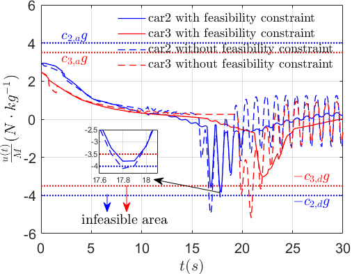
(a) Acceleration of the $2^{nd},3^{rd}$ vehicles vs. time.

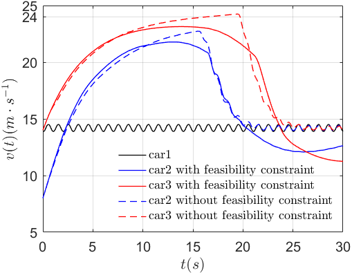
(b) Velocity of the $1^{st},2^{nd},3^{rd}$ vehicles vs. time.

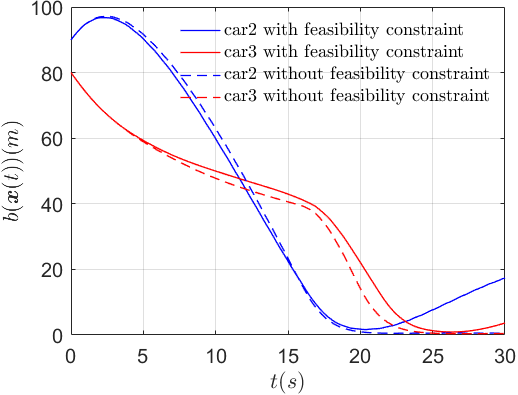
(c) $b(\bm{x})$ of the $2^{nd},3^{rd}$ vehicles vs. time.

Figure 2: Case 1-Feasibility constraint enhances feasibility for solving Prob. 2. The hyperparameters are set as $k_{2,1}=k_{2,2}=k_{3,1}=k_{3,2}=1,l_{2,F}=l_{3,F}=0.1.$ The lower control bounds are $c_{2,d}=0.4,c_{3,d}=0.35.$ Note that without feasibility constraint, the deceleration of the $2^{nd}$(blue), $3^{rd}$(red) vehicles exceeds deceleration bound, therefore the control bounds are violated (as shown by dashed lines in (a)), which causes infeasibility even though the safety is satisfied as shown in (c).

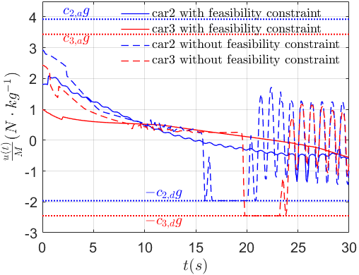
(a) Acceleration of the $2^{nd},3^{rd}$ vehicles vs. time.

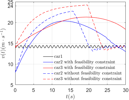
(b) Velocity of the $1^{st},2^{nd},3^{rd}$ vehicles vs. time.

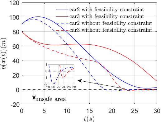
(c) $b(\bm{x})$ of the $2^{nd},3^{rd}$ vehicles vs. time.

Figure 3: Case 2-Feasibility constraint enhances safety for solving Prob. 2. The hyperparameters are set as $k_{2,1}=k_{2,2}=k_{3,1}=k_{3,2}=1,l_{2,F}=l_{3,F}=0.05.$ The lower control bounds are $c_{2,d}=0.2,c_{3,d}=0.25$ (tighter than Fig. 2). Note that without feasibility constraint, the $b(\bm{x})$ of the $2^{nd}$(blue), $3^{rd}$(red) vehicles exceeds safety bound, therefore the safe distance between vehicles can be negative (as shown by dashed lines in (c)), which causes danger even though the control bounds are satisfied as shown in (a).

We compare two CBF-based methods in terms of the feasibility of the corresponding QPs. The only difference between the two methods is that one method additionally uses our proposed auxiliary-function based CBFs to enforce feasibility constraint, while another one is without feasibility constraint. In Fig. 2, we keep hyperparameters of safety related HOCBFs the same for two methods as $k_{2,1}=k_{2,2}=k_{3,1}=k_{3,2}=1.$ Two extra hyperparameters are set as $l_{2,F}=l_{3,F}=0.1$ for the feasibility constraint related CBFs. The lower control bounds for two vehicles are: $-c_{2,d}M_{2}g,-c_{3,d}M_{3}g$ where $c_{2,d}=0.4,c_{3,d}=0.35.$ In Fig. 2(a), it shows that solving QPs for the second and third vehicles is always feasible (denoted by solid lines) with the feasibility constraint since the acceleration is always within bounds while the QPs will become infeasible (denoted by dashed lines, starting from $t=16.7s,17.8s,19.9s,20.7s,21.8s.$) without this constraint since the deceleration of two vehicles exceed deceleration bound. The reason of the effectiveness of the feasibility constraint can be found in Fig. 2(b). With feasibility constraint, the vehicle tends to brake earlier, therefore reaches a smaller peak velocity to avoid a delayed steep deceleration. Since $b(\bm{x})\geq 0,$ the safe distance $l_{p}$ is always maintained for two vehicles $\forall t\in[0,30s],$ which can be seen in Fig. 2(c) and shows the safety is always guaranteed for two methods.

To test the adaptivity to tighter deceleration bound for two methods, we set the lower control bounds $-c_{2,d}M_{2}g,-c_{3,d}M_{3}g$ for two vehicles with $c_{2,d}=0.2,c_{3,d}=0.25.$ In this case we compare two CBFs based methods in terms of safety, without caring about the feasibility. The only difference between two methods is one method additionally uses our proposed auxiliary-function based CBFs to enforce feasibility constraint while another one without feasibility constraint makes vehicles brake at the maximum deceleration when vehicle’s deceleration is about to exceed its bound. In Fig. 3, we keep hyperparameters of safety related HOCBFs the same for two methods as $k_{2,1}=k_{2,2}=k_{3,1}=k_{3,2}=1.$ Two extra hyperparameters are set as $l_{2,F}=l_{3,F}=0.05$ for the feasibility constraint related CBFs. Even both methods satisfy the acceleration constraint as shown in Fig. 3(a), our proposed method shows more effectiveness on maintaining safe distance between two vehicles (denoted by solid lines). Without feasibility constraint, two vehicles can not maintain the safe distance $l_{p}$ since $b(\bm{x})<0$ (denoted by dashed lines, starting from $t=18.7s,22.9s$), which is illustrated in Fig. 3(c). The reason can be explained in Fig. 3(b) that the feasibility constraint helps two vehicles to brake earlier, therefore two vehicles can maintain a longer distance from the corresponding lead vehicle.

We also notice that due to control strategy (29) used for the first vehicle, the velocity curves in Fig. 2(b) and 3(b) vibrate frequently (denoted by solid black curve), which might cause the sharp transition of control in the middle shown by dashed curves in Fig. 2(a) and 3(a). Compared to this, our proposed method can generate a smoother optimal controller denoted by solid curves, which might make contribution to reducing more energy cost (increasing optimality).

VII Conclusion and Future Work

We propose auxiliary-function based CBFs as sufficient constraints for safety and feasibility guarantees of constrained optimal control problems, which work for general affine control systems. We have demonstrated the effectiveness of our proposed method in this paper by applying it to an adaptive cruise control problem for a heterogeneous platoon. There are still some scenarios the current method can not perfectly handle, i.e., many other hard constraints are added to optimization problems due to requirements beyond safety, which may lead to conflicts between various constraints. We will address this limitation in future work by creating a more general CBFs-based method with less conservative conditions for constrained optimal control problems.

References

- [1] K. P. Tee, S. S. Ge, and E. H. Tay, “Barrier lyapunov functions for the control of output-constrained nonlinear systems,” Automatica, vol. 45, no. 4, pp. 918–927, 2009.
- [2] S. Boyd, S. P. Boyd, and L. Vandenberghe, Convex optimization. Cambridge university press, 2004.
- [3] J.-P. Aubin, A. M. Bayen, and P. Saint-Pierre, Viability theory: new directions. Springer Science & Business Media, 2011.
- [4] S. Prajna, A. Jadbabaie, and G. J. Pappas, “A framework for worst-case and stochastic safety verification using barrier certificates,” IEEE Transactions on Automatic Control, vol. 52, no. 8, pp. 1415–1428, 2007.
- [5] D. Panagou, D. M. Stipanovič, and P. G. Voulgaris, “Multi-objective control for multi-agent systems using lyapunov-like barrier functions,” in 52nd IEEE Conference on Decision and Control, 2013, pp. 1478–1483.
- [6] L. Wang, A. D. Ames, and M. Egerstedt, “Multi-objective compositions for collision-free connectivity maintenance in teams of mobile robots,” in 2016 IEEE 55th Conference on Decision and Control (CDC), 2016, pp. 2659–2664.
- [7] P. Glotfelter, J. Cortés, and M. Egerstedt, “Nonsmooth barrier functions with applications to multi-robot systems,” IEEE control systems letters, vol. 1, no. 2, pp. 310–315, 2017.
- [8] A. D. Ames, X. Xu, J. W. Grizzle, and P. Tabuada, “Control barrier function based quadratic programs for safety critical systems,” IEEE Transactions on Automatic Control, vol. 62, no. 8, pp. 3861–3876, 2016.
- [9] A. D. Ames, K. Galloway, and J. W. Grizzle, “Control lyapunov functions and hybrid zero dynamics,” in 2012 IEEE 51st IEEE Conference on Decision and Control (CDC), 2012, pp. 6837–6842.
- [10] Q. Nguyen and K. Sreenath, “Exponential control barrier functions for enforcing high relative-degree safety-critical constraints,” in 2016 American Control Conference (ACC), 2016, pp. 322–328.
- [11] W. Xiao and C. Belta, “High-order control barrier functions,” IEEE Transactions on Automatic Control, vol. 67, no. 7, pp. 3655–3662, 2021.
- [12] A. Isaly, B. C. Allen, R. G. Sanfelice, and W. E. Dixon, “Zeroing control barrier functions for safe volitional pedaling in a motorized cycle,” IFAC-PapersOnLine, vol. 53, no. 5, pp. 218–223, 2020.
- [13] C. Khazoom, D. Gonzalez-Diaz, Y. Ding, and S. Kim, “Humanoid self-collision avoidance using whole-body control with control barrier functions,” in 2022 IEEE-RAS 21st International Conference on Humanoid Robots (Humanoids), 2022, pp. 558–565.
- [14] M. Cavorsi, B. Capelli, L. Sabattini, and S. Gil, “Multi-robot adversarial resilience using control barrier functions,” in Robotics: Science and Systems, 2022.
- [15] J. Zeng, B. Zhang, and K. Sreenath, “Safety-critical model predictive control with discrete-time control barrier function,” in 2021 American Control Conference (ACC), 2021, pp. 3882–3889.
- [16] S. Liu, J. Zeng, K. Sreenath, and C. A. Belta, “Iterative convex optimization for model predictive control with discrete-time high-order control barrier functions,” in 2023 American Control Conference (ACC), 2023, pp. 3368–3375.
- [17] T. Gurriet, M. Mote, A. D. Ames, and E. Feron, “An online approach to active set invariance,” in 2018 IEEE Conference on Decision and Control (CDC), 2018, pp. 3592–3599.
- [18] A. Singletary, P. Nilsson, T. Gurriet, and A. D. Ames, “Online active safety for robotic manipulators,” in 2019 IEEE/RSJ International Conference on Intelligent Robots and Systems (IROS), 2019, pp. 173–178.
- [19] T. Gurriet, M. Mote, A. Singletary, P. Nilsson, E. Feron, and A. D. Ames, “A scalable safety critical control framework for nonlinear systems,” IEEE Access, vol. 8, pp. 187 249–187 275, 2020.
- [20] Y. Chen, M. Jankovic, M. Santillo, and A. D. Ames, “Backup control barrier functions: Formulation and comparative study,” in 2021 60th IEEE Conference on Decision and Control (CDC), 2021, pp. 6835–6841.
- [21] E. Squires, P. Pierpaoli, and M. Egerstedt, “Constructive barrier certificates with applications to fixed-wing aircraft collision avoidance,” in 2018 IEEE Conference on Control Technology and Applications (CCTA), 2018, pp. 1656–1661.
- [22] J. Breeden and D. Panagou, “High relative degree control barrier functions under input constraints,” in 2021 60th IEEE Conference on Decision and Control (CDC), 2021, pp. 6119–6124.
- [23] W. Xiao, C. Belta, and C. G. Cassandras, “Adaptive control barrier functions,” IEEE Transactions on Automatic Control, vol. 67, no. 5, pp. 2267–2281, 2021.
- [24] S. Liu, W. Xiao, and C. A. Belta, “Auxiliary-adaptive control barrier functions for safety critical systems,” arXiv preprint arXiv:2304.00372, 2023.
- [25] W. Xiao, C. A. Belta, and C. G. Cassandras, “Sufficient conditions for feasibility of optimal control problems using control barrier functions,” Automatica, vol. 135, p. 109960, 2022.
- [26] H. K. Khalil, Nonlinear systems; 3rd ed. Upper Saddle River, NJ: Prentice-Hall, 2002, the book can be consulted by contacting: PH-AID: Wallet, Lionel. [Online]. Available: https://cds.cern.ch/record/1173048
- [27] K. Xu, W. Xiao, and C. G. Cassandras, “Feasibility guaranteed traffic merging control using control barrier functions,” in 2022 American Control Conference (ACC). IEEE, 2022, pp. 2309–2314.
- [28] J. Zeng, B. Zhang, Z. Li, and K. Sreenath, “Safety-critical control using optimal-decay control barrier function with guaranteed point-wise feasibility,” in 2021 American Control Conference (ACC), 2021, pp. 3856–3863.