CausalImages: An R Package for Causal Inference with Earth Observation, Bio-medical, and Social Science Images

Connor T. Jerzak, Adel Daoud CausalImages: An R Package for Causal Inference with Earth Observation, Bio-medical, and Social Science Images CausalImages: A Package for Causal Inference with Images The causalimages R package enables causal inference with image and image sequence data, providing new tools for integrating novel data sources like satellite and bio-medical imagery into the study of cause and effect. One set of functions enables image-based causal inference analyses. For example, one key function decomposes treatment effect heterogeneity by images using an interpretable Bayesian framework. This allows for determining which types of images or image sequences are most responsive to interventions. A second modeling function allows researchers to control for confounding using images. The package also allows investigators to produce embeddings that serve as vector summaries of the image or video content. Finally, infrastructural functions are also provided, such as tools for writing large-scale image and image sequence data as sequentialized byte strings for more rapid image analysis. causalimages therefore opens new capabilities for causal inference in R, letting researchers use informative imagery in substantive analyses in a fast and accessible manner.
Repository: GitHub.com/AIandGlobalDevelopmentLab/causalimages-software Causal inference, image analysis, image-sequence data, computer vision, machine learning, R Causal inference, image data, image sequence data, computer vision, machine learning, R Connor T. Jerzak
Department of Government
University of Texas at Austin
110 Inner Campus Drive
Austin, TX 78712
E-mail:
URL: ConnorJerzak.com

Adel Daoud
Institute for Analytical Sociology
Linköping University
SE-581 83 Linköping Sweden
E-mail:
URL: AdelDaoud.se

1 Introduction: Causal Inference with Images

Satellite image data represents an emerging resource for research in global development and earth observation, yet no R package currently exists to handle images for causal inference up to now. By causal inference, we refer to the rich literature in statistics (Imbens and Rubin, 2016), computer science (Pearl, 2009), and beyond (Hernan and Robins, 2020). Satellites generate temporally-rich worldwide coverage, capturing the entire Earth’s surface at regular intervals, except when obscured by clouds (Burke et al., 2021). Historical archives date back to the 1970s. Unlike snapshots of political, economic, or educational systems at a single time point, satellites revisit each location every 2 weeks or more, providing approximately 26 temporal observations annually. This time-series information has proven valuable for studying phenomena like transportation network growth (Nagne and Gawali, 2013), urbanization (Schneider et al., 2009), health and living conditions (Daoud et al., 2023; Chi et al., 2022), living standards (Yeh et al., 2020; Pettersson et al., 2023), and neighborhood characteristics (Sowmya and Trinder, 2000). Thus, satellite data facilitates observational inference where ground-level data is lacking. Moreover, image quality and frequency continue improving as the satellite population proliferates from hundreds to thousands (Tatem et al., 2008), with sub-100 cm resolution now available (Hallas, 2019). We see an example of this data source in Figure 1.

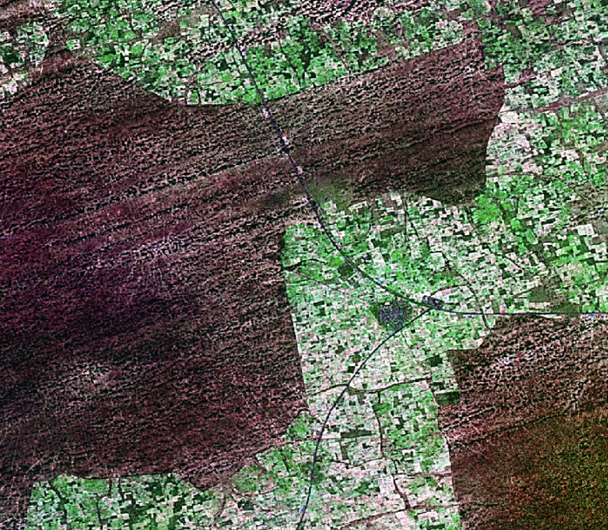
Figure 1: Landsat satellite imagery over Nigeria.

Methodological guidance has remained limited for causal estimation from satellite images (Daoud and Dubhashi, 2023). To address that methodological gap, recently Jerzak et al. (2022) proposed methods to estimate confounding, and Jerzak et al. (2023) developed methods for estimating effect heterogeneity in images. Our causalimages package encompasses these methods and some future ones. Our confounding method helps address that research need by examining observational causal inference amidst image-based confounding. Our heterogeneity method shows how researchers may use past satellite images to proxy geographical and historical processes important for moderating the treatment effect of both randomized experiments and observational studies.

Our causal inference work with images complements the growing use of visual data in climate science, sociology, economics, political science, and biomedical research (Kino et al., 2021; Daoud and Dubhashi, 2023). Examples include qualitative photo analysis (Pauwels, 2010; O’Hara and Higgins, 2019), image similarity calculation (Zhang and Peng, 2022), crowd size estimation (Cruz and González-Villa, 2021), and relating social outcomes to Street View scenes (Gebru et al., 2017). Recent extensions encompass video for investigating social processes like police violence (Nassauer and Legewie, 2021). In large-data quantitative studies, algorithms have been trained to identify objects of interest automatically (Torres and Cantú, 2022). Similarly, in the biomedical domain, Castro et al. (2020) shows how a variety of image data—from X-ray to ultrasound pictures to MRI scans—can be used for causal inference. However, more research is needed to close the gap between foundational and applied research across those domains, and not only earth observation data. To contribute to closing that gap, we created causalimages. Although our examples focus on satellite images, research can use any image data and across other domains where image data are available.

In concluding this introduction, we note that this package builds on the R ecosystem regarding data visualization and geospatial analysis. For instance, the R packages like tensorflow and keras provide the backbone for deep learning functionalities with the TensorFlow backend. The viridis package enhances the visualization capabilities, while animation facilitates dynamic plots for results involving image sequence data. Integration with Python is streamlined through reticulate. For geospatial operations, we rely on geosphere and raster.

2 Models and Software

2.1 Package Overview

At a high level, the causalimages package provides tools for causal inference with image data. The package contains several functions whose relations are summarized in Figure 2.

The AnalyzeImageConfounding and AnalyzeImageHeterogeneity, functions run the main analysis models for image causality. They require observed treatment and outcome data, as well as a way to retrieve image data associated with each observation.

Other functions center on working with image data in a more infrastructural sense. The GetAndSaveGeolocatedImages function helps retrieve image data referenced by geographic coordinates. WriteTfRecord writes image or image sequence data to a sequentialized TFRecord file for efficient retrieval. GetImageEmbeddings generates embeddings useful for other tasks where an efficient summary of the image information is required.

Figure 2: Overview of workflow in the causalimages package.

Together, these tools enable causal analyses that incorporate image data as confounders, mediators, and moderators of treatment effects. The analyses can adjust for spatial dependencies and estimate heterogeneous treatment effects associated with geospatial imagery.

2.2 Package Installation and Loading

The causalimages package is currently installed using the devtools package. For installation, users should run: R> devtools::install_github(repo = "AIandGlobalDevelopmentLab/causalimages-software") To load the package into a live R environment, use: R> library(causalimages)

The causalimages package uses a tensorflow backend for image analysis and GPU utilization. Python version 3 or above is assumed. To install tensorflow into your default Python environment, try R> library(reticulate) R> py_install("tensorflow") You may need to do the same to install dependencies such as tensorflow-probability and gc. For more fine-grained user control over CPU and GPU use, we recommend installing the requisite backend into a conda environment.

2.3 Tutorial Data

Once the package has been successfully initiated, users can access package data useful for tutorial purposes. The data are drawn from an anti-poverty experiment in Uganda Blattman et al. (2020) and contain information on the treatment, experimental outcome, approximate coordinates for each unit, as well as pre-treatment covariates and geo-referenced satellite images for each unit. To allow researchers to load all images into memory, we have cropped these images to a smaller-than-original size. R> data(CausalImagesTutorialData) The Blattman data are then structured as follows: R> summary(obsW) R> summary(obsY) R> summary(LongLat) R> summary(X) R> causalimages::image2(FullImageArray[1,,,1]) # image associated with unit 1 R> causalimages::image2(FullImageArray[3,,,2]) # image associated with unit 3

2.4 Functions for Data Assimilation

We have several functions for helping users save geo-located images. For example, GetAndSaveGeolocatedImages finds the image slice associated with given longitude and latitude values and saves images by band, given a pool of .tif’s. For example, the .tif pool may contain dozens of large Landsat mosaics covering the continent of Africa, and we want to extract a 500$\times$500 meter square image around a particular point. For the Blattman data, we have provided the Landsat images in the package. For other data, the user has to download data from USGS or Google Earth Engine.

In the following example, we have two .tif’s saved in "./LargeTifs", we can search across those images for matches to the associated long and lat inputs. When a match is found, a series of .csv’s are written to encompass the data in a image_pixel_width square around the target geo-point in the target .tif. These image objects are saved in the save_folder as Key[key]_BAND[band].csv where [key] refers to the appropriate entry from keys specifying the label for each image and [band] specifies the band. R> MASTER_IMAGE_POOL_FULL_DIR <- c("./LargeTifs/tif1.tif","./LargeTifs/tif2.tif") R> GetAndSaveGeolocatedImages( + long = GeoKeyMat$geo_{l}ong,+lat=GeoKeyMat$geo_lat, + image_pixel_width = 500L, + keys = row.names(GeoKeyMat), + tif_pool = MASTER_IMAGE_POOL_FULL_DIR, + save_folder = "./Data/Uganda2000_processed", + save_as = "csv", + lyrs = NULL)

2.5 Functional Image Loading

One important part of the image analysis pipeline is writing a function that acquires the appropriate image data for each observation. This function will be fed into the acquireImageFxn argument of the package functions unless an approach using TFRecords is used instead. There are two ways that you can approach this: (1) you may store all images in R’s memory (feasible only for problems involving few or small images), or you may (2) save images on your hard drive (e.g., using GetAndSaveGeolocatedImages) and read them in when needed. The second option will be more common for large images.

You will write your acquireImageFxn to take in one main argument—keys. keys is fed a character or numeric vector. Each value of keys refers to a unique image object that will be read in. If each observation has a unique image associated with it, perhaps imageKeysOfUnits = 1:nObs. If multiple observations map to the same image, then multiple observations will map to the same keys value. The keys thus serves as an identifier for a particular image, which is then referenced back to individuals who are matched with keys of their associated image.

In practice, users should ensure that acquireImageFxn returns arrays with dimensions batch by height by width by channels in the case of images and batch by time by height by width by channels in the case of image sequences/videos.

2.5.1 When Loading All Images in Memory

We here provide an example of writing an acquireImageFxn function using the tutorial data wherein the images are already read into memory. R> acquireImageFromMemory <- function(keys, training = F) + m_<- FullImageArray[match(keys, KeysOfImages),,,] + if(length(keys) == 1) + m_<- array(m_,dim = c(1L,dim(m_)[1],dim(m_)[2],dim(m_)[3])) + + return( m_) +

To run this acquireImageFunction in practice, we would take R> ImageSet <- acquireImageFromMemory(KeysOfObservations[c(5,7)]) where ImageSet contains the images associated with observations 5 and 7 (note that they could both have the same image if these units are co-located).

2.5.2 When Reading in Images from Disk

For most applications of large-scale causal image analysis, we won’t be able to read the whole set of images into R’s memory. Instead, we can specify a function that will read images from somewhere on your hard drive. You can also experiment with other methods—as long as you can specify a function that returns an image when given the appropriate imageKeysOfUnits value, you should be fine. Here’s an example of an acquireImageFxn that reads images from disk:

R> acquireImageFromDisk <- function(keys, training = F) + array_shell <- array(NA,dim = c(1L,imageHeight,imageWidth,NBANDS)) + array_<- sapply(keys,function(key_) + for(band_in 1:NBANDS) + array_shell[,,,band_] <- + (as.matrix(data.table::fread( + input = sprintf("./Data/Uganda2000_processed/Keykey_, band_),header = F)[-1,] )) + + return( array_shell ) + , simplify="array") + array_<- tf$squeeze(tf$constant(array_,dtype=tf$float32),0L)+array_{<}-tf$transpose(array_,c(3L,0L,1L,2L)) + return( array_) +

2.6 TFRecords Integration for Fast Image Processing

We can use the aforementioned functions for acquiring images from disk to write the data corpus in an optimized format for fast reading-writing. This format is not required but is highly recommended to improve causal image analysis runtimes.

In particular, once we have acquired a pool of geo-referenced satellite images, causalimages also contains a function that writes the analysis data in TFRecord format, a binary storage format used by TensorFlow to store data efficiently and to enable fast acquisition of data into memory in serialized chunking—a process that speeds up the acquisition of images into memory where data are too large to fit into memory. R> WriteTfRecord( + file = "./UgandaApp.tfrecord", + keys = KeysOfObservations, + acquireImageFxn = acquireImageFromMemory, + conda_env = "tensorflow_m1") WriteTfRecord writes to TFRecords format the entire image data stream. As we discuss later, this same function can be used if the inputted acquireImageFxn function outputs image sequences.

2.7 Image and Image Sequence Embeddings

The GetImageEmbeddings function offers a methodology for the extraction of image and video embeddings, particularly tailored for earth observation tasks that drive causal inference. Using the randomized convolutions approach in Rolf et al. (2021), the function generates vector representations of images and image sequences based on the similarity within these data to a large set of smaller image patterns (i.e. kernels). The parameters provided to the function allow fine-tuned control over the embedding process, especially in the kind of convolutional kernels used. This flexibility can allow the embeddings to be adapted for the given dataset.

We note that the embeddings function works with both image and image sequence data. It can also be run in the de-confounding and heterogeneity decomposition functions we will analyze later.

To use the function, you can specify how to load images via the acquireImageFxn R> MyImageEmbeddings <- GetImageEmbeddings( + imageKeysOfUnits = KeysOfObservations[ take_indices ], + acquireImageFxn = acquireImageFromMemory, + nEmbedDim = 100, + kernelSize = 3L, + conda_env = "tensorflow_m1", + conda_env_required = T ) Again, conda_env specifies a conda environment in which the desired version of the TensorFlow backend lives. If NULL, we search in the default Python environment for the backend.

Alternatively, you may use the tfrecords approach as follows: R> MyImageEmbeddings <- GetImageEmbeddings( + file = "./UgandaApp.tfrecord", + nEmbedDim = 100, + kernelSize = 3L, + conda_env = "tensorflow_m1", + conda_env_required = T )

Finally, we can also obtain embeddings over image sequences. To do so, we first write a simple function creating image sequences given keys. R> acquireVideoRepFromMemory <- function(keys, training = F) + tmp <- acquireImageFromMemory(keys, training = training) + + if(length(keys) == 1) + tmp <- array(tmp,dim = c(1L,dim(tmp)[1],dim(tmp)[2],dim(tmp)[3])) + + + tmp <- array(tmp,dim = c(dim(tmp)[1], + 2, + dim(tmp)[3], + dim(tmp)[4], + 1L)) + return( tmp ) + To obtain video embeddings, we take: R> MyVideoEmbeddings <- GetImageEmbeddings( + imageKeysOfUnits = KeysOfObservations[ take_indices ], + acquireImageFxn = acquireVideoRepFromMemory, + temporalKernelSize = 2L, + kernelSize = 3L, + nEmbedDim = 100, + conda_env = "tensorflow_m1", + conda_env_required = T) We can also write a TFRecord and use that in obtaining image sequence embeddings by specifying the file argument.

2.8 Deconfounding with Image and Image Sequence

Using the AnalyzeImageConfounding function, causal effects are estimated using image-based or image-sequence-based confounders, although we add the option to include tabular confounders as well.

R> ImageConfoundingAnalysis <- AnalyzeImageConfounding( + obsW = obsW[ take_indices ], + obsY = obsY[ take_indices ], + X = X[ take_indices,apply(X[ take_indices,],2,sd)>0], + long = LongLat$geo_{l}ong[take_{i}ndices],+lat=LongLat$geo_lat[ take_indices ], + imageKeysOfUnits = KeysOfObservations[ take_indices ], + acquireImageFxn = acquireImageFromMemory, + batchSize = 4, + #modelClass = "cnn", # uses convolutional network (richer model class) + modelClass = "embeddings", # uses image embeddings (faster) + file = NULL, + plotBands = c(1,2,3), + dropoutRate = 0.1, + tagInFigures = T, figuresTag = "TutorialExample", + nBoot = 10, + nSGD = 10, # this should be more like 1000 in full analysis + figuresPath = " /Downloads", # figures saved here + conda_env = "tensorflow_m1", + conda_env_required = T +) AnalyzeImageConfounding returns a list containing an image-adjusted ATE estimate tauHat_propensityHajek (see Jerzak et al. (2022) for details) and an uncertainty estimate, tauHat_propensityHajek_se. A matrix of out-of-sample performance metrics (e.g., out-of-sample negative log-likelihood) is housed in ModelEvaluationMetrics. Users can specify whether they would like to use the faster option, modelClass = "embeddings", or the more computationally intensive but richer modeling approach using end-to-end convolutional neural network (CNN) training modelClass = "cnn". To speed up performance, we recommend letting acquireImageFxn = NULL and instead writing and then specifying a TFRecords file (e.g., set file to the path of the TFRecord saved via a call to WriteTfRecord).

In addition to providing these estimated quantities, the function also writes to disk summary PDF outputs containing salience maps, which quantify areas in the image or image sequence that, if changed, would lead to the largest change in predicted treatment probability. An example of such figures is found in Figure 3. Note that this figure can be made for either the embeddings or CNN image modeling backbone.

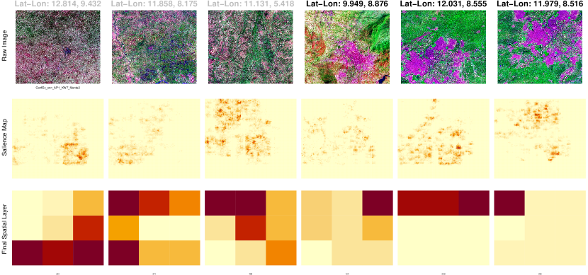
Figure 3: The three panels on the left illustrate the unprocessed data for control units, relevance diagrams for the predicted treatment likelihood, and the outcome from the concluding spatially detailed layer of the CNN image framework. The trio of panels on the right shows comparable elements for the treated units.

2.9 Heterogeneity Analysis with Image and Image Sequence Data

Using the AnalyzeImageHeterogeneity function, Conditional Average Treatment Effects (CATEs) are estimated using image-based or image-sequence-based pre-treatment information, although we add the option to include tabular pre-treatment covariates as well if the X argument is fed a numeric matrix input. This function would be used, for example, if we would want to learn about the kinds of geographies or developmental trajectories, proxied by satellite image data, most conducive to favorable responses to anti-poverty interventions. There are also possible applications in the biomedical domain where image data could be associated with a high or low response to a drug.

The functionality of AnalyzeImageHeterogeneity works much like AnalyzeImageConfounding:

R> ImageHeterogeneityResults <- AnalyzeImageHeterogeneity(
+    # data inputs
+    obsW =  UgandaDataProcessed$Wobs,
+    obsY = UgandaDataProcessed$Yobs,
+    imageKeysOfUnits =  UgandaDataProcessed$geo_long_lat_key,
+    acquireImageFxn = acquireImageFromDisk,
+    conda_env = "tensorflow_m1", # change to your conda env
+    conda_env_required = T,
+    X = X,
+    plotBands = 1L,
+    lat =  UgandaDataProcessed$geo_lat, # not required, deals with redundant locs
+    long =  UgandaDataProcessed$geo_long, # not required, deals with redundant locs
+
+    # inputs to control where visual results are saved as PDF or PNGs
+    plotResults = T,
+    figuresPath = "~/Downloads/",
+    printDiagnostics = T,
+    figuresTag = "causalimagesTutorial",
+
+    # optional arguments for generating transportability maps
+    transportabilityMat = NULL,
+
+    # other modeling options
+    modelClass = "embeddings", # uses image/video embeddings model class
+    orthogonalize = F,
+    heterogeneityModelType = "variational_minimal",
+    kClust_est = 2,
+    nMonte_variational = 2L,
+    nSGD = 4L,
+    batchSize = 34L,
+    kernelSize = 3L, maxPoolSize = 2L, strides = 2L,
+    nDepthHidden_conv = 2L,
+    nFilters = 64L,
+    nDepthHidden_dense = 0L,
+    nDenseWidth = 32L,
+    nDimLowerDimConv = 3L
+)

The function performs the image heterogeneity decomposition analysis delineated in Jerzak et al. (2023). Users specify the treatment variable and outcome data, alongside a specific function that guides the loading of images using reference keys for each unit, the function produces several outputs. All outputs are saved in a list. The clusterTaus_mean serves to present the estimated image effect cluster means, while the clusterTaus_sd contains the estimated standard deviations of those effect clusters.

The function further produces the clusterProbs_mean, which contains the average probabilities of these image effect clusters. Additionally, it offers an estimation of the standard deviations for these cluster probabilities through the clusterTaus_sd. For a deeper dive into the probabilistic insights, the clusterProbs_lowerConf gives the estimated lower confidence bounds for the effect cluster probabilities.

Regarding treatment effects, the function computes the impliedATE, a derived average treatment effect, and the individualTau_est, which highlights estimated treatment effects on an individual image basis. The transportabilityMat avails a matrix filled with cluster information, essential for analyses involving areas outside the original study locales. Lastly, to ensure data integrity, the whichNA_dropped output identifies those observations that were excluded because of missing values.

In addition to providing these estimated quantities, the function also writes to disk summary PDF outputs containing salience maps, which quantify areas in the image or image sequence that, if changed, would lead to the largest change in predicted treatment effect cluster probability. An example of such figures is found in Figure 4.

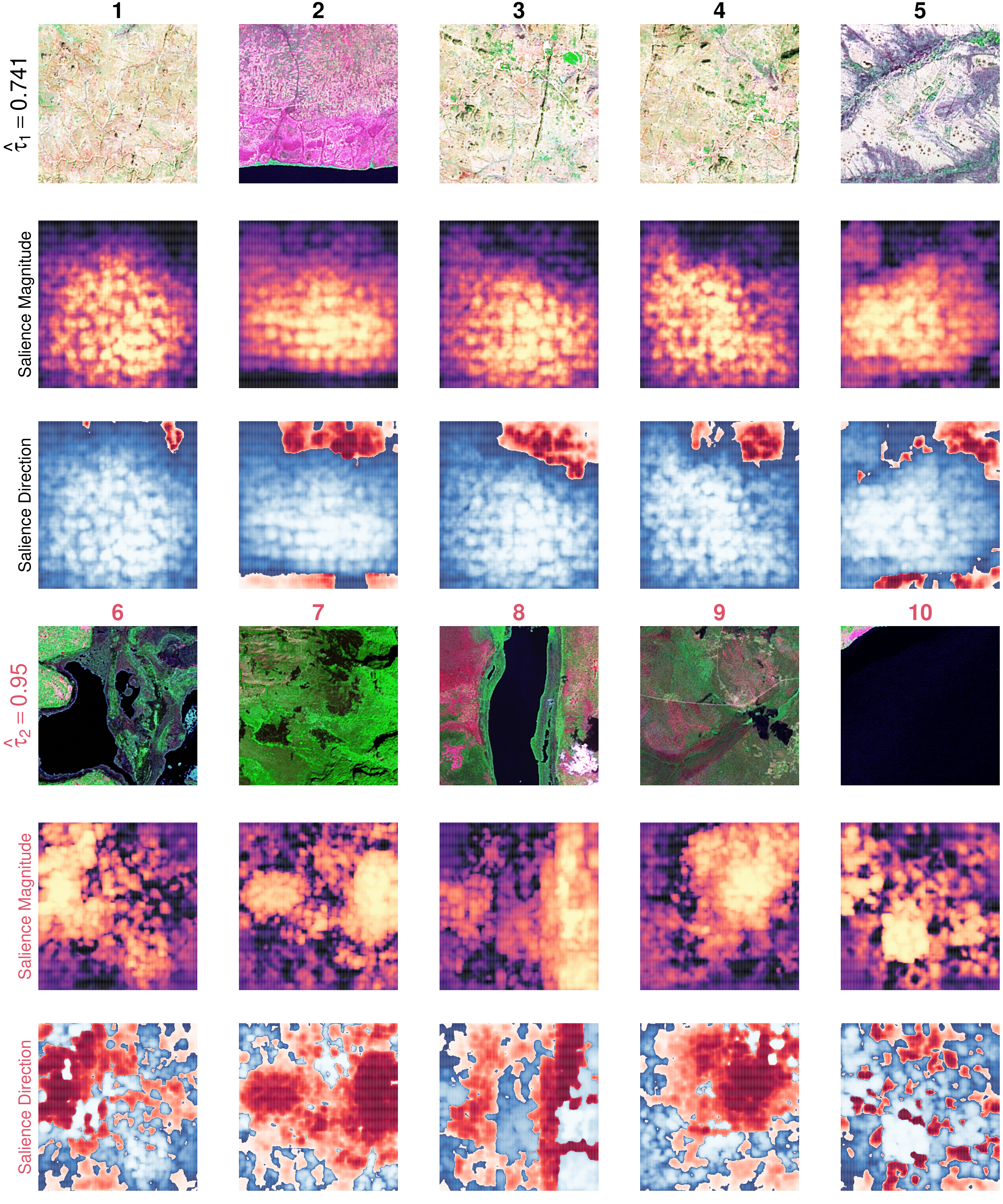
Figure 4: Left, top 3 rows: High probability cluster 1 images. Left, bottom 3 rows: High probability cluster 2 images. “Salience Magnitude” and “Direction” represent two ways of analyzing salience. See Jerzak et al. (2023) for details.

We note that the image (sequence) heterogeneity analysis can be made for either the embeddings or CNN image modeling backbone.

3 Conclusion and Future Development

As previously mentioned, causalimages closes the gap between foundational and applied research in using image data for causal inference (Jerzak et al., 2022, 2023). Besides the application cases discussed, we expect a take up in climate research, particularly pertaining to research in natural disaster evaluation (Shiba et al., 2021a, b; Kakooei et al., 2022; Daoud et al., 2016), armed conflict, and ecology. These research fields include processes occurring on the surface of the earth with often substantial impact that is measurable from space. In the age of data science, an increasing number of researchers are using image data (Daoud and Dubhashi, 2023). Although the package focuses on earth observation and global development research, the package is usable across a variety of domains in economics (Hall, 2010; Henderson et al., 2012), sociology (Daoud et al., 2023), public policy (Balgi et al., 2022), public health (Kino et al., 2021; Conklin et al., 2018), and biomedical applications (Castro et al., 2020).

Having discussed the current functionalities of causalimages, we now turn to the future development of it. We discuss four developments we will implement in the near future. First, we will modularize the image models that power causalimages, allowing the user to plug in their preferred image model or extend it with a different backbone (i.e., feature extractor). Currently, the causalimages uses two types of image-modeling backbones: the randomized embedding and the CNNs. While the CNN is a supervised procedure, the embedding backbone is unsupervised. However, there are many different foundational image-processing models or model architectures that the user might wish to consider using—VGGs, ResNets, U-NETs, LSTMS, Inception, and Transformers-based models.

These models allow the user to calibrate their modeling approach to the data at hand. Additionally, there are several pre-trained models trained on classical datasets such as ImageNEt or CIFAR, or earth observation data. For example, recently, NASA and IBM trained such a model (Fraccaro et al., 2023). Using these models in combination with the principles of transfer learning, will enable researchers to adapt their image models to often small datasets that we encounter in the biomedical and social sciences. Thus, modularization will enable the user to adapt causalimages for their data and modeling needs.

Second, we will create image simulation facilities for causal inference. Often, when researchers develop or use methods in observational studies, they wish to simulate data to gain a deeper understanding of a causal system of interest. However, because images are high-dimensional objects, with a vast amount of parameters, it can be challenging to simulate image data that associates in a desired way with tabular data. To enable such simulations, we will incorporate a set of generative models to simulate counterfactual image scenarios. These generative models will partly build on the deep geography literature (Zhao et al., 2021).

Third, we will incorporate existing models for causal discovery. There is considerable literature on discovery in high-dimensional data (cite Bernard group), and by connecting to that research, we foresee a cross-fertilization between causal inference conduct in a deductive versus inductive manner. Thus, we will incorporate those that are able to detect signals in image data (Lopez-Paz et al., 2017).

Fourth, we will incorporate different uncertainty quantification. Currently, causalimages is able to quantify sampling uncertainty by using bootstrapping or a Bayesian approach. However, both approaches can be computationally expensive. Thus, a future area is to improve computational efficiency and keep updating the package to incorporate insights from the state of art (Smith, 2014; Abdar et al., 2021).

Fifth, we will likely need to develop a grammar for causal inference with image data–inspired by the vision of the grammar of graphics (Wilkinson et al., 2005; Tufte, 2001). As we discuss in Jerzak et al. (2022, 2023), image data comes with varying bands, resolution, and revisiting time. Thus, they have varying data structures. That also implies that the extent to which image data provides a window to causally analyzing the phenomena of interest will vary with these data structures. To handle that variability, researchers will likely need to have different functions or arguments to work efficiently and precisely with these data. That grammar development entails that we need to both align our causalimages with existing functions in common geospatial packages as well as develop extension software.

Appendix A Computational Details

The results in this paper were obtained using causalimages 0.0.1 with the tensorflow 2.14.0 package. R itself and all packages used are available from the Comprehensive R Archive Network (CRAN) at https://CRAN.R-project.org/.

References

- Abdar et al. (2021) Abdar M, Pourpanah F, Hussain S, Rezazadegan D, Liu L, Ghavamzadeh M, Fieguth P, Cao X, Khosravi A, Acharya UR, Makarenkov V, Nahavandi S (2021). “A review of uncertainty quantification in deep learning: Techniques, applications and challenges.” Information Fusion, 76, 243–297. ISSN 1566-2535. 10.1016/j.inffus.2021.05.008. URL https://www.sciencedirect.com/science/article/pii/S1566253521001081.
- Balgi et al. (2022) Balgi S, Pena JM, Daoud A (2022). “Personalized Public Policy Analysis in Social Sciences using Causal-Graphical Normalizing Flows.” Association for the Advancement of Artificial Intelligence: AI for Social Impact track. ArXiv: 2202.03281, URL http://arxiv.org/abs/2202.03281.
- Blattman et al. (2020) Blattman C, Fiala N, Martinez S (2020). “The long-term impacts of grants on poverty: Nine-year evidence from Uganda’s Youth Opportunities Program.” American Economic Review: Insights, 2(3), 287–304.
- Burke et al. (2021) Burke M, Driscoll A, Lobell DB, Ermon S (2021). “Using satellite imagery to understand and promote sustainable development.” Science, 371(6535), eabe8628. ISSN 0036-8075, 1095-9203. 10.1126/science.abe8628. URL https://www.sciencemag.org/lookup/doi/10.1126/science.abe8628.
- Castro et al. (2020) Castro DC, Walker I, Glocker B, Walker I, Glocker B (2020). “Causality Matters in Medical Imaging.” Nature Communications, 11(1), 3673. ISSN 2041-1723. 10.1038/s41467-020-17478-w. URL https://www.nature.com/articles/s41467-020-17478-w.
- Chi et al. (2022) Chi G, Fang H, Chatterjee S, Blumenstock JE (2022). “Microestimates of wealth for all low- and middle-income countries.” Proceedings of the National Academy of Sciences, 119(3), e2113658119. ISSN 0027-8424, 1091-6490. 10.1073/pnas.2113658119. URL http://www.pnas.org/lookup/doi/10.1073/pnas.2113658119.
- Conklin et al. (2018) Conklin AI, Daoud A, Shimkhada R, Ponce NA (2018). “The impact of rising food prices on obesity in women: a longitudinal analysis of 31 low-income and middle-income countries from 2000 to 2014.” International Journal of Obesity, p. 1. ISSN 1476-5497. 10.1038/s41366-018-0178-y. URL https://www.nature.com/articles/s41366-018-0178-y.
- Cruz and González-Villa (2021) Cruz M, González-Villa J (2021). “Unbiased Population Size Estimation on Still Gigapixel Images.” Sociological Methods & Research, 50(2), 627–648. ISSN 0049-1241. 10.1177/0049124118799373. Publisher: SAGE Publications Inc, URL https://doi.org/10.1177/0049124118799373.
- Daoud and Dubhashi (2023) Daoud A, Dubhashi D (2023). “Statistical Modeling: The Three Cultures.” Harvard Data Science Review, 5(1). ISSN 2644-2353, 2688-8513. 10.1162/99608f92.89f6fe66. URL https://hdsr.mitpress.mit.edu/pub/uo4hjcx6/release/1.
- Daoud et al. (2016) Daoud A, Halleröd B, Guha-Sapir D (2016). “What Is the Association between Absolute Child Poverty, Poor Governance, and Natural Disasters? A Global Comparison of Some of the Realities of Climate Change.” PLOS ONE, 11(4), e0153296. ISSN 1932-6203. 10.1371/journal.pone.0153296. 00007, URL http://journals.plos.org/plosone/article?id=10.1371/journal.pone.0153296.
- Daoud et al. (2023) Daoud A, Jordán F, Sharma M, Johansson F, Dubhashi D, Paul S, Banerjee S (2023). “Using Satellite Images and Deep Learning to Measure Health and Living Standards in India.” Social Indicators Research. ISSN 1573-0921. 10.1007/s11205-023-03112-x. URL https://doi.org/10.1007/s11205-023-03112-x.
- Fraccaro et al. (2023) Fraccaro P, Gomes C, Jakubik J, Chu L, Gabby N, Bangalore R, Lambhate D, Das K, Oliveira Borges D, Kimura D, Simumba N, Szwarcman D, Muszynski M, Weldemariam K, Edwards B, Schmude J, Hamann H, Zadrozny B, Ganti R, Costa C, Watson C, Mukkavilli K, Parkin R, Roy S, Phillips C, Ankur K, Ramasubramanian M, Gurung I, Leong WJ, Avery R, Ramachandran R, Maskey M, Olofossen P, Fancher E, Lee T, Murphy K, Duffy D, Little M, Alemohammad H, Cecil M, Li S, Khallaghi S, Godwin D, Ahmadi M, Kordi F, Saux B, Pastick N, Doucette P, Fleckenstein R, Luanga D, Corvin A, Granger E (2023). “HLS Foundation.” https://huggingface.co/ibm-nasa-geospatial/Prithvi-100M. Original-date: 2023-07-11T15:05:32Z, URL https://github.com/nasa-impact/hls-foundation-os.
- Gebru et al. (2017) Gebru T, Krause J, Wang Y, Chen D, Deng J, Aiden EL, Fei-Fei L (2017). “Using Deep Learning and Google Street View to Estimate the Demographic Makeup of Neighborhoods Across the United States.” Proceedings of the National Academy of Sciences, 114(50), 13108–13113.
- Hall (2010) Hall O (2010). “Remote Sensing in Social Science Research.” The Open Remote Sensing Journal, 3(1). URL https://benthamopen.com/ABSTRACT/TORMSJ-3-1.
- Hallas (2019) Hallas M (2019). “Mapping Africa: How Ecopia. ai and Maxar Mapped Every Building and Road in sub-Saharan Africa Using High-Resolution Satellite Imagery.” In AGU Fall Meeting Abstracts, volume 2019, pp. IN11D–0688.
- Henderson et al. (2012) Henderson JV, Storeygard A, Weil DN (2012). “Measuring Economic Growth from Outer Space.” American Economic Review, 102(2), 994–1028. ISSN 0002-8282. 10.1257/aer.102.2.994. 00673, URL https://www.aeaweb.org/articles?id=10.1257/aer.102.2.994.
- Hernan and Robins (2020) Hernan MA, Robins JM (2020). Causal Inference: What If. 1st edition edition. CRC Press, Boca Raton. ISBN 978-1-4200-7616-5.
- Imbens and Rubin (2016) Imbens GW, Rubin DB (2016). Causal Inference for Statistics, Social, and Biomedical Sciences: An Introduction. Taylor & Francis.
- Jerzak et al. (2022) Jerzak CT, Johansson F, Daoud A (2022). “Estimating Causal Effects Under Image Confounding Bias with an Application to Poverty in Africa.” arXiv preprint arXiv:2206.06410.
- Jerzak et al. (2023) Jerzak CT, Johansson F, Daoud A (2023). “Image-based Treatment Effect Heterogeneity.” Proceedings of the Second Conference on Causal Learning and Reasoning (CLeaR), Proceedings of Machine Learning Research (PMLR), 213, 531–552.
- Kakooei et al. (2022) Kakooei M, Ghorbanian A, Baleghi Y, Amani M, Nascetti A (2022). “Chapter 37 - Remote sensing technology for postdisaster building damage assessment.” In HR Pourghasemi (ed.), Computers in Earth and Environmental Sciences, pp. 509–521. Elsevier. ISBN 978-0-323-89861-4. 10.1016/B978-0-323-89861-4.00047-6. URL https://www.sciencedirect.com/science/article/pii/B9780323898614000476.
- Kino et al. (2021) Kino S, Hsu YT, Shiba K, Chien YS, Mita C, Kawachi I, Daoud A (2021). “A scoping review on the use of machine learning in research on social determinants of health: Trends and research prospects.” SSM - Population Health, 15, 100836. ISSN 2352-8273. 10.1016/j.ssmph.2021.100836. URL https://www.sciencedirect.com/science/article/pii/S2352827321001117.
- Lopez-Paz et al. (2017) Lopez-Paz D, Nishihara R, Chintala S, Schölkopf B, Bottou L (2017). “Discovering Causal Signals in Images.” 10.48550/arXiv.1605.08179. ArXiv:1605.08179 [cs, stat], URL http://arxiv.org/abs/1605.08179.
- Nagne and Gawali (2013) Nagne AD, Gawali BW (2013). “Transportation Network Analysis by Using Remote Sensing and GIS: A Review.” International Journal of Engineering Research and Applications, 3(3), 70–76.
- Nassauer and Legewie (2021) Nassauer A, Legewie NM (2021). “Video Data Analysis: A Methodological Frame for a Novel Research Trend.” Sociological Methods & Research, 50(1), 135–174. ISSN 0049-1241. 10.1177/0049124118769093. Publisher: SAGE Publications Inc, URL https://doi.org/10.1177/0049124118769093.
- O’Hara and Higgins (2019) O’Hara L, Higgins K (2019). “Participant Photography as a Research Tool: Ethical Issues and Practical Implementation.” Sociological Methods & Research, 48(2), 369–399. ISSN 0049-1241. 10.1177/0049124117701480. Publisher: SAGE Publications Inc, URL https://doi.org/10.1177/0049124117701480.
- Pauwels (2010) Pauwels L (2010). “Visual Sociology Reframed: An Analytical Synthesis and Discussion of Visual Methods in Social and Cultural Research.” Sociological Methods & Research, 38(4), 545–581. ISSN 0049-1241. 10.1177/0049124110366233. Publisher: SAGE Publications Inc, URL https://doi.org/10.1177/0049124110366233.
- Pearl (2009) Pearl J (2009). Causality: Models, Reasoning and Inference. 2nd edition edition. Cambridge University Press, Cambridge, U.K. ; New York. ISBN 978-0-521-89560-6.
- Pettersson et al. (2023) Pettersson MB, Kakooei M, Ortheden J, Johansson FD, Daoud A (2023). “Time series of satellite imagery improve deep learning estimates of neighborhood-level poverty in africa.” In E Elkind (ed.), Proceedings of the thirty-second international joint conference on artificial intelligence, IJCAI-23, pp. 6165–6173. International Joint Conferences on Artificial Intelligence Organization. 10.24963/ijcai.2023/684. URL https://doi.org/10.24963/ijcai.2023/684.
- Rolf et al. (2021) Rolf E, Proctor J, Carleton T, Bolliger I, Shankar V, Ishihara M, Recht B, Hsiang S (2021). “A Generalizable and Accessible Approach to Machine Learning with Global Satellite Imagery.” Nature Communications, 12(1), 4392.
- Schneider et al. (2009) Schneider A, Friedl MA, Potere D (2009). “A New Map of Global Urban Extent from MODIS Satellite Data.” Environmental Research Letters, 4(4), 044003.
- Shiba et al. (2021a) Shiba K, Daoud A, Hikichi H, Yazawa A, Aida J, Kondo K, Kawachi I (2021a). “Heterogeneity in Cognitive Disability After a Major Disaster: A Natural Experiment Study.” Science Advances, 7(40). 10.1126/sciadv.abj2610. URL https://www.science.org/doi/abs/10.1126/sciadv.abj2610.
- Shiba et al. (2021b) Shiba K, Torres JM, Daoud A, Inoue K, Kanamori S, Tsuji T, Kamada M, Kondo K, Kawachi I (2021b). “Estimating the impact of sustained social participation on depressive symptoms in older adults.” Epidemiology. ISSN 1044-3983. 10.1097/EDE.0000000000001395. URL https://journals.lww.com/epidem/abstract/9000/estimating_the_impact_of_sustained_social.98254.aspx.
- Smith (2014) Smith R (2014). Uncertainty Quantification: Theory, Implementation, and Applications. Society for Industrial and Applied Mathematics, Philadelphia. ISBN 978-1-61197-321-1.
- Sowmya and Trinder (2000) Sowmya A, Trinder J (2000). “Modelling and Representation Issues in Automated Feature Extraction from Aerial and Satellite Images.” ISPRS Journal of Photogrammetry and Remote Sensing, 55(1), 34–47.
- Tatem et al. (2008) Tatem AJ, Goetz SJ, Hay SI (2008). “Fifty Years of Earth-observation Satellites.” American Scientist, 96(5), 390–398.
- Torres and Cantú (2022) Torres M, Cantú F (2022). “Learning to See: Convolutional Neural Networks for the Analysis of Social Science Data.” Political Analysis, 30(1), 113–131. ISSN 1047-1987, 1476-4989. 10.1017/pan.2021.9. URL https://www.cambridge.org/core/product/identifier/S1047198721000097/type/journal_article.
- Tufte (2001) Tufte ER (2001). The Visual Display of Quantitative Information, 2nd Ed. 2nd edition edition. Graphics Press, Cheshire, Conn. ISBN 978-0-9613921-4-7.
- Wilkinson et al. (2005) Wilkinson L, Wills D, Rope D, Norton A, Dubbs R (2005). The Grammar of Graphics. 2nd edition edition. Springer, New York. ISBN 978-0-387-24544-7.
- Yeh et al. (2020) Yeh C, Perez A, Driscoll A, Azzari G, Tang Z, Lobell D, Ermon S, Burke M (2020). “Using Publicly Available Satellite Imagery and Deep Learning to Understand Economic Well-being in Africa.” Nature Communications, 11(1), 2583.
- Zhang and Peng (2022) Zhang H, Peng Y (2022). “Image Clustering: An Unsupervised Approach to Categorize Visual Data in Social Science Research.” Sociological Methods & Research. ISSN 0049-1241. 10.1177/00491241221082603. Publisher: SAGE Publications Inc, URL https://doi.org/10.1177/00491241221082603.
- Zhao et al. (2021) Zhao B, Zhang S, Xu C, Sun Y, Deng C (2021). “Deep fake geography? When geospatial data encounter Artificial Intelligence.” Cartography and Geographic Information Science, 0(0), 1–15. ISSN 1523-0406. 10.1080/15230406.2021.1910075. Publisher: Taylor & Francis _eprint: https://doi.org/10.1080/15230406.2021.1910075, URL https://doi.org/10.1080/15230406.2021.1910075.