Consciousness-Inspired Spatio-Temporal Abstraction for Better Generalization

Abstract

Inspired by human conscious planning, we propose Skipper, a model-based reinforcement learning agent utilizing spatio-temporal abstractions to generalize learned skills in novel situations. It automatically decomposes the given task into smaller, more manageable subtasks, and hence enables sparse decision-making and focused computation on the relevant parts of the environment. This relies on the extraction of an abstracted proxy problem represented as a directed graph, in which vertices and edges are learned end-to-end from hindsight. Our theoretical analyses provide performance guarantees under appropriate assumptions and establish where our approach is expected to be helpful. Generalization-focused experiments validate Skipper’s significant advantage in zero-shot generalization, compared to existing state-of-the-art hierarchical planning methods.

1 Introduction

By attending to relevant aspects in both space and time, human conscious planning breaks down long-horizon tasks into more manageable abstract steps, each of which can be narrowed down further. Stemming from consciousness in the first sense (C1) (Dehaene et al., 2020), this type of planning focuses attention on mostly the important decision points (Sutton et al., 1999) and relevant environmental factors linking the decision points (Tang et al., 2020), thus operating abstractly both in time and in space. In contrast, existing Reinforcement Learning (RL) agents either operate solely based on intuition (model-free methods) or are limited to reasoning over mostly relatively shortsighted plans (model-based methods) Kahneman (2017). The intrinsic limitations constrain the application of RL in real-world under a glass ceiling formed by challenges of longer-term generalization, below the level of human conscious reasoning.

Building on our previous work on conscious planning (Zhao et al., 2021), we take inspirations to develop a planning agent that automatically decomposes the complex task at hand into smaller subtasks, by constructing abstract “proxy” problems. A proxy problem is represented as a graph where 1) the vertices consist of states proposed by a generative model, corresponding to sparse decision points; and 2) the edges, which define temporally-extended transitions, are constructed by focusing on a small amount of relevant information from the states, using an attention mechanism. Once a proxy problem is constructed and the agent solves it to form a plan, each of the edges defines a new sub-problem, on which the agent will focus next. This divide-and-conquer strategy allows constructing partial solutions that generalize better to new situations, while also giving the agent flexibility to construct abstractions necessary for the problem at hand. Our theoretical analysis establishes guarantees on the quality of the solution to the overall problem.

We also examine empirically whether out-of-training-distribution generalization can be achieved through our method after using only a few training tasks. We show through detailed controlled experiments that the proposed agent, which we name Skipper, performs mostly significantly better in terms of zero-shot generalization, compared to the baselines and to state-of-the-art Hierarchical Planning (HP) methods (Nasiriany et al., 2019; Hafner et al., 2022).

2 Preliminaries

Reinforcement Learning & Problem Setting. An RL agent interacts with an environment through a sequence of actions to maximize its cumulative reward. The interaction is usually modeled as a Markov decision process (MDP) $\mathcal{M}\equiv\langle\mathcal{S},\mathcal{A},P,R,d,\gamma\rangle$, where $\mathcal{S}$ and $\mathcal{A}$ are the set of states and actions, $P:\mathcal{S}\times\mathcal{A}\to\text{Dist}(\mathcal{S})$ is the state transition function, $R:\mathcal{S}\times\mathcal{A}\times\mathcal{S}\to\mathbb{R}$ is the reward function, $d:\mathcal{S}\to\text{Dist}(\mathcal{S})$ is the initial state distribution, and $\gamma\in[0,1]$ is the discount factor. The agent needs to learn a policy $\pi:\mathcal{S}\to\text{Dist}(\mathcal{A})$ that maximizes the value function, i.e. the expected discounted cumulative reward $\mathbb{E}_{\pi,P}[\sum_{t=0}^{T_{\perp}}\gamma^{t}R(S_{t},A_{t},S_{t+1})|S_{0}\sim d]$, where $T_{\perp}$ denotes the time step at which the episode terminates. A value estimator $Q:\mathcal{S}\times\mathcal{A}\to\mathbb{R}$ can be used to guide the search for a good policy. However, real-world problems are typically partially observable, meaning that at each time step $t$, after taking an action $a_{t}\in\mathcal{A}$, the agent receives an observation $x_{t+1}\in\mathcal{X}$, where $\mathcal{X}$ is the observation space. The agent then needs to infer the state from its sequence of observations, which is usually done through a state encoder.

One important goal of RL is to achieve high (generalization) performance on evaluation tasks after learning from a limited number of training tasks, where the evaluation and training distributions may differ; for instance, a policy for a robot may need to be trained in a simulated environment for safety reasons, but would need to be deployed on a physical device, a setting called sim2real. Discrepancy between task distributions is often recognized as a major reason why RL agents are yet to be applied pervasively in the real world (Igl et al., 2019). To address this issue, in this paper, agents are trained on a small set of fixed training tasks, then evaluated in unseen tasks, where there are environmental variations, but the core strategies needed to finish the task remain consistent, for example because of the existence of causal mechanisms (Zhang et al., 2020). To generalize well, the agents need to build learned skills which capture the consistent knowledge across tasks.

Deep Model-based RL. Deep model-based RL uses predictive or generative models to guide the search for a good policy (Silver et al., 2017). In terms of generalization, rich models, expressed by Neural Networks (NNs), may capture generalizable information and infer latent causal structure. Background planning agents e.g., Dreamer (Hafner et al., 2023) use a model as a data generator to improve the value estimators and policies, which they execute in background while interacting with the environment (Sutton, 1991). These agents do not improve on the trained policy at decision time. In contrast, decision-time planning agents e.g., MuZero (Schrittwieser et al., 2020) and PlaNet (Hafner et al., 2019) actively use models at decision time to make better decisions. Recently, Alver & Precup (2022) suggests that the latter approach provides better generalization, aligning with observations from cognitive behaviors (Momennejad et al., 2017).

Options & Goal-Conditioned RL. Temporal abstraction allows RL agents to use sub-policies, and to model the environment over extended time scales, to achieve both better generalization and solving larger problems. Options and their models provide a formalism for temporal abstraction in RL (Sutton et al., 1999). Each option consists of an initiation condition, a policy, and a termination condition. For any set of options defined on an MDP, the decision process that selects only among those options, executing each to termination, is a Semi-MDP (SMDP) (Sutton et al., 1999; Puterman, 2014), consisting of the set of states $\mathcal{S}$, the set of options $\mathcal{O}$, and for each state-option pair, an expected return, and a joint distribution of the next state and transit time. In this paper, we focus on goal-conditioned options, where the initiation set covers the whole state space $\mathcal{S}$. Each such option is a tuple $o=\langle\pi,\beta\rangle$, where $\pi:\mathcal{S}\to\text{Dist}(\mathcal{A})$ is the (intra-)option policy and $\beta:\mathcal{S}\to\{0,1\}$ indicates when a goal state is reached. Hindsight Experience Replay (HER) (Andrychowicz et al., 2017) is often used to train goal-conditioned options by sampling a transition $\langle x_{t},a_{t},r_{t+1},x_{t+1}\rangle$ together with an additional observation $x^{\odot}$ from the same trajectory, which is re-labelled as a “goal”.

3 Skipper: Spatially & Temporally Abstract Planning

In this section, we describe the main ingredients of Skipper - an agent that formulates a proxy problem for a given task, solves this problem, and then proceeds to “fill in” the details of the plan.

3.1 Proxy Problems

Proxy problems are finite graphs constructed at decision-time, whose vertices are states and whose directed edges estimate transitions between the vertices, as shown in Fig. 1. We call the states selected to be vertices of the proxy problems checkpoints, to differentiate from other uninvolved states. The current state is always included as one of the vertices. The checkpoints are proposed by a generative model and represent a subset of states that the agent might experience in the current episode, often denoted as $S^{\odot}$ in the rest of the paper. Each edge is annotated with estimates of the duration and reward associated with the transition between the connected checkpoints; these estimates are learned over the relevant aspects of the environment and depend on the agent’s capability. As the low-level policy implementing checkpoint transitions improves, the edges strengthen. Planning in a proxy problem is temporally abstract, since the checkpoints act as sparse decision points. Estimating each checkpoint transition is spatially abstract, as an option corresponding to such a task would base its decisions only on some aspects of the environment state (Bengio, 2017; Konidaris & Barto, 2009), in order to improve generalization as well as computational efficiency (Zhao et al., 2021).

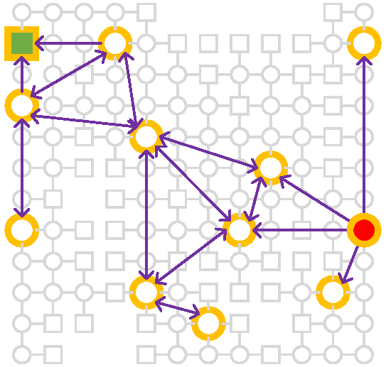
Figure 1: A Proxy Problem on a Grid-World Navigation Task: the MDP of the original problem is in gray and the terminal states are marked with squares. An agent needs to get from the (filled red) position, to the goal (filled green). The agent can reach a distant goal by leveraging a proxy problem with $12$ checkpoints (outlined orange).

A proxy problem can be viewed as a deterministic SMDP, where each directed edge is implemented as a checkpoint-conditioned option. It can be fully described by the discount and reward matrices, $\Gamma^{\pi}$ and $V^{\pi}$, where $\gamma^{\pi}_{ij}$ and $v^{\pi}_{ij}$ are defined as:

$${\color[rgb]{0,0,1}\gamma^{\pi}_{ij}} \doteq\mathbb{E}_{\pi}\left[\gamma^{T_{\perp}}|S_{0}=s_{i},S_{T_{\perp}}=s_{j}\right]$$ (1)

$${\color[rgb]{0,0.5,0}v^{\pi}_{ij}} \doteq\textstyle\mathbb{E}_{\pi}\left[\sum_{t=0}^{T_{\perp}}\gamma^{t}R_{t}|S_{0}=s_{i},S_{T_{\perp}}=s_{j}\right].$$ (2)

By planning with $\Gamma^{\pi}$ and $V^{\pi}$, e.g. using SMDP value iteration (Sutton et al., 1999), we can solve the proxy problem, and form a jumpy plan to travel between states in the original problem. If the proxy problems can be estimated well, the obtained solution will be of good quality, as established in the following theorem:

Theorem 1

Let $\mu$ be the SMDP policy (high-level) and $\pi$ be the low-level policy. Let $\hat{V}^{\pi}$ and $\hat{\Gamma}^{\pi}$ denote learned estimates of the SMDP model. If the estimation accuracy satisfies:

$$|{\color[rgb]{0,0.5,0}v^{\pi}_{ij}}-{\color[rgb]{0,0.5,0}\hat{v}^{\pi}_{ij}}|<\epsilon_{v}v_{\text{max}}\ll(1-\gamma)v_{\text{max}}$$ and (3)

$$\quad\quad|{\color[rgb]{0,0,1}\gamma^{\pi}_{ij}}-{\color[rgb]{0,0,1}\hat{\gamma}^{\pi}_{ij}}|<\epsilon_{\gamma}\ll(1-\gamma)^{2} \forall i,j.$$

Then, the estimated value of the composite $\hat{v}_{\mu\circ\pi}(s)$ is accurate up to error terms linear in $\epsilon_{v}$ and $\epsilon_{\gamma}$:

$$\hat{v}_{\mu\circ\pi}(s) \doteq\sum_{k=0}^{\infty}\hat{v}_{\pi}(s_{k}^{\odot}|{s}_{k+1}^{\odot})\prod_{\ell=0}^{k-1}\hat{\gamma}_{\pi}(s_{\ell}^{\odot}|s_{\ell+1}^{\odot})=v_{\mu\circ\pi}(s)\pm\frac{\epsilon_{v}v_{\text{max}}}{1-\gamma}\pm\frac{\epsilon_{\gamma}v_{\text{max}}}{(1-\gamma)^{2}}+o(\epsilon_{v}+\epsilon_{\gamma})$$

where $\hat{v}_{\pi}(s_{i}|s_{j})\equiv\hat{v}^{\pi}_{ij}$ and $\hat{\gamma}_{\pi}(s_{i}|s_{j})\equiv\hat{\gamma}^{\pi}_{ij}$, and $v_{\text{max}}$ denotes the maximum value.

The theorem indicates that once the agent achieves high accuracy estimation of the model for the proxy problem and a near-optimal lower-level policy ${\color[rgb]{1,0,0}\pi}$, it converges toward optimal performance (proof in Appendix J.2). The theorem also makes no assumption on $\pi$ because it would likely be difficult to learn a good $\pi$ for far away targets. Despite the generality, in the experiments, we limit ourselves to navigation tasks with sparse rewards for reaching goals, where the goals are included as permanent vertices in the proxy problems. This is a case where the accuracy assumption can be met non-trivially, i.e., while avoiding degenerate proxy problems whose edges involve no rewards. Following Thm. 1, we train estimators for $v_{\pi}$ and $\gamma_{\pi}$ and refer to this as edge estimation.

3.2 Design Choices

To plan over proxy problems, our framework embraces the following design choices:

Decision-time planning is employed due to its ability to improve the policy in novel situations;

Spatio-temporal abstraction: temporal abstraction breaks down the given task into smaller ones, while spatial abstraction over the state features improves local learning and generalization;

Higher quality proxies: we introduce pruning techniques to improve the quality of proxy problems;

Learning end-to-end from hindsight, off-policy: to maximize sample efficiency and the ease of training, we propose to use auxiliary (off-)policy methods for edge estimation, and learn a context-conditioned checkpoint generation, both from hindsight experience replay;

Delusion suppression: we propose a delusion suppression technique to minimize the behavior of chasing non-existent outcomes. This is done by exposing the edge estimators to targets that would otherwise not exist in experience.

3.3 Problem 1: Edge Estimation

First, we discuss how to estimate the edges of the proxy problem, given a set of already generated checkpoints. Inspired by conscious information processing in brains (Dehaene et al., 2020) and existing approach in Sylvain et al. (2019), we introduce a local perceptive field selector, $\sigma$, consisting of an attention bottleneck that (soft-)selects the top-$k$ local segments of the full state (e.g. a feature map by a typical convolutional encoder); all segments of the state compete for the $k$ attention slots, i.e. irrelevant aspects of state are discarded, to form a partial state representation (Mott et al., 2019; Tang et al., 2020; Zhao et al., 2021; Alver & Precup, 2023). We provide an example in Fig. 2 (see purple parts). Through $\sigma$, the auxiliary estimators, to be discussed soon, force the bottleneck mechanism to promote aspects relevant to the local estimation of connections between the checkpoints. The rewards and discounts are then estimated from the partial state $\sigma(S)$, based on the agent’s behavior.

3.3.1 Basis for Connections: Checkpoint-Achieving Policy

The low-level policy ${\color[rgb]{1,0,0}\pi}$ maximizes an intrinsic reward, s.t. the target checkpoint $S^{\odot}$ can be reached. The choice of intrinsic reward is flexible; for example, one could use a reward of $+1$ when $S_{t+1}$ is within a small radius of $S^{\odot}$ according to some distance metric, or use reward-respecting intrinsic rewards that enable more sophisticated behaviors, as in (Sutton et al., 2022). In the following, for simplicity, we will denote the checkpoint-achievement condition with equality: $S_{t+1}=S^{\odot}$.

3.3.2 Estimate Connections

We learn the connection estimates with auxiliary reward signals that are designed to be task-invariant (Zhao et al., 2019). These estimates are learned using distributional RL, where the output of each estimator takes the form of a histogram over scalar support (Dabney et al., 2018).

Cumulative Reward. The cumulative discounted task reward $v_{ij}^{\pi}$ is learned by policy evaluation on an auxiliary reward that is the same as the original task reward everywhere except when reaching the target. Given a hindsight sample $\langle x_{t},a_{t},r_{t+1},x_{t+1},x^{\odot}\rangle$ and the corresponding encoded sample $\langle s_{t},a_{t},r_{t+1},s_{t+1},s^{\odot}\rangle$, we train ${\color[rgb]{0,0.5,0}V_{\pi}}$ with KL-divergence as follows:

$${\color[rgb]{0,0.5,0}\hat{v}_{\pi}(\sigma(s_{t}),a_{t}|\sigma(s^{\odot}))}\leftarrow\begin{cases}R(s_{t},a_{t},s_{t+1})+\gamma{\color[rgb]{0,0.5,0}\hat{v}_{\pi}(\sigma(s_{t+1}),a_{t+1}|\sigma(s^{\odot}))}&\text{if }s_{t+1}\neq s^{\odot}\\ R(s_{t},a_{t},s_{t+1})&\text{if }s_{t+1}=s^{\odot}\end{cases}\vspace*{-2mm}$$ (4)

where $\sigma(s)$ is the spatially-abstracted from the full state $s$ and $a_{t+1}\sim{\color[rgb]{1,0,0}\pi(\cdot|\sigma(s_{t+1}),\sigma(s^{\odot}))}$.

Cumulative Distances / Discounts. The cumulative discount leading to the target $s_{\odot}$ under ${\color[rgb]{1,0,0}\pi}$ is unfortunately more difficult to learn than ${\color[rgb]{0,0.5,0}V_{\pi}}$, since the prediction would be heavily skewed towards $1$ if $\gamma\approx 1$. Yet, we can instead effectively estimate cumulative (truncated) distances (or trajectory length) under $\pi$. Such distances can be learned with policy evaluation, where the auxiliary reward is $+1$ on every transition, except at the targets:

$${\color[rgb]{0,0,1}D_{\pi}(\sigma(s_{t}),a_{t}|\sigma(s^{\odot}))}\leftarrow\begin{cases}1+{\color[rgb]{0,0,1}D_{\pi}(\sigma(s_{t+1}),a_{t+1}|\sigma(s^{\odot}))}&\text{if }s_{t+1}\neq s^{\odot}\\ 1&\text{if }s_{t+1}=s^{\odot}\\ \infty&\text{if }s_{t+1}\text{ is terminal and }s_{t+1}\neq s^{\odot}\\ \end{cases}\vspace*{-1mm}$$

where $a_{t+1}\sim{\color[rgb]{1,0,0}\pi(\cdot|\sigma(s_{t+1}),\sigma(s^{\odot}))}$. The cumulative discount is then recovered by replacing the support of the output distance histogram with the corresponding discounts. Additionally, the learned distance is used to prune unwanted checkpoints to simplify the proxy problem, as well as prune far-fetched edges. The details of pruning will be presented shortly.

Please refer to the Appendix J.1 for the properties of the learning rules for $\hat{v}_{\pi}$ and $\hat{\gamma}_{\pi}$.

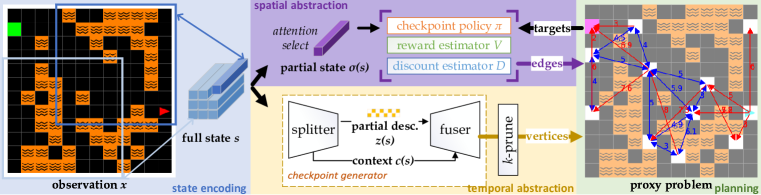
Figure 2: Skipper Framework: 1) Partial states consist of a few local fields, soft-selected via top-$k$ attention (Gupta et al., 2021). Skipper’s edge estimations and low-level behaviors $\pi$ are based on the partial states. 2) The checkpoint generator learns by splitting the full state into context and partial descriptions, and fusing them to reconstruct the input. It generates checkpoints by sampling partial descriptions and combines them with the episodic contexts; 3) We prune the vertices and edges of the denser graphs to extract sparser proxy problems. Once a plan is formed, the immediate checkpoint target is used to condition the policy. In the proxy problem example, blue edges are estimated to be bidirectional and red edges have the other direction pruned.

3.4 Problem 2: Vertex Generation

The checkpoint generator aims to directly model the possible future states without needing to know how exactly the agent might reach them. The details of checkpoint transitions will be abstracted by the connection estimates instead.

To make the checkpoint generator generalize well across diverse tasks, while still being able to capture the underlying causal mechanisms in the environment (a challenge for existing model-based methods) (Zhang et al., 2020), we propose that the checkpoint generator learns to split the state representation into two parts: an episodic context and a partial description. In a navigation problem, for example, as in Fig. 2, a context could be a representation of the map of a gridworld, and the partial description be the 2D-coordinates of the agent’s location. In different contexts, the same partial description could correspond to very different states. Yet, within the same context, we should be able to recover the same state given the same partial description.

As shown in Fig. 2, this information split is achieved using two functions: the splitter $\mathcal{E}_{CZ}$, which maps the input state $S$ into a representation of a context $c(S)$ and a partial description $z(S)$, as well as the fuser $\bigoplus$ which, when applied to the input $\langle c,z\rangle$, recovers $S$. In order to achieve consistent context extraction across states in the same episode, at training time, we force the context to be extracted from other states in the same episode, instead of the input.

We sample in hindsight a diverse distribution of target encoded (full) states $S^{\odot}$, given any current $S_{t}$. Hence, we use as generator a conditional Variational AutoEncoder (VAE) (Sohn et al., 2015) which learns a distribution $p(S^{\odot}|C(S_{t}))=\sum_{z}{p(S^{\odot}|C(S_{t}),z)p(z|C(S_{t}))}$, where $C(S_{t})$ is the extracted context from $S_{t}$ and $z$s are the partial descriptions. We train the generator by minimizing the evidence lower bound on $\langle S_{t},S^{\odot}\rangle$ pairs chosen with HER.

Similarly to Hafner et al. (2023), we constrain the partial description as a bundle of binary variables and train them with the straight-through gradients (Bengio et al., 2013). These binary latents can be easily sampled or composed for generation. Compared to models such as that in Director (Hafner et al., 2022), which generates intermediate goals given the on-policy trajectory, ours is expected to generate a more diverse distribution of states, beneficial for planning in novel scenarios.

3.4.1 Pruning

In this paper,we limit ourselves only to checkpoints from a return-unaware conditional generation model, leaving the question of how to improve the quality of the generated checkpoints for future work. Without learning, the proxy problem can be improved by making it more sparse, and making the proxy problem vertices more evenly spread in state space. To achieve this, we propose a pruning algorithm based on $k$-medoids clustering (Kaufman & Rousseeuw, 1990), which requires pairwise distance estimates between states. During proxy problem construction, we first sample a larger number of checkpoints, and then cluster them and select the centers (which are always real states).

Notably, for sparse reward tasks, the generator cannot guarantee the presence of the rewarding checkpoints in the proposed proxy problem. We could remedy this by explicitly learning the generation of the rewarding states with another conditional generator. These rewarding states should be kept as vertices (immune from pruning).

In addition to pruning the vertices, we also prune the edges according to a distance threshold, i.e., all edges with estimated distance over the threshold are deleted from the complete graph of the pruned vertices. This biases potential plans towards shorter-length, smaller-scale sub-problems, as far-away checkpoints are difficult for $\pi$ to achieve.

3.4.2 Safety & Delusion Control

Model-based HRL agents can be prone to blindly optimizing for objectives without understanding the consequences (Langosco et al., 2022; Paolo et al., 2022). We propose a technique to suppress delusions by exposing the edge estimators to potentially delusional targets that do not exist in the experience replay buffer. Details and examples are provided in the Appendix.

3.5 Overall Framework & Training

An intuitive overall algorithm and the training details are presented in Appendix H. The estimators are trained with KL-divergence and equal weighting of all terms, and the generator is trained with a VAE loss ,where the overall training loss is a simple sum of the aforementioned.

4 Related Works & Discussions

Temporal Abstraction. Resembling attention in human consciousness, choosing a checkpoint target is a selection towards certain decision points in the dimension of time, i.e. a form of temporal abstraction. Constraining options, Skipper learns the options targeting certain “outcomes”, which dodges the difficulties of option collapse (Bacon et al., 2017) and option outcome modelling by design. The constraints indeed shift the difficulties to generator learning (Silver & Ciosek, 2012; Tang & Salakhutdinov, 2019). We expect this to entail benefits where states are easy to learn and generate, and / or in stochastic environments where the outcomes of unconstrained options are difficult to learn. Constraining options was also investigated in Sharma et al. (2019) in an unsupervised setting.

Spatial Abstraction is different from “state abstraction” (Sacerdoti, 1974; Knoblock, 1994), which evolved to be a more general concept that embraces mainly the aspect of state aggregation, i.e. state space partitioning (Li et al., 2006). Spatial abstraction, defined to capture the behavior of attention in conscious planning in the spatial dimensions, focuses on the within-state partial selection of the environmental state for decision-making. It corresponds naturally to the intuition that state representations should contain useful aspects of the environment, while not all aspects are useful for a particular intent. Efforts toward spatial abstraction are traceable to early hand-coded proof-of-concepts proposed in e.g. Dietterich (2000). Until only recently, attention mechanisms had primarily been used to construct state representations in model-free agents for sample efficiency purposes, without the focus on generalization (Mott et al., 2019; Manchin et al., 2019; Tang et al., 2020). In Fu et al. (2021); Zadaianchuk et al. (2020); Shah et al. (2021), $3$ more recent model-based approaches, spatial abstractions are attempted to remove visual distractors. Concurrently, emphasizing on generalization, our previous work (Zhao et al., 2021) used spatially-abstract partial states in decision-time planning. We proposed an attention bottleneck to dynamically select a subset of environmental entities during the atomic-step forward simulation, without explicit goals provided as in Zadaianchuk et al. (2020). Skipper’s checkpoint transition is a step-up from our old approach, where we now show that spatial abstraction, an overlooked missing flavor, is as crucial for longer-term planning as temporal abstraction (Konidaris & Barto, 2009).

Task Abstraction via Goal Composition The early work McGovern & Barto (2001) suggested to use bottleneck states as subgoals to abstract given tasks into manageable steps. Nair et al. (2018); Florensa et al. (2018) use generative model to imagine subgoals while Eysenbach et al. (2019) search directly on the experience replay. In Kim et al. (2021), promising states to explore are generated and selected with shortest-path algorithms. Similar ideas have been attempted for guided exploration (Erraqabi et al., 2021; Kulkarni et al., 2016). Similar to Hafner et al. (2022), Czechowski et al. (2021) generate fixed-steps ahead subgoals for reasoning tasks, while Bagaria et al. (2021) augments the search graph by states reached fixed-steps ahead. Nasiriany et al. (2019); Xie et al. (2020); Shi et al. (2022) employ CEM to plan a chain of subgoals towards the task goal (Rubinstein, 1997b). Skipper utilizes proxy problems to abstract the given tasks via spatio-temporal abstractions (Bagaria et al., 2021). Checkpoints can be seen as sub-goals that generalize the notion of “landmarks” or “waypoints” in Sutton et al. (1999); Dietterich (2000); Savinov et al. (2018). Zhang et al. (2021) used latent landmark graphs as high-level guidance, where the landmarks are sparsified with weighted sums in the latent space to compose subgoals. In comparison, our checkpoint pruning selects a subset of generated states, which is less prone to issues created by weighted sums.

Planning Estimates. Zhang et al. (2021) propose a distance estimate with an explicit regression. With TDMs (Pong et al., 2018), LEAP (Nasiriany et al., 2019) embraces a sparse intrinsic reward based on distances to the goal. Contrasting with our distance estimates, there is no empirical evidence of TDMs’ compatibility with stochasticity and terminal states. Notably, Eysenbach et al. (2019) employs a similar distance learning scheme to learn the shortest path distance between states found in the experience replay; while our estimators learn the distance conditioned on evolving policies. Such aspect was also investigated in Nachum et al. (2018).

Decision-Time HP Methods. Besides LEAP (Nasiriany et al., 2019), decision-time planning with evolutionary algorithms was investigated in Nair & Finn (2020); Hafner et al. (2019).

5 Experiments

As introduced in Sec. 2, our first goal is to test the zero-shot generalization ability of trained agents. To fully understand the results, it is necessary to have precise control of the difficulty of the training and evaluation tasks. Also, to validate if the empirical performance of our agents matches the formal analyses (Thm. 1), we need to know how close to the (optimal) ground truth our edge estimations and checkpoint policies are. These goals lead to the need for environments whose ground truth information (optimal policies, true distances between checkpoints, etc) can be computed. Thus, we base our experimental setting on the MiniGrid-BabyAI framework Chevalier-Boisvert et al. (2018b; a); Hui et al. (2020). Specifically, we build on the experiments used in our previous works Zhao et al. (2021); Alver & Precup (2022): the agent needs to navigate to the goal from its initial state in gridworlds filled with terminal lava traps generated randomly according to a difficulty parameter, which controls their density. During evaluation, the agent is always spawned at the opposite side from the goals. During training, the agent’s position is uniformly initialized to speed up training. We provide results for non-uniform training initialization in the Appendix.

These fully observable tasks prioritize on the challenge of reasoning over causal mechanisms over learning representations from complicated observations, which is not the focus of this work. Across all experiments, we sample training tasks from an environment distribution of difficulty $0.4$: each cell in the field has probability $0.4$ to be filled with lava while guaranteeing a path from the initial position to the goal. The evaluation tasks are sampled from increasing OOD difficulties of $0.25$, $0.35$, $0.45$ and $0.55$, where the training difficulty acts as a median. To step up the long(er) term generalization difficulty compared to existing work, we conduct experiments done on large, $12\times 12$ maze sizes, (see the visualization in Fig 2). The agents are trained for $1.5\times 10^{6}$ interactions.

We compare Skipper against two state-of-the-art Hierarchical Planning (HP) methods: LEAP (Nasiriany et al., 2019) and Director (Hafner et al., 2022). The comparative results include:

• Skipper-once: A Skipper agent that generates one proxy problem at the start of the episode, and the replanning (choosing a checkpoint target based on the existing proxy problem) only triggers a quick selection of the immediate checkpoint target;

• Skipper-regen: A Skipper agent that regenerates a proxy problem when replanning is triggered;

• modelfree: A model-free baseline agent sharing the same base architecture with the Skipper variants, with a prioritized distributional Double DQN (Dabney et al., 2018; Van Hasselt et al., 2016);

• Director: A tuned Director agent (Hafner et al., 2022) fed with simplified visual inputs. Since Director discards trajectories that are not long enough for training purposes, we make sure that the same amount of training data is gathered as for the other agents;

• LEAP: A re-implemented LEAP for discrete action spaces. Due to low performance, we replaced the VAE and the distance learning mechanisms with our counterparts. We waived the interaction costs for its generator pretraining stage, only showing the second stage of RL pretraining.

Please refer to the Appendix for more details and insights on these agents.

5.1 Generalization Performance

Fig. 3 shows how the agents’ generalization performance evolves during training. These results are obtained with $50$ fixed sampled training tasks (different for each seed), a representative configuration of different numbers of training tasks including $\{1,5,25,50,100,\infty\}$, whose results are in the Appendix. In Fig. 3 a), we observe how well an agent performs on its training tasks. If an agent performs well here but badly in b), c), d) and e), e.g. the modelfree baseline, then we suspect that it overfitted on training tasks, likely an indicator of reliance on memorization (Cobbe et al., 2020).

We observe a (statistically-)significant advantage in the generalization performance of the Skipper agents throughout training. We have also included significance tests and power analyses (Colas et al., 2018; Patterson et al., 2023) in the Appendix, together with results for other training configurations. The regen variant exhibits dominating performance over all others. This is because the frequent reconstruction of the graph makes the agent less prone to being trapped in a low-quality proxy problem and provides extra adaptability in novel scenarios (more discussions in the Appendix). Skippers behave less optimally than expected during training, despite the strong generalization on evaluation tasks. As our ablation results and theoretical analyses consistently show, such a phenomenon is a composite outcome of inaccuracies both in the proxy problem and the checkpoint policy. One major symptom of an inaccurate proxy problem is that the agent would chase delusional targets. We address this behavior with a delusion suppression technique, to be discussed in the Appendix.

(a) training, diff $0.4$

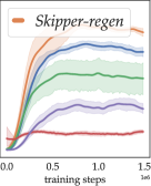
(b) OOD, diff $0.25$

(c) OOD, diff $0.35$

(d) OOD, diff $0.45$

(e) OOD, diff $0.55$

Figure 3: Generalization Performance of Agents During Training: the $x$-axes correspond to training progress, while the aligned $y$-axes represent the success rate of episodes (optimal is 1.0). Each agent is trained with $50$ tasks. Each data point is the average success rate over $20$ evaluation episodes, and each error bar (95% confidence interval) is processed from $20$ independent seed runs. Training tasks performance is shown in (a) while OOD performance is shown in (b), (c), (d), (e).

Better than the modelfree baseline, LEAP obtains reasonable generalization performance, despite the extra budget it needs for pretraining. In the Appendix, we show that LEAP benefits largely from the delusion suppression technique. This indicates that optimizing for a path in the latent space is prone to errors caused by delusional subgoals. Lastly, we see that the Director agents suffer in these experiments despite their good performance in the single environment experimental settings reported by Hafner et al. (2022). We present additional experiments in the Appendix to show that Director is ill-suited for our generalization-focused setting: Director still performs well in single environment configurations, but its performance deteriorates fast with more training tasks. This indicates poor scalability in terms of generalization, a limitation to its application in real-world scenarios.

5.2 Scalability of Generalization Performance

Like Cobbe et al. (2020), we investigate the scalability of the agents’ generalization abilities across different numbers of training tasks. To this end, in Fig. 4, we present the results of the agents’ final evaluation performance after training over different numbers of training tasks.

With more training tasks, Skippers and the baseline show consistent improvements in generalization performance. While both LEAP and Director behave similarly as in the previous subsection, notably, the modelfree baseline can reach similar performance as Skipper, but only when trained on a different task in each episode, which is generally infeasible in the real world beyond simulation.

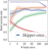
(a) training, diff $0.4$

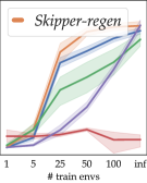
(b) OOD, diff $0.25$

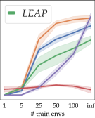
(c) OOD, diff $0.35$

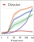
(d) OOD, diff $0.45$

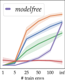
(e) OOD, diff $0.55$

Figure 4: Generalization Performance of Agents on Different Numbers of Training Tasks: each data point and corresponding error bar (95% confidence interval) are based on the final performance from $20$ independent seed runs. Training task performance is shown in (a) while OOD performance is shown in (b), (c), (d), (e). Notably, the Skipper agents as well as the adapted LEAP behave poorly during training when being trained on only one task, as the split of context and partial information cannot be achieved. Training on one task invalidates the purpose of the proposed generalization-focused checkpoint generator.

5.3 Ablation & Sensitivity Studies

In the Appendix, we present ablation results confirming the effectiveness of delusion suppression, $k$-medoids pruning and the effectiveness of spatial abstraction via the local perception field. We also provide sensitivity study for the number of checkpoints in each proxy problem.

5.4 Summary of Experiments

Within the scope of the experiments, we conclude that the proposed framework provides benefits for generalization; And it achieves better generalization when exposed to more training tasks;

From the content presented in the Appendix, we deduce additionally that:

• Spatial abstraction based on the local perception field is crucial for the scalability of the agents;

• Skipper performs well by reliably decomposing the given tasks, and achieving the sub-tasks robustly. Its performance is bottlenecked by the accuracy of the estimated proxy problems as well as the checkpoint policies, which correspond to goal generalization and capability generalization, respectively, identified in Langosco et al. (2022). This matches well with our theory. The proposed delusion suppression technique (in Appendix) is effective in suppressing plans with non-existent checkpoints as targets, thereby increasing the accuracy of the proxy problems;

• LEAP fails to generalize well within its original form and can generalize better when combined with the ideas proposed in this paper; Director may generalize better only in domains where long and informative trajectory collection is possible;

• We verified empirically that, as expected, Skipper is compatible with stochasticity.

6 Conclusion & Future Work

Building on previous work on spatial abstraction (Zhao et al., 2021), we proposed, analyzed and validated Skipper, which generalizes its learned skills better than the compared methods, due to its combinned spatio-temporal abstractions. A major unsatisfactory aspect of this work is that we generated checkpoints at random by sampling the partial description space. Despite the pruning mechanisms, the generated checkpoints, and thus temporal abstraction, do not prioritize the predictable, important states that matter to form a meaningful plan (Şimşek & Barto, 2004). We would like to continue investigating the possibilities along this line. Additionally, we would like to explore other environments where the accuracy assumption (in Thm. 1) can meaningfully hold, i.e. beyond sparse reward cases.

Appendix A Experimental Results (Cont.)

We present the experimental results that the main paper could not hold due to the page limit.

A.1 Skipper-once Scalability

We present the performance of Skipper-once on different numbers of training tasks in Fig. 5.

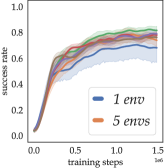
(a) training, diff $0.4$

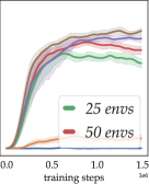
(b) OOD, diff $0.25$

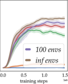
(c) OOD, diff $0.35$

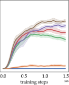
(d) OOD, diff $0.45$

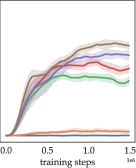
(e) OOD, diff $0.55$

Figure 5: Generalization Performance of Skipper-once on different numbers of training tasks: each error bar (95% confidence interval) is obtained from $20$ independent seed runs.

A.2 Skipper-regen Scalability

We present the performance of Skipper-regen on different numbers of training tasks in Fig. 6.

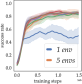
(a) training, diff $0.4$

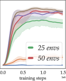
(b) OOD, diff $0.25$

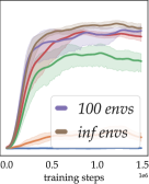
(c) OOD, diff $0.35$

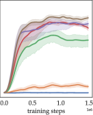
(d) OOD, diff $0.45$

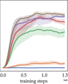
(e) OOD, diff $0.55$

Figure 6: Performance of Skipper-regen on different numbers of training tasks: each error bar (95% confidence interval) is obtained from $20$ independent seed runs.

A.3 modelfree Baseline Scalability

We present the performance of the modelfree baseline on different numbers of training tasks in Fig. 7.

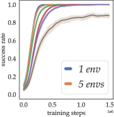
(a) training, diff $0.4$

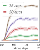
(b) OOD, diff $0.25$

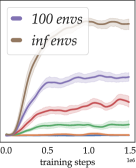
(c) OOD, diff $0.35$

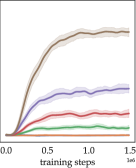
(d) OOD, diff $0.45$

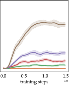
(e) OOD, diff $0.55$

Figure 7: Generalization Performance of the modelfree baseline on different numbers of training tasks: each error bar (95% confidence interval) is obtained from $20$ independent seed runs.

A.4 LEAP Scalability

We present the performance of the adapted LEAP baseline on different numbers of training tasks in Fig. 8.

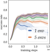
(a) training, diff $0.4$

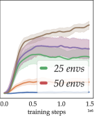
(b) OOD, diff $0.25$

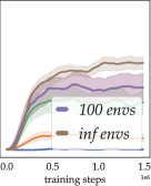
(c) OOD, diff $0.35$

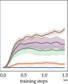
(d) OOD, diff $0.45$

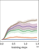
(e) OOD, diff $0.55$

Figure 8: Generalization Performance of the LEAP baseline on different numbers of training tasks: each error bar (95% confidence interval) is obtained from $20$ independent seed runs.

A.5 Director Scalability

We present the performance of the adapted Director baseline on different numbers of training tasks in Fig. 9.

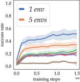
(a) training, diff $0.4$

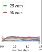
(b) OOD, diff $0.25$

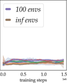
(c) OOD, diff $0.35$

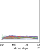
(d) OOD, diff $0.45$

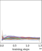
(e) OOD, diff $0.55$

Figure 9: Generalization Performance of the Director baseline on different numbers of training tasks: each error bar (95% confidence interval) is obtained from $20$ independent seed runs.

A.6 Comparative Generalization Performance on Different Numbers of Training Tasks

The comparative results of all agents performing on each training configurations, i.e. different numbers of training tasks, are presented in Fig. 10, Fig. 11, Fig. 12, Fig. 13, Fig. 14 and Fig. 15.

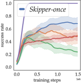
(a) training, diff $0.4$

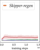
(b) OOD, diff $0.25$

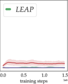
(c) OOD, diff $0.35$

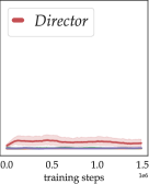
(d) OOD, diff $0.45$

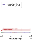
(e) OOD, diff $0.55$

Figure 10: Generalization Performance of the Agents when trained with $1$ training task: each error bar (95% confidence interval) is obtained from $20$ independent seed runs.

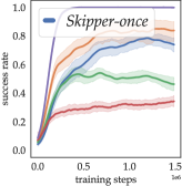
(a) training, diff $0.4$

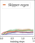
(b) OOD, diff $0.25$

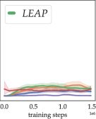
(c) OOD, diff $0.35$

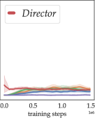
(d) OOD, diff $0.45$

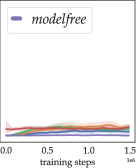
(e) OOD, diff $0.55$

Figure 11: Generalization Performance of the Agents when trained with $5$ training tasks: each error bar (95% confidence interval) is obtained from $20$ independent seed runs.

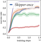
(a) training, diff $0.4$

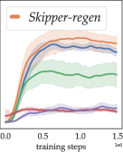
(b) OOD, diff $0.25$

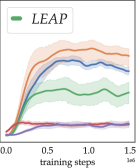
(c) OOD, diff $0.35$

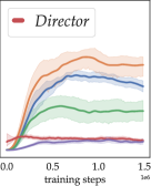
(d) OOD, diff $0.45$

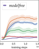
(e) OOD, diff $0.55$

Figure 12: Generalization Performance of the Agents when trained with $25$ training tasks: each error bar (95% confidence interval) is obtained from $20$ independent seed runs.

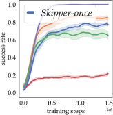
(a) training, diff $0.4$

(b) OOD, diff $0.25$

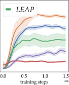
(c) OOD, diff $0.35$

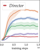
(d) OOD, diff $0.45$

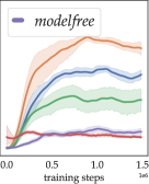
(e) OOD, diff $0.55$

Figure 13: Generalization Performance of the Agents when trained with $50$ training tasks (same as in the main paper): each error bar (95% confidence interval) is obtained from $20$ independent seed runs.

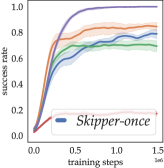
(a) training, diff $0.4$

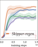
(b) OOD, diff $0.25$

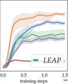
(c) OOD, diff $0.35$

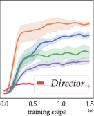
(d) OOD, diff $0.45$

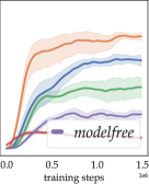
(e) OOD, diff $0.55$

Figure 14: Generalization Performance of the Agents when trained with $100$ training tasks: each error bar (95% confidence interval) is obtained from $20$ independent seed runs.

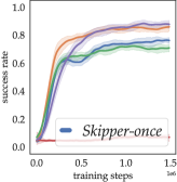
(a) training, diff $0.4$

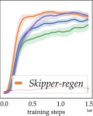
(b) OOD, diff $0.25$

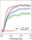
(c) OOD, diff $0.35$

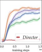
(d) OOD, diff $0.45$

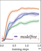
(e) OOD, diff $0.55$

Figure 15: Generalization Performance of the Agents when trained with $\infty$ training tasks (a new task each training episode): each error bar (95% confidence interval) is obtained from $20$ independent seed runs.

A.6.1 Statistical Significance & Power Analyses

Besides visually observing generally non-overlapping confidence intervals, we present the pairwise $t$-test results of Skipper-once and Skipper-regen against the other methods, as well as, if significant, power analyses to determine if the number of seed runs ($20$) was enough to make the significance claim. These results are shown in Tab. 1 and Tab. 2, respectively.

Table 1: Skipper-once v.s. others: significance & power

	method / difficulty	0.25	0.35	0.45	0.55
1 train envs	leap	22	NO	NO	NO
	director	15	11	22	11
	baseline	NO	38	36	NO
5 train envs	leap	28	NO	NO	NO
	director	NO	NO	NO	22
	baseline	11	8	10	12
25 train envs	leap	15	13	11	7
	director	2	2	2	2
	baseline	2	2	2	2
50 train envs	leap	17	16	11	11
	director	2	2	2	2
	baseline	2	2	2	2
100 train envs	leap	15	10	7	9
	director	2	2	2	2
	baseline	2	2	2	2
inf train envs	leap	32	5	7	3
	director	2	2	2	2
	baseline	NO	NO	NO	NO
$t$-test significance is set to be $0.05$.
Effect size equals to the difference of the means of the compared pairs (Colas et al., 2018).
For significant comparisons, the minimum number of seeds to achieve statistical power $0.2$ is provided.
Cells are marked bold if results not significant or not enough seeds to achieve statistical power.

As we can observe from the tables, generally there is significant evidence of generalization advantage in Skipper variants compared to the other methods, especially when the number of training environments are between $25$ to $100$. Additionally, as expected, Skipper-regen displays more dominating performance compared to that of Skipper-once.

Table 2: Skipper-regen v.s. others: significance & power

	method / difficulty	0.25	0.35	0.45	0.55
1 train envs	leap	32	NO	NO	NO
	director	16	13	23	10
	baseline	NO	NO	NO	NO
5 train envs	leap	NO	NO	NO	NO
	director	33	NO	NO	NO
	baseline	6	8	4	5
25 train envs	leap	10	7	5	4
	director	2	2	2	2
	baseline	2	2	2	2
50 train envs	leap	6	4	3	3
	director	2	2	2	2
	baseline	2	2	2	2
100 train envs	leap	7	3	3	2
	director	2	2	2	2
	baseline	2	2	2	2
inf train envs	leap	15	3	2	2
	director	2	2	2	2
	baseline	NO	NO	35	5
$t$-test significance is set to be $0.05$.
Effect size equals to the difference of the means of the compared pairs (Colas et al., 2018).
For significant comparisons, the minimum number of seeds to achieve statistical power $0.2$ is provided.
Cells are marked bold if results not significant or not enough seeds to achieve statistical power.

Appendix B Ablation & Sensitivity

B.1 Validation of Effectiveness on Stochastic Environments

We present the performance of the agents in stochastic variants of the used environment. Specifically, in these tasks, with probability $0.1$ where each action an agent takes could be changed into a random action. We present the $50$-training tasks performance evolution in Fig. 16. The results validate the compatibility of our agents with stochasticity in environmental dynamics. Notably, the performance of the baseline deteriorated to worse than even Director with the injected stochasticity. The compatibility of Hierarchical RL frameworks to stochasticity has been investigated in Hogg et al. (2009).

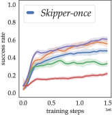
(a) training, diff $0.4$

(b) OOD, diff $0.25$

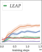
(c) OOD, diff $0.35$

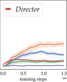
(d) OOD, diff $0.45$

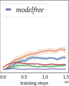
(e) OOD, diff $0.55$

Figure 16: Generalization Performance of agents in stochastic environments: $\epsilon$-greedy style randomness is added to each primitive action with $\epsilon=0.1$. Each agent is trained with $50$ environments and each curve is processed from $20$ independent seed runs.

B.2 Ablation for Spatial Abstraction

We present in Fig. 17 the ablation results on the spatial abstraction component with Skipper-once agent, trained with $50$ tasks. The alternative component of the attention-based bottleneck, which is without the spatial abstraction, is an MLP on a flattened full state. The results confirm significant advantage in terms of generalization performance as well as learning speed, brought by the introduced spatial abstraction technique.

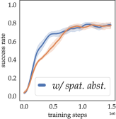
(a) training, diff $0.4$

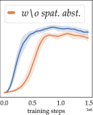
(b) OOD, diff $0.25$

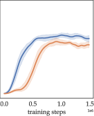
(c) OOD, diff $0.35$

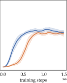
(d) OOD, diff $0.45$

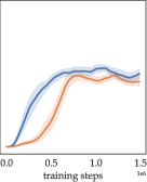
(e) OOD, diff $0.55$

Figure 17: Ablation for Spatial Abstraction on Skipper-once agent: each agent is trained with $50$ environments and each curve is processed from $20$ independent seed runs.

B.3 Accuracy of Proxy Problems & Checkpoint Policies

We present in Fig. 18 the ablation test results on the accuracy of proxy problems as well as the checkpoint policies of the Skipper-once agents, trained with $50$ tasks. The ground truths are computed via Dynamic Programming (DP) on the optimal policies, which are also suggested by DP. Concurring with our theoretical analyses, the results indicate that the performance of Skipper is determined (bottlenecked) by the accuracy of the proxy problem estimation on the high-level and the optimality of the checkpoint policy on the lower level. Specifically, the curves for the generalization performance across training tasks, as in (a) of 18, indicate that the lower than expected performance is a composite outcome of errors in the two levels. In the next part, we address a major misbehavior of inaccurate proxy problem estimation - chasing delusional targets.

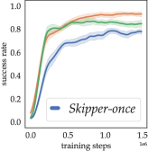
(a) training, diff $0.4$

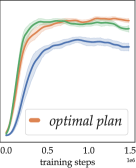
(b) OOD, diff $0.25$

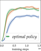
(c) OOD, diff $0.35$

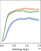
(d) OOD, diff $0.45$

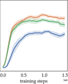
(e) OOD, diff $0.55$

Figure 18: Skipper-once Empirical Performance v.s. ground truths: both the optimal policy and optimal plan variants are calculated via DP on the environment dynamics. The default deterministic setting induces the fact that combining optimal policy and optimal plan results in $1.0$ success rate. The figures suggest that the learned agent is limited by errors both in the proxy problem estimation and the checkpoint policy $\pi$. Each agent is trained with $50$ environments and each curve is processed from $20$ independent seed runs.

B.4 Training Initialization: uniform v.s. same as evaluation

We present in Fig. 19 the comparative results on the training setting: whether to use uniform initial state distribution or not. The non-uniform starting state distributions introduce additional difficulties in terms of exploration and therefore globally slow down the learning process. These results are obtained from training on $50$ tasks. We conclude that given similar computational budget, using non-uniform initialization only slows down the learning curves, and thus we use the ones with uniform initialization for presentation in the main paper.

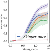
(a) training, diff $0.4$

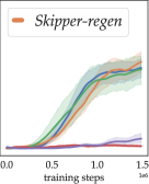
(b) OOD, diff $0.25$

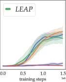
(c) OOD, diff $0.35$

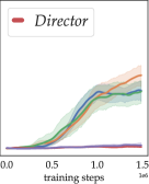
(d) OOD, diff $0.45$

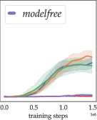
(e) OOD, diff $0.55$

Figure 19: Comparative Results on $50$ training tasks without uniform initial state distribution: each curve is processed from $20$ independent seed runs.

B.5 Ablation: Vertex Pruning

As mentioned previously, each proxy problem in the experiments are reduced from $32$ vertices to $12$ with such techniques. We present the comparative performance curves of the used configuration against a baseline that generates $12$-vertex proxy problems without pruning. We present in Fig. 20 these ablation results on the component of $k$-medoids checkpoint pruning. We observe that the pruning not only increases the generalization but also the stability of performance.

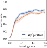
(a) training, diff $0.4$

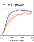
(b) OOD, diff $0.25$

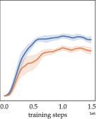
(c) OOD, diff $0.35$

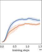
(d) OOD, diff $0.45$

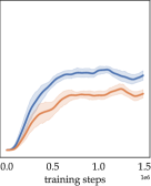
(e) OOD, diff $0.55$

Figure 20: Ablation Results on $50$ training tasks for $k$-medoids pruning: each curve is processed from $20$ independent seed runs.

B.6 Sensitivity: Number of Vertices

We provide a sensitivity analysis to the number of checkpoints (number of vertices) in each proxy problem. We present the results of Skipper-once on $50$ training tasks with different numbers of post-pruning checkpoints (all reduced from $32$ by pruning), in Fig. 21. From the results, we can see that as long as the number of checkpoints is above $6$, Skipper exhibits good performance. We therefore chose $12$, the one with minimal computation cost, as the default hyperparameter.

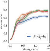
(a) training, diff $0.4$

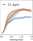
(b) OOD, diff $0.25$

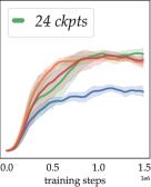
(c) OOD, diff $0.35$

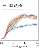
(d) OOD, diff $0.45$

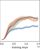
(e) OOD, diff $0.55$

Figure 21: Sensitivity of Skipper-once on the number of checkpoints in each proxy problem: each agent is trained with $50$ environments. All curves are processed from $20$ independent seed runs.

B.7 Ablation: Planning over Proxy Problems

We provide additional results to intuitively understand the effectiveness of planning over proxy problems. This is done by comparing the results of Skipper-once with a baseline Skipper-goal that blindly selects the task goal as its target all the time. We present the results based on $50$ training tasks in Fig. 22. Concurring with our vision on temporal abstraction, we can see that solving more manageable sub-problems leads to faster convergence. The Skipper-goal variant catches up later when the policy slowly improves to be capable of solving long distance navigation.

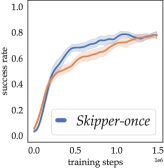
(a) training, diff $0.4$

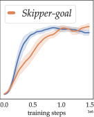
(b) OOD, diff $0.25$

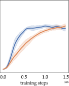
(c) OOD, diff $0.35$

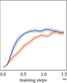
(d) OOD, diff $0.45$

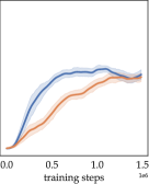
(e) OOD, diff $0.55$

Figure 22: Effectiveness of Proxy Problem based Planning: each agent is trained with $50$ environments and each curve is processed from $20$ independent seed runs.

// This whole code block should be injected into the training loop if used

generate using the checkpoint generator, from the sampled batch of encoded states, the target states (to overwrite those relabelled in the HER) i.e. replace $\langle s_{t},a_{t},r_{t+1},s_{t+1},s^{\odot}\rangle$ with $\langle s_{t},a_{t},r_{t+1},s_{t+1},s^{\odot}_{*}\rangle$, where $s^{\odot}_{*}$ are generated from the context of $s_{t}$

train the distance estimator $D$ as if these are sampled from the HER

Algorithm 1 Delusion Suppression

Appendix C Delusion Suppression

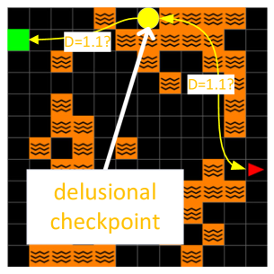
Figure 23: Example of Failure Caused by Delusions: we illustrate an instance of chasing delusional checkpoint in one of our experimental runs by Skipper. The distance (discount) estimator, probably due to the ill-generalization, estimates that the delusional checkpoint (yellow) is very close to every other state. A resulting plan was that the agent thought it could reach any far-away checkpoints by using the delusional state to form a shortcut: the goal that was at least $17$ steps away would be reached in $2.2$.

RL agents are prone to blindly optimizing for an intrinsic objective without fully understanding the consequences of its actions. Particularly in model-based RL or in Hierarchical RL (HRL), there is a significant risk posed by the agents trying to achieve delusional future states that do not exist within the safety constraints. With a use of a learned generative model, as in the proposed framework, such risk is almost inevitable, because of uncontrollable generalization effects.

Generalization abilities of the generative models are a double-edged sword. The agent would take advantage of its potentials to propose novel checkpoints to improve its behavior, but is also at risk of wanting to achieve non-existent unknown consequences. In our framework, checkpoints proposed by the generative model could correspond to non-existent “states” that would lead to delusional edge estimates and therefore confuse planning. For instance, arbitrarily sampling partial descriptions may result in a delusional state where the agent is in a cell that can never be reached from the initial states. Since such states do not exist in the experience replay, the estimators will have not learned how to handle them appropriately when encountered in the generated proxy problem during decision time. We present a resulting failure mode in Fig. 23.

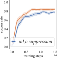
(a) generalization performance across training tasks

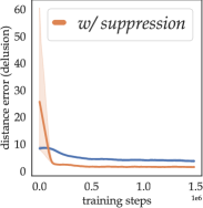
(b) distance estimation error (L1) for delusional edges

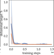
(c) frequency of selecting delusional targets

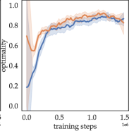
(d) target optimality

Figure 24: Ablation Results for Skipper-once with the proposed Delusion Suppression Technique: each curve and corresponding error bar (95% CI) are processed from $20$ independent seed runs. a) the performance across training tasks is shown. A more optimal performance can be achieved with Skipper-once in training tasks, when delusions are suppressed; b) During training interactions, the error in estimated (truncated) distance from and to delusional targets are significantly reduced with the technique; c) The frequency of selecting a delusional target is reduced to almost negligible during the whole training process; d) The optimality of target checkpoint during training can be improved by the suppression. Each agent is trained with $50$ environments and each curve is processed from $20$ independent seed runs.

To address such concerns, we propose an optional auxiliary training procedure that makes the agent stay further away from delusional checkpoints. Due to the favorable properties of the update rules of $D_{\pi}$ (in fact, $V_{\pi}$ as well), all we have to do is to replace the hindsight-sampled target states with generated checkpoints, which contain non-existent states. Then, the auxiliary rewards will all converge to the minimum in terms of favorability on the non-existent states. This is implemented trivially by adding a loss to the original training loss for the distance estimator, which we give a $0.25$ scaling for stability.

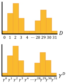
Figure 25: Estimating Distributions of Discount and Distance with the Same Histogram: by transplanting the support with the corresponding discount values, the distribution of the cumulative discount can be inferred.

We provide analytic results and related discussion for Skipper-once agents trained with the proposed delusion suppression technique on $50$ training tasks in Fig. 24. The delusion suppression technique is not enabled by default because it was not introduced in the main manuscript due to the page limits.

The delusion suppression technique can also be used to help us understand the failure modes of LEAP, which can be found in the later contents.

Appendix D Recovering Discounts

We can recover the distribution of the cumulative discount by replacing the support of the discretized truncated distances with the corresponding discounts, as shown in Fig. 25. Specifically, the problem we wanted to dodge was $\mathbb{E}[\gamma^{D}]\neq\gamma^{\mathbb{E}[D]}$. Luckily, the probability of having a trajectory length of 4 under policy $\pi$ from state $s_{t}$ to $s_{\odot}$ is the same as a trajectory having discount $\gamma^{4}$. The estimated distribution over distances is used to recover on a different support the corresponding distribution of discounts.

Appendix E Skipper Implementation Details

The PyTorch-based source code of experiments is uploaded in the supplementary materials, where reviewers could find the detailed architectures that may be difficult to understand from the following descriptions. The hyperparameters introduced by Skipper can be located in Alg. 2.

The agent is based on a distributional prioritized double DQN. All the trainable parameters are optimized with Adam at a rate of $2.5\times 10^{-4}$ (Kingma & Ba, 2014), with a gradient clipping by value (maximum absolute value $1.0$). The priorities for experience replay sampling are equal to the per-sample training loss, which is a sum of all KL-divergences of the estimators (cross-entropy for the termination estimator), and the ELBO loss of the checkpoint generator.

E.1 Full State Encoder

The full-state encoder is a two layered residual block (with kernel size 3 and doubled intermediate channels) combined with the $16$-dimensional bag-of-words embedder of BabyAI (Hui et al., 2020).

E.2 Partial State Selector

The selector $\sigma$ is implemented with one-head (not multiheaded, therefore the output linear transformation of the default multihead attention implementation in PyTorch is disabled.) top-$4$ attention, with each local perceptive field of size $8\times 8$ cells. Layer normalization (Ba et al., 2016) is inserted before and after the spatial abstraction.

E.3 Estimators

The estimators, which operate on the partial states, are $3$-layered MLPs with $256$ hidden units. An additional estimator for termination is learned, which instead of taking a pair of partial state input, takes only one, and is learned to classify terminal states with cross-entropy loss. The distance from terminal states to other states would be overwritten with $\infty$. The internal $\gamma$ for intrinsic reward of $\pi$ is $0.95$, while the task $\gamma$ is $0.99$

The estimators use distributional TD learning (Dabney et al., 2018). Instead of letting the value estimator output a scalar, we ask it to output a histogram (taking a softmax over a vector output). We regress the histogram towards the TD target, where such target is converted into a skewed histogram, towards which KL-divergence can be used to accomplish the estimation. At the output, there are $16$ bins for each histogram estimation (value, reward, distance).

E.4 Checkpoint Generator

The checkpoint generator is implemented as follows:

• The generator operates on observation inputs and outputs, because of its compactness and the equivalence to full states under full observability in our experiments;

• The context extractor $\mathcal{E}_{c}$ is a $32$-dimensional BabyAI embedder. It encodes an input observation into a representation of the episodic context;

• The partial description extractor $\mathcal{E}_{z}$ is made of a $32$-dimensional BabyAI embedder, followed by $3$ aforementioned residual blocks with $3\times 3$ convolutions (doubling the feature dimension every time) in between, followed by global maxpool and a final linear projection to the latent weights. The partial descriptions are $6$ binary latents that each could represent $64$ different checkpoints. Similar to VQ-VAE (Van Den Oord et al., 2017), we use the argmax of the latent weights as partial descriptions, instead of sampling according to the softmax-ed weights. This enables easy comparison of current state to the checkpoints in the partial description space, because each state deterministically corresponds to one partial description. In our implementation, we identify reaching a target checkpoint if the partial description of the current state matches that of the target.

• The fusing function first projects linearly the partial descriptions to a $128$-dimensional space and then uses deconvolution to recover an output which shares the same size as the encoded context. Finally, a residual block is used, followed by a final $1x1$ convolution that downscales the concatenation of context together with the deconv’ed partial description into a 2D weight map. The agent’s location is taken to be the argmax of this weight map.

• The whole checkpoint generator is trained end-to-end with a standard VAE loss. That is the sum of a KL-divergence for the agent’s location, and the entropy of partial descriptions, weighted by $2.5\times 10^{-4}$, as suggested in https://github.com/AntixK/PyTorch-VAE. Note that the per-sample losses in the batches are not weighted according to priority from the experience replay.

As in our experiments, if one does not want to generate non-goal terminal states as checkpoints, we could also seek to train on reversed $\langle S^{\odot},S_{t}\rangle$ pairs. In this case, the checkpoints to reconstruct will never be terminal.

E.5 HER

Each agent-environment transition is further duplicated into $4$ hindsight transitions at the end of each episode. Each of these transitions is combined with a randomly sampled observation from the same trajectory as the relabelled ”goal”. The size of the hindsight buffer is extended to $4$ times that of the baseline that does not learn from hindsight accordingly, that is, $4\times 10^{6}$.

E.6 Planning

As introduced, we use value iteration over options (Sutton et al., 1999) to plan over the proxy problem represented as an SMDP. We use the matrix form $Q=R_{S\times S}+\Gamma V$, where $R$ and $\Gamma$ are the estimated edge matrices for cumulative rewards, respectively. Note that this notation is different from the ones we used in the manuscript. The checkpoint value $V$, initialized as all-zero, is taken on the maximum of $Q$ along the checkpoint target (the actions for $\mu$) dimension. At decision time, we run each planning for $5$ iterations. The edges from the current state towards other states are always set to be one-directional, and the self-loops are also deleted from the graph. This means the first column as well as the diagonal elements of $R$ and $\Gamma$ are all zeros. Besides pruning edges based on the distance threshold, as introduced in the main paper, the terminal estimator is also used to prune the matrices: the rows corresponding to the terminal states are all zeros.

The only difference between the two variants, i.e. Skipper-once and Skipper-regen is that the latter variant would discard the previously constructed proxy problem and construct a new one every time the planning is triggered. This introduces more computational effort while lowering the chance that the agent gets “trapped” in a bad proxy problem that cannot form effective plans to achieve the goal. If such a situation occurs with Skipper-regen, as long as the agent does not terminate the episode prematurely, a new proxy problem will be generated to hopefully address the issue. Empirically, as we have demonstrated in the experiments, such variant in the planning behavior results in generally significant improvements in terms of generalization abilities at the cost of extra computation.

E.7 Hyperparameter Tuning

Timeout and Pruning Threshold Intuitively, we tied the timeout to be equal to the distance pruning threshold. The timeout kicks in when the agent thinks a checkpoint can be achieved within e.g. $8$ steps, but already spent $8$ steps yet still could not achieve it.

This leads to how we tuned the pruning (distance) threshold: we fully used the advantage of our experiments on a fully DP-solvable environment: with a snapshot of the agent during its training, we can sample many ¡starting state, target state¿ pairs and calculate the ground truth distance between the pair, as well as the failure rate of reaching from the starting state to the target state given the current policy $\pi$, which is again enabled by DP, then plot them as the $x$ and $y$ values respectively for visualization. We found such curves to evolve from high failure rate at the beginning, to a monotonically increasing curve, where at small true distances, the failure rates are near zero. We picked $8$ because the curve starts to grow explosively when the true distances are more than $9$.

$k$ for $k$-medoids Pruned via the sensitivity analysis provided in the Appendix.

We tuned this by running a sensitivity analysis on Skipper agents with different $k$’s, whose results are presented previously in this Appendix,.

Additionally, we prune from $32$ checkpoints because $32$ checkpoints could achieve (visually) a good coverage of the state space as well as its friendliness to NVIDIA accelerators.

Size of local Perception Field We used a local perception field of size 8 because our baseline model-free agent would be able to solve and generalize well within $8\times 8$ tasks, but not larger. Roughly speaking, our spatial abstraction breaks down the overall tasks into $8\times 8$ sub-tasks, which the policy could comfortably solve.

Model-free Baseline Architecture The baseline architecture (distributional, Double DQN) was heavily influenced by the architecture used in the previous work (Zhao et al., 2021), which demonstrated success on similar but smaller-scale experiments ($8\times 8$). The difference is that while then we used computationally heavy components such as transformer layers on a set-based representation, we replaced them with a simpler and effective local perception component. We validated our model-free baseline performance on the tasks proposed in Zhao et al. (2021).

Appendix F LEAP Implementation Details

The LEAP baseline has been implemented from scratch for our experiments, since the original open-sourced implementation was not compatible with environments with discrete action spaces. LEAP’s training involves two pretraining stages, that are, generator pretraining and distance estimator pretraining, which are named the VAE and RL pretraining originally. Despite our best effort, that is to be covered in details, we found that LEAP was unable to get a reasonable performance in its original form after rebasing on a discrete model-free RL baseline.

We tried to identify the reasons why the generalization performance of the adapted LEAP was unsatisfactory: we found that the original VAE used in LEAP is not capable to handle even few training tasks, let alone generalize well to the evaluation tasks. Even by combining the idea of the context / partial description split (still with continuous latents), during decision time, the planning results given by the evolutionary algorithm (Cross Entropy Method, CEM, Rubinstein (1997a)) almost always produce delusional plans that are catastrophic in terms of performance. This was why we switched into LEAP the same conditional generator we proposed in the paper, and adapted the CEM accordingly, due to the change from continuous latents to discrete.

The original distance estimator based on Temporal Difference Models (TDM) also does not show capable performance in estimating the length of trajectories, even with the help of a ground truth distance function (calculated with DP). Therefore, we switched to learning the distance estimates with our proposed method. Our distance estimator is not sensitive to the sub-goal time budget as TDM and is hence more versatile in environments like that was used in the main paper, where the trajectory length of each checkpoint transition could highly vary. Like for Skipper, an additional terminal estimator has been learned to make LEAP planning compatible with the terminal lava states. Note that this LEAP variant was trained on the same sampling scheme with the HER, and was marked as ”LEAP” in the main paper.

We also did not find that using the pretrained VAE representation as the state representation during the second stage helped the agent’s performance, as the paper claimed. In fact, the adapted LEAP variant could only achieve decent performance after learning a state representation from scratch in the RL pretraining phase.

The introduced distance estimator, as well as the accompanying full-state encoder, are of the same architecture, hyperparameters, and training method as those used in Skipper. The number of intermediate subgoals for LEAP planning is tuned to be $3$, which close to how many intermediate checkpoints Skipper typically needs to reach before finishing the tasks. The CEM is called with $5$ iterations for each plan construction, with a population size of $128$ and an elite population of size $16$. We found no significant improvement in enlarging the search budget other than additional wall time. The new initialization of the new population is by sampling a $\epsilon$-mean of the elite population (the binary partial descriptions), where $\epsilon=0.01$ to prevent the loss of diversity. Because of the very expensive cost of using CEM at decision time and its low return of investment in terms of generalization performance, during the RL pretraining phase, the agent performs random walks over uniformly random initial states to collect experience.

Interestingly, we find that a major reason why LEAP does not generalize well is that it often generates delusional plans that lead to catastrophic subgoal transitions. This is likely because of its blind optimization in the latent space towards shorter path plans: any paths with delusional shorter distances would be preferred. We present the results with LEAP combined with our proposed delusion suppression technique in Fig. 26. We find that the adapted LEAP agent, with our generator, our distance estimator, and the delusion suppression technique, is actually able to achieve significantly better generalization performance.

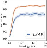
(a) training, diff $0.4$

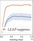
(b) OOD, diff $0.25$

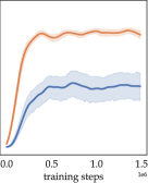
(c) OOD, diff $0.35$

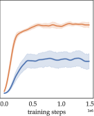
(d) OOD, diff $0.45$

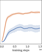
(e) OOD, diff $0.55$

Figure 26: Comparative Results of LEAP with and without the delusion suppression technique: the results are obtained with $50$ training tasks. The results are obtained from $20$ independent seed runs.

Appendix G Director Implementation Details

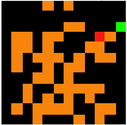
Figure 27: An example for simplified observations for Director.

Adaptation. For our experiments with Director (Hafner et al., 2022), we have used the publicly available code provided by the authors. Except for a few changes in the parameters, which are depicted in Table 3, we have used the default configuration provided for Atari environments. Note that as the Director version in which the worker receives no task rewards performed very badly in our environment, we have used the version in which the worker receives scaled task rewards (referred to as “Director (worker task reward)” in Hafner et al. (2022)). This agent has also been shown to perform better across various domains in Hafner et al. (2022).

Encoder. Unlike Skipper and LEAP agents, the Director agent receives as input a simplified RGB image of the current state of the environment (see Fig. 27). This is because we found that Director performed better with its original architecture, which was designed for image-based observations. To simplify the representation learning of Director as much as possible, we also used a simplified RGB image, instead of a detailed one (where the lava cells have waves on top etc.).

Table 3: The changed parameters and their values in the config file of the Director agent.

Parameter	Value
replay_size	2M
replay_chunk	12
imag_horizon	8
env_skill_duration	4
train_skill_duration	4
worker_rews	{extr: 0.5, expl: 0.0, goal: 1.0}
sticky	False
gray	False

Training Performance. We investigated why Director is unable to achieve near optimal training performance in the used environment (Fig. 3). As Director was trained solely on environments where it is able to collect long trajectories to train a good enough recurrent world model (Hafner et al., 2022), we hypothesized that Director may perform better in domains where it is able to interact with the environment through longs trajectories to train a good enough recurrent world model (i.e., the agent does not immediately die as a result of interacting with specific objects in the environment). To test this, we experimented with variants of the used environments, where the lava cells are replaced with wall cells, so the agent does not die upon trying to move towards them (we refer to this environment as the “walled” environment). The corresponding results on $50$ training tasks are depicted in Fig. 28. As can be seen, the Director agent indeed performs better within the training tasks than in the environments with lava.

Generalization Performance. We also investigated why Director is unable to achieve good generalization performance in the used environment (Fig. 3). As Director trains its policies solely from the imagined trajectories predicted by its learned world model, we believe that the low generalization performance is due to Director being unable to learn a good enough world model that generalizes to the evaluation tasks. The generalization performances in both the “walled” and regular environments, depicted in Fig. 28, indeed support this argument. Similar to the main paper, we also present experimental results for how the generalization performance changes with the number of training environments that are used. Results in Fig. 29 show that the number of training environments has no effect on the poor generalization performance of Director.

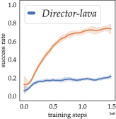
(a) training, diff $0.4$

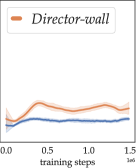
(b) OOD, diff $0.25$

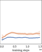
(c) OOD, diff $0.35$

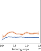
(d) OOD, diff $0.45$

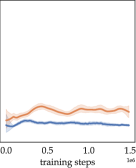
(e) OOD, diff $0.55$

Figure 28: Comparative Results of Director on Environments with Lavas and on those with Walls: the results are obtained with $50$ training tasks. The results for Director-lava (same as in the main paper) are obtained from $20$ independent seed runs.

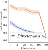
(a) training, diff $0.4$

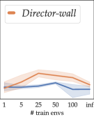
(b) OOD, diff $0.25$

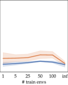
(c) OOD, diff $0.35$

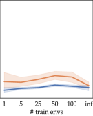
(d) OOD, diff $0.45$

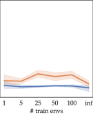
(e) OOD, diff $0.55$

Figure 29: Generalization Performance of Agents on Different Numbers of Training Tasks (while Director runs on the walled environments): besides Director, each data point and corresponding error bar (95% confidence interval) are processed from the final performance from $20$ independent seed runs. Director-wall’s results are obtained from $20$ runs.

Appendix H Pseudo Code (with Hyper-Parameters)

H.1 Overall Skipper Framework

The pseudocode of Skipper is provided in Alg. 2.

H.2 k-medoids based pruning

for each episode do

       //construct the proxy problem, can be done multiple times in one episode too (as in Skipper-regen)

      

      generate more than necessary (32) checkpoints by sampling from the partial description latent space given the extracted context from the initial state

      

      k-medoid pruning based on the distance estimations among all checkpoints (down to $12$ vertices)

      

      use estimators to construct the pruned graph (including a terminal state estimator to correct the estimates)

      

      prune edges that are too far-fetched according to distance estimations (threshold set to be $8$, same as replan interval)

      

      for each agent-environment interaction step do

             if decided to explore (DQN-style annealing $\epsilon$-greedy) then

                   take a random action

                  

            else

                   if abstract problem just constructed or a checkpoint / timeout reached ($\geq 8$ steps since last planned) then

                         run value iteration (for $5$ iterations) on the proxy problem, select the target checkpoint

                        

                  follow the action suggested by the checkpoint-achieving policy

                  

            if time to train (every $4$ actions) then

                   sample hindsight transitions and train checkpoint-achieving policy, estimators (including a teriminal state estimator) and checkpoint generator

                  

                  [optional delusion control]: generate imaginary states and use them to train the estimators

                  

            save interaction into the trajectory experience replay

            

      convert trajectory into hindsight samples in HER (relabel $4$ random states as additional goals)

      

Algorithm 2 Skipper with Random Checkpoints (implementation choice in purple)

We present the pseudocode of the modified $k$-medoids algorithm for pruning overcrowded checkpoints in Alg. 3. Note that the actual implementation is parallelized, the simplification for presentation is intended for reader’s understanding. The changes upon the original $k$-medoids algorithm is marked in purple. When $k$-medoids is called after the unpruned graph is constructed, $\mathcal{S}_{\vee}$ is set to be the set containing the goal state only. This is intended to span more uniformly in the state space with checkpoints, taking consideration into the goal. Let the estimated distance matrix be $D$, where each element $d_{i}j$ represents the estimated trajectory length it takes for $\pi$ to fulfill the transition from checkpoint $i$ to checkpoint $j$. Since $k$-medoids cannot handle infinite distances (e.g. from a terminal state to another state), the distance matrix $D$ is truncated, and then we take the elementwise minimum between the truncated $D$ and $D^{T}$ to preserve the one-way distances. The matrix containing the elementwise minimums would be the input of the pruning algorithm.

Data: $X=\{x_{1},x_{2},\ldots,x_{n}\}$ (state indices), $D$ (estimated distance matrix), $\mathcal{S}_{\vee}$ (states that must be kept), $k$ (#checkpoints to keep)

Result: $\mathcal{S}_{\odot}\equiv\{M_{1},M_{2},\ldots,M_{k}\}$ (checkpoints kept)

Initialize $\mathcal{S}_{\odot}\equiv\{M_{1},M_{2},\ldots,M_{k}\}$ randomly from $X$

make sure $\mathcal{S}_{\vee}\subset\mathcal{S}_{\odot}$

repeat

       Assign each data point $x_{i}$ to the nearest medoid $M_{j}$, forming clusters $C_{1},C_{2},\ldots,C_{k}$;

       foreach medoid $M_{j}$ do

             Calculate the cost $J_{j}$ of $M_{j}$ as the sum of distances between $M_{j}$ and the data points in $C_{j}$;

            

      Find the medoid $M_{j}$ with the lowest cost $J_{j}$;

       if $M_{j}$ changes then

             make sure $\mathcal{S}_{\vee}\subset\mathcal{S}_{\odot}$

             Replace $M_{j}$ with the data point in $C_{j}$ that minimizes the total cost;

            

      

until Convergence (no cost improvement);

Algorithm 3 Checkpoint Pruning with $k$-medoids

Appendix I Weaknesses and Limitations

We would like to discuss the limitations to the current form of the framework, as well as the design choices that we seek to improve in the future:

• We generate future checkpoints at random by sampling the partial description space. Despite the post-processing such as pruning, the generated checkpoints do not prioritize on the predictable, important states that matter the most to form a meaningful long-term plan. We would like to continue investigating the possibilities along this line;

• The current implementation is intended for pixel input fully-observable tasks with discrete state and action spaces. Such a minimalistic form is because we wish to isolate the unwanted challenges from other factors that are not closely related to the idea of this work, as well as to make the agent as generalist as possible. On the matter of the compatibility with continuous spaces, Skipper is naturally compatible with continuous actions spaces and the only thing we will need to do is to replace the baseline agent with a compatible one such as TD3 (Fujimoto et al., 2018); on the other hand, for continuous state spaces, the identification of the achievement of a checkpoint becomes tricky. This is due to the fact that a strict identity between the current state and the target checkpoint may be ever established, we either must adopt a distance measure for approximate state equivalence, or rely on the equivalence of the partial descriptions (which is adopted in the current implementation). We intentionally designed the partial descriptions to be in the form of bundles of binary variables, so that this comparison could be done fast and trivially for any forms of the state space; for partial observability, despite that no recurrent mechanism has been incorporated in the current implementation, the framework is not incompatible. To implement that, we will need to augment the state encoder with recurrent or memory mechanisms and we need to make the checkpoint generator directly work over the learned state representations. We acknowledge that future work is needed to verify Skipper’s performance on the popular partially-observable benchmark suites, which requires the incorporation of components to handle partial observability as well as scaling up the architectures for more expressive power;

• We are far from understanding the precise boundaries of the motivating theory on proxy problems, since it only indicates performance guarantees on the condition of estimation accuracy, which in turn does not correspond trivially to a set of well-defined problems. We are eager to explore, outside the scope of sparse-reward navigation, how this approach can be used to facilitate better generalization, and at the same time, try to find more powerful theories that guide us better;

Appendix J Theoretical Analyses

J.1 Update Rules for Edge Estimation

First, we show that the update rules proposed in the main paper indeed estimate the desired cumulative discount and reward.

The low-level checkpoint-achieving policy $\pi$ is trained with an intrinsic reward to reach target state $s^{\odot}$. The cumulative reward and cumulative discount are estimated by applying policy evaluation given $\pi$, on the two sets of auxiliary reward signals, respectively.

For the cumulative discounted reward random variable:

$$V_{\pi}(s_{t},a_{t}|s^{\odot}) =R(s_{t},a_{t},S_{t+1})+\gamma V_{\pi}(S_{t+1},A_{t+1}|s^{\odot})$$ (5)

$$=\sum_{\tau=t}^{\infty}\gamma^{\tau-t}R(S_{\tau},A_{\tau},S_{\tau+1}),$$ (6)

where $S_{t+1}\sim p(\cdot|s_{t},a_{t})$, $A_{t+1}\sim\pi(\cdot|S_{t+1},s^{\odot})$, and with $V_{\pi}(S_{t+1},A_{t+1}|s^{\odot})=0$ if $S_{t+1}=s^{\odot}$. We overload the notation as follows: $V_{\pi}(s|s^{\odot})\doteq V_{\pi}(s,A|s^{\odot})$ with $A\sim\pi(\cdot|s,s^{\odot})$.

The cumulative discount random variable denotes the event that the trajectory did not terminate before reaching the target $s^{\odot}$:

$$\Gamma_{\pi}(S_{t},A_{t}|s^{\odot}) =\gamma\cdot\Gamma_{\pi}(S_{t+1},A_{t+1}|s^{\odot}),$$ (7)

$$=\gamma^{T_{\perp}-t}\mathbb{I}{\{S_{T_{\perp}}=s^{\odot}\}},$$ (8)

where $T_{\perp}$ denotes the timestep when the trajectory terminates, and with $\Gamma_{\pi}(S_{t+1},A_{t+1}|s^{\odot})=1$ if $S_{t+1}=s^{\odot}$ and $\Gamma_{\pi}(S_{t+1},A_{t+1}|s^{\odot})=0$ if $S_{t+1}\neq s^{\odot}$ is terminal. We overload the notation as follows: $\Gamma_{\pi}(s_{t}|s^{\odot})\doteq\Gamma_{\pi}(s_{t},A_{t}|s^{\odot})$ with $A_{t+1}\sim\pi(\cdot|S_{t+1},s^{\odot})$.

Note that, for the sake of simplicity, we take here the view that the terminality of states is deterministic, but this is not reductive as any state with a stochastic terminality can be split into two identical states: one that is deterministically non-terminal and the other that is deterministically terminal. Note also that we could adopt the view that the discount factor is the constant probability of the trajectory to not terminate.

J.2 Performance Bound

We are going to denote the expected cumulative discounted reward, a.k.a. the state-action value with $q_{\pi}\doteq\mathbb{E}_{\pi}[V]$, and let $\hat{q}_{\pi}$ be our estimate for it. We are also going to consider the state value $v_{\pi}(s|s^{\odot})\doteq\sum_{a}\pi(a|s,s^{\odot})q_{\pi}(s,a|s^{\odot})$ and its estimate $\hat{v}_{\pi}$. Similarly, we denote the expected cumulative discount with $\gamma_{\pi}\doteq\mathbb{E}_{\pi}[\Gamma]$ and its estimate with $\hat{\gamma}_{\pi}$.

We are in the presence of a hierarchical policy. The high level policy $\mu$ consists in (potentially) stochastically picking a sequence of checkpoints. The low-level policy is implemented by $\pi$ which is assumed to be given and fixed for the moment. The composite policy $\mu\circ\pi$ is non-Markovian: it depends both on the current state and the current checkpoint goal. So there is no notion of state value, except when we arrive at a checkpoint, i.e. when a high level action (checkpoint selection) needs to be chosen.

Proceeding further, we adopt the view where the discounts are a way to represent the hazard of the environment: $1-\gamma$ is the probability of sudden trajectory termination. In this view, $v_{\pi}$ denotes the (undiscounted: there is no more discounting) expected sum of reward before reaching the next checkpoint, and more interestingly $\gamma_{\pi}$ denotes the binomial random variable of non-termination during the transition to the selected checkpoint.

Making the following assumption that the trajectory terminates almost surely when reaching the goal, i.e. $\gamma_{\pi}(s_{i},s_{g})=0,\forall s_{i}$, the gain $V$ can be written:

$$V_{0}=V(S_{0}^{\odot}|S_{1}^{\odot})+\Gamma(S_{0}^{\odot}|S_{1}^{\odot})V_{1}=\sum_{k=0}^{\infty}V(S_{k}^{\odot}|S_{k+1}^{\odot})\prod_{i=0}^{k-1}\Gamma(S_{i}^{\odot}|S_{i+1}^{\odot}),$$ (9)

where $S_{k+1}\sim\mu(\cdot|S_{k})$, where $V(S_{k}^{\odot}|S_{k+1}^{\odot})$ is the gain obtained during the path between $S_{k}^{\odot}$ and where $S_{k+1}^{\odot}$, and $\Gamma(S_{k}^{\odot}|S_{k+1}^{\odot})$ is either 0 or 1 depending whether the trajectory terminated or reached $S_{k+1}^{\odot}$. If we consider $\mu$ as a deterministic planning routine over the checkpoints, then the action space of $\mu$ boils down to a list of checkpoints $\{s^{\odot}_{0}=s_{0},s^{\odot}_{1},\cdots,s^{\odot}_{n}=s_{g}\}$. Thanks to the Markovian property in checkpoints, we have independence between $V_{\pi}$ and $\Gamma_{\pi}$, therefore for the expected value of $\mu\circ\pi$, we have:

$$v_{\mu\circ\pi}(s_{0})\doteq\mathbb{E}_{\mu\circ\pi}[V|S_{0}=s_{0}]=\sum_{k=0}^{\infty}v_{\pi}(s^{\odot}_{k}|s^{\odot}_{k+1})\prod_{i=0}^{k-1}\gamma_{\pi}(s^{\odot}_{i}|s^{\odot}_{i+1})$$ (10)

Having obtained the ground truth value, in the following, we are going to consider the estimates which may have small error terms:

$$|v_{\pi}(s)-\hat{v}_{\pi}(s)|<\epsilon_{v}v_{\text{max}}\ll(1-\gamma)v_{\text{max}}\quad\quad\text{and}\quad\quad|\gamma_{\pi}(s)-\hat{\gamma}_{\pi}(s)|<\epsilon_{\gamma}\ll(1-\gamma)^{2}\quad\quad\forall s.$$ (11)

We are looking for a performance bound, and assume without loss of generality that the reward function is non-negative, s.t. the values are guaranteed to be non-negative as well. We provide an upper bound:

$$\ \hat{v}_{\mu\circ\pi}(s)\doteq\sum_{k=0}^{\infty}\hat{v}_{\pi}(s^{\odot}_{k}|s^{\odot}_{k+1})\prod_{i=0}^{k-1}\hat{\gamma}_{\pi}(s^{\odot}_{i}|s^{\odot}_{i+1})$$ (12)

$$\leq\sum_{k=0}^{\infty}\left(v_{\pi}(s^{\odot}_{k}|s^{\odot}_{k+1})+\epsilon_{v}v_{\text{max}}\right)\prod_{i=0}^{k-1}\left(\gamma_{\pi}(s^{\odot}_{i}|s^{\odot}_{i+1})+\epsilon_{\gamma}\right)$$ (13)

$$\leq v_{\mu\circ\pi}(s)+\sum_{k=0}^{\infty}\epsilon_{v}v_{\text{max}}\prod_{i=0}^{k-1}\left(\gamma_{\pi}(s^{\odot}_{i}|s^{\odot}_{i+1})+\epsilon_{\gamma}\right)+\sum_{k=0}^{\infty}\left(v_{\pi}(s^{\odot}_{k}|s^{\odot}_{k+1})+\epsilon_{v}v_{\text{max}}\right)k\epsilon_{\gamma}\gamma^{k}+o(\epsilon_{v}+\epsilon_{\gamma})$$ (14)

$$\leq v_{\mu\circ\pi}(s)+\epsilon_{v}v_{\text{max}}\sum_{k=0}^{\infty}\gamma^{k}+\epsilon_{\gamma}v_{\text{max}}\sum_{k=0}^{\infty}k\gamma^{k}+o(\epsilon_{v}+\epsilon_{\gamma})$$ (15)

$$\leq v_{\mu\circ\pi}(s)+\frac{\epsilon_{v}v_{\text{max}}}{1-\gamma}+\frac{\epsilon_{\gamma}v_{\text{max}}}{(1-\gamma)^{2}}+o(\epsilon_{v}+\epsilon_{\gamma})$$ (16)

Similarly, we can derive a lower bound:

$$\ \hat{v}_{\mu\circ\pi}(s)\doteq\sum_{k=0}^{\infty}\hat{v}_{\pi}(s^{\odot}_{k}|s^{\odot}_{k+1})\prod_{i=0}^{k-1}\hat{\gamma}_{\pi}(s^{\odot}_{i}|s^{\odot}_{i+1})$$ (17)

$$\geq\sum_{k=0}^{\infty}\left(v_{\pi}(s^{\odot}_{k}|s^{\odot}_{k+1})-\epsilon_{v}v_{\text{max}}\right)\prod_{i=0}^{k-1}\left(\gamma_{\pi}(s^{\odot}_{i}|s^{\odot}_{i+1})-\epsilon_{\gamma}\right)$$ (18)

$$\geq v_{\mu\circ\pi}(s)-\sum_{k=0}^{\infty}\epsilon_{v}v_{\text{max}}\prod_{i=0}^{k-1}\left(\gamma_{\pi}(s^{\odot}_{i}|s^{\odot}_{i+1})-\epsilon_{\gamma}\right)-\sum_{k=0}^{\infty}\left(v_{\pi}(s^{\odot}_{k}|s^{\odot}_{k+1})-\epsilon_{v}v_{\text{max}}\right)k\epsilon_{\gamma}\gamma^{k}+o(\epsilon_{v}+\epsilon_{\gamma})$$ (19)

$$\geq v_{\mu\circ\pi}(s)-\epsilon_{v}v_{\text{max}}\sum_{k=0}^{\infty}\gamma^{k}-\epsilon_{\gamma}v_{\text{max}}\sum_{k=0}^{\infty}k\gamma^{k}+o(\epsilon_{v}+\epsilon_{\gamma})$$ (20)

$$\geq v_{\mu\circ\pi}(s)-\frac{\epsilon_{v}v_{\text{max}}}{1-\gamma}-\frac{\epsilon_{\gamma}v_{\text{max}}}{(1-\gamma)^{2}}+o(\epsilon_{v}+\epsilon_{\gamma})$$ (21)

We may therefore conclude that $\hat{v}_{\mu\circ\pi}$ equals $v_{\mu\circ\pi}$ up to an accuracy of $\frac{\epsilon_{v}v_{\text{max}}}{1-\gamma}+\frac{\epsilon_{\gamma}v_{\text{max}}}{(1-\gamma)^{2}}+o(\epsilon_{v}+\epsilon_{\gamma})$. Note that the requirement for the reward function to be positive is only a cheap technical trick to ensure we bound in the right direction of $\epsilon_{\gamma}$ errors in the discounting, but that the theorem would still stand if it were not the case.

J.3 No Assumption on Optimality

If the low-level policy $\pi$ is perfect, then the best high-level policy $\mu$ is to choose directly the goal as target. Our approach assumes that it would be difficult to learn effectively a $\pi$ when the target is too far, and that we would rather use a proxy to construct a path with shorter-distance transitions. Therefore, we’ll never want to make any optimality assumption on $\pi$, otherwise our approach is pointless. These theories we have initiated makes no assumption on $\pi$.

The Theorem provides guarantees on the solution to the overall problem. The quality of the solution depends on both the quality of the estimates (distances/discounts, rewards) and the quality of the policy, as the theorem guarantees accuracy to the solution of the overall problem given a current policy, which should evolve towards optimal during training. This means bad policy with good estimation will lead to an accurate yet bad overall solution. No matter the quality of the policy, with a bad estimation, it will result in a poor estimate of solutions. Only a near-optimal policy and good estimation will lead to a near-optimal solution.

References

- Alver & Precup (2022) Safa Alver and Doina Precup. Understanding decision-time vs. background planning in model-based reinforcement learning. arXiv preprint arXiv:2206.08442, 2022.
- Alver & Precup (2023) Safa Alver and Doina Precup. Minimal value-equivalent partial models for scalable and robust planning in lifelong reinforcement learning. arXiv preprint arXiv:2301.10119, 2023.
- Andrychowicz et al. (2017) Marcin Andrychowicz, Filip Wolski, Alex Ray, Jonas Schneider, Rachel Fong, Peter Welinder, Bob McGrew, Josh Tobin, OpenAI Pieter Abbeel, and Wojciech Zaremba. Hindsight experience replay. Advances in neural information processing systems, 30, 2017.
- Ba et al. (2016) Jimmy Lei Ba, Jamie Ryan Kiros, and Geoffrey E Hinton. Layer normalization. arXiv preprint arXiv:1607.06450, 2016.
- Bacon et al. (2017) Pierre-Luc Bacon, Jean Harb, and Doina Precup. The option-critic architecture. In Proceedings of the AAAI conference on artificial intelligence, volume 31, 2017.
- Bagaria et al. (2021) Akhil Bagaria, Jason K Senthil, and George Konidaris. Skill discovery for exploration and planning using deep skill graphs. In International Conference on Machine Learning, pp. 521–531. PMLR, 2021.
- Bengio (2017) Yoshua Bengio. The consciousness prior. arXiv, 1709.08568, 2017. http://arxiv.org/abs/1709.08568.
- Bengio et al. (2013) Yoshua Bengio, Nicholas Léonard, and Aaron Courville. Estimating or propagating gradients through stochastic neurons for conditional computation. arXiv preprint:1308.3432, 2013.
- Chevalier-Boisvert et al. (2018a) Maxime Chevalier-Boisvert, Dzmitry Bahdanau, Salem Lahlou, Lucas Willems, Chitwan Saharia, Thien Huu Nguyen, and Yoshua Bengio. Babyai: A platform to study the sample efficiency of grounded language learning. International Conference on Learning Representations, 2018a. http://arxiv.org/abs/1810.08272.
- Chevalier-Boisvert et al. (2018b) Maxime Chevalier-Boisvert, Lucas Willems, and Suman Pal. Minimalistic gridworld environment for openai gym. GitHub repository, 2018b. https://github.com/maximecb/gym-minigrid.
- Cobbe et al. (2020) Karl Cobbe, Chris Hesse, Jacob Hilton, and John Schulman. Leveraging procedural generation to benchmark reinforcement learning. In International conference on machine learning, pp. 2048–2056. PMLR, 2020.
- Colas et al. (2018) Cédric Colas, Olivier Sigaud, and Pierre-Yves Oudeyer. How many random seeds? statistical power analysis in deep reinforcement learning experiments, 2018.
- Şimşek & Barto (2004) Özgür Şimşek and Andrew G. Barto. Using relative novelty to identify useful temporal abstractions in reinforcement learning. In Proceedings of the Twenty-First International Conference on Machine Learning, ICML ’04, pp. 95, New York, NY, USA, 2004. Association for Computing Machinery. ISBN 1581138385. URL https://doi.org/10.1145/1015330.1015353.
- Czechowski et al. (2021) Konrad Czechowski, Tomasz Odrzygóźdź, Marek Zbysiński, Michał Zawalski, Krzysztof Olejnik, Yuhuai Wu, Łukasz Kuciński, and Piotr Miłoś. Subgoal search for complex reasoning tasks. arXiv preprint:2108.11204, 2021.
- Dabney et al. (2018) Will Dabney, Mark Rowland, Marc Bellemare, and Rémi Munos. Distributional reinforcement learning with quantile regression. In Proceedings of the AAAI Conference on Artificial Intelligence, volume 32, 2018.
- Dehaene et al. (2020) Stanislas Dehaene, Hakwan Lau, and Sid Kouider. What is consciousness, and could machines have it? Science, 358, 2020. URL https://science.sciencemag.org/content/358/6362/486.
- Dietterich (2000) Thomas G Dietterich. Hierarchical reinforcement learning with the maxq value function decomposition. Journal of artificial intelligence research, 13:227–303, 2000.
- Erraqabi et al. (2021) Akram Erraqabi, Mingde Zhao, Marlos C Machado, Yoshua Bengio, Sainbayar Sukhbaatar, Ludovic Denoyer, and Alessandro Lazaric. Exploration-driven representation learning in reinforcement learning. In ICML 2021 Workshop on Unsupervised Reinforcement Learning, 2021.
- Eysenbach et al. (2019) Ben Eysenbach, Russ R Salakhutdinov, and Sergey Levine. Search on the replay buffer: Bridging planning and reinforcement learning. In H. Wallach, H. Larochelle, A. Beygelzimer, F. d'Alché-Buc, E. Fox, and R. Garnett (eds.), Advances in Neural Information Processing Systems, volume 32. Curran Associates, Inc., 2019. URL https://proceedings.neurips.cc/paper_files/paper/2019/file/5c48ff18e0a47baaf81d8b8ea51eec92-Paper.pdf.
- Florensa et al. (2018) Carlos Florensa, David Held, Xinyang Geng, and Pieter Abbeel. Automatic goal generation for reinforcement learning agents. In International conference on machine learning, pp. 1515–1528. PMLR, 2018.
- Fu et al. (2021) Xiang Fu, Ge Yang, Pulkit Agrawal, and Tommi Jaakkola. Learning task informed abstractions. In International Conference on Machine Learning, pp. 3480–3491. PMLR, 2021.
- Fujimoto et al. (2018) Scott Fujimoto, Herke van Hoof, and David Meger. Addressing function approximation error in actor-critic methods, 2018.
- Gupta et al. (2021) Ankit Gupta, Guy Dar, Shaya Goodman, David Ciprut, and Jonathan Berant. Memory-efficient transformers via top- attention. arXiv preprint:2106.06899, 2021.
- Hafner et al. (2019) Danijar Hafner, Timothy Lillicrap, Ian Fischer, Ruben Villegas, David Ha, Honglak Lee, and James Davidson. Learning latent dynamics for planning from pixels. In International conference on machine learning, pp. 2555–2565. PMLR, 2019.
- Hafner et al. (2022) Danijar Hafner, Kuang-Huei Lee, Ian Fischer, and Pieter Abbeel. Deep hierarchical planning from pixels. In Alice H. Oh, Alekh Agarwal, Danielle Belgrave, and Kyunghyun Cho (eds.), Advances in Neural Information Processing Systems, 2022. URL https://openreview.net/forum?id=wZk69kjy9_d.
- Hafner et al. (2023) Danijar Hafner, Jurgis Pasukonis, Jimmy Ba, and Timothy Lillicrap. Mastering diverse domains through world models. arXiv preprint:2301.04104, 2023.
- Hogg et al. (2009) Chad Hogg, Ugur Kuter, and Héctor Muñoz Avila. Learning hierarchical task networks for nondeterministic planning domains. In Proceedings of the 21st International Joint Conference on Artificial Intelligence, IJCAI’09, pp. 1708–1714, San Francisco, CA, USA, 2009. Morgan Kaufmann Publishers Inc.
- Hui et al. (2020) David Yu-Tung Hui, Maxime Chevalier-Boisvert, Dzmitry Bahdanau, and Yoshua Bengio. Babyai 1.1, 2020.
- Igl et al. (2019) Maximilian Igl, Kamil Ciosek, Yingzhen Li, Sebastian Tschiatschek, Cheng Zhang, Sam Devlin, and Katja Hofmann. Generalization in reinforcement learning with selective noise injection and information bottleneck. Advances in neural information processing systems, 32, 2019.
- Kahneman (2017) Daniel Kahneman. Thinking, fast and slow. 2017.
- Kaufman & Rousseeuw (1990) Leonard Kaufman and Peter Rousseeuw. Partitioning Around Medoids (Program PAM), chapter 2, pp. 68–125. John Wiley & Sons, Ltd, 1990. URL https://onlinelibrary.wiley.com/doi/abs/10.1002/9780470316801.ch2.
- Kim et al. (2021) Junsu Kim, Younggyo Seo, and Jinwoo Shin. Landmark-guided subgoal generation in hierarchical reinforcement learning. arXiv preprint:2110.13625, 2021.
- Kingma & Ba (2014) Diederik P Kingma and Jimmy Ba. Adam: A method for stochastic optimization. arXiv preprint:1412.6980, 2014.
- Knoblock (1994) Craig A Knoblock. Automatically generating abstractions for planning. Artificial intelligence, 68(2):243–302, 1994.
- Konidaris & Barto (2009) George Dimitri Konidaris and Andrew G Barto. Efficient skill learning using abstraction selection. In IJCAI, volume 9, pp. 1107–1112, 2009.
- Kulkarni et al. (2016) Tejas D Kulkarni, Karthik Narasimhan, Ardavan Saeedi, and Josh Tenenbaum. Hierarchical deep reinforcement learning: Integrating temporal abstraction and intrinsic motivation. Advances in neural information processing systems, 29, 2016.
- Langosco et al. (2022) Lauro Langosco Di Langosco, Jack Koch, Lee D Sharkey, Jacob Pfau, and David Krueger. Goal misgeneralization in deep reinforcement learning. In International Conference on Machine Learning, volume 162, pp. 12004–12019, 17-23 Jul 2022. URL https://proceedings.mlr.press/v162/langosco22a.html.
- Li et al. (2006) Lihong Li, Thomas J Walsh, and Michael L Littman. Towards a unified theory of state abstraction for mdps. AI&M, 1(2):3, 2006.
- Manchin et al. (2019) Anthony Manchin, Ehsan Abbasnejad, and Anton Van Den Hengel. Reinforcement learning with attention that works: A self-supervised approach. In Neural Information Processing: 26th International Conference, ICONIP 2019, Sydney, NSW, Australia, December 12–15, 2019, Proceedings, Part V 26, pp. 223–230. Springer, 2019.
- McGovern & Barto (2001) Amy McGovern and Andrew G Barto. Automatic discovery of subgoals in reinforcement learning using diverse density. 2001.
- Momennejad et al. (2017) Ida Momennejad, Evan M Russek, Jin H Cheong, Matthew M Botvinick, Nathaniel Douglass Daw, and Samuel J Gershman. The successor representation in human reinforcement learning. Nature human behaviour, 1(9):680–692, 2017.
- Mott et al. (2019) Alexander Mott, Daniel Zoran, Mike Chrzanowski, Daan Wierstra, and Danilo Jimenez Rezende. Towards interpretable reinforcement learning using attention augmented agents. Advances in neural information processing systems, 32, 2019.
- Nachum et al. (2018) Ofir Nachum, Shixiang Shane Gu, Honglak Lee, and Sergey Levine. Data-efficient hierarchical reinforcement learning. Advances in neural information processing systems, 31, 2018.
- Nair et al. (2018) Ashvin Nair, Vitchyr Pong, Murtaza Dalal, Shikhar Bahl, Steven Lin, and Sergey Levine. Visual reinforcement learning with imagined goals. arXiv preprint:1807.04742, 2018.
- Nair & Finn (2020) Suraj Nair and Chelsea Finn. Hierarchical foresight: Self-supervised learning of long-horizon tasks via visual subgoal generation. In International Conference on Learning Representations, 2020. URL https://openreview.net/forum?id=H1gzR2VKDH.
- Nasiriany et al. (2019) Soroush Nasiriany, Vitchyr Pong, Steven Lin, and Sergey Levine. Planning with goal-conditioned policies. Advances in Neural Information Processing Systems, 32, 2019.
- Paolo et al. (2022) Giuseppe Paolo, Jonas Gonzalez-Billandon, Albert Thomas, and Balázs Kégl. Guided safe shooting: model based reinforcement learning with safety constraints, 2022.
- Patterson et al. (2023) Andrew Patterson, Samuel Neumann, Martha White, and Adam White. Empirical design in reinforcement learning, 2023.
- Pong et al. (2018) Vitchyr Pong, Shixiang Gu, Murtaza Dalal, and Sergey Levine. Temporal difference models: Model-free deep rl for model-based control. arXiv preprint:1802.09081, 2018.
- Puterman (2014) Martin L Puterman. Markov decision processes: discrete stochastic dynamic programming. John Wiley & Sons, 2014.
- Rubinstein (1997a) Reuven Y. Rubinstein. Optimization of computer simulation models with rare events. European Journal of Operational Research, 99(1):89–112, 1997a. ISSN 0377-2217. doi: https://doi.org/10.1016/S0377-2217(96)00385-2. URL https://www.sciencedirect.com/science/article/pii/S0377221796003852.
- Rubinstein (1997b) Reuven Y Rubinstein. Optimization of computer simulation models with rare events. European Journal of Operational Research, 99(1):89–112, 1997b.
- Sacerdoti (1974) Earl D Sacerdoti. Planning in a hierarchy of abstraction spaces. Artificial intelligence, 5(2):115–135, 1974.
- Savinov et al. (2018) Nikolay Savinov, Alexey Dosovitskiy, and Vladlen Koltun. Semi-parametric topological memory for navigation. arXiv preprint arXiv:1803.00653, 2018.
- Schrittwieser et al. (2020) Julian Schrittwieser, Ioannis Antonoglou, Thomas Hubert, Karen Simonyan, Laurent Sifre, Simon Schmitt, Arthur Guez, Edward Lockhart, Demis Hassabis, Thore Graepel, et al. Mastering atari, go, chess and shogi by planning with a learned model. Nature, 588(7839):604–609, 2020.
- Shah et al. (2021) Dhruv Shah, Peng Xu, Yao Lu, Ted Xiao, Alexander Toshev, Sergey Levine, and Brian Ichter. Value function spaces: Skill-centric state abstractions for long-horizon reasoning. arXiv preprint arXiv:2111.03189, 2021.
- Sharma et al. (2019) Archit Sharma, Shixiang Gu, Sergey Levine, Vikash Kumar, and Karol Hausman. Dynamics-aware unsupervised discovery of skills. arXiv preprint arXiv:1907.01657, 2019.
- Shi et al. (2022) Lucy Xiaoyang Shi, Joseph J Lim, and Youngwoon Lee. Skill-based model-based reinforcement learning. arXiv preprint arXiv:2207.07560, 2022.
- Silver & Ciosek (2012) David Silver and Kamil Ciosek. Compositional planning using optimal option models. arXiv preprint arXiv:1206.6473, 2012.
- Silver et al. (2017) David Silver, Julian Schrittwieser, Karen Simonyan, Ioannis Antonoglou, Aja Huang, Arthur Guez, Thomas Hubert, Lucas Baker, Matthew Lai, Adrian Bolton, et al. Mastering the game of go without human knowledge. Nature, 550(7676):354–359, 2017.
- Sohn et al. (2015) Kihyuk Sohn, Honglak Lee, and Xinchen Yan. Learning structured output representation using deep conditional generative models. In C. Cortes, N. Lawrence, D. Lee, M. Sugiyama, and R. Garnett (eds.), Neural Information Processing Systems, volume 28. Curran Associates, Inc., 2015. URL https://proceedings.neurips.cc/paper_files/paper/2015/file/8d55a249e6baa5c06772297520da2051-Paper.pdf.
- Sutton (1991) Richard S. Sutton. Dyna, an integrated architecture for learning, planning, and reacting. SIGART Bulletin, 2(4):160–163, 1991. URL https://bit.ly/3jIyN5D.
- Sutton et al. (1999) Richard S. Sutton, Doina Precup, and Satinder Singh. Between mdps and semi-mdps: A framework for temporal abstraction in reinforcement learning. Artificial Intelligence, 112(1):181–211, 1999. URL https://bit.ly/3jKkJrY.
- Sutton et al. (2022) Richard S Sutton, Marlos C Machado, G Zacharias Holland, David Szepesvari Finbarr Timbers, Brian Tanner, and Adam White. Reward-respecting subtasks for model-based reinforcement learning. arXiv preprint:2202.03466, 2022.
- Sylvain et al. (2019) Tristan Sylvain, Linda Petrini, and Devon Hjelm. Locality and compositionality in zero-shot learning. arXiv preprint arXiv:1912.12179, 2019.
- Tang & Salakhutdinov (2019) Charlie Tang and Russ R Salakhutdinov. Multiple futures prediction. Advances in neural information processing systems, 32, 2019.
- Tang et al. (2020) Yujin Tang, Duong Nguyen, and David Ha. Neuroevolution of self-interpretable agents. In Proceedings of the 2020 Genetic and Evolutionary Computation Conference, pp. 414–424, 2020.
- Van Den Oord et al. (2017) Aaron Van Den Oord, Oriol Vinyals, et al. Neural discrete representation learning. Advances in neural information processing systems, 30, 2017.
- Van Hasselt et al. (2016) Hado Van Hasselt, Arthur Guez, and David Silver. Deep reinforcement learning with double q-learning. In Proceedings of the AAAI conference on artificial intelligence, volume 30, 2016.
- Xie et al. (2020) Kevin Xie, Homanga Bharadhwaj, Danijar Hafner, Animesh Garg, and Florian Shkurti. Latent skill planning for exploration and transfer. arXiv preprint arXiv:2011.13897, 2020.
- Zadaianchuk et al. (2020) Andrii Zadaianchuk, Maximilian Seitzer, and Georg Martius. Self-supervised visual reinforcement learning with object-centric representations. arXiv preprint arXiv:2011.14381, 2020.
- Zhang et al. (2020) Amy Zhang, Clare Lyle, Shagun Sodhani, Angelos Filos, Marta Kwiatkowska, Joelle Pineau, Yarin Gal, and Doina Precup. Invariant causal prediction for block mdps. In International Conference on Machine Learning, pp. 11214–11224. PMLR, 2020.
- Zhang et al. (2021) Lunjun Zhang, Ge Yang, and Bradly C Stadie. World model as a graph: Learning latent landmarks for planning. In International Conference on Machine Learning, pp. 12611–12620. PMLR, 2021.
- Zhao et al. (2019) Mingde Zhao, Sitao Luan, Ian Porada, Xiao-Wen Chang, and Doina Precup. Meta-learning state-based eligibility traces for more sample-efficient policy evaluation. arXiv preprint arXiv:1904.11439, 2019.
- Zhao et al. (2021) Mingde Zhao, Zhen Liu, Sitao Luan, Shuyuan Zhang, Doina Precup, and Yoshua Bengio. A consciousness-inspired planning agent for model-based reinforcement learning. In M. Ranzato, A. Beygelzimer, Y. Dauphin, P.S. Liang, and J. Wortman Vaughan (eds.), Advances in Neural Information Processing Systems, volume 34, pp. 1569–1581. Curran Associates, Inc., 2021. URL https://proceedings.neurips.cc/paper_files/paper/2021/file/0c215f194276000be6a6df6528067151-Paper.pdf.