Topological Localized Modes In Moiré Lattices of Bilayer Elastic Plates With Resonators

Abstract

We investigate the existence of higher order topological localized modes in moiré lattices of bilayer elastic plates. Each plate has a hexagonal array of discrete resonators and one of the plates is rotated an angle ($21.78^{\circ}$) which results in a periodic moiré lattice with the smallest area. The two plates are then coupled by inter-layer springs at discrete locations where the top and bottom plate resonators coincide. Dispersion analysis using the plane wave expansion method reveals that a bandgap opens on adding the inter-layer springs. The corresponding topological index, namely fractional corner mode, for bands below the bandgap predicts the presence of corner localized modes in a finite structure. Numerical simulations of frequency response show localization at all corners, consistent with the theoretical predictions. The considered continuous elastic bilayered moiré structures opens opportunities for novel wave phenomena, with potential applications in tunable energy localization and vibration isolation.

I Introduction

The study of architected two-dimensional ($2D$) moiré lattice structures has gained a lot of attention, particularly in $2D$ materials. Moiré lattices are formed when one periodic lattice is rotated with respect to another identical lattice, see Fig. 1 for an example. At specific angles of rotation/twist, a lattice with a larger periodicity results, called the moiré lattice. Their dispersion surfaces have unique features like flat bands, and nonlinear (interacting) inter-layer coupling effects that enable various exotic phenomena [1, 2, 3, 4, 5]. Notable examples include recent breakthroughs with twisted bilayer graphene, including high-temperature super-conductivity [6] and two-dimensional magnetism [7].

These recent discoveries in quantum mechanics have inspired the quest for novel wave phenomena with moiré structures in diverse physical domains. The ability to independently engineer the rotation angle and inter-layer interactions, combined with advances in fabrication have opened a rich design space. Examples in photonics include flat bands using a hexagonal array on silicon nanodisk  [8], lasing by semiconductor membrane with a triangular pattern of nanoholes  [9], topologically protected corner modes [10], and localization-delocalization transition of light  [11]. These phenomena arise solely due to the relative rotation between two lattices, without introducing any structural defect, material discontinuity, or non-linearity. Similarly, in acoustics, bilayer moiré structure made of coupled acoustic cavities in various lattice configurations have been investigated. It has led to higher-order topological states (HOTI) with hexagonal lattice [12], acoustic valley edge modes with triangular [13] and topological Lifshitz transition with square lattice [14].

In elastic media, the presence of both longitudinal and shear (transverse) waves offers rich possibilities for novel dynamic phenomena with architected structures. Recent studies have investigated the dynamic properties of moiré lattices comprising of elastic plates with arrays of pillars in various configurations. Notable predictions include the existence of non-trivial topological bandgap supporting edge states [15], chirality-driven flat bands analogous to twisted bilayer graphene [16, 17] and localized modes [18]. Oudich et al. [19] systematically examined the effect of inter-layer coupling in bilayer pillared elastic plates in a twisted honeycomb arrangement. Their calculations predict that a weak coupling gives a dispersion band structure similar to the classical bilayer graphene, while a stronger coupling induces the valley Hall effect for elastic wave propagation. Ruzzene and coworkers studied single-layer elastic plate moiré structures having a square array of pillars with spatial modulation of heights. They demonstrated a topological transition of isofrequency contour and highly directional wave tunability [20]. A majority of these studies have been conducted on large lattices which are difficult to fabricate. In addition, the nonlinear properties of these lattices remain unexplored. The exotic properties of moire structures in electronic media listed above are associated with non-linear or interaction effects of spectrally isolated bands and localized modes. Hence similar localized modes may give rise to analogous nonlinear phenomena in elastic media.

Although localized modes have been extensively investigated in architected structures over the last few decades, recent research has focused on modes that arise due to nontrivial dispersion band topology. Their topological origin guarantees their existence and they are immune to structural defects and imperfections. In contrast to accidental or trivial localized modes, topological modes translate across geometric parameters, length scales and material properties. Hughes and coworkers [21, 22] developed the theory to establish the topological nature of localized modes at corners and point defects in higher dimensional lattice structures and derived the invariants to systematically infer their presence. Topological localized modes have been observed in diverse physical domains, including photonic  [23, 24, 25, 26, 27, 28, 10, 29], acoustic [30, 31, 32, 33, 34], phononic [35, 36, 37], and elastic [38, 39, 40, 41]. They have also been predicted in moiré lattices of twisted bilayer graphene with various inter-layer potentials, however there is disagreement between the various predictions on their locations. Liu et al. [42] show the localized mode only at the $120^{\circ}$ corner and provide symmetry-based reasons for non-existence of such modes at a $60^{\circ}$ corner, while Wu et al. predicts them at both $60^{\circ}$ and $120^{\circ}$ corners [12].

Here, we investigate the existence of such topological corner localized modes in bilayer elastic moiré plates. We consider two elastic thin plates having a hexagonal array of resonators. The plates are rotated an angle ($21.78^{\circ}$) relative to each other to generate a moiré pattern. Discrete inter-layer springs are added between the plates at locations where the top and bottom plate resonators coincide. The dispersion spectrum and fractional corner mode are determined for a unit cell to predict the existence of corner localized modes. The predictions are verified through numerical simulations of frequency response on a finite plate. The outline of this paper is as follows: section II presents the lattice configuration and the governing equations, followed by a dispersion analysis and computation of topological indices for a unit cell in section III. The numerical results of mode shapes and frequency response are presented in section IV and the results are summarized in section V.

II Lattice description and problem setup

We first derive the conditions that result in a periodic hexagonal moiré lattice, determine the smallest such lattice and its lattice vectors. Then the elastic plate configuration and its governing equations are presented.

II.1 Lattice and unit cell: geometric description

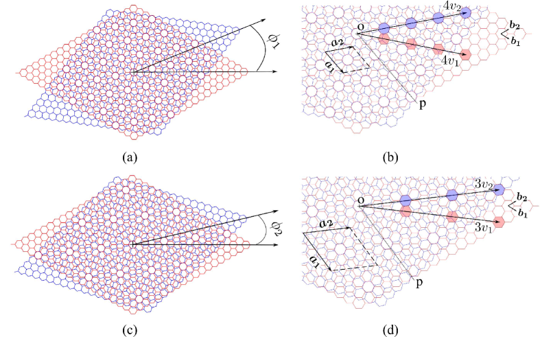
Figure 1: Schematic of periodic moiré lattices and unit cell. The rotation angle is $\phi_{1}=21.78^{\circ}$ in (a) and $\phi_{2}=13.17^{\circ}$ in (c). (b,d) Enlarged view of the lattices, along with lattice vectors. The blue and red shaded hexagons overlap when the two lattices coincide (at $\phi=0$). The moiré lattice in (a,b) has the smallest unit cell.

Figure 1 displays examples of hexagonal moiré lattices, along with their unit cells and lattice vectors. They are formed by stacking two identical hexagonal lattices with a relative rotation between them. The rotation is about the center of a hexagon with respect to its out-of-plane axis. The blue and red lattices are identical, but rotated relative to each other about $O$. The lattice vectors of the red hexagonal lattice are $\bm{b_{1}}$, $\bm{b_{2}}$ with $60^{\circ}$ angle between them, and the unit cell length is $b$. For an arbitrary relative rotation, the resulting pattern is not periodic. At specific rotation angles, a periodic pattern does result. These angles are hereby called moiré angles.

Let us discuss the conditions under which a periodic moiré lattice arises. We analyze the configuration that results when the blue lattice, which is initially coincident with the red one, is rotated about $O$. Two videos are presented in the supplementary materials on this rotation, illustrating the formation of the two distinct moiré lattices of Fig. 2(a,c). Let us fix this rotation center $O$ as the origin of our coordinate system. The key observation is that a periodic moiré lattice results when the center of a hexagon in a blue lattice coincides with the center of another hexagon in a red lattice away from the origin. The distance between the hexagon center and the rotation center $O$ should be identical for a pair of hexagons, one each from the blue and red lattice. Let us consider a hexagon in the red lattice with center $\bm{v}_{1}$ at

$$\bm{v_{1}}=m\bm{b_{1}}+n\bm{b_{2}},\;\;\;m,n\in\mathbb{Z},\;\;\;m>n,\;\;\;\gcd(m,n)=1.$$ (1)

Its distance from the center is $\|\bm{v_{1}}\|=b\sqrt{m^{2}+mn+n^{2}}$. It is the nearest red shaded hexagon from the center in the examples in Figs. 1(b,d). Due to the $C_{6}$ (6-fold rotation) symmetry of the hexagonal lattice, there are multiple hexagons in the blue lattice at the same distance. A simple choice for a hexagon in the blue lattice is $\bm{v_{2}}=n\bm{b_{1}}+m\bm{b_{2}}$, which satisfies $\|\bm{v_{1}}\|=\|\bm{v_{2}}\|$. The rotation angle (moiré angle) $\phi$ is thus the angle between $\bm{v_{1}}$ and $\bm{v_{2}}$, given by

$$\cos\phi=\dfrac{\bm{v_{1}.v_{2}}}{\|\bm{v}_{1}\|\|\bm{v}_{2}\|}=\dfrac{m^{2}/2+n^{2}/2+2mn}{m^{2}+n^{2}+mn}.$$ (2)

Let us see why the resulting bilayered (moiré) lattice is periodic along 2 directions and derive the lattice vectors of its unit cell. Note that any integer multiple of $\bm{v_{1}}$, i.e., $q\bm{v_{1}}$ is also the center of a hexagon in the red lattice. In addition, this hexagon goes to $q\bm{v_{2}}$ after rotation, as the angle between $q\bm{v_{1}}$ and $q\bm{v_{2}}$ is also $\phi$. Thus the lattice is periodic along $\bm{v_{2}}$, with periodicity $\|\bm{v_{2}}\|$. Since both the hexagonal lattices have $C_{6}$ (6-fold rotation) symmetry about $O$, the combined lattice also has $C_{6}$ symmetry about $O$. The moiré lattice is thus also periodic along directions at angle $\pi/3$ from $\bm{v_{2}}$. We take its lattice vectors to be $\bm{v}_{2}$ and a vector at angle $-\pi/3$ from $\bm{v}_{2}$. In terms of the hexagonal lattice vectors, the moiré lattice vectors $(\bm{a}_{1},\bm{a}_{2})$ may be expressed as

$$\bm{a}_{1}=n(\bm{b_{1}}-\bm{b_{2}})+m\bm{b_{1}}=(m+n)\bm{b_{1}}-n\bm{b_{2}},\quad\bm{a_{2}}=n\bm{b_{1}}+m\bm{b_{2}}.$$ (3)

Figure 1(a,c) displays the periodic moiré lattices for $(m,n)=(2,1)$ and $(3,2)$. Their corresponding unit cells and lattice vectors are indicated in Fig. 1(b,d). The relative angles between the blue and red lattices for these lattices are $\phi_{1}=21.78^{\circ}$ and $\phi_{2}=13.17^{\circ}$. The blue and red shaded hexagons coincide when there is no relative rotation between the two lattices. As the blue lattice is rotated, the blue shaded hexagons move to the locations illustrated in the figure, and they lie along $\bm{v_{2}}$. The lattice vector $\bm{a_{1}}$ lies along the line labeled $OP$. Note from these examples that the unit cell size of the resulting lattice is, in general, different for different $\phi$ values.

In this work, we investigate the behavior of the lattice with the smallest moiré unit cell, due to its potential ease of fabrication with macro-scale components. To determine this unit cell, let us calculate the unit cell area $A$ for a lattice with unit vectors given by Eqn. (3). It is given by

$$A=\|\bm{a_{1}}\times\bm{a_{2}}\|=\dfrac{\sqrt{3}b^{2}}{2}\left(m^{2}+mn+n^{2}\right)=\dfrac{\sqrt{3}b^{2}}{4}\left(m^{2}+n^{2}+(m+n)^{2}\right).$$ (4)

For $m$ and $n$ distinct non-zero integers, a direct calculation shows that $A=7\sqrt{3}b^{2}/2$ is the minimum area for $m=2$, $n=1$. The lattice vectors are thus

$$\bm{a_{1}}=3\bm{b_{1}}-\bm{b_{2}},\;\;\;\bm{a_{2}}=\bm{b_{1}}+2\bm{b_{1}}.$$ (5)

Let us discuss the key properties of this lattice. The parallelogram with lattice vectors labeled in Fig. 1b displays the chosen unit cell, with the center of the hexagon at its center. This choice ensures that a finite-sized hexagon-shaped lattice will have 6-fold rotation symmetry. This property will be used later in Sec. III.2 to predict localized modes at corners. This unit cell has 14 nodes of the hexagonal lattice in each layer. Indeed, note that the underlying hexagonal lattice has 2 nodes per unit cell and its area is $\sqrt{3}b^{2}/2$. Comparing with the moiré unit cell area, we see that the latter is 7 times larger and it thus has 14 nodes. In addition, there are two nodes in each unit cell where the red and blue lattices coincide. These nodes are indicated by green circles in the inset of Fig. 2a. Their locations within the unit cell, with respect to the lower $60^{\circ}$ in this inset, are given by

$$\bm{p_{1}}=\bm{b_{1}}+\dfrac{\bm{b_{1}}+\bm{b_{2}}}{3},\;\;\;\bm{p_{2}}=2\bm{b_{1}}+\dfrac{2}{3}\left(\bm{b_{1}}+\bm{b_{2}}\right).$$ (6)

By checking explicitly, we note that $\bm{p_{1}}$ and $\bm{p_{2}}$ lie at different sub-lattice sites of each hexagonal lattice. In particular, $\bm{p_{1}}$ lies at the $\alpha$ ($\beta$) site in the red (blue) lattice, while $\bm{p_{2}}$ lies in the $\beta$ ($\alpha$) site. Thus the $\alpha$ ($\beta$) site of the red (blue) lattice coincides with the $\beta$ ($\alpha$) site of the red lattice at $\bm{p_{1}}$ ($\bm{p_{2}}$) in each unit cell.

II.2 Plate configuration and governing equations

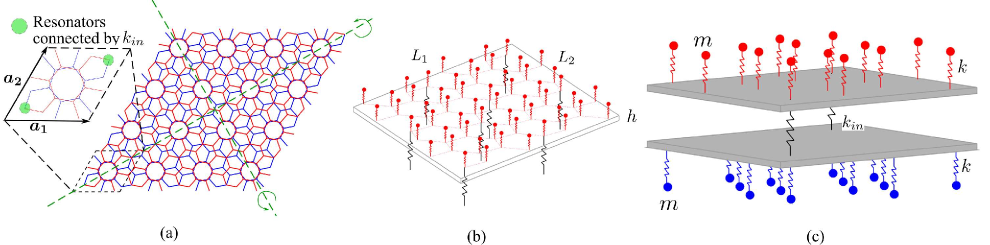
Figure 2: Schematic of bilayer elastic plate lattice. (a) Moiré lattice with a unit cell in the inset. Green circles indicate locations of coincident resonators in the two layers. Lattice has $C_{2}$ symmetry with respect to both its diagonals (green dash lines). (b) Top plate with resonators (red) in hexagonal lattice configuration. Black springs are at the coincident locations indicated in (a). (c) The moiré structure has two plates with resonators, and are coupled by the inter-layer springs, $k_{in}$.

We consider two thin infinite homogeneous and isotropic elastic plates supporting flexural (out-of-plane) vibrations. A set of identical discrete resonators with mass $m$ and stiffness $k$ are connected to each plate in a hexagonal lattice configuration. The resonators are located at the nodes of the hexagons. Let $\bm{r}_{\alpha\beta}$ indicate the position vectors of these resonators in each plate, with the index $\beta$ taking values in $\{t,b\}$ indicating the top and bottom plate, and $\alpha$ is an integer that labels the resonators in each plate. Figure 2b displays a schematic of the top plate with resonators. The bottom plate is rotated at an angle $\phi=21.78^{\circ}$ with respect to the center of a hexagon so that the resonator locations in the two plates resemble the moiré lattice as shown in Fig. 2a. Note that the edges of the hexagonal lattice in Figs. 2(a,b) do not have any physical meaning and are shown for clarity. The unit cell of the resulting lattice is indicated by dashed at the bottom left corner in Fig. 2a, along with its expanded view in the inset. Similar to the hexagonal lattice, the lattice vectors of the moiré lattice are also at $60^{\circ}$ to each other. As discussed above, it has 14 nodes in each layer with 2 nodal locations where the top and bottom layers coincide, as indicated by the green circles in the inset. The two plates are coupled by inter-layer springs of stiffness $k_{in}$ at these coinciding locations. Figure 2c displays a schematic of the fully assembled bilayered structure.

As noted earlier, each layer and thus the infinite lattice has $6$-fold rotation symmetry about an axis through the unit cell center. In addition, the lattice also has a 2-fold rotation symmetry about both the short and long in-plane diagonals, as indicated by the dashed lines in Fig. 2a. Indeed, when the lattice is rotated by $180^{\circ}$ about a diagonal, the top plate resonators go to the bottom plate resonators’ locations. The resulting structure is thus identical to that prior to rotation. Note that this operation is not equivalent to simply interchanging the top and bottom layers, as the latter will result in a different lattice.

Let us now present the governing equations for elastic waves in this bilayered structure. We assume that the out-of-plane modes are decoupled from the in-plane longitudinal and shear modes. In addition, we assume each resonator has one degree of freedom and can move out-of-plane. The out-of-plane displacement of a resonator located at $\bm{r}_{\alpha\beta}$ and the mid-plane section of plate $\beta$ are are denoted by $w_{\alpha\beta}$ and $w_{\beta}$, respectively. The dynamics of these thin plates are modeled using the Kirchhoff-Love theory. The equation of motion of the combined structure having $N$ moiré unit cells is given by [17, 43]

$$D\nabla^{4}w_{\beta}+\rho h\ddot{w}_{\beta} =-\sum_{\alpha=1}^{14N}k(w_{\beta}-w_{\alpha\beta})\delta(\bm{x}-\bm{r}_{\alpha\beta})-\sum_{\alpha=1}^{2N}k_{in}(w_{\beta}-w_{\beta^{\prime}})\delta(\bm{x}-\bm{r}_{\alpha\beta}),$$ (7a)

$$m\ddot{w}_{\alpha\beta} =-k(w_{\alpha\beta}-w_{\beta}(\bm{r}_{\alpha\beta})).$$ (7b)

Here $\bm{x}=(x,y)$, which denotes the position vector of a point in the plane of the plates, and the gradient operator $\nabla$ in Eqn. (7a) is with respect to $\bm{x}$. The first term on the right-hand side of Eqn. (7a) accounts for force due to the resonators, while the last term is for the interaction between the two plates. Subscript $(\beta,\beta^{\prime})$ in this last term takes values $\{t,b\}$ and $\{b,t\}$ for the top and bottom plates, respectively. The plate bending stiffness is $D=Eh^{3}/12(1-\nu^{2})$, with thickness $h$, Young’s modulus $E$, Poisson’s ratio $\nu$ and its density is $\rho$. For $N$ moiré unit cells, the number of resonators in each plate and the number of inter-layer springs are $14N$ and $2N$, respectively. The following dimension and properties are chosen for our numerical calculations: unit cell length $a=26.5$ mm, $m=10^{-3}$ kg, $k=10$ kN/m, $k_{in}=2$ kN/m, $h=0.1$ mm, $E=70$ GPa, $\nu=0.33$, $\rho=2700$ kg/${\mathrm{m}}^{3}$. The material properties correspond to aluminium as the plate material.

III Unit cell analysis

Having introduced the lattice description and presented the governing equations, we now do a dispersion analysis over its unit cell using the plane wave expansion method. We apply the approach followed in prior works on elastic plates with square and hexagonal array of resonators [44, 45, 17]. Then the topological properties of the dispersion bands are determined by computing the fractional corner mode $Q$, which is the elastic analogue of the fractional charge in electronic crystals [22]. This quantity is used to predict the existence of localized modes at the corners of a finite moiré lattice structure.

III.1 Dispersion analysis

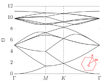
(a)

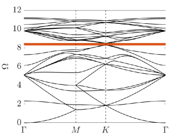
(b)

Figure 3: Dispersion diagram of the unit cell along the IBZ boundary (a) without inter-layer springs ($k_{in}=0$) and (b) with inter-layer springs ($k_{in}\neq 0$). The shaded band in (b) indicates a bandgap opening at the $K$-point.

We use Floquet-Bloch theory with the plane wave expansion method to determine waves propagating through the bilayered lattice. For a plane wave propagating with frequency $\omega$ and wave vector $\bm{\kappa}$, the displacement field in the plate may be expressed as

$$w_{\beta}(\bm{x},t)=e^{i(\omega t+\bm{\kappa}\cdot\bm{x})}W_{\beta}(\bm{x}).$$ (8)

where $W_{\beta}(\bm{x})$ is a periodic function with periodicity of the moiré unit cell. This periodic function can be expressed using a Fourier series as $\sum_{l_{1}}\sum_{l_{2}}W_{l_{1}l_{2}\beta}e^{i(l_{1}\bm{g_{1}}\cdot\bm{x}+l_{2}\bm{g_{2}}\cdot\bm{x})}$, with $\bm{g_{1},g_{2}}$ being the reciprocal lattice vectors of the moiré lattice. They satisfy $\bm{g_{i}}\cdot\bm{a_{j}}=2\pi\delta_{ij}$ and are given by $\bm{g_{1}}=2\pi(1/a,-1/\sqrt{3}a)$ and $\bm{g_{2}}=2\pi(0,2/\sqrt{3}a)$. The summation indices run over all integers, but for computation purposes, we truncate the summations at $T$ terms and use the approximation

$$w_{\beta}(\bm{x},t)=e^{i(\omega t+\bm{\kappa.x})}\sum_{\begin{subarray}{c}l_{1},l_{2}=-T\end{subarray}}^{T}e^{i(l_{1}\bm{g_{1}}+l_{2}\bm{g_{2}})\cdot\bm{x}}W_{l_{1}l_{2}\beta}.$$ (9)

Here, $W_{l_{1}l_{2}\beta}$ denotes the plane wave coefficient subscripted by integers $l_{1},l_{2}$ and finite number $(2T+1)^{2}$ of terms are considered. The resonator displacement can be expressed as

$$w_{\alpha\beta}(t)=e^{i(\omega t+\bm{\kappa}\cdot{\bm{r}_{\alpha\beta}})}W_{\overline{\alpha}\beta}.$$ (10)

Here the index $\overline{\alpha}$ takes values in $\{1,2,...,14\}$ and labels the resonators in a reference unit cell, while the index $\alpha$ is an integer that labels resonators in an arbitrary unit cell in the lattice.

Let us derive the discrete form of the governing equations over the unit cell. Substituting the plate and resonator displacements into Eqn. (7a), multiplying by $e^{-i\bm{(k+g^{\prime}).x}}$ and integrating over the unit cell gives an equation for each $W_{l_{1}l_{2}\beta}$. Similarly, substituting the displacements into Eqn. (7b) gives an equation for each $W_{\bar{\alpha}\beta}$. The detailed derivations are presented in Appendix A.1. The resulting discretized governing equations are

$$\omega^{2}W_{l^{\prime}_{1}l^{\prime}_{2}\beta} =\dfrac{D}{\rho Ah}{\lvert\bm{\kappa}+\bm{g^{\prime}}\rvert^{4}}W_{l^{\prime}_{1}l^{\prime}_{2}\beta}+\frac{k}{\rho Ah}\sum_{\begin{subarray}{c}\alpha=1\end{subarray}}^{14}e^{-i\bm{g^{\prime}}\cdot\bm{r}_{\alpha\beta}}\left(\sum_{\begin{subarray}{c}l_{1},l_{2}=-T\end{subarray}}^{T}e^{i\bm{g}\cdot\bm{r}_{\alpha\beta}}W_{l_{1}l_{2}\beta}-W_{\overline{\alpha}\beta}\right)$$

$$\qquad\qquad\qquad+\frac{k_{in}}{\rho Ah}\sum_{\begin{subarray}{c}\alpha=1\end{subarray}}^{2}e^{-i\bm{g^{\prime}}\cdot\bm{r}_{\alpha\beta}}\left(\sum_{\begin{subarray}{c}l_{1},l_{2}=-T\end{subarray}}^{T}e^{i\bm{g}\cdot\bm{r}_{\alpha\beta}}(W_{l_{1}l_{2}\beta}-W_{l_{1}l_{2}\beta^{\prime}})\right),$$ (11a)

$$\omega^{2}W_{\overline{\alpha}\beta} =-\frac{k}{m}\sum_{\begin{subarray}{c}l_{1},l_{2}=-T\end{subarray}}^{T}e^{i\bm{g}.\bm{r}_{\alpha\beta}}W_{l_{1}l_{2}\beta}+\frac{k}{m}W_{\overline{\alpha}\beta}.$$ (11b)

Here $\bm{g}=l_{1}\bm{g_{1}}+l_{2}\bm{g_{2}}$, $\bm{g^{\prime}}=l^{\prime}_{1}\bm{g_{1}}+l^{\prime}_{2}\bm{g_{2}}$ and $A=\sqrt{3}a^{2}/2$ is the unit cell area. Equations (11a) and (11b) together constitute an eigenvalue problem and its solution gives the dispersion relation of the unit cell yielding the frequencies $\omega$ at specific wave number, $\bm{\kappa}$. We present results for calculations with $T=10$. Increasing $T$ beyond this value did not result in a noticeable change in the results. Finally, the frequency $\omega$ is expressed in non-dimensional form using the normalization $\Omega=\sqrt{\rho a^{4}h/D}\omega$.

As discussed earlier in Sec. II.2, the infinite lattice has $6$-fold rotation symmetry about an out of plane axis through the unit cell center and 2-fold rotation symmetry about its in-plane diagonals. Thus its Brillouin zone is a hexagon and its irreducible Brillouin zone (IBZ) comprises of a triangle whose corners are the high symmetry points $\Gamma=(0,0)$, $M=(\pi,\pi/\sqrt{3})$ and $K=(2\pi/3,2\pi/\sqrt{3})$. Here, we examine the dispersion surfaces along the boundary of the IBZ.

Figure 3 displays the dispersion diagram of a unit cell for points along $\Gamma{\text{-}}M{\text{-}}K{\text{-}}\Gamma$ in the irreducible Brillouin zone (IBZ) for two cases: (a) the plates are uncoupled, $k_{in}=0$ and (b) coupled by inter-layer springs, $k_{in}\neq 0$. The inset in (a) has a schematic of the Brillouin zone, IBZ, along with the high symmetry points. Since the spectrum of $\nabla^{4}$ operator in Eqn. (7a) is unbounded, the exact solution has an infinite number of frequencies at each wave vector. There is a huge bandgap above the first 28 dispersion branches in both cases, and we restrict attention to these branches only. For the uncoupled plate case, the dispersion diagram in Fig. 3(a) has a Dirac cone at $K$ point, consistent with a Dirac cone that arises in a hexagonal lattice. A bandgap opens at that $K$ point when inter-layer springs are added, indicated by the shaded rectangle in Fig. 3(b). In addition, two branches become isolated from the remainder of the dispersion curves, consistent with other studies which find isolated flat bands at much smaller moiré angles [16].

III.2 Localized mode prediction by computing fractional corner mode $Q$

We use the dispersion analysis to determine if a finite moiré structure has localized modes at its boundary. The bulk edge correspondence principle relates the symmetry and topological properties of the Bloch modes in an infinite lattice to the modes localized on the boundaries of a finite lattice [21, 46]. The presence of localized modes can be predicted by computing appropriate topological invariants. Here, we will determine the elastic analog of the fractional corner charge $Q$, which has been introduced to predict and demonstrate localized modes in electronic and photonic media [21, 22, 47].

The fractional corner mode $Q$ is a topological invariant determining the existence of higher order topological mode in the bandgap. This quantity measures the change in rotational symmetry of the Bloch modes as we traverse the dispersion surface. It is expressed in terms of the number of specific rotational symmetry eigenvalues of the Bloch modes at the high symmetry points. All the dispersion branches below the bandgap are considered to compute $Q$. There are 14 bands below the band gap shown in Fig. 3(b) for the moiré lattice. Figure 4 displays the distribution of these $14$ frequencies at the various high symmetry points. We note that there are several degenerate sets of frequencies.

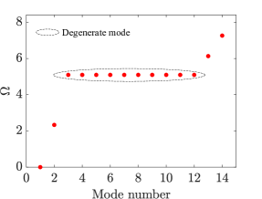
(a)

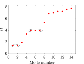
(b)

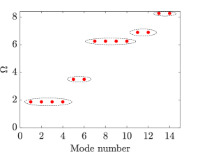
(c)

Figure 4: Frequencies of first $14$ bands below the bandgap at various high symmetry points of the irreducible Brillouin zone. There are a number of degenerate modes, which require a Gram Schmidt procedure to determine their rotational eigenvalue $\lambda_{p}$.

Before computing $Q$, let us discuss how a mode shape at the high symmetry points transforms as the lattice is rotated by an angle about the center of a unit cell. First, let us consider the high symmetry point $K$ and the rotation angle is $2\pi/3$. Under this rotation, the lattice geometry looks identical to that prior to rotation. Let $\bm{R}(\theta)$ the rotation matrix given by

$$\bm{R}(\theta)=\begin{pmatrix}\cos\theta&-\sin\theta\\ \sin\theta&\cos\theta\end{pmatrix},$$

and let $\bm{R}_{1}=\bm{R}(2\pi/3)$. Recall that the bilayered plate has 6-fold rotation symmetry about a unit cell center and thus remains identical when rotated by $\theta$. Let us indicate a plane wave with wave vector $\bm{\kappa}$ by $w_{\beta}(\bm{x},\bm{\kappa})$. It is also a function of $t$ and $\omega$, these are not indicated for brevity. Thus for every plane wave $w_{\beta}(\bm{x},\bm{\kappa})$, there is a corresponding plane wave with wave vector $\bm{R}\bm{\kappa}$, whose mode shape is $w_{\beta}(\bm{R}\bm{x},\bm{R}\bm{\kappa})$. This condition leads to the relation

$$w_{\beta}\left(\bm{x},\bm{\kappa}\right)=w_{\beta}\left(\bm{R}_{1}\bm{x},\bm{R}_{1}\bm{\kappa}\right)=w_{\beta}\left(\bm{R}_{1}\bm{x},\bm{\kappa}-\bm{g_{1}}-\bm{g_{2}}\right).$$ (12)

The second equality in the above equation follows by observing that the wave vector at $K$ satisfies $\bm{R}_{1}\bm{\kappa}=\bm{\kappa}-(\bm{g_{1}}+\bm{g_{2}})$, i.e., it translates by $-(\bm{g_{1}}+\bm{g_{2}})$ when rotated by $\theta=2\pi/3$. The Bloch mode shapes at wave vector $\bm{\kappa}-\bm{g_{1}}-\bm{g_{2}}$ are identical to that at $\bm{\kappa}$, as the term $e^{-i(\bm{g_{1}}+\bm{g_{2}})\cdot\bm{x}}$ relating them in Eqn. (8) is a periodic function [48]. Each set of corresponding Bloch modes at these two wave vectors may differ by a phase factor $\lambda$ as we continuously traverse the reciprocal lattice [49]. Hence, we have $w_{\beta}(\bm{x},\bm{\kappa}-\bm{g_{1}}-\bm{g_{2}})=\lambda w_{\beta}(\bm{x},\bm{\kappa})$. Substituting this relation for a point $\bm{R_{1}x}$ into the right side of Eqn. (12), we see that the displacements at $\bm{x}$ and $\bm{R}_{1}\bm{x}$ in a Bloch mode shape at the $K$ point are related by

$$w_{\beta}\left(\bm{x},\bm{\kappa}\right)=\lambda w_{\beta}(\bm{R}_{1}\bm{x},\bm{\kappa}).$$ (13)

Applying Eqn. (13) successively three times, we get the relation $w_{\beta}(\bm{x},\bm{\kappa})=\lambda^{3}w_{\beta}(\bm{R}_{1}^{3}\bm{x},\bm{\kappa})$. Noting that $\bm{R}_{1}^{3}$ is the identity matrix, we have $\lambda^{3}=1$. Its solutions are

$$\lambda_{p}=e^{i2\pi(p-1)/3},\;p\in\{1,2,3\}.$$

Thus each mode shape $w_{\beta}(\bm{x})$ at the high symmetry point $K$ satisfies Eqn. (13) for a specific value of $\lambda_{p}$. This $\lambda_{p}$ can thus be viewed as the eigenvalue of the rotational symmetry operator $\bm{R}_{1}$ for the mode shape.

Let us now describe the procedure to find the rotational eigenvalue $\lambda_{p}$ for each Bloch mode at the $K$ point. We project a mode shape into the subspace where a function $u(\bm{x})$ satisfies $u(\bm{R}_{1}\bm{x})=\lambda_{p}u(\bm{x})$. The projected mode is given by

$$w_{\beta}^{p}(\bm{x})=\dfrac{1}{3}\left(w_{\beta}(\bm{x})+\lambda_{p}^{-1}w_{\beta}(\bm{R_{1}x})+\lambda_{p}^{-2}w_{\beta}(\bm{R_{1}^{2}x})\right),\;p\in\{1,2,3\}.$$

By direct substitution, we can verify that any mode shape is decomposed into three parts $w_{\beta}^{p}$, that satisfy $w_{\beta}(\bm{x})=w_{\beta}^{1}(\bm{x})+w_{\beta}^{2}(\bm{x})+w_{\beta}^{3}(\bm{x})$. If a mode shape has rotational eigenvalue $\lambda_{q},q\in\{1,2,3\}$, then the component $w_{\beta}^{q}$ is non-zero, while the other two projected components are zero. For example, if a mode satisfies $w_{\beta}(\bm{x})=\lambda_{1}w_{\beta}(\bm{R_{1}}\bm{x})$, then $w_{\beta}^{1}(\bm{x})=w_{\beta}(\bm{x})$ and $w_{\beta}^{2}(\bm{x})=w_{\beta}^{3}(\bm{x})=0$. Thus examining the norms or magnitudes of $w_{\beta}^{p}(\bm{x})$ suffices to identify $\lambda_{p}$ for a non-degenerate mode. Next, let us discuss how to deal with a set of modes with degenerate frequencies. Here $w^{p}_{\beta}(\bm{x})$, determined by the above equation, can all be non-zero, as $w_{\beta}(\bm{x})$ may be a linear combination of mode shapes with distinct $\lambda_{p}$. To resolve this, we first determine $w_{\beta}^{p}(\bm{x})$ for all the mode shapes, say $n_{d}$, at a particular degenerate frequency. Then, for each $p$, a Gram-Schmidt procedure is done on the $n_{d}$ projected modes $w_{\beta}^{p}(\bm{x})$. The number of orthogonal modes with non-zero norm gives the number of independent $w_{\beta}^{p}(\bm{x})$, which is equal to the number of modes with rotational eigenvalue $\lambda_{p}$ in this set of $n_{d}$ modes.

We follow a similar approach to determine the rotational eigenvalues at the other high symmetry points $M$ and $\Gamma$. The wave vector at $M$ satisfies $\bm{R}(\pi)\bm{\kappa}=\bm{\kappa}-\bm{g_{1}}-\bm{g_{2}}$. Again, we note that the lattice looks identical prior to and after rotation by $\theta=\pi$. Using the same steps as for the $K$ point, the corresponding $\lambda_{p}$ are

$$\lambda_{p}=e^{i2\pi(p-1)/2}=(-1)^{p-1},\;p\in\{1,2\},$$

and the projected modes are

$$w_{\beta}^{p}(\bm{x})=\dfrac{1}{2}\left(w_{\beta}(\bm{x})+(-1)^{p-1}w_{\beta}(\bm{R}(\pi)\bm{x})\right),\;p\in\{1,2\}.$$

Examining the norms of $w^{p}_{\beta}$ or using a Gram Schmidt procedure for the sets with degenerate frequencies allows us to determine $\lambda_{p}$ for each mode. The wave vector at $\Gamma$ point satisfies both $\bm{R}(2\pi/3)\bm{\kappa}=\bm{\kappa}$ and $\bm{R}(\pi)\bm{\kappa}=\bm{\kappa}$. For each mode at $\Gamma$, we can thus determine the rotational eigenvalues $\lambda_{p}$ for rotations by $2\pi/3$ and $\pi$. The mode shapes $w^{p}_{\beta}$ corresponding to each $\lambda_{p}$ for all the high symmetry points are presented in Appendix B, see Figs. 9- 12.

The fractional corner mode $Q$, analogous to its electronic counterpart, is given by [42]

$$Q=\dfrac{[M_{1}^{(2)}]}{4}+\dfrac{[K_{1}^{(3)}]}{6}\mod 1.$$ (14)

Here, $[M_{1}^{(2)}]$ is the difference between the number of modes at $M$ and $\Gamma$ points that have $\lambda_{p}=1$ under rotation by $\theta=\pi$. Similarly, $[K_{1}^{(3)}]$ denotes the difference between the number of mode shapes at $K$ and $\Gamma$ points with $\lambda_{p}=1$ under rotation by $\theta=2\pi/3$. Counting the number of mode shapes with $p=1$ at the high symmetry points below the bandgap, we have from Eqn. (14)

$$Q=\dfrac{(6-8)}{4}+\dfrac{(4-6)}{6}=\dfrac{-5}{6}=\dfrac{1}{6}\mod 1.$$ (15)

A non-zero value of $Q$ in Eqn. (15) confirms the non-trivial topological nature of the bandgap, which in turn, implies the existence of corner localized modes in a finite structure.

We apply the framework established by Hughes and coworkers [22] in the context of electronic waves and charges to predict the location of localized modes. This framework allows us to express the stiffness matrix of any $C_{6}$ symmetric structure as a direct sum of copies of the stiffness matrices of primitive generator lattices. The topological invariants, like $Q$, are a sum of the corresponding $Q$ values of these primitive generators. We consider two primitive generators: $h_{4b}$, $h_{3c}$ that have nontrivial topological properties. Here, a lattice with notation $h_{mW}$ has $m$ bands below the bandgap and a Wannier center at location $W$ [22]. The lattice schematics, unit cell and dispersion diagrams for these two lattices are presented in Appendix C.

We computed the fractional corner modes for these primitive generator lattices by considering both 6-fold and 3-fold rotation symmetry. The values are $Q_{6}=2/3,\;Q_{3}=1/3$ for the $h4b$ lattice and $Q_{6}=1/2,\;Q_{3}=0$ for the $h3c$ lattice. Here, the subscripts of $Q$ indicate the rotation symmetry of the finite structure. Thus $Q_{6}$ and $Q_{3}$ determine localized modes at $120^{\circ}$ and $60^{\circ}$ corners, respectively. These values show that the $h4b$ lattice has a localized mode at $60^{\circ}$ corner, while both lattices have at $120^{\circ}$ corner. Noting that $Q$ of the moiré lattice may be expressed as $Q=1/6=2/3+1/2\;(\mod 1)$, we infer that the moiré lattice is equivalent to stacking a copy of each of these these two primitive generators, along with copies of a lattice ($t$) that has trivial topological properties. In other words, the stiffness matrix of the moiré lattice, expressed in the basis of the first 28 dispersion bands, is equivalent to the direct sum $h4b\oplus h3c\oplus 7t$. This direct sum, along with the $Q$ values of the primitive generators, indicates the existence of corner localized modes at both $120^{\circ}$ and $60^{\circ}$ corners in our moiré structure. Indeed, the latter case of $60^{\circ}$ corner localized mode is inferred by noting that the $Q_{3}$ value of our moiré lattice is $1/3+0=1/3$.

IV Numerical results of finite plate

In this section, the predictions of corner localized modes in Sec. III.2 are verified by determining the mode shapes and frequency response under external excitation on a finite plate. We show that these localized modes are excited even when an external force is applied far from the corner.

IV.1 Bulk and localized mode shapes

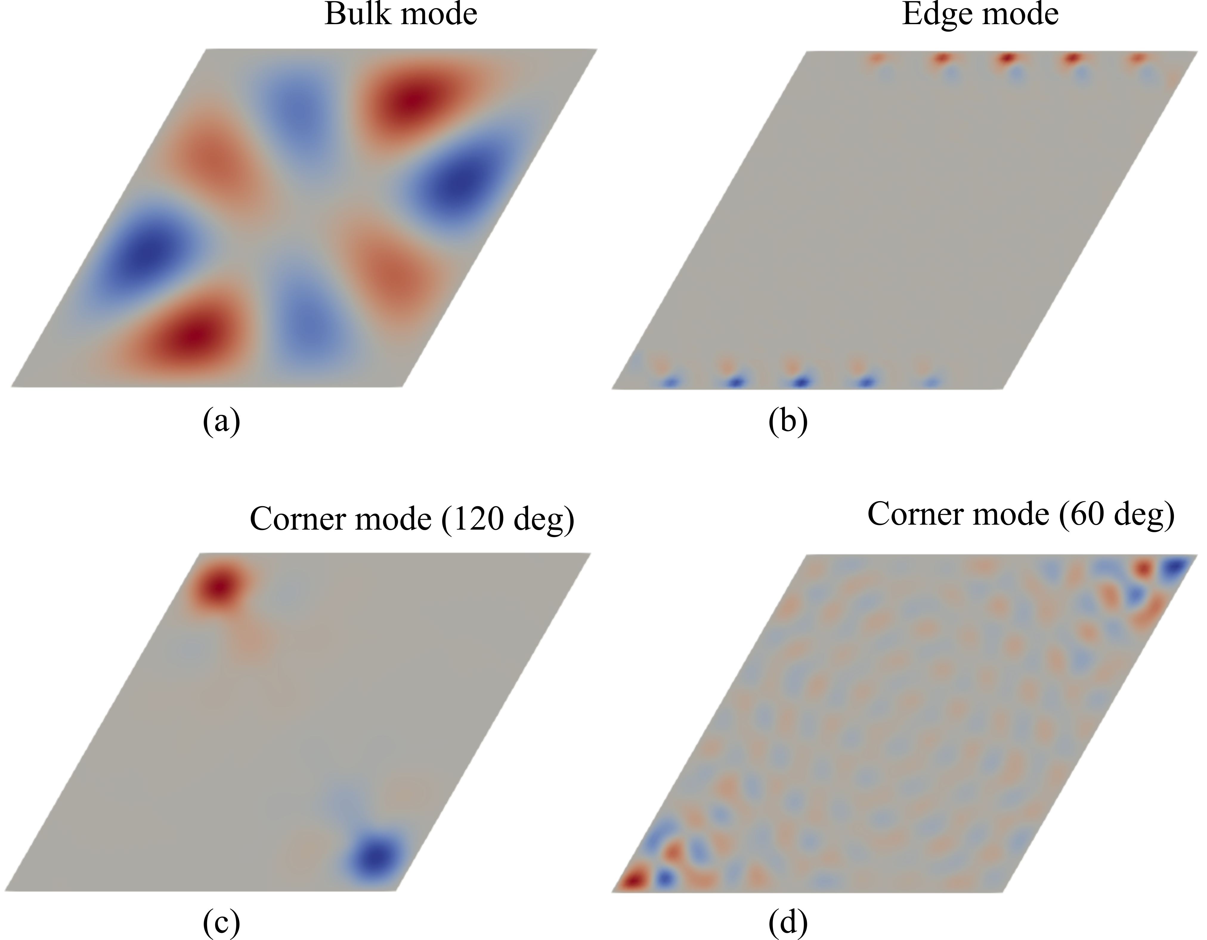
Figure 5: Mode shapes of a finite plate with simply-supported boundary conditions. Displacement contours of top plate for (a) a typical bulk mode ($\Omega=0.70$), (b) an edge mode ($\Omega=13.71$), corner modes at (c) $120^{\circ}$ corner ($\Omega=2.34$) and (d) $60^{\circ}$ corner ($\Omega=8.19$).

We consider a finite plate of $n_{1}\times n_{2}=6\times 6$ moiré unit cells along $\bm{a_{1}}$, $\bm{a_{2}}$ directions. The sides of the plate are of lengths $L_{1}$ and $L_{2}$, both equal to $6a$. The four sides of the plate are simply supported, implying zero displacement and zero bending moment about an axis along the boundary. At each boundary point, these conditions may be expressed as [50]

$$w_{\beta}=0,\quad M_{\eta}=\dfrac{\partial^{2}w_{\beta}}{\partial\eta^{2}}+\nu\dfrac{\partial^{2}w_{\beta}}{\partial\tau^{2}}=0,$$

with $\eta$ and $\tau$ being coordinates normal to and along the boundary.

We introduce and work with a coordinate system whose axes $(x_{1},x_{2})$ are aligned with the lattice vectors of the moiré lattice. The boundary conditions and solution basis functions are conveniently expressed in this coordinate system. To determine the governing equations in this coordinate system, let us determine its relation with the Cartesian coordinate system having axes $(x,y)$. Let us consider an arbitrary point with position vector $\bm{x}$ in the two coordinate systems. It is given by $\bm{x}$ = $x\bm{e_{x}}$ + $y\bm{e_{y}}=x_{1}\bm{e_{1}}$ + $x_{2}\bm{e_{2}}$, with $(\bm{e_{x}},\bm{e_{y}})$ and $(\bm{e_{1}},\bm{e_{2}})$ being unit vectors in the two coordinate systems. Taking dot products with $\bm{e_{x}}$ and $\bm{e_{y}}$ gives the relations $x=x_{1}+x_{2}/2$ and $y=\sqrt{3}x_{2}/2$. They can be inverted to get $x_{1}=x-y/\sqrt{3}$ and $x_{2}=2y/\sqrt{3}$.

The boundary conditions in the new coordinate system become

$$w_{\beta}(x_{1}=0,x_{2})=w_{\beta}(x_{1}=L_{1},x_{2})=w_{\beta}(x_{1},x_{2}=0)=w_{\beta}(x_{1},x_{2}=L_{2})=0,$$

$$\partialderivative[2]{w_{\beta}}{x_{1}}\bigg{|}_{(x_{1}=0)}=\partialderivative[2]{w_{\beta}}{x_{1}}\bigg{|}_{(x_{1}=L_{1})}=\partialderivative[2]{w_{\beta}}{x_{2}}\bigg{|}_{(x_{2}=0)}=\partialderivative[2]{w_{\beta}}{x_{2}}\bigg{|}_{(x_{2}=L_{2})}=0.$$

The plate displacement, $w_{\beta}(\bm{x},t)$ is approximated using a set of harmonic basis functions as

$$w_{\beta}(\bm{x},t)=e^{i\omega t}\sum_{\begin{subarray}{c}p=1\end{subarray}}^{N_{1}}\sum_{\begin{subarray}{c}q=1\end{subarray}}^{N_{2}}\sin{\frac{p\pi x_{1}}{L_{1}}\sin{\frac{q\pi x_{2}}{L_{2}}}}W_{pq\beta}.$$ (16)

Note that these basis functions satisfy all the above boundary conditions. Similarly, the resonator displacements, $w_{\alpha\beta}(t)$ can be written as

$$w_{\alpha\beta}(t)=e^{i\omega t}W_{\alpha\beta},$$ (17)

with the index $\alpha$ ranging from $1$ to $14\times n_{1}\times n_{2}$.

Let us now derive the discrete approximations of the governing equations for vibration at frequency $\omega$. Substituting the above displacements into Eqn. (7a), multiplying by $\sin(p^{\prime}\pi x_{1}/L_{1})\sin(q^{\prime}\pi x_{2}/L_{2})$ and integrating over the finite plate leads to an equation for each basis function. Similarly, substituting the displacements into Eqn. (7b) gives an equation for each resonator displacement amplitude $W_{{\alpha}\beta}$. The detailed derivations are presented in Appendix A.2. The discretized governing equations thus obtained are

$$\omega^{2}W_{p^{\prime}q^{\prime}\beta} =\frac{16\pi^{4}D}{9\rho hL_{1}^{4}L_{2}^{4}}\left(p^{\prime 4}L_{2}^{4}+3p^{\prime 2}q^{\prime 2}L_{1}^{2}L_{2}^{2}+q^{\prime 4}L_{1}^{4}\right)W_{p^{\prime}q^{\prime}\beta}$$

$$\quad+\frac{32p^{\prime}q^{\prime}D}{9\rho h}\sum_{\begin{subarray}{c}p=1\\ p\neq p^{\prime}\end{subarray}}^{N_{1}}\sum_{\begin{subarray}{c}q=1\\ q\neq q^{\prime}\end{subarray}}^{N_{2}}\frac{pq}{L_{1}L_{2}}\left\{(\frac{p\pi}{L_{1}})^{2}+(\frac{q\pi}{L_{2}})^{2}\right\}\left[\frac{(-1)^{p+p^{\prime}}-1}{p^{2}-p^{\prime 2}}\right]\left[\frac{(-1)^{q+q^{\prime}}-1}{q^{2}-q^{\prime 2}}\right]W_{pq\beta}$$

$$\quad+\frac{8k}{\sqrt{3}\rho hL_{1}L_{2}}\sum_{\alpha=1}^{14n_{1}n_{2}}\sin{\frac{p^{\prime}\pi r_{\alpha\beta 1}}{L_{1}}\sin{\frac{q^{\prime}\pi r_{\alpha\beta 2}}{L_{2}}}}\left[\sum_{p=1}^{N_{1}}\sum_{q=1}^{N_{2}}\sin{\frac{p\pi r_{\alpha\beta 1}}{L_{1}}\sin{\frac{q\pi r_{\alpha\beta 2}}{L_{2}}}}W_{pq\beta}-W_{\alpha\beta}\right]$$

$$\quad+\frac{8k_{in}}{\sqrt{3}\rho hL_{1}L_{2}}\sum_{\alpha=1}^{2n_{1}n_{2}}\sin{\frac{p^{\prime}\pi r_{\alpha 1}}{L_{1}}\sin{\frac{q^{\prime}\pi r_{\alpha 2}}{L_{2}}}}\left[\sum_{p=1}^{N_{1}}\sum_{q=1}^{N_{2}}\sin{\frac{p\pi r_{\alpha 1}}{L_{1}}\sin{\frac{q\pi r_{\alpha 2}}{L_{2}}}}(W_{pq\beta}-W_{pq\beta^{\prime}})\right],$$ (18a)

$$\omega^{2}W_{\alpha\beta} =\dfrac{k}{m}W_{\alpha\beta}-\dfrac{k}{m}\sum_{p=1}^{N_{1}}\sum_{q=1}^{N_{2}}\sin{\frac{p\pi r_{\alpha\beta 1}}{L_{1}}\sin{\frac{q\pi r_{\alpha\beta 2}}{L_{2}}}}W_{pq\beta}.$$ (18b)

Here $\bm{r}_{\alpha\beta}=r_{\alpha\beta 1}\bm{e}_{1}+r_{\alpha\beta 2}\bm{e}_{2}$ and $\bm{r}_{\alpha}=r_{\alpha 1}\bm{e}_{1}+r_{\alpha 2}\bm{e}_{2}$ are the position vectors of resonators and inter-layer springs expressed in the $(x_{1},x_{2})$ coordinate system. Here, Eqn. (18a) and Eqn. (18b) together constitute an eigenvalue problem of the form $\omega^{2}\bm{v}=\bm{Kv}$, with $\bm{v}=[\bm{W_{pqt}};\bm{W_{pqb}};\bm{W_{\alpha t}};\bm{W_{\alpha b}}]$ being the vector whose components are coefficients of basis functions for both the plate and resonator displacements. $\bm{K}$ is the stiffness matrix containing the right-hand side terms in Eqn. (18a) and Eqn. (18b). The solution of the eigenvalue problem provides the mode shapes at the corresponding frequencies, $\omega$. Each mode shape has 4 parts: displacement fields of the top and bottom plates $w_{\beta}$, and the vector of resonator displacements $W_{\alpha\beta}$ in each plate.

Let us remark on the relation between the displacement fields in the plates based on symmetry considerations. Note that the finite bilayer structure also has $C_{2}$ symmetry about each of its diagonals, similar to the infinite lattice (see Fig. 2a). The mode shapes of the finite plate are thus eigenvectors of this symmetry operator. Since the $C_{2}$ rotation operator has eigenvalues $\lambda=\pm 1$, each mode shape remains the same or changes sign under a rotation by $\pi$ along a diagonal. We observe that this symmetry operation is equivalent to reflecting each plate in its plane about a diagonal, followed by interchanging the two plates. Thus, an equivalent way to express the above symmetry condition is the following: for each mode shape, if the top plate displacement field is reflected about a diagonal, it will be same $(\lambda=+1)$ or negative $(\lambda=-1)$ of the bottom plate displacement field. Note that the $\lambda$ values can be distinct when reflected about the short and long diagonals for a mode shape.

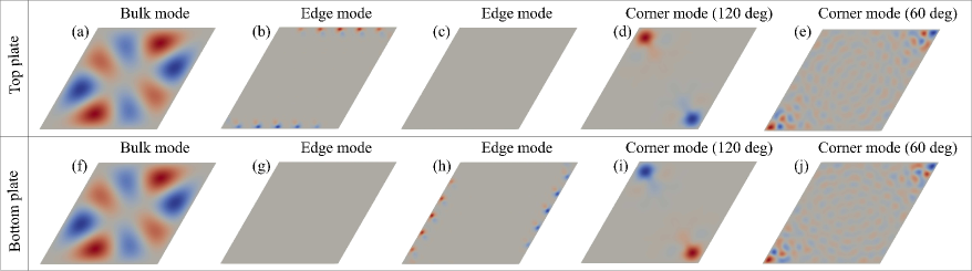
Figure 14: Displacement contours of top and bottom plate for (a, f) a typical bulk mode ($\Omega=0.70$), (b, c, g, h) an edge mode ($\Omega=13.71$), (d, i) corner mode at $120^{\circ}$ corner ($\Omega=2.34$) and (e, j) $60^{\circ}$ corner ($\Omega=8.19$). Top and bottom rows correspond to the top and bottom plate displacement contours, respectively.

The results are reported for calculations with $N_{1}=N_{2}=50$ terms. We also did calculations with $N_{1}=N_{2}=60$, and did not observe a noticeable difference in the mode shapes. Displacement contours at the top plate are illustrated in Fig. 5 for a few representative mode shapes. The bottom plate displacement field, top and bottom resonator displacements for these mode shapes are presented in Appendix D, see Figs. 14 and 15. We find that the resonator displacements are in phase with their plate displacements for all of these modes. As discussed above, a mode shape may change sign or remain unchanged under rotation by $\pi$ about a diagonal. This relation may be determined by examining the displacement fields of top and bottom plates. They are tabulated below for each mode in Fig. 5 and for each diagonal rotation axis. The modes that remain identical and that change sign under rotation are labeled even and odd, respectively.

-	Bulk	Edge	Corner($120^{\circ}$)	Corner($60^{\circ}$)
Short diagonal	odd	even	odd	odd
Long diagonal	odd	odd	even	even

Table 1: Symmetry property of the modes in Fig. 5 under $180^{\circ}$ rotation about its short and long diagonals.

The edge localized mode in Fig. 5b has a counterpart at the same frequency, that is localized at the other edges. The mode shape of this counterpart is included in Appendix D. These edge modes lie in the bandgap above the first 28 dispersion branches. They do not have a topological origin and may become bulk modes when boundary conditions or material properties are varied. In contrast, the corner localized modes shown in Fig. 5(c-d) arise due to the symmetry and topological properties of dispersion bands. The mode localized at the $120^{\circ}$ lies in the bulk band frequency, while the $60^{\circ}$ corner localized mode lies in the bandgap. These localized modes verify the prediction of higher order topological mode at both corners as discussed in Sec. III.2.

IV.2 Frequency response under harmonic excitation

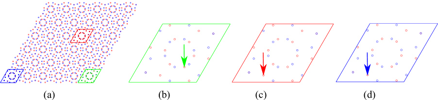
Figure 6: Schematic of the finite lattice showing different excitation and response locations. (a) Responses are evaluated over the unit cell indicated by parallelogram at $120^{\circ}$ corner, interior and $60^{\circ}$ corner. Excitations are given at a resonator in the top plate indicated by arrow in (b) $120^{\circ}$ corner, (c) interior and (d) $60^{\circ}$ corner.

Finally, let us analyze the effect of these topological corner localized modes on the steady-state dynamic response under external excitation. To this end, we determine the frequency response by applying a harmonic force and measuring the steady state response at various locations (see Fig. 6) in the finite lattice. An excitation $fe^{i\omega t}$ is applied at one resonator in the top plate, indicated by an arrow in Figs. 6(b-d). The equations for solving the frequency response is $\omega^{2}\bm{v}-\bm{Kv}=\bm{f}$, where $\bm{f}$ is the external force vector. It takes $1$ associated to the excitation point and rest values are $0$. The considered frequency spacing in the calculation is $\Delta\omega=1.0\times 10^{-2}$ rad/s, or in non-dimensional units, $\Delta\Omega=$4.50\text{\times}{10}^{-5}$$. For each case, responses are also observed at the $120^{\circ}$ corner, interior and $60^{\circ}$ corner region over a unit cell indicated by parallelogram in Fig. 6a. The response is computed using the expression

$$\frac{|u|}{f}=\sqrt{\sum_{\beta=\{t,b\}}\sum_{\alpha=1}^{14}\left|w_{\alpha\beta}\right|^{2}}.$$ (19)

To illustrate the effect of corner localized modes in Fig. 5(c-d) on the frequency response function of a finite plate, we excite it in a range of frequencies around these natural frequencies. Recall that the $120^{\circ}$ and $60^{\circ}$ corner localized mode frequencies are 2.34 and 8.19, respectively. At each frequency, we excite the lattice at 3 locations: at a $60^{\circ}$ and a $120^{\circ}$ corner, and in the interior, and determine the response of the unit cells at these locations using Eqn. (19). These locations are indicated in Fig. 6.

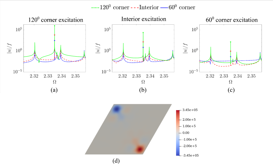
Figure 7: frequency response and displacement contour near the $120^{\circ}$ corner localized frequency. Excitation is given at (a) $120^{\circ}$ corner, (b) interior and (c) $60^{\circ}$ corner and response are also shown at $120^{\circ}$ corner, interior and $60^{\circ}$ corner. (d) Top plate displacement contour for $120^{\circ}$ corner excitation at frequency 2.34.

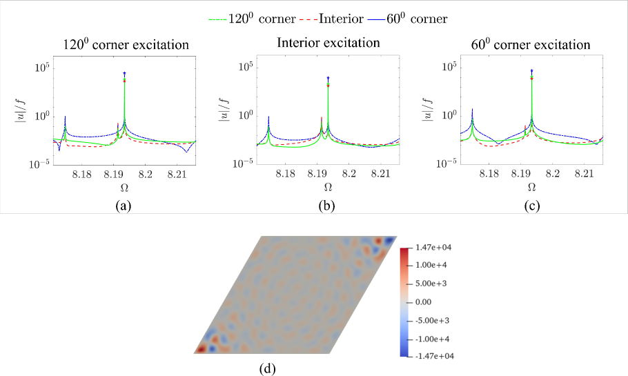
Figure 8: frequency response and displacement contour near the $60^{\circ}$ corner localized frequency. Excitation is given at (a) $120^{\circ}$ corner, (b) interior and (c) $60^{\circ}$ corner and response are also shown at $120^{\circ}$ corner, interior and $60^{\circ}$ corner. (d) Top plate displacement contour for $60^{\circ}$ corner excitation at frequency 8.19.

Figure 7(a-c) displays the frequency response near $\Omega=2.34$, with each sub-figure for a different excitation location. For the $120^{\circ}$ corner excitation, Fig. 7a displays the response at various locations in the finite plate indicated in Fig. 6a. The peak responses at all locations happen at frequency 2.34, as indicated by a “star” in the figure. The response of the $120^{\circ}$ corner unit cell is higher than at other locations, since it is close to the excitation point. Similarly, Fig. 7(b-c) displays the response for excitations at the interior and $60^{\circ}$ corner locations. Even when the excitation is far from the $120^{\circ}$ corner, the peak response at the localized mode frequency is the highest at this corner. This peak response shows that the corner localized mode gets excited regardless of the excitation location in the plate. In contrast, away from the localized mode frequency, we note that the response is higher close to the excitation location. See for example, the response to $60^{\circ}$ corner excitation in Fig. 7c. Figure 7d displays the displacement contours of the top plate for an excitation $\Omega=2.34$ at $120^{\circ}$ corner, which is similar to the mode shape in Fig. 5c. The displacement contours for excitation at interior and $60^{\circ}$ corner locations have similar profile, but with lower peak magnitudes of ${7.96}\times 10^{3}$ and ${4.95}\times 10^{1}$, respectively.

Similarly, Fig. 8(a-c) displays the frequency response around $\Omega=8.19$ for various excitation locations. Again, the peak response happens at the localized mode frequency and the $60^{\circ}$ corner has the highest displacement magnitude $|u|/f$, regardless of the excitation location. Figure 8d illustrates the displacement contour of top plate for excitation at $60^{\circ}$ corner, confirming that the steady-state response is localized at the $60^{\circ}$ corner. The displacement contours for excitation at the $120^{\circ}$ corner and interior have a similar profile, but with different maximum magnitudes of ${9.87}\times 10^{3}$ and ${2.66}\times 10^{3}$, respectively. These calculations verify the presence of corner localized modes at both corners of the finite moiré plates.

V Conclusions

We investigated corner localized modes that arise due to higher order topology in moiré lattices of bilayer elastic plates. Each plate has a hexagonal array of resonators and one of the plates is rotated an angle ($21.78^{\circ}$) which results in a periodic moiré lattice with the smallest area. The resulting structure opens a band gap when inter-layer springs are added. The fractional corner mode $Q$ is found to be $1/6$ for dispersion bands below the bandgap. The non-zero value of $Q$ indicates the non-trivial topological nature of the bandgap and predicts the existence of localized modes at all corners in the finite structure. Modal analysis on a finite plate showed the existence of these corner localized modes at both $60^{\circ}$ and $120^{\circ}$ corners. The first one lies in the bulk band frequency and the later one lies in the bandgap frequency. Finally, the frequency response under external excitation at various locations shows mode localization at these frequencies, consistent with the theoretical predictions. The considered continuous elastic moiré lattice structures open opportunities for seeking novel wave phenomena with potential applications in tunable energy localization, vibration isolation, and energy harvesting.

Appendix A Derivation of discrete governing equations

The detailed derivation of the discrete form of the governing equations in terms of the Fourier coefficients $W_{l_{1}l_{2}\beta}$ are presented for dispersion analysis and $W_{pq\beta}$ for finite plate analysis.

A.1 Dispersion analysis

We start by substituting the displacements in Eqns. (9) and (10) into the governing equation for the plate (7a), which leads to

$$(D{\lvert\bm{\kappa}+\bm{g}\rvert^{4}}-\rho h\omega^{2})\sum_{\begin{subarray}{c}l_{1},l_{2}=-T\end{subarray}}^{T}e^{i\bm{(k+g).x}}W_{l_{1}l_{2}\beta}=-k\sum_{\alpha=1}^{14N}\left[\sum_{\begin{subarray}{c}l_{1},l_{2}=-T\end{subarray}}^{T}e^{i\bm{(k+g).x}}W_{l_{1}l_{2}\beta}-e^{i\bm{\kappa.{\bm{r}_{\alpha\beta}}}}W_{\overline{\alpha}\beta}\right]\delta(\bm{x}-\bm{r}_{\alpha\beta})\\ -k_{in}\sum_{\alpha=1}^{2N}\left[\sum_{\begin{subarray}{c}l_{1},l_{2}=-T\end{subarray}}^{T}e^{i\bm{(k+g).x}}(W_{l_{1}l_{2}\beta}-W_{l_{1}l_{2}\beta^{\prime}})\right]\delta(\bm{x}-\bm{r}_{\alpha\beta}).$$ (20)

We work in the $(x_{1},x_{2})$ coordinate system, whose unit vectors are aligned with the moiré lattice vectors $(\bm{a_{1}},\bm{a_{2}})$. It is related to the Cartesian coordinate system by $x_{1}=x-y/\sqrt{3}$ and $x_{2}=2y/\sqrt{3}$. Multiplying by $e^{-i\bm{(k+g^{\prime}).x}}$, rearranging and integrating over a unit cell $\mathcal{D}$ gives

$$\int_{\mathcal{D}}\sum_{\begin{subarray}{c}l_{1},l_{2}=-T\end{subarray}}^{T}(D{\lvert\bm{\kappa}+\bm{g}\rvert^{4}}-\rho h\omega^{2})e^{i\bm{(g-g^{\prime}).x}}W_{l_{1}l_{2}\beta}dx_{1}\wedge dx_{2}\\ =-k\int_{\mathcal{D}}\sum_{\alpha=1}^{14N}\left[e^{-i\bm{g^{\prime}.x}}\left\{\sum_{\begin{subarray}{c}l_{1},l_{2}=-T\end{subarray}}^{T}e^{i\bm{g.x}}W_{l_{1}l_{2}\beta}-e^{i\bm{\kappa.({r}_{\alpha\beta}-x)}}W_{\overline{\alpha}\beta}\right\}\right]\delta(\bm{x}-\bm{r}_{\alpha\beta})dx_{1}\wedge dx_{2}\\ -k_{in}\int_{\mathcal{D}}\sum_{\alpha=1}^{2N}\left[e^{-i\bm{g^{\prime}.x}}\left\{\sum_{\begin{subarray}{c}l_{1},l_{2}=-T\end{subarray}}^{T}e^{i\bm{g.x}}(W_{l_{1}l_{2}\beta}-W_{l_{1}l_{2}\beta^{\prime}})\right\}\right]\delta(\bm{x}-\bm{r}_{\alpha\beta})dx_{1}\wedge dx_{2}.$$ (21)

Note that $dx_{1}\wedge dx_{2}=(\sqrt{3}/2)dx_{1}dx_{2}$ is the area of an infinitesimal parallelogram in $\mathcal{D}$. Using orthogonality of the functions $e^{i\bm{g}\cdot\bm{x}}$, we get

$$(D{\lvert\bm{\kappa}+\bm{g^{\prime}}\rvert^{4}}-\rho h\omega^{2})AW_{l_{1}^{\prime}l_{2}^{\prime}\beta}=-k\sum_{\alpha=1}^{14N}\left[e^{-i\bm{g^{\prime}.\bm{r}_{\alpha\beta}}}\left\{\sum_{\begin{subarray}{c}l_{1},l_{2}=-T\end{subarray}}^{T}e^{i\bm{g.\bm{r}_{\alpha\beta}}}W_{l_{1}l_{2}\beta}-W_{\overline{\alpha}\beta}\right\}\right]\\ -k_{in}\sum_{\alpha=1}^{2N}\left[e^{-i\bm{g^{\prime}.\bm{r}_{\alpha\beta}}}\left\{\sum_{\begin{subarray}{c}l_{1},l_{2}=-T\end{subarray}}^{T}e^{i\bm{g.\bm{r}_{\alpha\beta}}}(W_{l_{1}l_{2}\beta}-W_{l_{1}l_{2}\beta^{\prime}})\right\}\right].$$ (22)

Here $A=\sqrt{3}a^{2}/2$ is the area of the moire unit cell. Dividing both sides of the above equation by $\rho Ah$ and rearranging gives Eqn. (11a).

For the resonator, substituting the displacements in Eqns. (9) and (10) into their governing equations (7b) gives

$$-m\omega^{2}e^{i{\bm{\kappa.r_{\alpha\beta}}}}W_{\overline{\alpha}\beta}=-ke^{i{\bm{\kappa.r_{\alpha\beta}}}}W_{\overline{\alpha}\beta}+k\sum_{\begin{subarray}{c}l_{1},l_{2}=-T\end{subarray}}^{T}e^{i\bm{(k+g)}.\bm{r_{\alpha\beta}}}W_{l_{1}l_{2}\beta}.$$ (23)

Multiplying by $-e^{-i{\bm{\kappa.r_{\alpha\beta}}}}/m$ gives Eqn. (11b).

A.2 Derivation for finite plate frequencies and mode shapes

Let us derive the discrete equations that are used to determine the mode shapes and frequency response of a finite plate. Substituting the assumed displacement fields in Eqns. (16) and (17) into the governing equation Eqn. (7a) for a plate gives

$$\sum_{\begin{subarray}{c}p=1\end{subarray}}^{N_{1}}\sum_{\begin{subarray}{c}q=1\end{subarray}}^{N_{2}}\left[{\frac{1}{\sin^{4}{\theta}}}(\frac{p\pi}{L_{1}})^{4}+{\frac{6}{\sin^{2}{\theta}\tan^{2}{\theta}}}(\frac{p\pi}{L_{1}})^{2}(\frac{q\pi}{L_{2}})^{2}+\frac{1}{\sin^{4}{\theta}}(\frac{q\pi}{L_{2}})^{4}+{\frac{2}{\sin^{2}{\theta}}}(\frac{p\pi}{L_{1}})^{2}(\frac{q\pi}{L_{2}})^{2}-\frac{\rho h\omega^{2}}{D}\right]\cdot\\ W_{pq\beta}\sin{\frac{p\pi x_{1}}{L_{1}}\sin{\frac{q\pi x_{2}}{L_{2}}}}+\frac{4}{\tan{\theta}\sin^{3}{\theta}}\sum_{\begin{subarray}{c}p=1\end{subarray}}^{N_{1}}\sum_{\begin{subarray}{c}q=1\end{subarray}}^{N_{2}}\frac{p\pi}{L_{1}}\frac{q\pi}{L_{2}}\left\{(\frac{p\pi}{L1})^{2}+(\frac{q\pi}{L2})^{2}\right\}W_{pq\beta}\cos{\frac{p\pi x_{1}}{L_{1}}\cos{\frac{q\pi x_{2}}{L_{2}}}}\\ =-\frac{k}{D}\sum_{\alpha=1}^{14N}\left[\sum_{\begin{subarray}{c}p=1\end{subarray}}^{N_{1}}\sum_{\begin{subarray}{c}q=1\end{subarray}}^{N_{2}}W_{pq\beta}\sin{\frac{p\pi x_{1}}{L_{1}}\sin{\frac{q\pi x_{2}}{L_{2}}}}-W_{\alpha\beta}\right]\delta(\bm{x}-\bm{r}_{\alpha\beta})\\ -\frac{k_{in}}{D}\sum_{\alpha=1}^{2N}\left[\sum_{\begin{subarray}{c}p=1\end{subarray}}^{N_{1}}\sum_{\begin{subarray}{c}q=1\end{subarray}}^{N_{2}}(W_{pq\beta}-W_{pq\beta^{\prime}})\sin{\frac{p\pi x_{1}}{L_{1}}\sin{\frac{q\pi x_{2}}{L_{2}}}}\right]\delta(\bm{x}-\bm{r}_{\alpha\beta}).$$ (24)

Here, $\theta=60^{\circ}$ is the angle between the two lattice vectors. Multiplying by $\sin(p^{\prime}\pi x_{1}/L_{1})\sin(q^{\prime}\pi x_{2}/L_{2})$ and integrating over the lattice gives

$$\sum_{\begin{subarray}{c}p=1\end{subarray}}^{N_{1}}\sum_{\begin{subarray}{c}q=1\end{subarray}}^{N_{2}}\left[{\frac{1}{\sin^{4}{\theta}}}(\frac{p\pi}{L_{1}})^{4}+{\frac{6}{\sin^{2}{\theta}\tan^{2}{\theta}}}(\frac{p\pi}{L_{1}})^{2}(\frac{q\pi}{L_{2}})^{2}+\frac{1}{\sin^{4}{\theta}}(\frac{q\pi}{L_{2}})^{4}+{\frac{2}{\sin^{2}{\theta}}}(\frac{p\pi}{L_{1}})^{2}(\frac{q\pi}{L_{2}})^{2}-\frac{\rho h\omega^{2}}{D}\right]\sin{\theta}W_{pq\beta}$$

$$\int_{0}^{{L_{1}}}\sin{\frac{p\pi x_{1}}{L_{1}}\sin{\frac{p^{\prime}\pi x_{1}}{L_{1}}}}dx_{1}\int_{0}^{{L_{2}}}\sin{\frac{q\pi x_{2}}{L_{2}}\sin{\frac{q^{\prime}\pi x_{2}}{L_{2}}}}dx_{2}+\frac{4}{\tan{\theta}\sin^{3}{\theta}}\sum_{\begin{subarray}{c}p=1\end{subarray}}^{N_{1}}\sum_{\begin{subarray}{c}q=1\end{subarray}}^{N_{2}}\frac{p\pi}{L_{1}}\frac{q\pi}{L_{2}}\left\{(\frac{p\pi}{L1})^{2}+(\frac{q\pi}{L2})^{2}\right\}$$

$$\sin{\theta}W_{pq\beta}\int_{0}^{{L_{1}}}\cos{\frac{p\pi x_{1}}{L_{1}}\sin{\frac{p^{\prime}\pi x_{1}}{L_{1}}}}dx_{1}\int_{0}^{{L_{2}}}\cos{\frac{q\pi x_{2}}{L_{2}}\sin{\frac{q^{\prime}\pi x_{2}}{L_{2}}}}dx_{2}$$

$$=-\frac{k}{D}\sum_{\alpha=1}^{14N}\sin{\frac{p^{\prime}\pi x_{1}}{L_{1}}\sin{\frac{q^{\prime}\pi x_{2}}{L_{2}}}}\left[\sum_{\begin{subarray}{c}p=1\end{subarray}}^{N_{1}}\sum_{\begin{subarray}{c}q=1\end{subarray}}^{N_{2}}W_{pq\beta}\sin{\frac{p\pi x_{1}}{L_{1}}\sin{\frac{q\pi x_{2}}{L_{2}}}}-W_{\alpha\beta}\right]\iint\delta(\bm{x}-\bm{r}_{\alpha\beta})dx_{1}dx_{2}$$

$$-\frac{k_{in}}{D}\sum_{\alpha=1}^{2N}\sin{\frac{p^{\prime}\pi x_{1}}{L_{1}}\sin{\frac{q^{\prime}\pi x_{2}}{L_{2}}}}\left[\sum_{\begin{subarray}{c}p=1\end{subarray}}^{N_{1}}\sum_{\begin{subarray}{c}q=1\end{subarray}}^{N_{2}}(W_{pq\beta}-W_{pq\beta^{\prime}})\sin{\frac{p\pi x_{1}}{L_{1}}\sin{\frac{q\pi x_{2}}{L_{2}}}}\right]\iint\delta(\bm{x}-\bm{r}_{\alpha\beta})dx_{1}dx_{2}$$

Using orthogonality of the basis functions and evaluating the integrals in the above equation, we get

$$\left[{\frac{1}{\sin^{4}{\theta}}}(\frac{p^{\prime}\pi}{L_{1}})^{4}+{\frac{6}{\sin^{2}{\theta}\tan^{2}{\theta}}}(\frac{p^{\prime}\pi}{L_{1}})^{2}(\frac{q^{\prime}\pi}{L_{2}})^{2}+\frac{1}{\sin^{4}{\theta}}(\frac{q^{\prime}\pi}{L_{2}})^{4}+{\frac{2}{\sin^{2}{\theta}}}(\frac{p^{\prime}\pi}{L_{1}})^{2}(\frac{q^{\prime}\pi}{L_{2}})^{2}-\frac{\rho h\omega^{2}}{D}\right]\sin{\theta}W_{p^{\prime}q^{\prime}\beta}\frac{L_{1}L_{2}}{4}$$

$$+\frac{4}{\tan{\theta}\sin^{2}{\theta}}\sum_{\begin{subarray}{c}p=1\end{subarray}}^{N_{1}}\sum_{\begin{subarray}{c}q=1\end{subarray}}^{N_{2}}\frac{p\pi}{L_{1}}\frac{q\pi}{L_{2}}\left\{(\frac{p\pi}{L1})^{2}+(\frac{q\pi}{L2})^{2}\right\}W_{pq\beta}$$

$$\frac{L_{1}L_{2}}{\pi^{2}}\left[\frac{\cos{(p-p^{\prime})\pi}}{q-q^{\prime}}-\frac{\cos{(q+q^{\prime})\pi}}{q+q^{\prime}}\right]\left[\frac{\cos{(q-q^{\prime})\pi}}{q-q^{\prime}}-\frac{\cos{(q+q^{\prime})\pi}}{q+q^{\prime}}\right]$$

$$=-\sum_{\alpha=1}^{14N}\frac{k}{D}\sin{\frac{q^{\prime}\pi r_{\alpha\beta 1}}{L_{1}}\sin{\frac{q^{\prime}\pi r_{\alpha\beta 2}}{L_{2}}}}\left[\sum_{\begin{subarray}{c}p=1\end{subarray}}^{N_{1}}\sum_{\begin{subarray}{c}q=1\end{subarray}}^{N_{2}}W_{pq\beta}\sin{\frac{p\pi r_{\alpha\beta 1}}{L_{1}}\sin{\frac{q\pi r_{\alpha\beta 2}}{L_{2}}}}-W_{\alpha\beta}\right]$$

$$-\sum_{\alpha=1}^{2N}\frac{k_{in}}{D}\sin{\frac{p^{\prime}\pi r_{\alpha 1}}{L_{1}}\sin{\frac{q^{\prime}\pi r_{\alpha 2}}{L_{2}}}}\left[\sum_{\begin{subarray}{c}p=1\end{subarray}}^{N_{1}}\sum_{\begin{subarray}{c}q=1\end{subarray}}^{N_{2}}(W_{pq\beta}-W_{pq\beta^{\prime}})\sin{\frac{p\pi r_{\alpha 1}}{L_{1}}\sin{\frac{q\pi r_{\alpha 2}}{L_{2}}}}\right].$$

Rearranging the terms in the above equation and substituting $\theta=60^{\circ}$ gives Eqn. (18a).

For the resonators, substituting the displacements in Eqns. (16) and (17) into their governing equations (7b) gives

$$-m\omega^{2}W_{\alpha\beta}=-kW_{\alpha\beta}+k\sum_{\begin{subarray}{c}p=1\end{subarray}}^{N_{1}}\sum_{\begin{subarray}{c}q=1\end{subarray}}^{N_{2}}W_{pq\beta}\sin{\frac{p\pi r_{\alpha\beta 1}}{L_{1}}\sin{\frac{q\pi r_{\alpha\beta 2}}{L_{2}}}}.$$ (25)

Dividing both sides by $-m$ gives Eqn. (18b)

Appendix B Bloch mode shapes

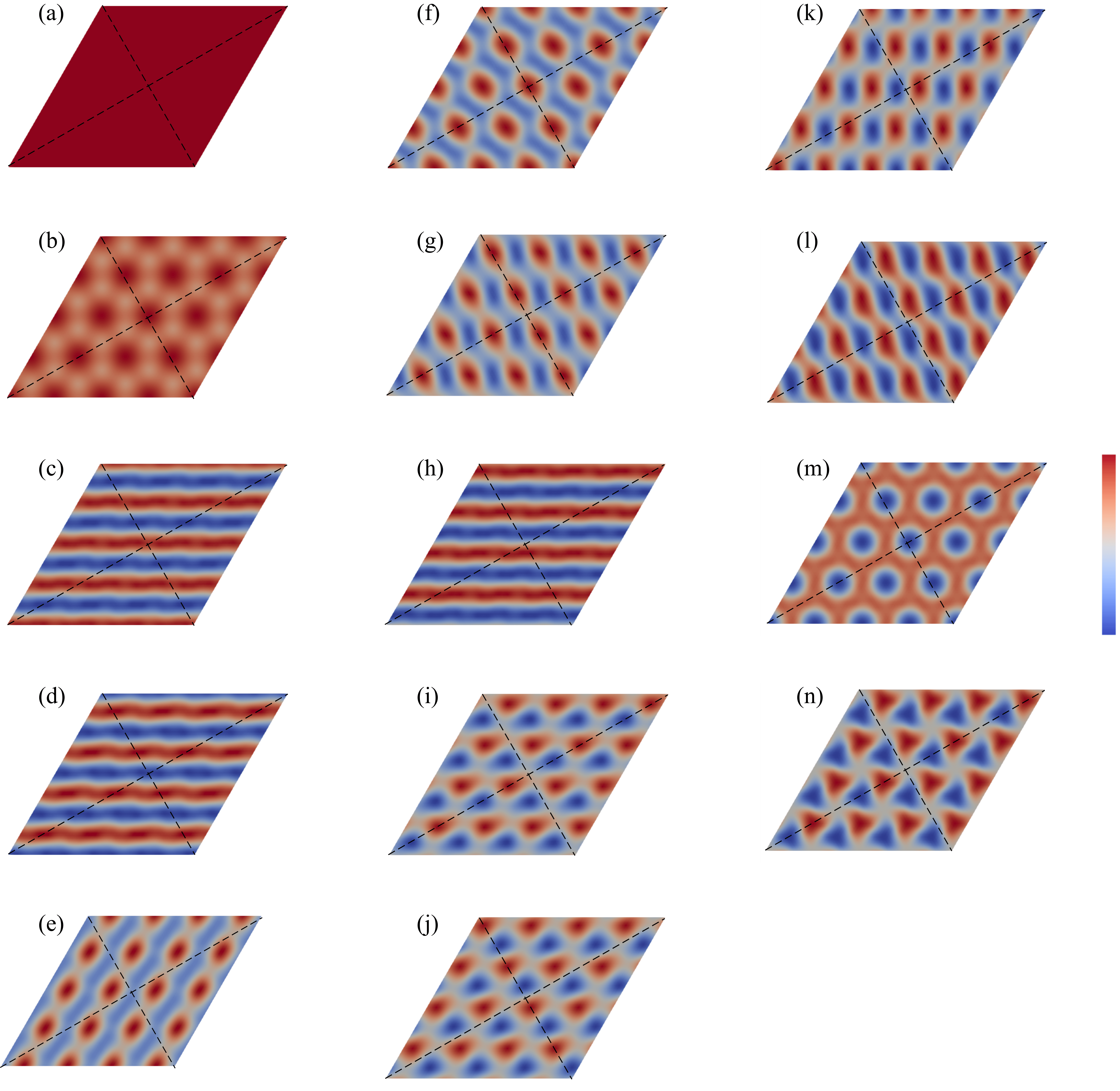
Figure 9: Nonzero projected Bloch mode shapes under rotation by $\theta=\pi$ in the top plate at $\Gamma$ point. Subfigures (a - n) correspond to modes (1 - 14). Modes having rotational eigenvalue $\lambda_{1}(p=1)$: 1-7, 13 and $\lambda_{2}(p=2)$: 8-12, 14. $(4\times 4)$ unit cells are shown for clarity of rotational symmetry.

Using the procedure in section III.2, the projected Bloch mode shapes $w^{p}_{\beta}(\bm{x})$ for the 14 modes below the band gap are determined at each of the high symmetry points. The non-zero projected mode shapes (real component) are presented in Figures 9 - 12. Only the top plate is shown although both plates are considered for determining the rotational eigenvalue $\lambda_{p}$ for each mode. The corresponding $\lambda_{p}$ for each mode are listed in the captions. Here, multiple unit cells are illustrated for clarity of the rotational symmetry. The rotation axis passes through the center, where the dashed lines intersect. For rotation about this axis by $\theta=\pi$, modes with rotational eigenvalue $\lambda_{1}$ will be symmetric. Similarly, for rotation by $\theta=2\pi/3$, the mode shapes with $\lambda_{1}$ will be unchanged after rotation.

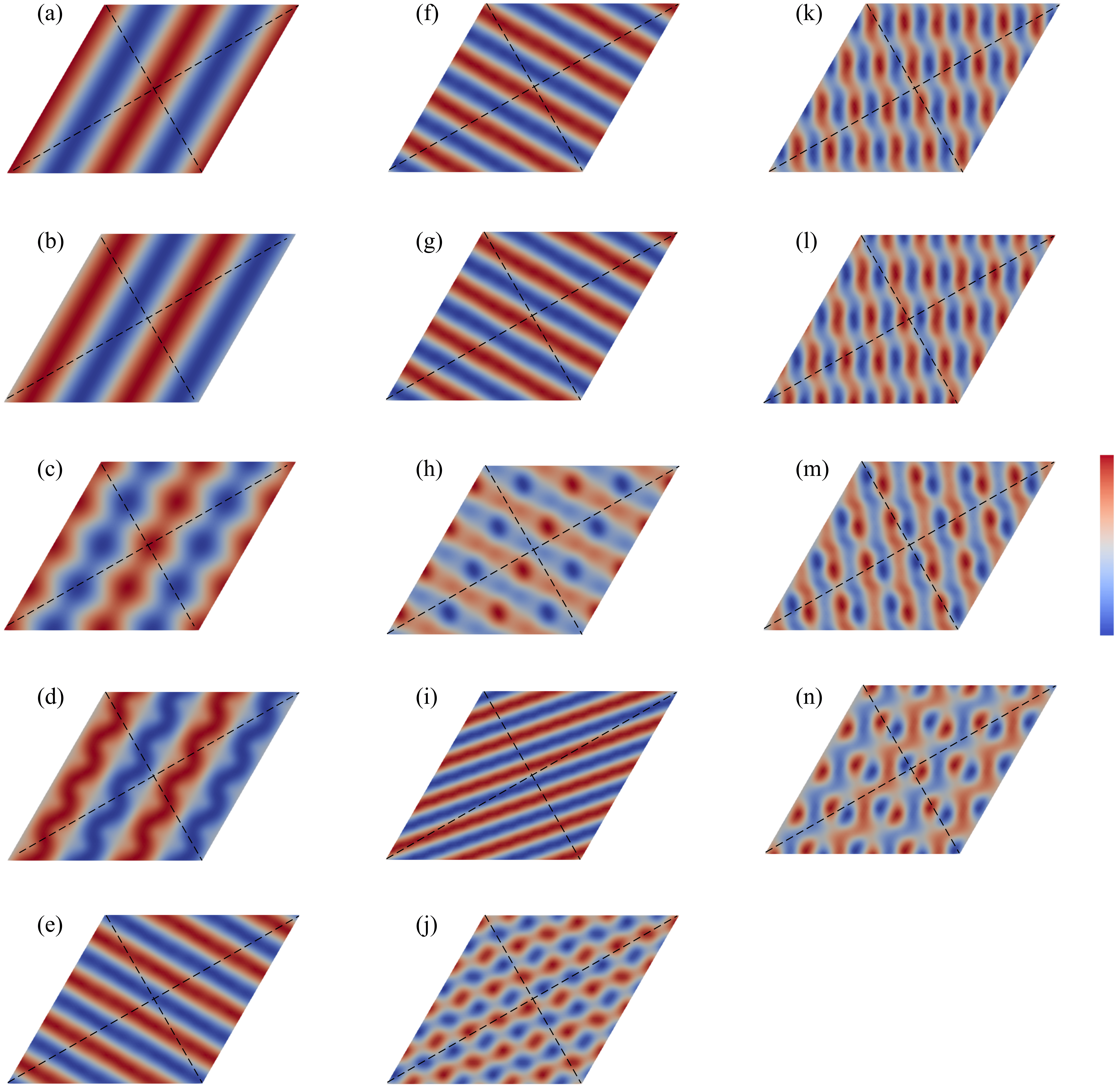
Figure 10: Nonzero projected Bloch mode shapes under rotation by $\theta=\pi$ in the top plate at $M$ point. Subfigures (a - n) correspond to modes (1 - 14). Modes having rotational eigenvalue $\lambda_{1}(p=1)$: $1,3,5,8,11,13$ and $\lambda_{2}(p=2)$: $2,4,6,7,9,10,12,14$. $(4\times 4)$ unit cells are shown for clarity of rotational symmetry.

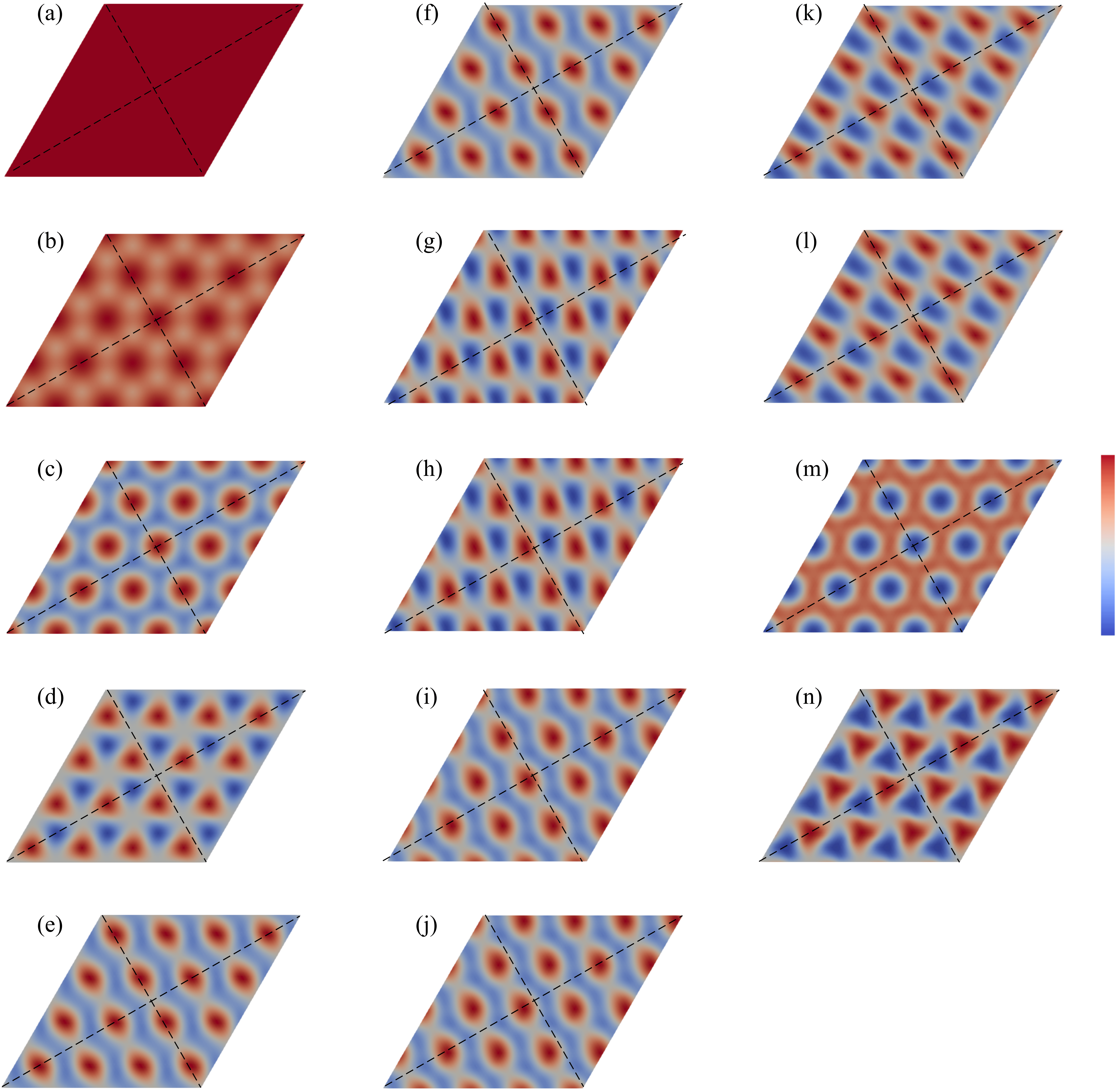
Figure 11: Nonzero projected Bloch mode shapes under rotation by $\theta=2\pi/3$ in the top plate at $\Gamma$ point. Subfigures (a - n) correspond to modes (1 - 14). Modes having rotational eigenvalue $\lambda_{1}(p=1)$: $1-4,13,14$, $\lambda_{2}(p=2)$: $5,7,9,11$ and $\lambda_{3}(p=3)$: $6,8,10,12$. $(4\times 4)$ unit cells are shown for clarity of rotational symmetry.

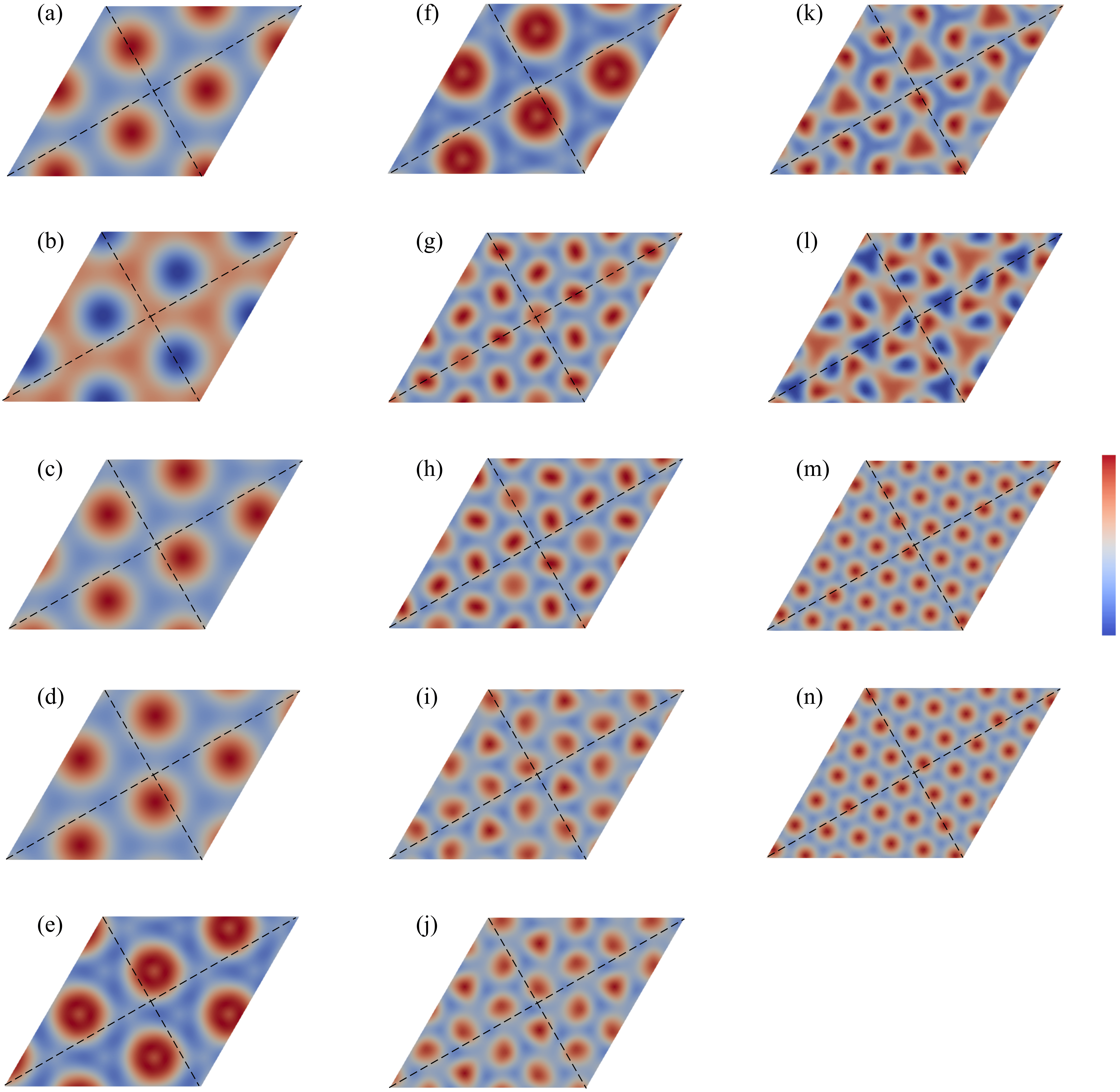
Figure 12: Nonzero projected Bloch mode shapes under rotation by $\theta=2\pi/3$ in the top plate at $K$ point. Subfigures (a - n) correspond to modes (1 - 14). Modes having rotational eigenvalue $\lambda_{1}(p=1)$: $1,2,7,8$, $\lambda_{2}(p=2)$: $3,5,9,11,13$ and $\lambda_{3}(p=3)$: $4,6,10,12,14$. $(4\times 4)$ unit cells are shown for clarity of rotational symmetry.

Appendix C Primitive generators and their fractional corner modes

We consider two primitive generators, identical to the ones introduced by Hughes and coworkers [22]. Figure 13(a,c) displays schematics of these lattices. The nodes have point masses with one degree of freedom and can move out-of-plane. The edges have linear springs with stiffness values either $k_{1}$ or $k_{2}$ as indicated. In both lattices, a nontrivial topological bandgap opens when $k_{1}<k_{2}$. The dispersion diagrams for these lattices, computed for $k_{1}=0.1$, $k_{2}=1.0$ and all unit masses, are displayed in Fig. 13(b,d).

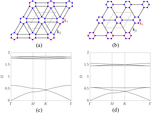
Figure 13: Schematic and dispersion diagram of the primitive generators. Schematic of (a) $h_{4b}$ and (d) $h_{3c}$ lattices. Unit cells are indicated by black dashed lines. Dispersion diagrams are shown along the IBZ boundary for (c) $h_{4b}$ and (d) $h_{3c}$ lattices.

The fractional corner modes at the corners of domains with 6-fold and 3-fold rotation symmetry are given by [22]

$$Q_{6} =\dfrac{[M_{1}^{(2)}]}{4}+\dfrac{[K_{1}^{(3)}]}{6}\mod 1$$ (26a)

$$Q_{3} =\dfrac{[K_{2}^{(3)}]}{3}\mod 1.$$ (26b)

Here $[K_{2}^{3}]$ is the difference between the number of modes at $K$ and $\Gamma$ points that have rotational eigenvalue $\lambda_{2}$. For each mode at the high symmetry points below the bandgap, the rotational eigenvalues are determined using the procedure discussed in Sec. III.2. For $h_{4b}$ lattice, the fractional corner mode values are

$$Q_{6} =\dfrac{(1-1)}{4}+\dfrac{(0-2)}{6}=-\dfrac{1}{3}\mod 1=\dfrac{2}{3}\mod 1,$$ (27a)

$$Q_{3} =\dfrac{(1-0)}{3}=\dfrac{1}{3}\mod 1,$$ (27b)

while for $h_{3c}$ lattice, they are

$$Q_{6} =\dfrac{(1-3)}{4}+\dfrac{(1-1)}{6}=-\dfrac{1}{2}\mod 1=\dfrac{1}{2}\mod 1$$ (28a)

$$Q_{3} =\dfrac{(1-1)}{3}=0.$$ (28b)

Appendix D Bulk and localized mode shapes

The complete mode shapes for the modes in Fig. 5 are presented. These include the top and bottom plate displacement contours, top and bottom layer resonator displacement contours. Note that there are two edge modes at the same frequency. Both mode shapes are illustrated below: subfigures (b, g) for one mode and (c, h) for the other.

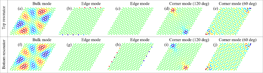
Figure 15: Displacement contours of top and bottom resonator for the same modes presented in Fig. 14. Top and bottom rows correspond to the top and bottom resonator displacement contours, respectively.

References

- Dos Santos et al. [2007] J. L. Dos Santos, N. Peres, and A. C. Neto, Graphene bilayer with a twist: Electronic structure, Physical review letters 99, 256802 (2007).
- Trambly de Laissardière et al. [2010] G. Trambly de Laissardière, D. Mayou, and L. Magaud, Localization of dirac electrons in rotated graphene bilayers, Nano letters 10, 804 (2010).
- Morell et al. [2010] E. S. Morell, J. Correa, P. Vargas, M. Pacheco, and Z. Barticevic, Flat bands in slightly twisted bilayer graphene: Tight-binding calculations, Physical Review B 82, 121407 (2010).
- Bistritzer and MacDonald [2011] R. Bistritzer and A. H. MacDonald, Moiré bands in twisted double-layer graphene, Proceedings of the National Academy of Sciences 108, 12233 (2011).
- Wang et al. [2012] Z. Wang, F. Liu, and M. Chou, Fractal landau-level spectra in twisted bilayer graphene, Nano letters 12, 3833 (2012).
- Cao et al. [2018] Y. Cao, V. Fatemi, S. Fang, K. Watanabe, T. Taniguchi, E. Kaxiras, and P. Jarillo-Herrero, Unconventional superconductivity in magic-angle graphene superlattices, Nature 556, 43 (2018).
- Gonzalez-Arraga et al. [2017] L. A. Gonzalez-Arraga, J. Lado, F. Guinea, and P. San-Jose, Electrically controllable magnetism in twisted bilayer graphene, Physical review letters 119, 107201 (2017).
- Dong et al. [2021] K. Dong, T. Zhang, J. Li, Q. Wang, F. Yang, Y. Rho, D. Wang, C. P. Grigoropoulos, J. Wu, and J. Yao, Flat bands in magic-angle bilayer photonic crystals at small twists, Physical review letters 126, 223601 (2021).
- Mao et al. [2021] X.-R. Mao, Z.-K. Shao, H.-Y. Luan, S.-L. Wang, and R.-M. Ma, Magic-angle lasers in nanostructured moiré superlattice, Nature nanotechnology 16, 1099 (2021).
- Oudich et al. [2021] M. Oudich, G. Su, Y. Deng, W. Benalcazar, R. Huang, N. J. Gerard, M. Lu, P. Zhan, and Y. Jing, Photonic analog of bilayer graphene, Physical Review B 103, 214311 (2021).
- Wang et al. [2020] P. Wang, Y. Zheng, X. Chen, C. Huang, Y. V. Kartashov, L. Torner, V. V. Konotop, and F. Ye, Localization and delocalization of light in photonic moiré lattices, Nature 577, 42 (2020).
- Wu et al. [2022] S.-Q. Wu, Z.-K. Lin, B. Jiang, X. Zhou, Z. H. Hang, B. Hou, and J.-H. Jiang, Higher-order topological states in acoustic twisted moiré superlattices, Physical Review Applied 17, 034061 (2022).
- Zheng et al. [2022] S. Zheng, J. Zhang, G. Duan, Z. Jiang, X. Man, D. Yu, and B. Xia, Topological network and valley beam splitter in acoustic biaxially strained moiré superlattices, Physical Review B 105, 184104 (2022).
- Yves et al. [2022a] S. Yves, Y.-G. Peng, and A. Alù, Topological lifshitz transition in twisted hyperbolic acoustic metasurfaces, Applied Physics Letters 121, 122201 (2022a).
- Jin et al. [2020] Y. Jin, W. Wang, Z. Wen, D. Torrent, and B. Djafari-Rouhani, Topological states in twisted pillared phononic plates, Extreme Mechanics Letters 39, 100777 (2020).
- López et al. [2020] M. R. López, F. Peñaranda, J. Christensen, and P. San-Jose, Flat bands in magic-angle vibrating plates, Physical Review Letters 125, 214301 (2020).
- López et al. [2022] M. R. López, Z. Zhang, D. Torrent, and J. Christensen, Theory of holey twistsonic media, Communications Materials 3, 99 (2022).
- Martí-Sabaté and Torrent [2021] M. Martí-Sabaté and D. Torrent, Dipolar localization of waves in twisted phononic crystal plates, Physical Review Applied 15, L011001 (2021).
- Oudich et al. [2022] M. Oudich, Y. Deng, and Y. Jing, Twisted pillared phononic crystal plates, Applied Physics Letters 120, 232202 (2022).
- Yves et al. [2022b] S. Yves, M. I. N. Rosa, Y. Guo, M. Gupta, M. Ruzzene, and A. Alù, Moiré-driven topological transitions and extreme anisotropy in elastic metasurfaces, Advanced Science 9, 2200181 (2022b).
- Benalcazar et al. [2017] W. A. Benalcazar, B. A. Bernevig, and T. L. Hughes, Quantized electric multipole insulators, Science 357, 61 (2017).
- Benalcazar et al. [2019] W. A. Benalcazar, T. Li, and T. L. Hughes, Quantization of fractional corner charge in c n-symmetric higher-order topological crystalline insulators, Physical Review B 99, 245151 (2019).
- Peng et al. [2022] Y. Peng, E. Liu, B. Yan, J. Xie, A. Shi, P. Peng, H. Li, and J. Liu, Higher-order topological states in two-dimensional stampfli-triangle photonic crystals, Optics Letters 47, 3011 (2022).
- Li et al. [2022] M. Li, Y. Wang, T. Sang, H. Chu, Y. Lai, and G. Yang, Experimental observation of multiple edge and corner states in photonic slabs heterostructures, Photonics Research 10, 197 (2022).
- Xiong et al. [2022] L. Xiong, Y. Liu, Y. Zhang, Y. Zheng, and X. Jiang, Topological properties of a two-dimensional photonic square lattice without c 4 and m x (y) symmetries, ACS Photonics 9, 2448 (2022).
- Wang et al. [2021a] H.-X. Wang, L. Liang, B. Jiang, J. Hu, X. Lu, and J.-H. Jiang, Higher-order topological phases in tunable c 3 symmetric photonic crystals, Photonics Research 9, 1854 (2021a).
- Wu et al. [2021] S. Wu, B. Jiang, Y. Liu, and J.-H. Jiang, All-dielectric photonic crystal with unconventional higher-order topology, Photonics Research 9, 668 (2021).
- Proctor et al. [2020] M. Proctor, P. A. Huidobro, B. Bradlyn, M. B. De Paz, M. G. Vergniory, D. Bercioux, and A. García-Etxarri, Robustness of topological corner modes in photonic crystals, Physical Review Research 2, 042038 (2020).
- Mizoguchi et al. [2020] T. Mizoguchi, Y. Kuno, and Y. Hatsugai, Square-root higher-order topological insulator on a decorated honeycomb lattice, Physical Review A 102, 033527 (2020).
- Wang et al. [2021b] Z. Wang, H. Li, Z. Wang, Z. Liu, J. Luo, J. Huang, X. Wang, R. Wang, and H. Yang, Straight-angled corner state in acoustic second-order topological insulator, Physical Review B 104, L161401 (2021b).
- Deng et al. [2022] Y. Deng, W. A. Benalcazar, Z.-G. Chen, M. Oudich, G. Ma, and Y. Jing, Observation of degenerate zero-energy topological states at disclinations in an acoustic lattice, Physical review letters 128, 174301 (2022).
- Yang et al. [2020] Z.-Z. Yang, X. Li, Y.-Y. Peng, X.-Y. Zou, and J.-C. Cheng, Helical higher-order topological states in an acoustic crystalline insulator, Physical Review Letters 125, 255502 (2020).
- Xue et al. [2019] H. Xue, Y. Yang, F. Gao, Y. Chong, and B. Zhang, Acoustic higher-order topological insulator on a kagome lattice, Nature materials 18, 108 (2019).
- Ni et al. [2019] X. Ni, M. Weiner, A. Alu, and A. B. Khanikaev, Observation of higher-order topological acoustic states protected by generalized chiral symmetry, Nature materials 18, 113 (2019).
- Serra-Garcia et al. [2018] M. Serra-Garcia, V. Peri, R. Süsstrunk, O. R. Bilal, T. Larsen, L. G. Villanueva, and S. D. Huber, Observation of a phononic quadrupole topological insulator, Nature 555, 342 (2018).
- Ezawa [2018] M. Ezawa, Higher-order topological insulators and semimetals on the breathing kagome and pyrochlore lattices, Physical review letters 120, 026801 (2018).
- Chen et al. [2022] Y. Chen, J. Li, and J. Zhu, Topology optimization of quantum spin hall effect-based second-order phononic topological insulator, Mechanical Systems and Signal Processing 164, 108243 (2022).
- Chen et al. [2021] C.-W. Chen, R. Chaunsali, J. Christensen, G. Theocharis, and J. Yang, Corner states in a second-order mechanical topological insulator, Communications Materials 2, 62 (2021).
- Danawe et al. [2021] H. Danawe, H. Li, H. Al Ba’ba’a, and S. Tol, Existence of corner modes in elastic twisted kagome lattices, Physical Review B 104, L241107 (2021).
- Ma et al. [2023] Z. Ma, Y. Liu, Y.-X. Xie, and Y.-S. Wang, Tuning of higher-order topological corner states in a honeycomb elastic plate, Physical Review Applied 19, 054038 (2023).
- Liu et al. [2023] Y. Liu, B. Lei, P. Yu, L. Zhong, K. Yu, and Y. Wu, Second-order topological corner states in two-dimensional elastic wave metamaterials with nonsymmorphic symmetries, Mechanical Systems and Signal Processing 198, 110433 (2023).
- Liu et al. [2021] B. Liu, L. Xian, H. Mu, G. Zhao, Z. Liu, A. Rubio, and Z. Wang, Higher-order band topology in twisted moiré superlattice, Physical Review Letters 126, 066401 (2021).
- Pal and Ruzzene [2017] R. K. Pal and M. Ruzzene, Edge waves in plates with resonators: an elastic analogue of the quantum valley hall effect, New Journal of Physics 19, 025001 (2017).
- Xiao et al. [2012] Y. Xiao, J. Wen, and X. Wen, Flexural wave band gaps in locally resonant thin plates with periodically attached spring–mass resonators, Journal of Physics D: Applied Physics 45, 195401 (2012).
- Torrent and Sánchez-Dehesa [2012] D. Torrent and J. Sánchez-Dehesa, Acoustic analogue of graphene: observation of dirac cones in acoustic surface waves, Physical review letters 108, 174301 (2012).
- Hasan and Kane [2010] M. Z. Hasan and C. L. Kane, Colloquium: topological insulators, Reviews of modern physics 82, 3045 (2010).
- Peterson et al. [2020] C. W. Peterson, T. Li, W. A. Benalcazar, T. L. Hughes, and G. Bahl, A fractional corner anomaly reveals higher-order topology, Science 368, 1114 (2020).
- Bradley and Cracknell [2010] C. Bradley and A. Cracknell, The mathematical theory of symmetry in solids: representation theory for point groups and space groups (Oxford University Press, 2010).
- Dresselhaus et al. [2007] M. S. Dresselhaus, G. Dresselhaus, and A. Jorio, Group theory: application to the physics of condensed matter (Springer Science & Business Media, 2007).
- Timoshenko et al. [1959] S. Timoshenko, S. Woinowsky-Krieger, et al., Theory of plates and shells, Vol. 2 (McGraw-hill New York, 1959).