Degree Distribution Identifiability of Stochastic Kronecker Graphs

Abstract

Large-scale analysis of the distributions of the network graphs observed in naturally-occurring phenomena has revealed that the degrees of such graphs follow a power-law or lognormal distribution. Some network or graph generation algorithms rely on the Kronecker multiplication primitive. Seshadhri, Pinar, and Kolda (J. ACM, 2013) proved that stochastic Kronecker graph (SKG) models cannot generate graphs with degree distribution that follows a power-law or lognormal distribution. As a result, variants of the SKG model have been proposed to generate graphs which approximately follow degree distributions, without any significant oscillations. However, all existing solutions either require significant additional parameterization or have no provable guarantees on the degree distribution.

• In this work, we present statistical and computational identifiability notions which imply the separation of SKG models. Specifically, we prove that SKG models in different identifiability classes can be separated by the existence of isolated vertices and connected components in their corresponding generated graphs. This could explain the large (i.e., $>50\%$) fraction of isolated vertices in some popular graph generation benchmarks.

• We present and analyze an efficient algorithm that can get rid of oscillations in the degree distribution by mixing seeds of relative prime dimensions. For an initial $2\times 1$ and $2\times 2$ seed, a crucial subroutine of this algorithm solves a degree-2 and degree-4 optimization problem in the variables of the initial seed, respectively. We generalize this approach to solving optimization problems for $m\times n$ seeds, for any $m,n\in{\mathbb{N}}$.

• The use of $3\times 3$ seeds alone cannot get rid of significant oscillations. We prove that such seeds result in degree distribution that is bounded above by an exponential tail and thus cannot result in a power-law or lognormal.

The definitions of identifiability of SKG models could lead to a better understanding and classification of graph generation algorithms.

1 Introduction

Graph models can be used to represent biological networks, social networks, communication networks, relationships between products and advertisers, and so on [14, 31, 36, 10, 28]. Representing these networks as graphs enables the mining of properties from these graphs [8]. However, companies that store large graph data, such as Netflix and Meta/Facebook, cannot share most of their graph data because of copyright, legal, and privacy issues [39, 9, 11]. As a result, a lot of research has been done to enable generation of graph models that realistically model “real-world” graphs, which should have an approximately lognormal or power law degree distribution [29]. The Stochastic Kronecker Graph (SKG) model has been proposed as a graph generation model and is currently employed by the Graph500 supercomputer benchmark, particularly because the SKG graph generation process is easily parallelized [13]. However, the original SKG model cannot generate a power law or even a log-normal distribution but instead is most accurately characterized as fluctuating between a lognormal distribution and an exponential tail [26]. Alternatives like the Noisy Stochastic Kronecker Graph model are also unsatisfactory partly due to their unwieldy additional parameterization [15].

We are thus motivated by the following questions posed by [41]:

What does the [degree] distribution oscillate between? Is the distribution bounded below by a power law? Can we approximate the distribution with a simple closed form function? None of these questions have satisfactory answers.

Instead of attempting to unconditionally show that certain SKG models have certain degree distributions in certain parameter regimes, we begin a systematic classification of SKG models. We view the model generating process through the lens of statistical and computational identifiablility [25, 1, 6].

Definition 1 presents a notion that can be used to classify when an SKG model or algorithm follows a certain distribution (e.g., lognormal or exponential). Definition 2 is the computational analogue. We conjecture that certain SKG models cannot be SKG-identifiable with certain parameterizations of the lognormal distribution while others can be. Then we discuss implications of these conjectures on the following graph properties: the existence of isolated vertices, the presence of connected components, and the degree distributions. As noted in previous work [41], the majority (i.e., $50-70\%$) of vertices in popular benchmark graphs are isolated. This is a major concern for such benchmarks since the generated graph would have a much smaller size than intended and the average degree would be higher than intended. Our work offers another view on the presence or absence of isolated vertices across benchmark graphs. Such graph generation algorithms belong in different identifiability classes since by Theorem 1, it is hard (in a precise sense) to identify seeds that generate graphs that do not have isolated vertices.

In addition, we present an algorithm that interpolates initiator seeds of different dimensions to generate graphs with no significant oscillations. We conjecture that SKG models require more than one $2\times 2$ seed to remove significant oscillations in the degree distribution. Evidence is presented to support this claim.

A SKG model is defined by an algorithm $\mathcal{A}$, an initiator set of seeds (usually a $2\times 2$ or $3\times 3$ matrix), and the target size of the graph. The Kronecker product is then applied to the seed to define a probability distribution over the resulting graph. See Sections 1.4 and 2 for more details on using the Kronecker multiplication primitive to generate a graph from a seed.

Intuitively, an SKG model is identifiable if there exists at least one distribution that is close to the degree distribution of the graph corresponding to an initiator seed. The model is computationally identifiable if, for any distribution, there exists an algorithm that will find such an initiator seed, that will correspond to the distribution, in a computationally-efficiently manner! A new approach to the classification and formalization of SKG models is necessary since it is not clear how to get rid of the significant variability in the degree distributions of the model. Furthermore, the identifiability criteria still carries over the benefits of existing SKG model variants (such as the Noisy SKG model and the Relative Prime Stochastic Kronecker Graph model, both of which we will discuss in detail in later sections). The separations of statistical and computational identifiability is also necessary because, except for ad-hoc and brute-force approaches, no feasible procedure is known to obtain or infer a seed that can be used to generate a graph with a certain degree distribution. Also, while the focus of existing SKG investigations has been on graphs with degree distributions that follow a power-law or lognormal measure, the definitions presented below aim to generalize the study of SKG target degree distributions.

For the definitions below, $\mathcal{P}(\Omega,\mathcal{F})$ is the set of all probability measures defined on $(\Omega,\mathcal{F})$.

Definition 1 (SKG Identifiable).

Fix $\alpha\geq 0$. Let $(\Omega,\mathcal{F})$ be a (Borel) measurable space and $\mathcal{D}$ be any probability measure or distribution defined on $(\Omega,\mathcal{F})$. For any $s\in{\mathbb{N}}$, consider $\mathcal{A}:{\mathbb{R}}^{s\times s}\times{\mathbb{N}}\rightarrow\mathcal{P}(\Omega,\mathcal{F})$, a (randomized) algorithm that outputs a degree distribution, given a set of seeds and target size of graph.

Then $\mathcal{A}$ is $\alpha$ SKG identifiable with distribution $\mathcal{D}$ if there exists a set of seeds $S$ such that for all $n\in{\mathbb{N}}$, $\mathrm{TV}(\mathcal{A}(S,n),\mathcal{D})\leq\alpha$.

For Definition 1, we do not need to require that $\mathcal{A}$ output a graph if it outputs a degree distribution since, up to isomorphisms, every degree distribution is realizable by a graph of a certain size. $\mathrm{TV}$ is the total variation distance (or statistical distance) between two distributions. Inspired by the computational analog of statistical distance (as introduced by Goldwasser and Micali [21, 20]), we introduce a computational analogue of identifiability of stochastic Kronecker graphs. We note that other statistical measures (e.g., max divergence or Rényi divergence) might be better at capturing tail behavior of distributions which could be quite interesting. We leave the exploration of such additional measures to future work.

Definition 2 (SKG Computationally Identifiable).

Let $\alpha(n)\geq 0$ be a sequence and let $(\Omega,\mathcal{F})$ be a (Borel) measurable space and $\mathcal{D}$ be any probability measure or distribution defined on $(\Omega,\mathcal{F})$ that can be represented by $\mathrm{poly}(n)$-bit strings. Let $\mathcal{B}=\{\mathcal{B}_{n}\}_{n\in{\mathbb{N}}}$ be a sequence of (randomized) algorithms that each can be represented by $\mathrm{poly}(n)$-bit strings. For any $s\in{\mathbb{N}}$ and $n\in{\mathbb{N}}$, consider $\mathcal{B}_{n}:{\mathbb{N}}\times\mathcal{P}(\Omega,\mathcal{F})\rightarrow{\mathbb{R}}^{s\times s}\times\mathcal{P}(\Omega,\mathcal{F})$, a (randomized) algorithm that, given any target size of graph and target distribution, can output a seed that can generate a graph with degree distribution that is close to the target.

Then $\mathcal{B}$ is $\alpha$ SKG computationally identifiable with distribution $\mathcal{D}$ if $\mathcal{B}$ runs in time $\mathrm{poly}(n,1/\alpha)$ and $\mathcal{B}(n,\mathcal{D})$ outputs a set of seeds $S$ and distribution $\mathcal{D}_{n}$ (representable by $\mathrm{poly}(n)$-bit strings) such that for all $n\in{\mathbb{N}}$, $\mathrm{TV}(\mathcal{D}_{n},\mathcal{D})\leq\alpha(n)$.

Definition 1 considers the existence of a seed that can be used to generate a graph with degree distribution that matches the target. To meet the definition, the algorithm is not required to find the seed. If such a seed exists, then a brute-force search over the domain of seeds, ${\mathbb{R}}^{s\times s}$, can be used to obtain such a seed. However, in Definition 2, we essentially restrict the set of algorithms to feasible algorithms that can find the seed that satisfies the distribution closeness requirement. That is, not only must the seed exist to generate the desired degree distribution but the algorithm must be able to find such a seed!

Definition 2 bears resemblance to a one-way function [22, 23]: it should be relatively easy to perform the stochastic Kronecker multiplication to generate a graph but obtaining the seed that would lead to any degree distribution should be computationally difficult. This simple observation leads to one of our conjectures and the resulting implication, which will be discussed in the next section.

To gain more intuition for statistical identifiability, consider Figure 1 that shows instantiations of the Relative Prime Stochastic Kronecker Graph (RPSKG ) algorithm (Algorithm 2) with different parameters. Clearly, one instantiation results in significant oscillations while the other does not. This shows a clear separation in the degree distributions of the generated graphs when different seed sets are used.

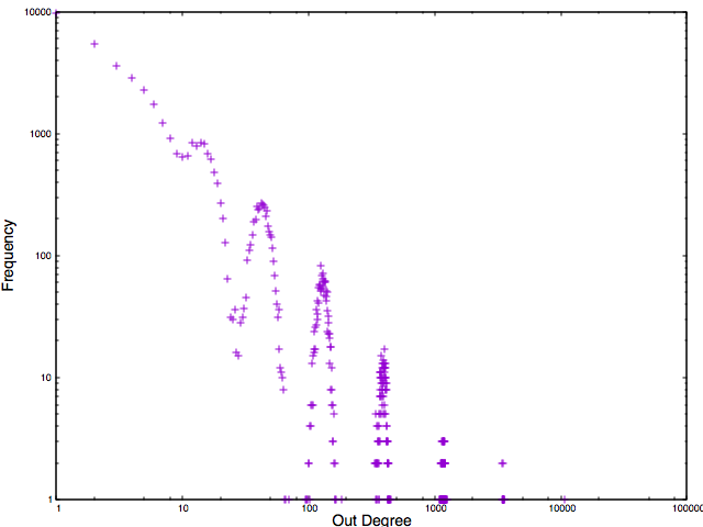
(a) ${\tt RPSKG}~{}(2^{20},16,0,T)$

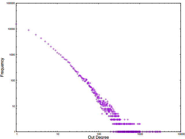
(b) ${\tt RPSKG}~{}(2^{20},15,1,T)$

Figure 1: Difference in degree distribution when only $2\times 2$ seeds are used (Figure 1(a)) versus when $3\times 3$ seeds are used with $2\times 2$ seeds (Figure 1(b)). The two algorithms belong in two different identifiability classes. See Section 5 for other simulation results.

1.1 Our Contributions

In our work, we use the statistical and computational identifiability notions to show separation of SKG models. The separability is achieved by the following criteria: the existence of isolated vertices and connected components in the generated graphs. In this work, we have focused on two prominent properties of generated graphs but we leave the exploration of other properties that exhibit separation to future work.

We conjecture that no (randomized) polynomial-time algorithm can identify a set of seeds (one or more) that will generate a graph with degree distribution that is close in statistical distance to any target distribution. It is straightforward to see that, in this case, the Kronecker multiplication primitive acts as a candidate one-way function. We also show that this implies that the algorithm cannot possibly be both SKG identifiable and generate graphs that have no isolated vertices (in the limit), even if such graphs exists. An analogous result holds for generating a connected graph.

Conjecture 1.

There always exists $n\in{\mathbb{N}}$, a degree distribution $\mathcal{D}$, and sequence $\alpha(n)\geq 0$ such that no polynomial-time algorithm $\mathcal{A}$ exists to find a set of seeds $S$ (independent of $n$), such that $\mathrm{TV}(\mathcal{A}(S,n),\mathcal{D})\leq\alpha(n)$.

Conjecture 1 can be used to show the following theorem:

Theorem 1 (Informal Version of Theorem 4).

Let $\mathcal{A}$ be a polynomial-time algorithm that can generate a graph, via a seed $S$, which follows a particular degree distribution for any node set size $n\in{\mathbb{N}}$.

Then, assuming Conjecture 1, there exists a degree distribution $\mathcal{D}$ and parameterized function $\alpha(n)\geq 0$ for which $\mathcal{A}$ will be unable to ensure that the generated graph has no isolated vertices while remaining $\alpha(n)$ SKG (statistically) identifiable, in the limit.

We also show a similar phenomenon for connected components in the generated graphs of the SKG model assuming Conjecture 1:

Theorem 2 (Informal Version of Theorem 6).

Let $\mathcal{A}$ be a polynomial-time algorithm that can generate a graph, via a seed $S$, which follows a particular degree distribution for any node set size $n\in{\mathbb{N}}$.

Then, assuming Conjecture 1, there exists a degree distribution $\mathcal{D}$ and parameterized function $\alpha(n)\geq 0$ for which $\mathcal{A}$ will be unable to ensure that the generated graph always has a connected component while remaining $\alpha(n)$ SKG (statistically) identifiable, in the limit.

We have established, via Theorems 1 and 2, the implications of not being able to identify starting seeds for any given graph. This is due to the computational limitations of classical computers so that it is not possible to efficiently find seeds that can generate a graph for any given degree distribution that always exhibits certain properties. However, are there even existing efficient algorithms that, given a seed, can generate desired distributions without oscillations? Algorithm 2 is one such candidate algorithm. It is able to mix $2\times 2$ and $3\times 3$ seeds to generate graphs with degree distributions that do not have undesirable oscillations. However, with only $3\times 3$ seeds, it still results in a distribution that is bounded above by an exponential tail. This result is proved in the following theorem:

Theorem 3 (Informal Version of Theorem 7).

There exists parameters $\alpha,\beta\in{\mathbb{N}}$ such that the degree of any vertex $v$ in the graph is

$$\mathbb{P}[\deg(v)=d]=(1\pm o(1))\frac{\exp(d(2\alpha+\beta)-e^{2\alpha+\beta})}{d!},$$

where $\deg(v)$ corresponds to the degree of vertex $v$.

Note that both $\alpha$ and $\beta$ are discrete (and not continuous) variables. As a consequence, the oscillations occur in the degree distribution. For example, when $|2\alpha+\beta-\ln d|\geq 1/3$, the probability of having degree $d$ is at most $\exp(-d/9)$, an exponential tail. But when $\ln d$ is close to integral, then there will be many vertices of degree $d$. Thus, there is a fluctuation in the degree distribution with exponential tails due to the discrete nature of the slice parameters, $\alpha$ and $\beta$. This reason is similar as why oscillations occur in the $2\times 2$ case.

This justifies the use of $2\times 2$ seeds together with $3\times 3$ seeds in Algorithm 2. Algorithm 2 is able to solve a degree-4 optimization problem in order to sample a $3\times 3$ seed from the uniform distribution over a given $2\times 2$ seed. Prior to our work, it was not known whether such an efficient procedure exists for the SKG model.

Lemma 1 (Informal Version of Lemma 6).

There exists a polynomial-time degree-4 optimization formulation to sample an SKG $3\times 3$ seed from the uniform distribution over a $2\times 2$ seed.

Lemma 2 (Informal Version of Lemma 5).

There exists a polynomial-time degree-2 optimization formulation to sample an SKG $3\times 1$ seed from the uniform distribution over a $2\times 1$ seed.

Also, as we show, Algorithm 2 can also be generalized to sample a $m\times n$ seeds for any $m,n\in{\mathbb{N}}$. See Section 4.1 for more details.

The second conjecture states that a $2\times 2$ set of seeds alone or $3\times 3$ set of seeds alone is not sufficient to generate graphs with no oscillations in the degree distribution. (See Section 5 for full experimental validation details.) As can be seen in Figure 1, this conjecture is supported by experiments. In particular, the generation process for Figure 1(a) uses only one $2\times 2$ set of seeds while the generation process for Figure 1(b) uses one set of $2\times 2$ seeds and one set of $3\times 3$ seeds.

Conjecture 1 implies the existence of one-way functions and cryptographic pseudorandom generators with seed length $d(m)<m$. This is because $\mathcal{D}$ can be chosen to be any distribution, representable with $\mathrm{poly}(n)$-bit strings, and so if the seed $S$ (which could be standardized to be of any length) cannot be found by polynomial-time algorithms, the Kronecker multiplication primitive (on the seed) would serve as a one-way function for which no efficient algorithms exist to find the seed.

Now we present the conjecture that is supported by a swath of experimental details (see Section 5):

Conjecture 2.

For all $\alpha>0$ and renormalized seed sets from either ${\mathbb{Q}}_{+}^{2\times 2}$ or ${\mathbb{Q}}_{+}^{3\times 3}$, there always exists a distribution $\mathcal{D}$ such that for all algorithms $\mathcal{A}$, $\mathrm{TV}(\mathcal{A}(S,n),\mathcal{D})>\alpha$.

In other words, to generate a graph with degree distribution in any possible identifiability class, an SKG algorithm cannot do so with only a $2\times 2$ set of seeds or a $3\times 3$ set of seeds. This observation is supported by empirical evidence and a new algorithm that can combine different seed sets. In Conjecture 2, renormalized seed sets refer to sets for which all entries are divided by the total sum so that it corresponds to a probability vector.

In Section 4, we come up with a new proposal to eliminate oscillations in any degree distribution generated by stochastic Kronecker multiplications. The ${\tt RPSKG}~{}$ algorithm works by using a $2\times 2$ seed matrix and $3\times 3$ seed matrix to generate the graph. We show that this eliminates oscillations in the degree distributions (unlike SKG). Also, the Noisy SKG proposal implicitly combines a $2\times 2$ seed matrix with another seed matrix to remove oscillations in the degree distribution  [41].

In this work, we focus on analyzing properties of SKG-generated graphs like connectedness, the existence of isolated vertices, and the degree distributions. As we show, there might be phase transitions in SKG identifiability via a threshold value [5, 16, 17]. Furthermore, the separations might be able to import some recent understanding in the theory of stochastic block models [4, 2, 3], a study we leave for future work.

1.2 Overview of Techniques

1.2.1 First and Second Moment Methods

To prove Theorems 4 and  6, we construct a sequence of pair of graphs for which their degree distributions satisfy a statistical distance upper bound that is a function of $\alpha(n)\geq 0$. Then we consider the event that a vertex is isolated. We prove that, over the entire graph, for one sequence of graphs, $\mathbb{P}[\exists\,\,\text{isolated nodes}]$ goes to 0 and for the other sequence, it goes to 1. For one sequence of graphs, we only consider the first moment of the random variable that counts the number of isolated vertices. For the second sequence of graphs, we consider the second moment of the random variable.

1.2.2 The RPSKG algorithm

Algorithm 2 is able to generate a graph without oscillations (as detailed in Section 5). The algorithm mixes the use of $2\times 2$ with $3\times 3$ seeds. A subroutine samples a $3\times 3$ seed from the uniform distribution over the $2\times 2$ seed. We show that this sampling problem corresponds to solving a degree-4 optimization problem in the variables of the $2\times 2$ seed. Also, even though Algorithm 2 is written in a serial form for clarify sake, it is easy to see that it is easily parallelizable.

1.3 Why is a New Approach Necessary and Important?

Graph analysis remains important and relevant. On one hand, we need to design efficient algorithms to infer properties from these large “real-world” graphs. As a result, a lot of research has been done to enable generation of graph models that realistically model “real-world” graphs. The celebrated work of Erdős and Rényi  [18, 19] for fast construction of random graphs just by inserting each edge with probability $p>0$ does not seem to be a good solution in this context, since social graphs have many properties (for example triadic closure and homophily) that random graphs don’t model well. Thus, a more realistic model is needed. The model that is usually used in practice is the Stochastic Kronecker Model (SKG) proposed in 2010 by Leskovec et al. [30] (further discussed in Section 2.1). This model has been chosen to create graphs for the Graph500 supercomputer benchmark  [13]. SKG models are used for various reasons: it has very few parameters and can generate graphs fully in parallel — on a per-edge basis.

However, the SKG model has several problems that differentiate its generated graphs from real network structures (social networks, for instance). In particular, Seshadhri et al.  [41] proved that SKG models cannot generate a power law or log-normal distribution. Graphs generated by the Stochastic Kronecker Graph model is most accurately characterized as fluctuating between a log-normal distribution and an exponential tail. Figure 1(a) is an example of a plot (on a log-log scale) of the degree distribution of a graph generated by SKG. This figure clearly shows unwanted oscillations in the degree distribution. The Noisy Stochastic Kronecker Graph (NSKG) model attempts to fix some of the problems with the SKG model. The main problem NSKG fixes is that it gets rid of the oscillations in the degree distributions of generated graphs. However, NSKG generates multiple random numbers that scales proportionally (logarithmically) with the number of edges generated. These random numbers are additional parameter artifacts that must be recorded for reproducibility sake, thus making NSKG unwieldy.

In this paper, we present a new model, the Relative Prime Stochastic Kronecker Graph (RPSKG ) model, that can generate graphs with log-normal degree distributions that do not have unwanted oscillations (unlike SKG) while adding no additional parameters (unlike NSKG). In addition, we present theoretical and experimental results about the RPSKG model that show its superiority to SKG.

The main contribution of our paper, though, is in presenting criteria (via definitions of statistical and computational identifiability) to classify and separate SKG models. The implications of the conjectures show the necessity of the classification of SKG models. The RPSKG model is a family of algorithms that is adaptive to interpolation of seeds of different dimensions. We believe this model and the ${\tt RPSKG}~{}$ algorithm warrants further study.

1.4 Additional Notation and Background

In Section 2, we dive into contextual work related to our research but first we introduce some preliminary notation that will be useful throughout this paper.

The SKG, NSKG, and RPSKG models all belong to a family on Kronecker models that rely on a non-traditional matrix operation, the Kronecker product (otherwise known as the Tensor product). The Kronecker product of two matrices $A\in\mathbb{R}^{m\times n}$, $B\in\mathbb{R}^{p\times q}$ is an $mp\times nq$ matrix, defined as follows:

$$A\otimes B=\begin{bmatrix}a_{11}B&\cdots&a_{1n}B\\ \vdots&\ddots&\vdots\\ a_{m1}B&\cdots&a_{mn}B\\ \end{bmatrix}=\begin{bmatrix}a_{11}b_{11}&\cdots&a_{1n}b_{1q}\\ \vdots&\ddots&\vdots\\ a_{m1}b_{p1}&\cdots&a_{mn}b_{pq}\\ \end{bmatrix}$$

Also common to the three models is a initiator matrix, which is usually a $2\times 2$ matrix. The Kronecker power of this matrix is then computed until we obtain a (usually large) matrix with dimensions of an adjacency matrix of the the graph we wish to generate. The generated matrix is a probability matrix (all values sum to one if the matrices involved in the product also have values that sum to one) which we can sample from to generate edges. Thus, we use this matrix to generate edges for a graph.

In practice, we do not actually generate this large matrix but simulate its generation for use in sampling on a per-edge basis. In addition to the initiator matrix, the models require a parameter for the number of Kronecker products performed. In both NSKG and SKG, $\ell$ is the number of Kronecker products. As a consequence, the number of nodes generated depends on $\ell$. For both NSKG and SKG, $2^{\ell}$ nodes are generated. On the other hand, for RPSKG , the number of nodes generated is $3^{k}\cdot 2^{\ell}$ where $k$ is the number of $3\times 3$ seeds used. Refer to Algorithm 2 for a description of the use of the seeds. Note that, via standard rounding techniques, the generation process can be adjusted to generate any number of nodes.

The SKG is not only a theoretical model; it is heavily used in practice as well. For example, the Graph500 supercomputer benchmark uses SKG with the following initiator matrix

$$T=\begin{bmatrix}t_{1}&t_{2}\\ t_{2}&t_{3}\\ \end{bmatrix}=\frac{1}{16}\begin{bmatrix}9&3\\ 3&1\\ \end{bmatrix}$$ (1)

and generates graphs with $m=16\cdot 2^{\ell}$ edges, $n=2^{\ell}$ nodes where $\ell\in\{26,29,32,36,39,42\}$.

Notice that the Graph500 initiator matrix in Equation 1 is symmetric. Often times, in other situations, this matrix is symmetric. We exploit this property in our theoretical analysis. We now precisely define the stochastic Kronecker graph model:

Definition 3 (Stochastic Kronecker Graph).

A Stochastic Kronecker Graph (SKG) is defined by an integer $\ell$ and a matrix $S\in{\mathbb{R}}^{s\times s}$ for some $s\in{\mathbb{N}}$. $S$ is the base or initiator matrix.

The graph generated will have $n=s^{\ell}$ vertices, where each vertex is labeled by a unique bit vector of length $\ell$. Given two vertices $u$ (with label $u_{1}u_{2}\ldots u_{\ell}$) and $v$ (with label $v_{1}v_{2}\ldots v_{\ell}$) the probability of the edge $(u,v)$ appearing in the resulting graph is $\prod_{i}^{\ell}S[u_{i},v_{i}]$, independent of the presence of other edges.

Often, the Stochastic Kronecker Graph definition (Definition 3) is assumed to rely on $2\times 2$ seed matrices to generate the graph. We generalize this notion to allow for seeds of any dimension. Also, although the number of edges in the generated graph is often variable, we can also impose a restriction on the number of edges. e.g., by sampling from a truncated distribution like the truncated normal and using rounding techniques. As we will discuss, Definition 3 is inspired by the Recursive Matrix model [24].

2 Related Work

In this section, we survey some graph generation models and will focus on discussing SKG, NSKG, and Multiplicative Attribute Graph models. Also, we discuss some of the work done in the validation of graph generation models. See works of Margo [32] for a more complete survey.

2.1 Stochastic Kronecker Graphs

In a seminal paper, Leskovec et al. [30] define the Stochastic Kronecker Graph (SKG) model that can be very effective in capturing the characteristics of real social networks (for example, small diameters and heavy-tailed degree distributions).

The SKG model is a generalization of the Recursive Matrix model introduced by Chakrabarti et al. [15]. To generate a Stochastic Kronecker graph, they use a single $K\times K$ initiator matrix $T$. Often $K=2$, a model equivalent to R-MAT [24]. Each of the $K^{2}$ entries in the initiator matrix represents the probability of generating an edge for a specific source and target vertex regions of the graph. For example, for the Graph500 benchmark $2\times 2$ seed matrix (Equation 1), the seed values mean that there is roughly a $56\%$ chance of inserting an edge in the top-left quadrant of the generated graph. The resulting graph can be naively generated by the Kronecker product as follows:

$$P=T^{\otimes\ell}=T\otimes T\otimes\ldots\otimes T=T^{\otimes\ell-1}\otimes T$$

In the resulting matrix, $P_{ij}$ represents the probability that there is an edge connecting the nodes $i$ and $j$. In practice, the Kronecker is simulated by recursively choosing a sub-region of matrix $T^{\otimes r}$ (after $r\leq\ell$ steps) until we descend on a single cell of $P$ and then place an edge. To further illustrate the generation process, suppose we use a $2\times 2$ initiator matrix and wish to generate graph on $m=16\cdot 2^{\ell}$ (often used in practice—for Graph500 for example). Then for every edge, we divide the adjacency matrix into four quadrants, and choose one of them with the corresponding probability that the $2\times 2$ seed matrix suggests. Once a quadrant is chosen, this procedure is repeated recursively. Intuitively, if we consider the indices of the vertices to be binary numbers, the $r^{th}$ step of this process fixes the $r$th most important bit of the two endpoints of the edge. Note that, using this approach some of the edges may be inserted multiple times. According to experiments, however, this occurs rarely — less that 1% of the total number of edges. One of the most important characteristics of this model, that makes it widely applicable in practice, is that it can generate graphs fully in parallel. Because of this property, the Graph500 supercomputer benchmark uses SKG by default to generate large graphs. Although the SKG model has been influential and is widely used in practice, there are several problems with the model:

1. The degree distribution of the generated graph does not have the wanted heavy-tail behavior but there are large oscillations instead. First, Grőer et al. [24] proved that the degree distribution behaves like a sum of Gaussians and later Seshadhri et al. [41] showed that it oscillates between a log-normal distribution and an exponential tail.

2. A very large fraction of the vertices of every graph is isolated and thus the graphs created with this model have a much smaller size and are much more dense than expected.

3. The max core numbers in the generated graphs are extremely small — much smaller than those corresponding of real graphs.

Taking these problems into consideration, one would like to improve this model in order to keep the easy generation and parallelization but make behave it more like real-life graphs. In Section 2.2, we briefly discuss the fix that was proposed by Seshadhri et al. [41] and note some potential problems. In Section  4, we come up with a new proposal to eliminate the oscillations in the degree distribution and subsequently validate our proposal theoretically and experimentally.

Mahdian et al. [37] show necessary and sufficient conditions for stochastic Kronecker graphs to be connected or to have giant components of size $\Theta(n)$ with high probability. They study the connectivity and searchability probabilities of both random graphs (a generalization of the Erdős-Rényi model) and stochastic Kronecker graphs.

Mihyun Kang et al. [27] also examine properties of stochastic Kronecker graphs but focus more on on showing that the graphs do not feature a power law degree distribution nor a log-normal degree distribution.

2.2 Noisy Stochastic Kronecker Graphs

Seshadhri et al. [41] provide rigorous proofs for many of the problems with the SKG model (stated previously in Section 2.1). In addition, Seshadhri et al. provide a new model — the Noisy SKG — that fixes some of the problems with the original SKG model. The idea is to add noise in every step of the computation (i.e., of the edge creation) so that edges are not sampled from the actual distribution created by the initial $2\times 2$ seed matrix, but rather from a noisy version of it. At each step $r\leq\ell$ of the recursive generation of the Kronecker product, $\mu_{r}$ is the noise factor chosen from the uniform distribution with range $[-b,+b]$ where $b\leq\min(t_{2},(t_{1}+t_{4})/2)$ is the noise parameter. The initiator matrix $T$ is transformed on a per-level basis to become:

$$\begin{bmatrix}t_{1}-\frac{2\mu_{r}t_{1}}{t_{1}+t_{4}}&t_{2}+\mu_{r}\\ t_{3}+\mu_{r}&t_{4}-\frac{2\mu_{r}t_{4}}{t_{1}+t_{4}}\\ \end{bmatrix}$$

Although, the generated graph of NSKG models are an improvement over SKG models, there are still some problems with the NSKG model:

1. Adding too much noise could destroy some “real-world” properties of the graph. In a sense, adding noise is equivalent to superimposing an Erdős-Rényi graph on the Kronecker graph. The larger the noise, the quicker the generated graph converges to a random graph.

2. During and after graph generation, we have to keep track of the $\ell$ random $\mu_{r}$ $(1\leq r\leq\ell)$ used for noise thus adding to our already cumbersome parameter list.

3. The large amount of noise added could sometimes make the generated graphs significantly different from others generated using the same initiator matrix. Therefore, to make safe conclusions about experiments based on the generated graphs, users must generate many such graphs thereby adding to the computation cost (e.g., supercomputing cost for Graph500).

4. Related to our previous point, since the noise is white (i.e., its expectation is 0) if we create several graphs, on average we expect that our results would not be noisy, and thus the oscillations in the degree distribution will reappear. This means that although the degree distribution of every graph is log-normal, the degree distribution of the whole family of graphs is still oscillating between a log-normal and an exponential tail.

We would like to note that although the NSKG model was communicated to the Graph500 committee, it is not used in the standard and is in fact compile-time disabled by default. This might imply that the Graph500 committee had some concerns (probably similar to ours) about the NSKG model.

2.3 Multiplicative Attribute Graph Model

Kim and Leskovec [26] present the Multiplicative Attribute Graph (MAG) model which is very similar to SKG. MAG models are essentially a generalization of SKG where each level (for generating a single edge) may have a different matrix $T$ (denoted $\Theta$ in their paper). The $\Theta$ matrices are the link-affinity matrices that be used to model link structure between nodes. Kim and Leskovec show that certain configurations of these matrices can lead to power-law or log-normal distributions.

However, MAG models are more complex than the family of Stochastic Kronecker Graph models as each node stores attributes and the different link-affinity matrices add complexity to the model specification.

2.4 Validation of Degree Distributions

We agree with Mitzenmacher  [35] with the sentiment that in studying power-law (and related) distributions of graph models we should not only observe, interpret, and model but also aim to validate and control our research. As a consequence, we do not just present our algorithm but show through experiments (in Section 5) that graphs generated by RPSKG approximately follow a log-normal distribution.

According to Newman [38], distributions that follow log-normal typically arise when multiplying random numbers. Mitzenmacher [34] uses the term multiplicative process to describe this model. The log of the product of a large number of random numbers is the sum of the logarithms of those same random numbers, and by the central limit theorem such sums have a normal distribution essentially regardless of the distribution of the individual numbers.

Furthermore, Mitzenmacher describes some generative models for power law and log-normal distributions [34]. Specifically, he describes how the preferential attachment models leads to a power law distribution. In preferential attachment models, new objects tend to attach to popular objects. In the case of the Web graph, new links tend to go to pages that already have links.

2.5 Relation to the Chung-Lu Model

We also note that the SKG model is related to other graph models. We cannot possibly exhaustively relate to every other possible graph generation model but will focus on one other: the Chung-Lu model. In [40], Seshadhri, Pinar, and Kolda explore similaries between SKG models and the Chung-Lu model.

Let $d_{1},d_{2},\ldots,d_{n}$ be a sequence of $n$ in-degrees and $d_{1}^{\prime},d_{2}^{\prime},\ldots,d_{n}^{\prime}$ be a sequence of $n$ out-degrees such that $\sum d_{i}=\sum d_{i}^{\prime}=m$. Then consider the probability matrix $P_{CL}$ for making $m$ edge insertions: the $(i,j)$th entry is $d_{i}d_{j}^{\prime}/m^{2}$. In the Chung-Lu model, $P_{CL}$ is used to generate the graph and can be used to model any degree distribution [12].

3 Existence of Isolated Vertices and Connected Components

Conjecture 1 separates statistical and computational SKG identifiability. In particular, as we will show, if the (poly-time) algorithm cannot find a seed that will follow a specific degree distribution, the algorithm cannot ensure certain properties of the graph. Specifically, even if a graph—which follows a certain degree distribution up to statistical distance— without any isolated vertices exists, the algorithm will be unable to generate such a graph.

There could be other ramifications of the separations of statistical and computational identifiability in terms of graph properties. We first consider a most obvious one — existence of isolated vertices.

3.1 Isolated Vertices

Our work shows a threshold phenomena for the existence of isolated nodes. The function $\alpha(n)\geq 0$ can be thought of as one with arbitrarily slow growth to infinity. For example, $\alpha(n)=\log\log\log n$.

Theorem 4.

Let $\mathcal{A}$ be a polynomial-time algorithm that can generate a graph, via a seed $S$, which follows a particular degree distribution for any node set size $n\in{\mathbb{N}}$.

Then assuming Conjecture 1, there exists a degree distribution $\mathcal{D}$ and $\beta(n)\geq 0$ for which $\mathcal{A}$ will be unable to ensure that the generated graph has no isolated vertices while remaining $\beta(n)$ SKG statistically identifiable, in the limit.

Proof.

Without loss of generality, we will consider the uniform degree distribution since for any random variable $X$ with CDF $F_{X}$, we can transform to a uniformly distributed random variable via $F_{X}(X)$.

Consider the uniform degree distribution generated by a homogeneous Bernoulli graph: each graph sequence $G_{n}$ has probability of $p_{n}$ of any two nodes having an edge. Then by Lemma 3, if $p_{n}$ is above some threshold, $\mathbb{P}(\exists\text{ isolated nodes})\rightarrow 0$. If $p_{n}$ is below some threshold, $\mathbb{P}(\exists\text{ isolated nodes})\rightarrow 1$.

By the conjecture, since the algorithm is bounded by a polynomial-time runtime, it cannot distinguish between two seeds $T_{1}$ and $T_{2}$, exactly one of which generates a graph without isolated nodes (in the limit). Moreover, the edge link probabilities of the two graphs are chosen to be within $2\alpha(n)/n$ to induce closeness in degree distributions. In particular, the TV distance between the distributions of the two generated graphs is at most $\beta(n)\leq\alpha(n)$.

As a result, by Lemma 3, the algorithm $\mathcal{A}$ cannot ensure the generated graph is SKG statistically identifiable and has no isolated vertices.

∎

Lemma 3.

Fix $s\in{\mathbb{N}}$ and let $T_{1},T_{2}\in{\mathbb{R}}^{s\times s}$ be two SKG seeds. Let $\alpha(n)\geq 0$ be a sequence that depends on $n$. Then let $T_{1}^{\otimes\ell}$ produce a $n$-node graph $G_{1}$ with (homogeneous) link probability of $p_{n}\geq\frac{\log n+\alpha(n)}{n}$. And let $T_{2}^{\otimes\ell}$ produce a $n$-node graph $G_{2}$ with (homogeneous) link probability of $p_{n}\leq\frac{\log n-\alpha(n)}{n}$.

Then

$$\mathbb{P}[\exists\text{ isolated nodes in }G_{1}]\rightarrow 0,$$

$$\mathbb{P}[\exists\text{ isolated nodes in }G_{2}]\rightarrow 1.$$

Furthermore,

$$\mathbb{E}[\text{isolated nodes in }G_{1}]\leq e^{p_{n}}e^{-\alpha(n)}.$$

Proof.

Consider the $n$ nodes of a graph $G_{n}$: $v_{1},v_{2},\ldots,v_{n}$. Let $E_{i}$ denote the event that any vertex $v_{i}$ is isolated. The the number of isolated vertices in $G_{n}$ is

$$X_{n}=\sum_{i=1}^{n}\mathds{1}[E_{i}].$$

The probability of the event $E_{i}$ is $(1-p_{n})^{n-1}$ (using independence and since w.p. at least $1-p_{n}$, any vertex is not connected to any others). Then

$$\mathbb{E}[X_{n}]=\sum_{i=1}^{n}\mathbb{E}[\mathds{1}[E_{i}]]=\sum_{i=1}^{n}\mathbb{P}[E_{i}]=n(1-p_{n})^{n-1}.$$ (2)

Using the taylor expansion of $\log(1-t)=-\sum_{k=1}^{\infty}\frac{t^{k}}{k}$, it can be derived that

$$\log(1-t)\leq-t,\quad\forall t\in[0,1).$$ (3)

Furthermore,

$$\log(1-t)\geq-t-t^{2},\quad\forall t\in[0,1/2].$$ (4)

Case (i): For graphs of type $G_{1}$, we have $p_{n}\geq\frac{\log n+\alpha(n)}{n}$ for some $\alpha(n)\rightarrow\infty$. Then by Equation 2 and Equation 3:

$$\mathbb{E}[X_{n}] =e^{\log n+(n-1)\log(1-p_{n})}$$ (5)

$$\leq e^{\log n-(n-1)p_{n}}$$ (6)

$$=e^{p_{n}}e^{\log n-np_{n}}$$ (7)

$$\leq e^{p_{n}}e^{-\alpha(n)}.$$ (8)

So, $\mathbb{E}[\text{isolated nodes in }G_{1}]\leq e^{p_{n}}e^{-\alpha(n)}$ and by Markov’s inequality,

$$\mathbb{P}[\exists\text{ isolated nodes in }G_{1}]=\mathbb{P}(X_{n}\geq 1)\leq\mathbb{E}[X_{n}]\rightarrow 0.$$

Case (ii): We will consider graphs of type $G_{2}$ and apply Chebyshev’s inequality as follows:

$$\mathbb{P}(X_{n}=0) \leq\mathbb{P}(X_{n}\leq 0)$$ (9)

$$\leq\mathbb{P}(|X_{n}-\mathbb{E}[X_{n}]|\geq\mathbb{E}[X_{n}])\leq\frac{\mathrm{Var}(X_{n})}{(\mathbb{E}[X_{n}])^{2}}.$$ (10)

For graphs of type $G_{2}$, $p_{n}\leq\frac{\log n-\alpha(n)}{n}$ for some $\alpha(n)\rightarrow\infty$. Clearly, for large $n$, $p_{n}\leq 1/2$. Then by Equation 2 and Equation 4:

$$\mathbb{E}[X_{n}] =e^{\log n+(n-1)\log(1-p_{n})}$$ (11)

$$\geq e^{\log n-(n-1)(p_{n}+p_{n}^{2})}$$ (12)

$$\geq e^{\log n-np_{n}-np_{n}^{2}}.$$ (13)

Since $np_{n}\leq\log n-\alpha(n)$ and $np_{n}^{2}=1/n\cdot(np_{n})^{2}\leq 1/n\cdot(\log n)^{2}\leq 1$, then as $n\rightarrow\infty$,

$$\mathbb{E}[X_{n}]\geq e^{\alpha(n)-1}\rightarrow\infty.$$

Next we analyze the variance:

$$\mathbb{E}[X_{n}^{2}]=\mathbb{E}\left[\sum_{i=1}^{n}\sum_{j=1}^{n}\mathds{1}[E_{i}]\mathds{1}[E_{j}]\right]=\sum_{i=1}^{n}\sum_{j=1}^{n}\mathbb{P}(E_{i},E_{j}).$$

Then

$$\mathrm{Var}(X_{n})=\mathbb{E}[X_{n}^{2}]-(\mathbb{E}[X_{n}])^{2}=\sum_{i=1}^{n}\sum_{j=1}^{n}\left(\mathbb{P}(E_{i},E_{j})-\mathbb{P}(E_{i})\mathbb{P}(E_{j})\right).$$

Also,

$$\mathbb{P}(E_{i},E_{j})=\mathbb{P}(E_{i})\mathbb{P}(E_{j}\,\mid\,E_{i})=(1-p_{n})^{n-1}(1-p_{n})^{n-2}=(1-p_{n})^{2n-3},$$

since for any two notes $v_{i}\neq v_{j}$, the conditional probability of $v_{j}$ being isolated, given that $v_{i}$ is isolated, is $(1-p_{n})^{n-2}$.

Then since $\mathbb{P}(E_{i})=(1-p_{n})^{n-1}$, we obtain that

$$\mathrm{Var}(X_{n}) =n(\mathbb{P}(E_{1})-P(E_{1})^{2})+n(n-1)(\mathbb{P}(E_{1},E_{2})-\mathbb{P}(E_{1})^{2})$$ (14)

$$\leq n\mathbb{P}(E_{1})+n^{2}(\mathbb{P}(E_{1},E_{2})-\mathbb{P}(E_{1})^{2})$$ (15)

$$=n(1-p_{n})^{n-1}+n^{2}((1-p_{n})^{2n-3}-(1-p_{n})^{2n-2})$$ (16)

$$=n(1-p_{n})^{n-1}+n^{2}(1-p_{n})^{2n-2}\frac{p_{n}}{1-p_{n}}$$ (17)

$$=\mathbb{E}[X_{n}]+\mathbb{E}[X_{n}]^{2}\frac{p_{n}}{1-p_{n}}.$$ (18)

So by Equation 10,

$$\mathbb{P}(X_{n}=0)\leq\frac{\mathrm{Var}(X_{n})}{(\mathbb{E}[X_{n}])^{2}}\leq\frac{1}{\mathbb{E}[X_{n}]}+\frac{p_{n}}{1-p_{n}}\rightarrow 0.$$

This implies that $\mathbb{P}[\exists\text{ isolated nodes in }G_{2}]\rightarrow 1.$

∎

3.2 Connected Components

We prove a similar result (to Lemma 3) but for connected components. In fact, the proof of Lemma 4 can be seen as an extended form of the proof of Lemma 3. First, by Lemma 3, the existence of disconnected components implies that the graph cannot be connected. Of course, having no isolated vertices does not necessarily imply that the graph is connected. The probability that a graph is disconnected is upper bounded by the probability that no components of size $k$, where $1\leq k\leq n/2$, exist in the graph. We will show that the latter probability goes to 0 via the use of Cayley’s theorem (Theorem 5). (We only need to consider components of size $1\leq k\leq n/2$ since the graph on $n$ nodes is disconnected if and only if there exists a connected component of size at most $n/2$.)

Lemma 4.

Fix $s\in{\mathbb{N}}$ and let $T_{1},T_{2}\in{\mathbb{R}}^{s\times s}$ be two SKG seeds. Then let $T_{1}^{\otimes\ell}$ produce a $n$-node graph $G_{1}$ with (homogeneous) link probability of $p_{n}\geq\max(9e/n,\frac{\log n+\alpha(n)}{n})$. And let $T_{2}^{\otimes\ell}$ produce a $n$-node graph $G_{2}$ with (homogeneous) link probability of $p_{n}\leq\frac{\log n-\alpha(n)}{n}$.

Then

$$\mathbb{P}[G_{1}\text{ is connected}]\rightarrow 1,$$

$$\mathbb{P}[G_{2}\text{ is connected}]\rightarrow 0.$$

Proof.

First consider graphs of type $G_{2}$ where $p_{n}\leq\frac{\log n-\alpha(n)}{n}$. Then,

$$\mathbb{P}[G_{2}\text{ is connected}]\rightarrow 0,$$

since by Lemma 3, $\mathbb{P}[\exists\text{ isolated nodes in }G_{2}]\rightarrow 1$ so that

$$\mathbb{P}[G_{2}\text{ is connected}]\leq 1-\mathbb{P}[\exists\text{ isolated nodes in }G_{2}]\rightarrow 0.$$

For the rest of the proof, we will focus on graphs of type $G_{1}$ where $p_{n}\geq\max(9e/n,\frac{\log n+\alpha(n)}{n})$.

Consider the $n$ nodes of a graph $G_{1}$: $v_{1},v_{2},\ldots,v_{n}$. Let $X^{(k)}$ be the number of components of size $k$ in graph $G_{1}$. By Markov’s inequality,

$$\mathbb{P}[G_{1}\text{ is disconnected}] \leq\mathbb{P}\left(\sum_{k\leq n/2}X^{(k)}\geq 1\right)$$ (19)

$$=\sum_{k\leq n/2}\mathbb{E}[X^{(k)}].$$ (20)

Let us start off simple: $X^{(1)}$ is the number of isolated vertices and we have that, by Lemma 3,

$$\mathbb{E}[\text{isolated nodes in }G_{1}]\leq e^{p_{n}}e^{-\alpha(n)}\rightarrow 0.$$ (21)

So $\mathbb{E}[X^{(1)}]\rightarrow 0$.

Now consider $X^{(2)}$ which is

$$\mathbb{E}[X^{(2)}]={n\choose 2}p_{n}(1-p_{n})^{2(n-2)},$$

since every node pair is linked with probability $p_{n}$ and each node pair is not connected to any other node in the graph with probability $(1-p_{n})^{2(n-2)}$. Then it follows that

$$\mathbb{E}[X^{(2)}] \leq n^{2}p_{n}e^{-2(n-2)p_{n}}$$ (22)

$$=p_{n}e^{4p_{n}}e^{-2(np_{n}-\log n)}$$ (23)

$$\leq p_{n}e^{4p_{n}}e^{-2\alpha(n)}$$ (24)

$$\leq e^{4-2\alpha(n)}\rightarrow 0,$$ (25)

where we used that ${n\choose 2}\leq n^{2}$ for $n\geq 1$, $1-t\leq e^{-t}$ for all $t\in[0,1)$, $np_{n}-\log n\leq\alpha(n)$, and $p_{n}\leq 1$.

Next, we consider $X^{(k)}$ for all integer $k\geq 3$. A (trivial) fact we can use is that any connected component in a graph contains a spanning tree and consider such spanning trees. Then since $X^{(k)}=\sum_{C}\mathds{1}[C\text{ is a connected component of size }k]\leq\sum_{C}\sum_{T}\mathds{1}[T\text{ is a subgraph of }G_{1}]\mathds{1}[C\text{ is isolated}]$, we have that

$$\mathbb{E}[X^{(k)}]\leq\sum_{C}\sum_{T}\mathbb{P}[T\text{ is a subgraph of }G_{1}]\mathbb{P}[C\text{ is isolated}].$$ (26)

We know that any tree $T$ with $k$ vertices has exactly $k-1$ edges. Also, any component of size $k$ and its complement has exactly $k(n-k)$ node pairs between them. Then

$$\mathbb{P}[C\text{ is isolated}]=(1-p_{n})^{k(n-k)},$$

and

$$\mathbb{P}[T\text{ is a subgraph of }G_{1}]=p_{n}^{k-1}.$$

Then Equation 26 becomes

$$\mathbb{E}[X^{(k)}]\leq{n\choose k}k^{k-2}p_{n}^{k-1}(1-p_{n})^{k(n-k)},$$ (27)

since by Cayley’s Theorem (Theorem 5), the number of trees on a set of $k$ vertices is $k^{k-2}$.

By applying the Stirling approximation lower bound $k!\geq e^{-k}k^{k+1/2}\sqrt{2\pi}$, we have

$${n\choose k} =\frac{n(n-1)\cdots(n-k+1)}{k!}$$ (28)

$$\leq\frac{n^{k}}{k!}$$ (29)

$$\leq\frac{n^{k}e^{k}}{k^{k}}.$$ (30)

Also for $n\geq 2$, $k\geq n/2$ we have

$$(1-p_{n})^{k(n-k)}\leq e^{-k(n-k)p_{n}}\leq e^{-knp_{n}/2},$$

so that Equation 27 becomes

$$\mathbb{E}[X^{(k)}]\leq\frac{n^{k}e^{k}}{k^{2}}p_{n}^{k-1}e^{-knp_{n}/2}=\frac{1}{p_{n}k^{2}}(enp_{n}e^{-np_{n}/2})^{k}=\frac{1}{p_{n}k^{2}}q_{n}^{k},$$

where $q_{n}=enp_{n}e^{-np_{n}/2}\leq 8e(np_{n})^{-1}$ since $e^{t}\geq 1/2\cdot t^{2}$. And by the assumption in the theorem statement, $np_{n}\geq 9e$ so that $q_{n}\leq\frac{8}{9}<1$.

As a result,

$$\sum_{3\leq k\leq n/2}\mathbb{E}[X^{(k)}] \leq\sum_{3\leq k\leq n/2}\frac{1}{p_{n}k^{2}}q_{n}^{k},$$ (31)

$$\leq\frac{1}{9p_{n}}\sum_{k=3}^{\infty}q_{n}^{k}\leq\frac{1}{9p_{n}}\cdot\frac{q_{n}^{3}}{1-q_{n}}$$ (32)

$$\leq\frac{1}{p_{n}}q_{n}^{3}$$ (33)

$$=e^{3+\log n+2\log(np_{n})-3/2np_{n}}$$ (34)

$$\leq e^{3+\log n-np_{n}}$$ (35)

$$\leq e^{3-\alpha(n)},$$ (36)

since (i) $np_{n}-\log n\geq\alpha(n)$, (ii) $e^{t}\geq t+1/2\cdot t^{2}+1/6\cdot t^{3}=4t+(t-3)(t+6)\geq 4t$ for $t\geq 3$ implies that $\log(np_{n})\leq 1/4np_{n}$ for $np_{n}\geq e^{3}$ (holds since $np_{n}\geq 9e$).

Finally, Equation 20 becomes

$$\mathbb{P}[G_{1}\text{ is disconnected}] \leq\sum_{k\leq n/2}\mathbb{E}[X^{(k)}]$$ (37)

$$=\mathbb{E}[X^{(1)}]+\mathbb{E}[X^{(2)}]+\sum_{3\leq k\leq n/2}\mathbb{E}[X^{(k)}]$$ (38)

$$\rightarrow 0,$$ (39)

as $n\rightarrow\infty$.

This completes the proof.

∎

Theorem 5 (Cayley’s Theorem/Formula. See [7]).

The number of spanning trees of a complete graph on $n$ vertices is $n^{n-2}$.

Now we can obtain the following theorem from Lemma 4:

Theorem 6.

Let $\mathcal{A}$ be a polynomial-time algorithm that can generate a graph, via a seed $S$, which follows a particular degree distribution for any node set size $n\in{\mathbb{N}}$.

Then assuming Conjecture 1, there exists a degree distribution $\mathcal{D}$ and $\beta(n)\geq 0$ for which $\mathcal{A}$ will be unable to ensure that the generated graph is connected while remaining $\beta(n)$ SKG statistically identifiable, in the limit.

Proof.

Again, let us consider the uniform degree distribution since for any random variable $X$ with CDF $F_{X}$, we can transform to a uniformly distributed random variable via $F_{X}(X)$.

We can focus on the uniform degree distribution generated by a homogeneous Bernoulli graph: each graph sequence $G_{n}$ has probability of $p_{n}$ of any two nodes having an edge. Then by Lemma 4, if $p_{n}$ is above some threshold, $\mathbb{P}[G_{n}\text{ is connected }]\rightarrow 1$. Otherwise, $\mathbb{P}[G_{n}\text{ is connected }]\rightarrow 0$.

By the conjecture, since the algorithm is bounded by a polynomial-time runtime, it cannot distinguish between two seeds $T_{1}$ and $T_{2}$, exactly one of which generates a graph that is connected (in the limit). Moreover, the edge link probabilities of the two graphs are chosen to be within $2\alpha(n)/n$ to induce closeness in degree distributions. In particular, the TV distance between the distributions of the two generated graphs is at most $\beta(n)\leq\alpha(n)$.

As a result, by Lemma 4, the algorithm $\mathcal{A}$ cannot ensure the generated graph is SKG statistically identifiable is connected.

∎

Thus, if the conjecture is true, we cannot expect SKG algorithms to follow certain degree distributions and ensure no isolated vertices or disconnected components.

Next, we turn to the ${\tt RPSKG}~{}$ algorithm that can interpolate seeds to generate graphs that follow degree distributions. In practice (via experiments), the algorithm yields superior improvements over existing SKG algorithms (NSKG and vanilla SKG).

4 Relative Prime Stochastic Kronecker Graphs

The SKG model [30] has been effective in capturing degree characteristics of heavy-tailed degree distributions. But it can result in significant oscillations in the degree distribution of the graphs produced. On the other hand, the per-level noise multipliers added in the NSKG model can destroy noticeable properties of the graph. The NSKG model also comes with significant additional parameterization as one might have to keep track of the randomness used to generate the perturbed seed in each level.

The ${\tt RPSKG}~{}$ algorithm aims to fix problems in the generation procedure based on one starting seed. The algorithm proceeds by interpolating the use of a $2\times 2$ seed matrix with a $3\times 3$ seed matrix. As can be seen in the experimental section (Section 5), the algorithm can be very effective at generating intended degree distributions. One subroutine in the algorithm involves sampling a $3\times 3$ seed from a $2\times 2$ seed. This approach can be generalized to sampling an $m\times n$ seed matrix.

4.1 Degree-2 and Degree-4 Optimization Problems

Let $S\in{\mathbb{R}}^{a\times a}$ be a starting kronecker seed. Then to generate any graph of vertex size $a^{t}$ for any $t\in{\mathbb{N}}$, we generate $S^{\otimes t}$ and sample an adjacency matrix from the resulting matrix. As $t\rightarrow\infty$, $S^{\otimes t}$ yields a probability distribution for a graph of any size. Using this fact and a careful analysis, we are able to sample seeds of relative prime dimension from another Kronecker seed.

Definition 4 (Kronecker Graph Distribution Function (KGD)).

Fix any starting seed $S\in{\mathbb{R}}^{s\times s}$. For all integer $t\in[1,\infty)$, define $p_{t}=S^{\otimes t}\in{\mathbb{R}}^{s^{t}\times s^{t}}$. Define the normalization factor $P_{\infty}=\int_{0}^{\infty}\int_{0}^{\infty}p_{t}(t_{1},t_{2})dt_{1}dt_{2}$.

Let its KGD $f:[0,1]^{2}\times[0,1]^{2}\rightarrow{\mathbb{R}}$ be defined as:

1. For any $(x_{1},x_{2}),(y_{1},y_{2})\in[0,1]^{2}$, $f((x_{1},x_{2}),(y_{1},y_{2}))=f((0,x_{2}),(0,y_{2}))-f((0,x_{1}),(0,y_{1}))$.

2. $$f((0,x),(0,y))=$$ (40)

   $$\inf\{t_{1}^{*}\cdot t_{2}^{*}\,:\,(t_{1}^{*},t_{2}^{*})\in{\mathbb{R}}^{2},\frac{1}{P_{\infty}}\int_{0}^{\infty}\int_{0}^{t_{1}^{*}}p_{t}(t_{1},t_{2})dt_{1}dt_{2}\geq x,\frac{1}{P_{\infty}}\int_{0}^{\infty}\int_{0}^{t_{2}^{*}}p_{t}(t_{1},t_{2})dt_{1}dt_{2}\geq y\}.$$ (41)

Intuitively, Definition 4 acts as an “inverse CDF” of the distribution over $\lim_{t\rightarrow\infty}S^{t}$ for any starting seed $S$. Also, $P_{\infty}$ is the area of $p_{t}$ and is used as a normalization factor so that $f$ ranges from $f((0,0),(0,0))$ to $f((0,1),(0,1))$. Algorithm 1 represents a general procedure for sampling an $m\times n$ seed from the uniform distribution over a starting seed $T$. We then specialize this procedure to sample a $3\times 1$ seed from a $2\times 1$ seed and sample a $3\times 3$ seed from a $2\times 2$ seed.

Data: $m,\ell,k,S$

1 Let $f:[0,1]^{2}\times[0,1]^{2}\rightarrow{\mathbb{R}}$ be the Kronecker Graph Distribution Function (KGD) of the seed $S$.

2Let $T$ be an $m\times n$ seed matrix;

3

4for $i=1\to m$ do

5       for $j=1\to n$ do

6             $T[i,j]=f((\frac{i-1}{m},\frac{i}{m}),(\frac{j-1}{n},\frac{j}{n}))$

7      

8return $T$;

Algorithm 1 Sampling $m\times n$ Seed

We also provide a closed-form solution that describes the desired $3\times 3$ matrix sampled from the uniform distribution over an arbitrary $2\times 2$ seed and use this closed-form in Algorithm 2. In that way we can create graphs with properties determined solely by the $2\times 2$ seed, as opposed to the NSKG model where the properties of the graph heavily vary depending on the noise parameters.

As a gentle start we will show how to compute the closed form solution in the 1-dimensional case and we will proceed to generalize it to the much more complicated 2-dimensional case.

4.1.1 1-Dimensional Seed

Lemma 5.

There exists a polynomial-time degree-2 optimization formulation to sample an SKG $3\times 1$ seed from the uniform distribution over a $2\times 1$ seed.

Proof.

Assume that we are given a 1-dimensional seed vector $T=[a\,b]$. What we would like to do is to create another vector with three entries corresponding to the integral of the uniform distribution over the intervals $[0,\frac{1}{3}],\,[\frac{1}{3},\frac{2}{3}]$ and $[\frac{2}{3},1]$.

The uniform distribution over the seed can be defined as: $p[0\ldots 1]$ is the uniform distribution over $\lim_{t\to\infty}T^{\otimes t}$, where $T^{\otimes t}$ is the Kronecker series of $T$ of size $t$. $T^{\otimes t}$ is a vector of size $2^{t}$. We can assume that the first coordinate of this vector is the value $p(0)$ and the last is the value $p(1)$. Let us denote with $f(x,y)$ the probability of $[x,y]$ according to $p$, i.e., $f(x,y)=\int_{x}^{y}p(t)dt$.

To compute the mass lying underneath the curve from 0 to 1/3, we first note that $\frac{1}{3}=\sum_{i=1}^{\infty}\frac{1}{4^{i}}$. Thus, computing $f(0,\frac{1}{3})$ is the same as computing the infinite series

$$f(0,\frac{1}{4})+f(\frac{1}{4},\frac{5}{16})+f(\frac{5}{16},\frac{21}{64})+\cdots=\sum_{i=0}^{\infty}f\left(\sum_{j=1}^{i}\frac{1}{4^{j}},\sum_{j=1}^{i+1}\frac{1}{4^{j}}\right)$$

Now note that these terms are very easily computed. The key insight is that in order to compute $f(0,\frac{1}{4})$ we just need to take the integral of the first quarter of the infinite tensor series. By taking the Kronecker product $T\otimes T=[a^{2}\,ab\,ba\,b^{2}]$ we basically learn the probability mass under the curve for any of the intervals $[0,\frac{1}{4}],\,[\frac{1}{4},\frac{1}{2}],\,[\frac{1}{2},\frac{3}{4}]$ and $[\frac{3}{4},1]$.

Thus $f(0,\frac{1}{4})=a^{2}$. To compute $f(\frac{1}{4},\frac{5}{16})$ we advance into the second quarter and then we take the first quarter again (i.e., the first quarter of the second quarter = fifth sixteenth of the matrix, which again is trivial to compute because it is an element of the matrix $T^{\otimes 4}$). Thus, $f(\frac{1}{4},\frac{5}{16})=a^{2}\cdot ab=a^{3}b$. Now we will move to the first quarter of the second quarter of the second quarter and repeat the same procedure. Eventually the infinite series that we get is:

$$a^{2}+a^{2}\cdot ab+a^{2}\cdot(ab)^{2}+\cdots=\frac{a^{2}}{1-ab},$$

where $ab<1$ (without loss of generality since we can always re-scale the elements of the starting kronecker seed). In the geometric series, $a^{2}$ is the starting term and the ratio of the series is $ab$.

So now we have computed the first out of three coordinates of the vector. Using the exact same procedure we can compute the last one as well, by just reversing $a$ and $b$ and thus computing the mass of the distribution in $[2/3,1]$, simply as $f(\frac{2}{3},1)=\frac{b^{2}}{1-ab}$. Since $f(0,1)$ corresponds to the integral of a probability distribution we know that $f(0,1)=f(0,\frac{1}{3})+f(\frac{1}{3},\frac{2}{3})+f(\frac{2}{3},1)=1$ and thus we can also compute the value of $f(\frac{1}{3},\frac{2}{3})$.

Another simple way to compute $f(\frac{1}{3},\frac{2}{3})$ that will be useful in the 2-dimensional case as well is the following. Note that $\frac{2}{3}=2\cdot\frac{1}{3}=2\sum_{j=1}^{\infty}\frac{1}{4^{j}}=\sum_{j=0}^{\infty}\frac{1}{2^{2j+1}}$. Using the same technique as in the case of $f(0,\frac{1}{3})$, we can compute $f(0,\frac{2}{3})=f(0,\frac{1}{2})+f(\frac{1}{2},\frac{5}{8})+\cdots=\frac{a}{1-ab}$. So, $f(\frac{1}{3},\frac{2}{3})=f(0,\frac{2}{3})-f(\frac{1}{3},\frac{2}{3})=\frac{a-a^{2}}{1-ab}$.

Thus, we proved a closed form solution for sampling a 3-dimensional vector from the uniform distribution over a 2-dimensional vector. The case where our seed is 2-dimensional (i.e., a matrix and not a vector anymore) is more complicated and is analyzed in the following subsection. Furthermore, starting from the $2\times 1$ seed

$$T=[a\quad b],$$

we obtain the $3\times 1$ seed

$$U=\left[\frac{a^{2}}{1-ab}\quad\frac{a-a^{2}}{1-ab}\quad\frac{b^{2}}{1-ab}\right].$$

These are clearly all degree-2 in the original variables.

∎

4.1.2 2-Dimensional Seed

Lemma 6.

There exists a polynomial-time degree-4 optimization formulation to sample an SKG $3\times 3$ seed from the uniform distribution over a $2\times 2$ seed.

Proof.

Now, assume that we are given a $2\times 2$ seed matrix $T=\left[\begin{smallmatrix}a&b\\ c&d\end{smallmatrix}\right]$ and we would like to create the $3\times 3$ matrix with values corresponding to the integrals of the uniform distribution associated with the seed, in the intervals $[0,\frac{1}{3}]\times[0,\frac{1}{3}],\,[0,\frac{1}{3}]\times[\frac{1}{3},\frac{2}{3}]$, etc. The way the uniform distribution is defined, is completely analogous to the 1-D case. We generalize the semantics of $f$ in that case to as follows: $f((x_{1},x_{2}),(y_{1},y_{2}))=\int_{y_{1}}^{y_{2}}\int_{x_{1}}^{x_{2}}p(t_{1},t_{2})dt_{1}dt_{2}$, where $p$ is the 2-dimensional uniform distribution associated with $T$.

We will use the same infinite series approach as before. This time however, in order to compute $f(0,\frac{1}{3})$, we will work on both dimensions simultaneously, expanding the $[0,\frac{1}{4}]\times[0,\frac{1}{4}]$ cell of the $4\times 4$ matrix $T^{\otimes 2}$ until it reaches (asymptotically) the desired $[0,\frac{1}{3}]\times[0,\frac{1}{3}]$ tile of the $3\times 3$ matrix $T$. This is more complicated since the cell needs to expand towards the right, towards down and towards the diagonal direction as well. That is:

$$f\big{(}(0,\frac{1}{3}),(0,\frac{1}{3})\big{)}=f\big{(}(0,\frac{1}{4}),(0,\frac{1}{4})\big{)}+f\big{(}(0,\frac{1}{4}),(\frac{1}{4},\frac{5}{16})\big{)}+f\big{(}(\frac{1}{4},\frac{5}{16}),(0,\frac{1}{4})\big{)}+f\big{(}(\frac{1}{4},\frac{5}{16}),(\frac{1}{4},\frac{5}{16})\big{)}+\cdots$$

To make things more concrete, consider the $T^{\otimes 2}$ matrix (we denote with $\cdot$ the elements that are not useful in this computation):

$$T^{\otimes 2}=\begin{bmatrix}a^{2}&ab&ab&b^{2}\\ ac&ad&bc&bd\\ ac&bc&\cdot&\cdot\\ c^{2}&cd&\cdot&\cdot\\ \end{bmatrix}$$

To compute the series towards the right, i.e., $f\big{(}(0,\frac{1}{4}),(\frac{1}{4},\frac{5}{16})\big{)}+f\big{(}(0,\frac{1}{4}),(\frac{5}{16},\frac{21}{64})\big{)}+\cdots$, we start from the probability of being at the first column of the matrix and then recursively move to the second column. The probability of being at the first column is $a^{2}+ac+ac+c^{2}=(a+c)^{2}$, while the ratio of the series (i.e., the probability of being at the second column) is $ab+ad+cb+cd=(a+c)(b+d)$. Thus, analogously to the 1-D case, the infinite series towards the right is $\frac{(a+c)^{2}}{1-(a+c)(b+d)}$.

Completely symmetrically, we can compute the infinite series towards down, by using the first row and recursively moving to the second row (instead of first and second column), i.e., $\frac{(a+b)^{2}}{1-(a+b)(c+d)}$. Finally, the direction of expansion of the cell is towards the diagonal. The initial value of this series is

$$a^{2}+ab\cdot\frac{(a+c)^{2}}{1-(a+c)(b+d)}+ac\cdot\frac{(a+b)^{2}}{1-(a+b)(c+d)}$$

and the ratio of the series is just $ad$ (because in every step of the iteration we just move towards the $(2,2)$ cell of the matrix, which has probability $ad$). So eventually, putting everything together, we have that:

$$f\big{(}(0,\frac{1}{3}),(0,\frac{1}{3})\big{)}=\frac{a^{2}+ab\cdot\frac{(a+c)^{2}}{1-(a+c)(b+d)}+ac\cdot\frac{(a+b)^{2}}{1-(a+b)(c+d)}}{1-ad}$$

To make things further clear from now on let M be the $3\times 3$ matrix:

$$M=\begin{bmatrix}A&B&C\\ D&E&F\\ G&H&I\\ \end{bmatrix}$$

Note that similarly to the 1-D case we can get the values of all the corners, i.e., C, G and I, by transposing $T$ and using the formula for $f\big{(}(0,\frac{1}{3}),(0,\frac{1}{3})\big{)}$.

Next, we can compute the sum of the probabilities in the first row

$$A+B+C=f\big{(}(0,\frac{1}{3}),(0,1)\big{)}=\frac{(a+b)^{2}}{1-(a+b)(c+d)}$$

and obtain $B$ as a result.

Note that the sum of the first row probabilities is exactly equivalent to finding $f(0,\frac{1}{3})$ in the 1-D case but the initial term in $f(0,\frac{1}{4})$ in this case is $(a+b)^{2}$ (sum of first row in 2-D $T^{\otimes 2}$) instead of $a^{2}$ (first entry in 1-D $T^{\otimes 2}$).

In a similar manner, we can compute

$$G+H+I=f\big{(}(\frac{2}{3},1),(0,1)\big{)}=\frac{(c+d)^{2}}{1-(a+b)(c+d)}$$

$$A+D+G=f\big{(}(0,1),(0,\frac{1}{3})\big{)}=\frac{(a+c)^{2}}{1-(a+c)(b+d)}$$

$$C+F+I=f\big{(}(0,1),(\frac{2}{3},1)\big{)}=\frac{(b+d)^{2}}{1-(a+c)(b+d)}$$

and use these equations to compute $H$, $D$, and $F$.

Finally, we can compute the middle element $E=1-(A+B+C+D+F+G+H+I)$ (up to normalizations, the entries in the sampled seed should sum to 1 but not necessarily in the original seed). Thus, we can fully compute the $3\times 3$ seed matrix $M$ based on the $2\times 2$ seed $T$. Furthermore, it is degree-4 in the original variables. The exact expression is used in Algorithm 2 as the subroutine in Algorithm 3.

∎

4.2 The Algorithm

Algorithm 2 details the procedure used to generate a graph that gets rid of oscillations present in the SKG model. Parameters to this algorithm include: $m,\ell,k,T$ that correspond to the total number of edges generated, the number of $2\times 2$ matrices used in the Kronecker product, the number of $3\times 3$ matrices used, and the $2\times 2$ initiator seed matrix respectively. Algorithm 2 uses Algorithm 3 as a sub-routine to sample from the uniform distribution over the initiator matrix $T$ as $\ell\rightarrow\infty$. In this section, we analyze both Algorithms 2 and 3 for (computational) efficiency, ease of parallelization, and statistical impossibility when only using $3\times 3$ seeds.

After creating the $3\times 3$ seed $M$ based on the uniform distribution over the $2\times 2$ seed matrix, Algorithm 2 generates each edge as follows: Choose $k$ out of $k+\ell$ random positions for where we will insert the matrix $M$ in the $k+\ell$ Kronecker sequence of matrices for which we will obtain the Kronecker product. Note that the positions of insertions matter because of the non-commutativity of the Kronecker product for matrices of unequal dimension. Then, we simulate the Kronecker product of the $k$ copies of the $M$ matrix and the $\ell$ copies of the $T$ matrix. After simulation, we obtain an edge $(u,v)$ which can then be inserted into the generated edge set $E$.

On the other hand, Algorithm  3 uses a closed-form solution to obtain a $3\times 3$ seed (with values $A,B,\ldots,H,I$) from the $2\times 2$ initiator seed matrix $T$. Refer to Section 4.1 for an explanation of the derivation of this solution.

Data: $m,\ell,k,T$

1 Initialize edge set $E=\{\}$;

2 $M\leftarrow$ Sample3x3($T$);

3 for $j=1\to k+\ell$ do

4       positions[$j$] $\leftarrow 0$;

5      

6for $i=1\to m$ do

7       // sampling without replacement

8       Choose $k$ random positions out of $k+\ell$ positions and set positions[$j$] = 1;

9       // zero-indexing used for vertex index generation

10       $(u,v)\leftarrow(0,0)$ ;

11      

12      for $j=1\to k+\ell$ do

13             if positions[$j$] = 1 then

14                   Pick random index $(\mu,\nu)$ of the $3\times 3$ matrix $M$ with probability proportional to its value;

15                  $(u,v)\leftarrow(3u+\mu,3v+\nu)$;

16                  

17            else

18                   Pick random index $(\mu,\nu)$ of the $2\times 2$ matrix $T$ with probability proportional to its value;

19                  $(u,v)\leftarrow(2u+\mu,2v+\nu)$;

20                  

21            

22      

23      $E\leftarrow E\cup\{(u,v)\}$;

24      

25return $E$;

Algorithm 2 RPSKG Algorithm

Data: $T$

1

2$\begin{bmatrix}a&b\\ c&d\\ \end{bmatrix}\leftarrow T$;

3 $A\leftarrow\frac{a^{2}+ab\cdot\frac{(a+c)^{2}}{1-(a+c)(b+d)}+ac\cdot\frac{(a+b)^{2}}{1-(a+b)(c+d)}}{1-ad}$;

4 $C\leftarrow\frac{b^{2}+ab\cdot\frac{(b+d)^{2}}{1-(a+c)(b+d)}+bd\cdot\frac{(a+b)^{2}}{1-(a+b)(c+d)}}{1-bc}$;

5 $G\leftarrow\frac{c^{2}+cd\cdot\frac{(a+c)^{2}}{1-(a+c)(b+d)}+ac\cdot\frac{(c+d)^{2}}{1-(a+b)(c+d)}}{1-bc}$;

6 $I\leftarrow\frac{d^{2}+cd\cdot\frac{(b+d)^{2}}{1-(a+c)(b+d)}+bd\cdot\frac{(c+d)^{2}}{1-(a+b)(c+d)}}{1-ad}$;

7

8$B\leftarrow\frac{(a+b)^{2}}{1-(a+b)(c+d)}-(A+C)$;

9 $H\leftarrow\frac{(c+d)^{2}}{1-(a+b)(c+d)}-(G+I)$;

10 $D\leftarrow\frac{(a+c)^{2}}{1-(a+c)(b+d)}-(A+G)$;

11 $F\leftarrow\frac{(b+d)^{2}}{1-(a+c)(b+d)}-(C+I)$;

12 $E\leftarrow 1-(A+B+C+D+F+G+H+I)$;

13

14return $\begin{bmatrix}A&B&C\\ D&E&F\\ G&H&I\\ \end{bmatrix}$;

Algorithm 3 Sample3x3: Used to generate $3\times 3$ matrix from the uniform distribution over $S$.

4.2.1 Runtime & Parallelization

Algorithm 2 is written in a serial manner for clarity sake. But in practice, we can parallelize the graph generation process of RPSKG by using as many CPU/GPU cores as are available to generate each edge.

We know that $m>\ell+k$ since $m\geq n=3^{k}\cdot 2^{\ell}$. When run serially, the runtime is $O(m(\ell+k))$. But with parallelization, if we have $c$ CPU/GPU cores, then the runtime becomes $O(\frac{m}{c}(\ell+k))$.

4.3 Impossibility Results for Using Only $3\times 3$ Seeds

In [41], it is shown that the vanilla SKG model leads to oscillations in the degree distribution, in certain parameter regimes. The authors consider the case where a $2\times 2$ seed is used to generate the graph. We consider the $3\times 3$ setting here and prove a similar result: the resulting graph will also have oscillations. (This is not surprising since this theoretical result is supported by our experimental results too.)

First, we recall the definition of slices in [41]:

Definition 5 (Slices $S_{r}$ and Slice Probabilities $p_{r}$).

In the SKG model, $S_{r}$ denotes a slice $r$ (with $r\in[-\ell/2,\ell/2]$) and consists of all vertices whose binary representations have exactly $(\ell/2+r)$ zeros.

Furthermore, let $p_{r}$ be the probability that a single edge insertion in the SKG generated graph produces an out-edge at node $v\in S_{r}$.

Essentially, for any seed $T\in[0,1]^{2}$, every vertex in the graph generated by $T^{\otimes\ell}$ has a corresponding $\ell$-bit binary representation. This representation has a one-to-one mapping to an element of the boolean hypercube $\{0,1\}^{\ell}$. We assume $\ell$ to be even for the analysis. All vertices in the same slice have the same probability of having an out-edge as proven by Seshadhri et al. [41].

For purposes of discussion this section denote the $2\times 2$ seed matrix entries as

$$T=\begin{bmatrix}t_{1}&t_{2}\\ t_{2}&t_{3}\\ \end{bmatrix}.$$

Lemma 7 (Claim 3.3 in [41]).

For vertex $v\in S_{r}$ and $\ell\in{\mathbb{N}}$,

$$p_{r}=\frac{(1-4\sigma^{2})^{\ell/2}\tau^{r}}{n},$$

where $\tau=\frac{1+2\sigma}{1-2\sigma}$, $\sigma=t_{1}+t_{2}-1/2$.

Lemma 8 (Lemma 3.5 in [41]).

Let $v$ be a vertex in slice $r$. Assume that $p_{r}\leq 1/\sqrt{m}$ and $d=o(\sqrt{n})$. Then for the original SKG model,

$$\mathbb{P}[\deg(v)=d]=(1+o(1))\frac{\lambda^{d}}{d!}\frac{(\tau^{r})^{d}}{\exp(\lambda\tau^{r})},$$

where $\lambda=\Delta(1-4\sigma^{2})^{\ell/2}$.

Then as explained in [41], Lemma 8 implies oscillations in the degree distribution since the lemma implies that the probability that a vertex in slice $r$ has outdegree $d$ is

$$\mathbb{P}[\deg(v)=d]=(1+o(1))\frac{\exp(dr-e^{r})}{d!},$$

for $\lambda=1$ and $\tau=e$. Then since $r$ is discrete (not continuous!) then for $r=\lfloor\ln d\rceil$, $|r-\ln d|$ would fluctuate between 0 and 1/2, leading to an exponential tail when it is close to 1/2 and no exponential tail when it is close to 0. This directly leads to oscillations in the degree distribution.

We now derive a similar observation for the $3\times 3$ seed case. First, we define some terms and parameters:

Definition 6.

A slice $S_{\alpha,\beta}$ is the set of vertices with $\alpha$ 0s, $\beta$ 1s, and $\ell-\alpha-\beta$ 2s in the ternary representation of each vertex.

Furthermore, let $p_{\alpha,\beta}$ be the probability that a single edge insertion in the SKG generated graph produces an out-edge at node $v\in S_{\alpha,\beta}$. And let $p_{\alpha}=\sum_{\beta}p_{\alpha,\beta}$.

First, let us define some parameters:

• $\sigma=t_{1}+t_{2}-1/2$.

• $\tau=\frac{1/2+\sigma}{1/2-\sigma}$,

• $\Delta=\frac{m}{n}$,

• $\Lambda=\Delta\left(\frac{3(1-2\sigma)^{2}}{3+4\sigma^{2}}\right)^{\ell}$.

As before, $o(1)$ represents a negligible quantity as $\ell\rightarrow\infty$.

Here, we discuss theory when only $3\times 3$ seeds are used and prove that (unwanted) oscillations are present in the degree distribution of the generated graph.

This case is similar to the case where only $2\times 2$ seeds are used since

• Oscillations are present in the degree distribution; and

• Vertices belong to a single slice throughout the graph generation process.

The analysis for the $2\times 2$ case [41] used a binary representation to represent each vertex. For the $3\times 3$ case, we use a ternary representation instead. Recall that we sample a $3\times 3$ seed matrix (we termed $M$) from the uniform distribution over the $2\times 2$ matrix (we termed $T$). Again, we assume that $T$ is symmetric to make the analysis clearer. Then the probabilities of an edge falling in the first, second, and third rows/columns of $M$ are:

$$\frac{(1/2+\sigma)^{2}}{3/4+\sigma^{2}},$$

$$\frac{(1/2+\sigma)(1/2-\sigma)}{3/4+\sigma^{2}},$$

and

$$\frac{(1/2-\sigma)^{2}}{3/4+\sigma^{2}}.$$

respectively. We derive these values as follows. Recall that, in Algorithm 3, we sample the $3\times 3$ seed $M$ from a $2\times 2$ seed $T$:

$$M=\begin{bmatrix}m_{1}&m_{2}&m_{3}\\ m_{2}&m_{4}&m_{5}\\ m_{3}&m_{5}&m_{6}\\ \end{bmatrix}.$$

where the probability of an edge becoming an out-edge of a vertex in the first third is

$$m_{1}+m_{2}+m_{3} =\frac{(t_{1}+t_{2})^{2}}{1-(t_{1}+t_{2})(t_{2}+t_{3})}$$ (42)

$$=\frac{(1/2+\sigma)^{2}}{1-(1/2+\sigma)(1/2-\sigma)}$$ (43)

$$=\frac{(1+2\sigma)^{2}}{3+4\sigma^{2}}$$ (44)

Similarly, the probabilities for the second and third parts are

$$m_{2}+m_{4}+m_{5} =\frac{(1/2+\sigma)(1/2-\sigma)}{1-(1/2+\sigma)(1/2-\sigma)}$$ (45)

$$=\frac{1-4\sigma^{2}}{3+4\sigma^{2}}$$ (46)

and

$$m_{3}+m_{5}+m_{6} =\frac{(1/2-\sigma)^{2}}{1-(1/2+\sigma)(1/2-\sigma)}$$ (47)

$$=\frac{(1-2\sigma)^{2}}{3+4\sigma^{2}}$$ (48)

respectively. Note that these three probabilities correspond to the $0_{3},1_{3}$ and $2_{3}$ ternary digit representations of a vertex in a specific level of the edge generation process.

Claim 1.

For any $v\in S_{\alpha,\beta}$, let $p_{\alpha,\beta}$ be the probability that a single edge insertion in SKG (on the $3\times 3$ seed) produces an out-edge at node $v$. Then

$$p_{\alpha,\beta}=\frac{\tau^{2\alpha+\beta}\Lambda}{\Delta n}.$$

Proof.

For an edge to be produced at $v\in S_{\alpha,\beta}$, it must be that at every level, the first row/column of $M$ is considered $\alpha$ times, the second is considered $\beta$ times, and the third is considered $\ell-(\alpha+\beta)$ times. Then,

$$p_{\alpha,\beta} =\frac{\left(\frac{1}{2}+\sigma\right)^{2\alpha}\left(\frac{1}{2}+\sigma\right)^{\beta}\left(\frac{1}{2}-\sigma\right)^{\beta}\left(\frac{1}{2}-\sigma\right)^{2(\ell-\alpha-\beta)}}{\left(\frac{3}{4}+\sigma^{2}\right)^{\ell}}$$ (49)

$$=\frac{\left(\frac{1}{2}+\sigma\right)^{2\alpha+\beta}}{\left(\frac{1}{2}-\sigma\right)^{2\alpha+\beta}}\cdot\left(\frac{\left(\frac{1}{2}-\sigma\right)^{2}}{\frac{3}{4}+\sigma^{2}}\right)^{\ell}$$ (50)

$$=\frac{\tau^{2\alpha+\beta}}{n}\cdot\left(\frac{3(1-2\sigma)^{2}}{3+4\sigma^{2}}\right)^{\ell}$$ (51)

$$=\frac{\tau^{2\alpha+\beta}\Lambda}{\Delta n}$$ (52)

since $n=3^{\ell}$.

∎

Claim 2.

Consider any vertex $v\in S_{\alpha,\beta}$. Let $d=o(\sqrt{n})$, $p_{\alpha}\leq 1/\sqrt{m}$. Then,

$$\mathbb{P}(\text{deg}(v)=d)=(1\pm o(1))\frac{1}{d!}\frac{(\tau^{2\alpha+\beta}\Lambda)^{d}}{\exp(\tau^{2\alpha+\beta}\Lambda)}$$

Proof.

Observe that the outdegree of any vertex $v$ follows a binomial distribution, i.e., the probability that $v$ has outdegree $d$ is $\binom{m}{d}p_{\alpha,\beta}^{d}(1-p_{\alpha,\beta})^{m-d}$ where $m$ is the total number of edges.

Now we can approximate $\binom{m}{d}$ by $m^{d}/d!$, since $d=o(\sqrt{n})$ (using Stirling’s approximation for the factorial). We also use the Taylor series approximation that $(1-x)^{m-d}=(1\pm o(1))e^{-x(m-d)}$ for $x\leq 1/\sqrt{m}$. for Last, observe that $p_{\alpha,\beta}\leq\sum_{\beta}p_{\alpha,\beta}=p_{\alpha}\leq 1/\sqrt{m}$.

Then by Claim 1,

$$\mathbb{P}(\text{deg}(v)=d) =\binom{m}{d}p_{\alpha,\beta}^{d}(1-p_{\alpha,\beta})^{m-d}$$ (53)

$$=(1\pm o(1))\frac{m^{d}}{d!}\left(\frac{\tau^{2\alpha+\beta}\Lambda}{\Delta n}\right)^{d}\exp\left(-\frac{\tau^{2\alpha+\beta}\Lambda(m-d)}{\Delta n}\right)$$ (54)

$$=(1\pm o(1))\frac{1}{d!}\left(\frac{\tau^{2\alpha+\beta}\Lambda m}{\Delta n}\right)^{d}\exp\left(-\frac{\tau^{2\alpha+\beta}\Lambda m}{\Delta n}\right)\exp(p_{\alpha,\beta}d)$$ (55)

$$=(1\pm o(1))\frac{1}{d!}\frac{(\tau^{2\alpha+\beta}\Lambda)^{d}}{\exp(\tau^{2\alpha+\beta}\Lambda)}$$ (56)

where $\exp(dp_{\alpha,\beta})=o(1)$ since $dp_{\alpha,\beta}=o(1)$ because $d=o(\sqrt{n})$.

∎

Exponential Tails in the Degree Distribution

Seshadhri et al. [41] showed that the degree distribution obtained from a $2\times 2$ seed matrix oscillates between a lognormal and exponential tail distribution. We can do the same but for $3\times 3$ seeds.

Specifically, let us set $\tau=e$ and $\Lambda=1$ in the equation in Claim 2:

Theorem 7.

Assume that vertex $v\in S_{\alpha,\beta}$. Then,

$$\mathbb{P}[\deg(v)=d]=(1\pm o(1))\frac{\exp(d(2\alpha+\beta)-e^{2\alpha+\beta})}{d!}$$

We obtain that the probability of a vertex in slice $\alpha,\beta$ having outdegree $d$ is

$$\mathbb{P}(\text{deg}(v)=d)=(1\pm o(1))\frac{\exp(d(2\alpha+\beta)-e^{2\alpha+\beta})}{d!}$$

which is the same as Equation 1 in [41] except that we replace parameter $r$ with $2\alpha+\beta$ instead. Applying Taylor approximations to appropriate ranges of $2\alpha+\beta$ (we can treat as one parameter), it can be shown that a suitable approximation of the probability of slice $\alpha,\beta$ having degree $d$ is roughly $\exp(-d(2\alpha+\beta-\ln d)^{2})$. Therefore only vertices in slice $\alpha,\beta$ such that $2\alpha+\beta\approx\ln d$ have a good chance of having degree $d$.

Theorem 7 implies that using only $3\times 3$ seeds still results in oscillations (even with ${\tt RPSKG}~{}$). This justifies the use of another approach: we introduce the mixing of $2\times 2$ and $3\times 3$ seeds. Our experimental validation, in the next section, shows that mixing seeds of relative prime dimensions gets rids of oscillations.

5 Experimental Validation

(a) ${\tt RPSKG}~{}(2^{20},16,0,T)$

(b) ${\tt RPSKG}~{}(2^{20},15,1,T)$

Figure 2: Difference in degree distribution when only $2\times 2$ seeds are used versus when $3\times 3$ seeds are used with $2\times 2$ seeds.

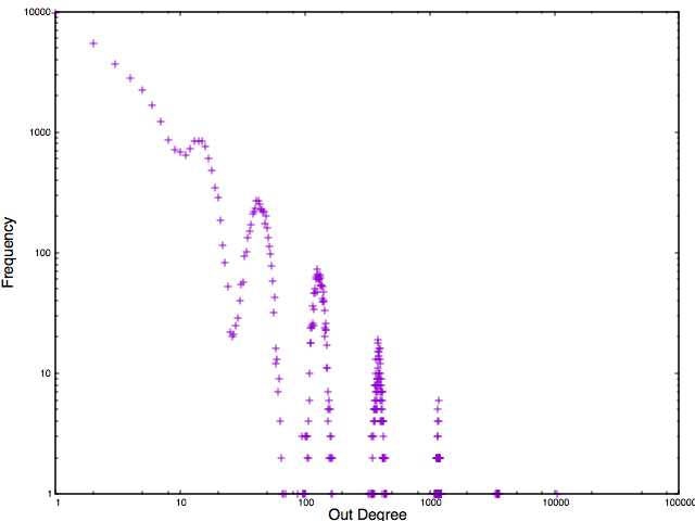
(a) ${\tt RPSKG}~{}(2^{20},0,16,T)$

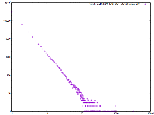
(b) ${\tt RPSKG}~{}(2^{20},1,15,T)$

Figure 3: Difference in degree distribution when only $3\times 3$ seeds are used versus when only one $2\times 2$ seed is used with multiple $3\times 3$ seeds

In this section, we discuss some of the experiments we performed. We focus on comparing some of the graphs generated by the SKG model to those generated by the RPSKG model. Note that when $k=0$, Algorithm 2 is equivalent to the SKG model — when the $3\times 3$ seed is not used in any iteration of the edge generation.

For our experiments, we applied Algorithm 3 to the Graph500 seed (see Equation 1) to obtain the following $3\times 3$ seed (approximated to 4 decimal places):

$$M=\begin{bmatrix}0.4793&0.1598&0.0533\\ 0.1598&0.0533&0.0178\\ 0.0533&0.0178&0.0059\\ \end{bmatrix}$$

We note that users can sample a $3\times 3$ seed from the uniform distribution over an arbitrary $2\times 2$ seed. The procedure for producing the seed above is thus flexible enough to accommodate additional graph characteristics.

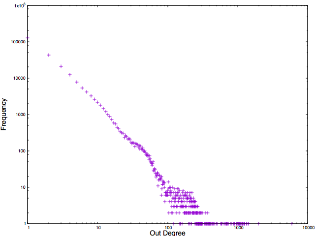
(a) ${\tt RPSKG}~{}(2^{20},9,7,T)$

(b) ${\tt RPSKG}~{}(2^{20},8,8,T)$

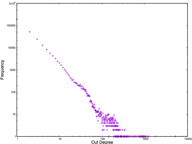
(c) ${\tt RPSKG}~{}(2^{20},7,9,T)$

Figure 4: Kinks in degree distribution observed when number of $3\times 3$ seeds used are close to number of $2\times 2$ seeds. $T$ is the $2\times 2$ Graph500 initiator seed matrix given in Equation 1.

(a) ${\tt RPSKG}~{}(2^{20},1,15,T)$

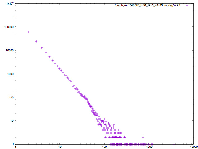
(b) ${\tt RPSKG}~{}(2^{20},3,13,T)$

Figure 5: Smaller Kinks in degree distribution observed when the number of $3\times 3$ seeds used are not as close to number of $2\times 2$ seeds.

Figures 2(a) and 2(b) illustrate the stark difference in the degree distributions of graphs generated by RPSKG and SKG models. Both plots are on a log-log scale and show the frequency of nodes in the graph for each possible (out-)degree — in essence, the degree distribution.

Figure 2(a) is a plot of the degree distribution of a graph generated by the SKG model. On the other hand, Figure 2(b) is a plot of the degree distribution when the RPSKG model is used. Both models generate the same number of edges ($2^{20}$ edges) but differ in the number of vertices generated. For the SKG model, $2^{16}$ nodes are generated but for the RPSKG model, $3\cdot 2^{15}$ nodes are generated.

As expected, Figure 2(a) shows unwanted oscillations, which according to Seshadhri et al.  [41] is most accurately characterized as fluctuating between a log-normal distribution and exponential tail.

On the other hand, using a single $3\times 3$ seed in RPSKG produces the graph shown in Figure 2(b) with no salient oscillations. This degree distribution plot seems to approximate a log-normal distribution. In essence, it appears that we are able to achieve the same objective (in terms of the generated degree distribution) as NSKG without generating or storing $\ell$ random numbers (needed for the edge generation process of Noisy SKG).

Analogously, Figures 3(a) and 3(b) illustrate the stark difference in the degree distributions of graphs generated by RPSKG and SKG models but when $3\times 3$ seeds are the primary seeds applied (as opposed to the $2\times 2$ seeds).

Figures 3(a) and 2(a) are almost indistinguishable, showing that the use of only $2\times 2$ seeds or only $3\times 3$ seeds will lead to unwanted oscillations in the degree distribution. Similar to Figure 3(b), Figure 2(b) shows the degree distribution when only one $2\times 2$ seed is applied amidst $3\times 3$ seeds. The degree distribution obtained in this figure is approximately lognormal.

Furthermore, in our experiments on the graph with $2^{20}$ edges we used $k=1\ldots 16$ $3\times 3$ seeds while keeping the total number of seeds used constant. In essence, we ran ${\tt RPSKG}~{}(2^{20},16-k,k,T)$ for $k=1\ldots 16$ where $T$ is the $2\times 2$ Graph500 initiator seed matrix (Equation 1). We noticed that the degree distributions of generated graphs look more log-normal when only a few number of either $2\times 2$ seeds or $3\times 3$ seed are used — when either $k$ or $\ell$ is close to 1.

On the other hand, we noticed that when $k$ is close to $\ell$, a kink starts to appear in the degree distribution of the generated graph. Figures  4(a), 4(b), and  4(c) show degree distributions for graphs generated with $k=7,8,$ and $9$ respectively. These three plots show a slight kink in the degree distribution. Obviously, these degree distributions do not exhibit the unwanted oscillations generated by SKG (see Figure 2(a)) but looks less log-normal than the degree distribution in Figure 2(b).

6 Conclusion

Graph models can be used to model biological networks, social networks, communication networks, relationships between products and advertisers, collaboration networks, and even the world wide web. However, major companies cannot share all of their graph data because of copyright, legal, and privacy issues. This has led to the development of graph generation algorithms, one of which is the family of stochastic kronecker graph algorithms.

We have presented criteria for statistical and computational identifiability of Stochastic Kronecker Graphs. The criteria is used to conjecture that we can classify SKG models into different classes and show implications of such conjectures. Furthermore, we also provide evidence for the conjectures via simulations. The ${\tt RPSKG}~{}$ algorithm is also presented and can be used to interpolate between the use of $2\times 2$ seeds and $3\times 3$ seeds when generating graphs via stochastic Kronecker multiplication. This algorithm can result in the removal of oscillations in the resulting degree oscillations, thus providing a superior case for its use.

We believe that our work represents a starting point for further understanding of graph generation algorithms and their properties via a systematic notion of identifiability. Furthermore, here are adjacent areas for exploration:

Separation Results

We have been able to show separation of SKG models via the statistical and computational identifiability notions. We studied two prominent properties of graphs: the existence of isolated vertices and the whether the graph is connected. However, we believe other properties could also show (parameterized) separation across SKG models and leave such exploration to future work. Definition 4 defines a Kronecker graph distribution function over any starting seed. We have defined efficient procedures for sampling seeds from another seed of relative prime dimension. It is clear that every graph has a Kronecker graph distribution but it is not immediate, under what conditions, every distribution has a corresponding realizable graph. We leave this question to future exploration.

Privacy

One of the main applications of the stochastic kronecker graph model is to generate synthetic graph data. This is also a solution to “machine unlearning” now mandated in some some regulations. The process and quality of synthetic data is a major open problem in privacy-preserving statistics and machine learning. We have identified criteria (via the identifiability notions) to measure the utility of generated graphs. However, what are the necessary conditions (e.g., on graph size) to generate graphs that are always within a given statistical distance?

Redistricting

Recent work (e.g.,  [33]) has shown random sampling of graph partitions is a popular tool for evaluating the effectiveness or bias of legislative redistricting plans. Stochastic Kronecker Graphs, with accuracy measures and effective degree distribution characteristics, can be used to evaluate similar redistricting plans from the same starting seed. We leave the applications of stochastic kronecker graphs for redistricting to future exploration.

References

- AB [06] S. Arora and B. Barak. Computational Complexity: A Modern Approach. Cambridge University Press, 2006.
- Abb [17] Emmanuel Abbe. Community detection and stochastic block models: Recent developments. J. Mach. Learn. Res., 18:177:1–177:86, 2017.
- Abb [18] Emmanuel Abbe. Community detection and stochastic block models. Found. Trends Commun. Inf. Theory, 14(1-2):1–162, 2018.
- AS [15] Emmanuel Abbe and Colin Sandon. Community detection in general stochastic block models: Fundamental limits and efficient algorithms for recovery. In Venkatesan Guruswami, editor, IEEE 56th Annual Symposium on Foundations of Computer Science, FOCS 2015, Berkeley, CA, USA, 17-20 October, 2015, pages 670–688. IEEE Computer Society, 2015.
- BBN [19] Matthew Brennan, Guy Bresler, and Dheeraj M. Nagaraj. Phase transitions for detecting latent geometry in random graphs. Probability Theory and Related Fields, 178:1215 – 1289, 2019.
- BCL [11] Peter J. Bickel, Aiyou Chen, and Elizaveta Levina. The method of moments and degree distributions for network models. The Annals of Statistics, 39(5):2280 – 2301, 2011.
- Cay [09] Arthur Cayley. A theorem on trees, volume 13 of Cambridge Library Collection - Mathematics, page 26–28. Cambridge University Press, 2009.
- CF [06] Deepayan Chakrabarti and Christos Faloutsos. Graph mining: Laws, generators, and algorithms. ACM Comput. Surv., 38(1):2, 2006.
- CF [19] Raj Chetty and John N. Friedman. A practical method to reduce privacy loss when disclosing statistics based on small samples. American Economic Review Papers and Proceedings, 109:414–420, 2019.
- CHK+ [07] Shai Carmi, Shlomo Havlin, Scott Kirkpatrick, Yuval Shavitt, and Eran Shir. A model of internet topology using ¡i¿k¡/i¿-shell decomposition. Proceedings of the National Academy of Sciences, 104(27):11150–11154, 2007.
- CJK+ [22] Raj Chetty, Matthew Jackson, Theresa Kuchler, Johannes Stroebel, Nathaniel Hendren, Robert Fluegge, Sara Gong, Federico Gonzalez, Armelle Grondin, Matthew Jacob, Drew Johnston, Martin Koenen, Eduardo Laguna-Muggenburg, Florian Mudekereza, Tom Rutter, Nicolaj Thor, Wilbur Townsend, Ruby Zhang, Mike Bailey, and Nils Wernerfelt. Social capital i: measurement and associations with economic mobility. Nature, 608:1–14, 08 2022.
- CL [02] Fan Chung and Linyuan Lu. The average distances in random graphs with given expected degrees. Proceedings of the National Academy of Sciences, 99(25):15879–15882, 2002.
- [13] Graph500 Steering Committee. Graph 500 benchmark. http://www.graph500.org/. Accessed: 2016-11-30.
- CSN [09] Aaron Clauset, Cosma Rohilla Shalizi, and Mark E. J. Newman. Power-law distributions in empirical data. SIAM Rev., 51(4):661–703, 2009.
- CZF [04] Deepayan Chakrabarti, Yiping Zhan, and Christos Faloutsos. R-MAT: A recursive model for graph mining. In Proceedings of the Fourth SIAM International Conference on Data Mining, Lake Buena Vista, Florida, USA, April 22-24, 2004, pages 442–446. SIAM, 2004.
- DWXY [20] Jian Ding, Yihong Wu, Jiaming Xu, and Dana Yang. Consistent recovery threshold of hidden nearest neighbor graphs. In Conference on Learning Theory, COLT 2020, 9-12 July 2020, Virtual Event [Graz, Austria], volume 125 of Proceedings of Machine Learning Research, pages 1540–1553. PMLR, 2020.
- DWXY [21] Jian Ding, Yihong Wu, Jiaming Xu, and Dana Yang. Consistent recovery threshold of hidden nearest neighbor graphs. IEEE Trans. Inf. Theory, 67(8):5211–5229, 2021.
- ER [60] P. Erdős and A Rényi. On the evolution of random graphs. In Publication of the Mathematical Institute of the Hungarian Academy of Sciences, pages 17–61, 1960.
- Gil [59] E. N. Gilbert. Random graphs. The Annals of Mathematical Statistics, 30(4):1141–1144, 1959.
- GM [82] Shafi Goldwasser and Silvio Micali. Probabilistic encryption and how to play mental poker keeping secret all partial information. In Proceedings of the Fourteenth Annual ACM Symposium on Theory of Computing, STOC ’82, page 365–377, New York, NY, USA, 1982. Association for Computing Machinery.
- GM [84] Shafi Goldwasser and Silvio Micali. Probabilistic encryption. Journal of Computer and System Sciences, 28(2):270–299, 1984.
- Gol [00] Oded Goldreich. Foundations of Cryptography: Basic Tools. Cambridge University Press, USA, 2000.
- Gol [04] Oded Goldreich. Pseudorandomness - part I. In Steven Rudich and Avi Wigderson, editors, Computational Complexity Theory, volume 10 of IAS / Park City mathematics series, pages 253–285. AMS Chelsea Publishing, 2004.
- GSP [11] C. Groër, B. D. Sullivan, and S. Poole. A mathematical analysis of the r-mat random graph generator. Networks, 58(3):159–170, 2011.
- Kee [10] R.W. Keener. Theoretical Statistics: Topics for a Core Course. Springer Texts in Statistics. Springer New York, 2010.
- KL [12] Myunghwan Kim and Jure Leskovec. Multiplicative attribute graph model of real-world networks. Internet Math., 8(1-2):113–160, 2012.
- KMKK [15] Mihyun Kang, Tamas Makai, Christoph Jörg Koch, and Michal Karonski. Properties of stochastic kronecker graphs. Journal of Combinatorics, 6:395–432, 2015.
- KNT [06] Ravi Kumar, Jasmine Novak, and Andrew Tomkins. Structure and evolution of online social networks. In Tina Eliassi-Rad, Lyle H. Ungar, Mark Craven, and Dimitrios Gunopulos, editors, Proceedings of the Twelfth ACM SIGKDD International Conference on Knowledge Discovery and Data Mining, Philadelphia, PA, USA, August 20-23, 2006, pages 611–617. ACM, 2006.
- KPP+ [14] Tamara G. Kolda, Ali Pinar, Todd Plantenga, C. Seshadhri, and Christine Task. Counting triangles in massive graphs with MapReduce. SIAM Journal on Scientific Computing, 36(5):S44–S77, October 2014.
- LCK+ [10] Jure Leskovec, Deepayan Chakrabarti, Jon Kleinberg, Christos Faloutsos, and Zoubin Ghahramani. Kronecker graphs: An approach to modeling networks. J. Mach. Learn. Res., 11:985–1042, March 2010.
- LCKF [05] Jure Leskovec, Deepayan Chakrabarti, Jon M. Kleinberg, and Christos Faloutsos. Realistic, mathematically tractable graph generation and evolution, using kronecker multiplication. In Alípio Jorge, Luís Torgo, Pavel Brazdil, Rui Camacho, and João Gama, editors, Knowledge Discovery in Databases: PKDD 2005, 9th European Conference on Principles and Practice of Knowledge Discovery in Databases, Porto, Portugal, October 3-7, 2005, Proceedings, volume 3721 of Lecture Notes in Computer Science, pages 133–145. Springer, 2005.
- Mar [17] Daniel Wyatt Margo. Sorting Shapes the Performance of Graph-Structured Systems. PhD thesis, Harvard University, 2017.
- MI [23] Cory McCartan and Kosuke Imai. Sequential monte carlo for sampling balanced and compact redistricting plans. Annals of Applied Statistics, Forthcoming, 2023.
- Mit [03] Michael Mitzenmacher. A brief history of generative models for power law and lognormal distributions. Internet Mathematics, 1:226–251, 2003.
- Mit [05] Michael Mitzenmacher. Editorial: The future of power law research. Internet Mathematics, 2(4):525–534, 2005.
- MNK [18] Sebastián Moreno, Jennifer Neville, and Sergey Kirshner. Tied kronecker product graph models to capture variance in network populations. ACM Trans. Knowl. Discov. Data, 12(3):35:1–35:40, 2018.
- MX [07] Mohammad Mahdian and Ying Xu. Stochastic kronecker graphs. In Algorithms and Models for the Web-Graph, 5th International Workshop, WAW 2007, San Diego, CA, USA, December 11-12, 2007, Proceedings, pages 179–186, 2007.
- New [05] M. E. J. Newman. Power laws, pareto distributions and zipf’s law. CONTEMPORARY PHYSICS, 2005.
- NS [08] Arvind Narayanan and Vitaly Shmatikov. Robust de-anonymization of large sparse datasets. In 2008 IEEE Symposium on Security and Privacy (S&P 2008), 18-21 May 2008, Oakland, California, USA, pages 111–125. IEEE Computer Society, 2008.
- SPK [12] C. Seshadhri, Ali Pinar, and Tamara G. Kolda. The similarity between stochastic kronecker and chung-lu graph models. In Proceedings of the Twelfth SIAM International Conference on Data Mining, Anaheim, California, USA, April 26-28, 2012, pages 1071–1082. SIAM / Omnipress, 2012.
- SPK [13] C. Seshadhri, Ali Pinar, and Tamara G. Kolda. An in-depth analysis of stochastic kronecker graphs. J. ACM, 60(2):13:1–13:32, May 2013.