SCoRe: Submodular Combinatorial Representation Learning for Real-World Class-Imbalanced Settings

Abstract

Representation Learning in real-world class-imbalanced settings has emerged as a challenging task in the evolution of deep learning. Lack of diversity in visual and structural features for rare classes restricts modern neural networks to learn discriminative feature clusters. This manifests in the form of large inter-class bias between rare object classes and elevated intra-class variance among abundant classes in the dataset. Although deep metric learning approaches have shown promise in this domain, significant improvements need to be made to overcome the challenges associated with class-imbalance in mission critical tasks like autonomous navigation and medical diagnostics. Set-based combinatorial functions like Submodular Information Measures exhibit properties that allow them to simultaneously model diversity and cooperation among feature clusters. In this paper, we introduce the SCoRe (Submodular Combinatorial Representation Learning) framework and propose a family of Submodular Combinatorial Loss functions to overcome these pitfalls in contrastive learning. We also show that existing contrastive learning approaches are either submodular or can be re-formulated to create their submodular counterparts. We conduct experiments on the newly introduced family of combinatorial objectives on two image classification benchmarks - pathologically imbalanced CIFAR-10, subsets of MedMNIST and a real-world road object detection benchmark - India Driving Dataset (IDD). Our experiments clearly show that the newly introduced objectives like Facility Location, Graph-Cut and Log Determinant outperform state-of-the-art metric learners by up to 7.6% for the imbalanced classification tasks and up to 19.4% for object detection tasks.

Keywords Representation Learning  $\cdot$ Submodular Functions  $\cdot$ Contrastive Learning

1 Introduction

Deep Learning models [1, 2, 3] for representation learning tasks distinguish between object classes by learning discriminative feature embeddings for each class in the training dataset. Most State-of-the-Art (SoTA) approaches adopt Cross-Entropy (CE) [4] loss as the objective function to train models on cannonical benchmarks. In contrast to curated cannonical benchmarks which present a balanced data distribution, real-world, safety critical tasks like autonomous navigation, health-care etc. demonstrate class-imbalanced settings. This introduces large inter-class bias and intra-class variance [5] between object classes while training a deep learning model which CE loss is unable to overcome.

Recent developments in this field have observed an increase in the adoption of deep metric learning approaches [6, 7, 8] and contrastive learning [9, 10, 11] strategies. In both supervised [11, 6] and unsupervised [12] learning settings, these techniques operate on image pairs, rewarding pairs with the same class label ($positive$) to be closer while pairs from different class labels ($negative$) to be farther away in the feature space. Unfortunately, these approaches use pairwise metrics in their objectives which cannot guarantee the formation of tight or disjoint feature clusters in real-world settings. The experiments conducted by us in this paper show that the aforementioned pitfalls lead to poorer performance of these techniques in real-world, class-imbalanced settings. This requires us to study metric learners from a combinatorial point of view by considering class specific feature vectors as sets and employing objectives that jointly model inter-class separation and intra-class compactness. Generalization of set-based information-theoretic functions like entropy, facility-location etc., also known as submodular functions [13] have been shown [14] to be effective in modeling diversity, representation, coverage, and relevance among sets in various machine learning tasks like active learning [15, 16] and subset selection [17, 18].

Figure 1: The effect of class-imbalance on the performance metrics ($mAP_{50}$) for the object detection task of the India Driving Dataset (IDD). As the class frequency (shown as blue line) decreases, proposed objectives in SCoRe (shown in red) consistently outperforms SoTA approaches like SupCon (shown in green) in detecting rare road objects like bicycle, traffic light etc. in IDD.

In this paper, we propose a framework - Submodular Combinatorial Representation Learning (SCoRe) - that introduces set-based submodular combinatorial loss functions to overcome the challenges in class-imbalanced settings as shown in Figure 1. We propose a family of objective functions based on popular submodular functions [19] such as Graph-Cut, Facility Location and Log-Determinant. These set-based loss functions maximize the mutual information [20] between class-specific sets while preserving the most discriminative features for each set (class) thereby reducing the effect of inter-class bias and intra-class variance. Our results in Section 4 show that our proposed loss functions consistently outperform SoTA approaches in metric learning for class-imbalanced classification tasks for CIFAR-10 and MedMNIST [21] datasets alongside object detection in real-world unconstrained traffic environments like in India Driving Dataset (IDD) [22]. The main contributions of this paper can be summarized below:

• We introduce a novel submodular combinatorial framework of loss functions (SCoRe) which demonstrates resilience against class-imbalance for representation learning while outperforming SoTA approaches by up to 7.6% for classification task and 19.4% for object detection tasks.

• We highlight that existing contrastive learning objectives are either submodular or can be reformulated as submodular functions. We show that the submodular counterparts of these contrastive losses outperform their non-submodular counterparts by 3.5 - 4.1%.

• Finally, we demonstrate the performance of our proposed objectives for road object detection in real-world class-imbalanced setting like in [22] and show improvements up to 19.4% proving the reliability of our approach in real-world downstream tasks.

2 Related Work

Deep Metric Learning:

Traditional deep-learning approaches have been trained using Cross-Entropy (CE) [23, 4] loss in the supervised setting. It has shown great success on cannonical benchmarks by maximizing the log likelihood of a data point to be of its corresponding ground-truth label. Unfortunately, models trained using this objective are not robust to class-imbalance, noisy labels etc. Recent approaches in supervised learning adopt metric learning [7, 8, 6, 24] which learns a distance [9] or a similarity [7, 8] metric to enforce orthogonality in the feature space [6] while learning discriminative class-specific features. Approaches like [8, 25] adopt similarity metrics like cosine-similarity [8] to align feature vectors belonging to the same class along their cluster centroids while maintaining orthogonality among cluster centroids from diverse classes. To ensure a minimum margin between the feature clusters in tasks like face recognition, [7] a margin has been applied in the objective function. Unfortunately, these approaches are unable to ensure formation of compact feature clusters for each class and formation of disjoint clusters as they operate on pairwise similarity metrics between instances and not on the complete set of instances in a class.

Contrastive Learning:

Another branch in representation learning, also known as contrastive learning, stems from noise contrastive estimation [26] and is popular in self-supervised learning [12, 27, 28] where no label information is available during model training. Unlike mining for positive and negative pairs, these techniques use augmented samples [12] as positive examples while other samples in the batch are considered negative examples. This objective has also been applied in the supervised setting in SupCon [11]. Unlike existing approaches in metric learning [9, 10] , these approaches aim to learn discriminative feature clusters rather than aligning features to their cluster centroids. SupCon differs from existing metric learners by the number of positive and negative pairs used in the loss function. Triplet loss [9] uses only 1 positive pair and 1 negative pair. N-pairs [10] loss contrasts only 1 positive pair against multiple negative pairs while SupCon contrasts between multiple positive and negative pairs. Lifted-Structure loss [29] contrasts the similarity between positive image pairs and hardest negative pair. Additionally, SupCon bears close resemblance to Soft-Nearest Neighbors loss [30] and maximizes the entanglements (relative position of positive pairs with respect to negative pairs) between classes. Although, these methods have demonstrated great success, they continue to adopt pairwise similarity metrics and are thus cannot guarantee formation of disjoint clusters. From our experiments in Section 4 , we also show that SoTA metric learners are unable to overcome inter-class bias and intra-class variance and continue to plague representation learning tasks particularly in real-world class-imbalanced settings.

Submodular Functions:

Submodular functions are set functions that satisfy a natural diminishing returns property. A set function $f:2^{V}\rightarrow\mathbb{R}$ (on a ground-set $V$) is submodular if it satisfies $f(X)+f(Y)\geq f(X\cup Y)+f(X\cap Y),\forall X,Y\subseteq V$ [31]. These functions have been studied extensively in the context of data subset selection [20] , active learning [15] and video-summarization [14, 20]. Submodular functions are capable of modelling diversity, relevance, set-cover etc. which allows them to discriminate between different classes or slices of data while ensuring the preservation of most relevant features in each set. Very recent developments in the field have applied submodular functions like Facility-Location in metric learning [32]. These properties of submodular functions can be used to learn diverse feature clusters in representation learning tasks which is a field yet to be studied in literature.

To the best of our knowledge , we are the first to demonstrate that combinatorial objectives using submodular functions are superior in creating tighter and well-separated feature clusters for representation learning. We are fore-runners in showing through Section 4 that most of the existing contrastive learning approaches have a submodular variant which have shown to outperform their non-submodular counterparts.

3 Method

Figure 2: Overview of Combinatorial Objectives in SCoRe with respect to contrastive and metric learners.

In this section we describe the various components of our framework - SCoRe , for supervised representation learning tasks. Our framework is structurally similar to [11] and [12] with modifications to contrast existing metric learning approaches against submodular combinatorial objectives.

3.1 SCoRe: Submodular Combinatorial Representation Learning Framework

Supervised training for representation learning tasks proceed with learning a feature extractor $f(I,\theta)$ followed by a classifier $Clf(f(I,\theta))$ which categorizes an input image $I$ into its corresponding class label $c_{i}$, where $c_{i}\in[1,2,...C]$. Unlike standard model training for image classification , our supervised learning framework consists of three major components and is trained using a two-stage training strategy as introduced in [11] : (1) Feature Extractor , $f(I,\theta)$ is a convolutional neural network [1, 3, 2] which projects an input image $I$ into a $D_{f}$ dimensional feature space $r$, where $r=f(I,\theta)\in\mathbb{R}^{D_{f}}$, given parameters $\theta$. In this paper we adopt residual networks [2] (specifically ResNet-50) as our feature extractor and aim to learn its parameters $\theta$ using an objective function described below. (2) Classifier , $Clf(r,\theta)$ is a linear projection layer that projects the $D_{f}$ dimensional input features $r$ to a smaller $D_{p}$ dimensional vector $z$, where $z=Clf(r,\theta)\in\mathbb{R}^{D_{p}}$ such that a linear classifier can classify the input image $I$ to its corresponding class label $c_{i}$ for $i\in[1,C]$. (3) Combintorial Loss Functions , $L(\theta)$ trains the feature extractor $f$ over all classes $C$ in the dataset to discriminate between classes in a multi-class classification setting. Contrastive and combinatorial losses largely depend on feature distance $D_{ij}(\theta)$ or similarity $S{ij}(\theta)$ between pairs/sets $i$ and $j$ to compute the loss metric which depends on $\theta$. By varying the objective function for a given metric , we are able to study their behavior in learning discriminative feature sets for each class in $\mathcal{T}$.

Training and evaluation of models using this proposed framework occurs in two stages. In stage 1 we train a generalizable feature extractor $f(I,\theta)$ using multiple variants of $L(\theta)$ on a large scale image dataset $\mathcal{T}$ containing ${x_{i},y_{i}}_{i=1,2,...|\mathcal{T}|}$. In stage 2, we freeze the feature extractor $f(I,\theta)$ and train only a linear classifier $Clf(r,\theta)$ on the embeddings ($r$) generated by the feature extractor, using the standard cross-entropy loss [23]. Using this framework we also propose a novel family of combinatorial objective functions which is formulated as the sum of submodular functions [19] and is discussed in Section 3.2.

Table 1: Summary of various objective functions studied through SCoRe framework and their respective combinatorial properties (detailed derivations in section A.5 of the appendix).

Objective Function	Equation $L(\theta,A_{k})$	Combinatorial
		Property
Triplet Loss [9]	$L(\theta,A_{k})=\sum_{\begin{subarray}{c}i,p\in A_{k},\\ n\in\mathcal{V}\setminus A_{k}\end{subarray}}max(0,D_{ip}^{2}(\theta)-D_{in}^{2}(\theta)+\epsilon)$	Not Submodular
N-Pairs Loss [10]	$L(\theta,A_{k})=-[\sum_{i,j\in A_{k}}S_{ij}(\theta)+\sum_{i\in A_{k}}log(\sum_{j\in\mathcal{V}}S_{ij}(\theta)-1)]$	Submodular
OPL [6]	$L(\theta,A_{k})=(1-\sum_{i,j\in A_{k}}S_{ij}(\theta))+(\sum_{i\in A_{k}}\sum_{j\in\mathcal{V}\setminus A_{k}}S_{ij}(\theta))$	Submodular
SNN [30]	$L(\theta,A_{k})=-\sum_{i\in A_{k}}[\log\sum_{j\in A_{k}}\exp(S_{ij}(\theta))-\log\sum_{j\in\mathcal{V}\setminus A_{k}}\exp(S_{ij}(\theta))]$	Not Submodular
SupCon [11]	$L(\theta,A_{k})=[\frac{-1}{|A_{k}|}\sum_{i,j\in A_{k}}S_{ij}(\theta)]+\sum_{i\in A_{k}}[log(\sum_{j\in\mathcal{V}}S_{ij}(\theta)-1)]$	Not Submodular
Submod-Triplet	$L(\theta,A_{k})=\sum_{\begin{subarray}{c}i\in A_{k}\\ n\in\mathcal{V}\setminus A_{k}\end{subarray}}S_{in}^{2}(\theta)-\sum_{i,p\in A}S_{ip}^{2}(\theta)$	Submodular
Submod-SNN	$L(\theta,A_{k})=\sum_{i\in A_{k}}[\log\sum_{j\in A_{k}}\exp(D_{ij}(\theta))+\log\sum_{j\in\mathcal{V}\setminus A_{k}}\exp(S_{ij}(\theta))]$	Submodular
Submod-SupCon	$L(\theta,A_{k})=-[\sum_{i,j\in A_{k}}S_{ij}(\theta)]+\sum_{i\in A_{k}}[log(\sum_{j\in\mathcal{V}\setminus A_{k}}\exp(S_{ij}(\theta)))]$	Submodular
Graph-Cut [$S_{f}$] (ours)	$L(\theta,A_{k})=\sum_{i\in A_{i}}\sum_{j\in\mathcal{V}\setminus A_{k}}S_{ij}(\theta)-\lambda\sum_{i,j\in A_{k}}S_{ij}(\theta)$	Submodular
Graph-Cut [$C_{f}$] (ours)	$L_{C_{f}}(\theta,A_{k})=\lambda\sum_{i\in A_{i}}\sum_{j\in\mathcal{V}\setminus A_{k}}S_{ij}(\theta)$	Submodular
Log-Determinant [$S_{f}$] (ours)	$L(\theta,A_{k})=\log\det(S_{A_{k}}(\theta)+\lambda\mathbb{I}_{|A_{k}|})$	Submodular
Log-Determinant [$C_{f}$] (ours)	$L(\theta,A_{k})=\log\det(S_{A_{k}}(\theta)+\lambda\mathbb{I}_{|A_{k}|})-\log\det(S_{\mathcal{V}}(\theta)+\lambda\mathbb{I}_{|\mathcal{V}|})$	Submodular
Facility-Location [$C_{f}$/ $S_{f}$] (ours)	$L(\theta,A_{k})=\sum_{i\in\mathcal{V}\setminus A_{k}}max_{j\in A_{k}}S_{ij}(\theta)$	Submodular

3.2 Combinatorial Loss Functions

As introduced in Section 3.1 we propose a set of combinatorial loss functions which promotes the learning of tighter and well-separated feature clusters in the embedding space. This family of objectives considers each class $c_{k}$ in the dataset $\mathcal{T}$ as a set $A_{k}$ where $k\in[1,C]$. The task of $f$ is to learn the model parameters $\theta$ using $L(\theta)$ to enforce sufficient decision boundaries between the feature clusters while rewarding the formation of tighter clusters for each class $A_{k}$. The overall loss $L(\theta)$ can be defined as the sum over the loss $L(\theta,A_{k})$ calculated for each set $A_{k}$ in the dataset, $L(\theta)=\sum_{k=1}^{|C|}L(\theta,A_{k})$. Given multiple sets ${A_{1},A_{2},A_{3},....A_{|C|}}$ (each set contains instances of a single class) and a ground set $\mathcal{V}$ (which is the entire dataset), and a submodular function $f$, different formulations of combinatorial information measures [31] can be defined. Define the Total Submodular Information as: $S_{f}(A_{1},A_{2},A_{3},\dots,A_{|C|})=\overset{|C|}{\underset{k=1}{\sum}}f(A_{k})$. Also, we can define the Total Submodular Correlation as: $C_{f}(A_{1},A_{2},A_{3},\dots,A_{|C|})=\sum_{k=1}^{|C|}f(A_{k})-f(\overset{|C|}{\underset{k=1}{\cup}}A_{k})$. Given any submodular function, we can define two variants of combinatorial loss functions:

$$L_{S_{f}}(\theta)=S_{f}(A_{1},\cdots,A_{|C|}),\,\,\,L_{C_{f}}(\theta)=C_{f}(A_{1},\cdots,A_{|C|})$$ (1)

The functions that we consider in this work, are defined with similarity kernels $S$, which in turn depend on the parameters $\theta$. A loss function which minimizes $S_{f}$ maximizes the intra-cluster similarity (by minimizing the submodular function on each cluster), while the loss function that minimizes $C_{f}$ trades-off between maximizing the intra-cluster similarity but also minimizes the inter-cluster similarity (by maximizing $f(\cup_{k}A_{k})$).We select the best of these information-theoretic formulations effectively in our framework to design a family of objective functions as shown in Table 1 for representation learning tasks.

3.2.1 SCoRe: Submodular Combinatorial Loss Functions

In this paper we propose three novel objective functions based on submodular information measures : Facility-Location (FL), Graph-Cut (GC), and Log Determinant (LogDet) as $L(\theta,A_{k})$ and minimize them to overcome inter-class bias and intra-class variance. We adopt the cosine similarity metric $S_{ij}(\theta)$ as used in SupCon [11] which can be defined as $S_{ij}(\theta)=f(I_{i},\theta)^{\text{T}}\cdot f(I_{j},\theta)/||f(I_{i},\theta)||\cdot||f(I_{j},\theta)||$. For objective functions which adopt a distance metric $D_{ij}$ we adopt the euclidean distance as in [9].

Facility Location (FL) based objective function minimizes the maximum similarity $S$ between sets of features belonging to different classes, $S_{ij}$ where $i\neq j$. The equation describing this objective is shown in Equation 2. This objective function ensures that the the sets $A_{k}\in\mathcal{V}$ are disjoint by minimizing the similarity between features in $A_{k}$ and the hardest negative feature vectors in $\mathcal{V}\setminus A_{k}$. Inherently, this function also learns the cluster centroid [31, 19] for each $A_{k}$ in the embedding space thus proving to be effective in overcoming inter-cluster bias in downstream tasks.

$$L_{S_{f}}(\theta,A_{k})=\sum_{i\in\mathcal{V}\backslash A_{k}}max_{j\in A_{k}}S_{ij}(\theta)+|\mathcal{V}|,\,\,\,L_{C_{f}}(\theta,A_{k})=\sum_{i\in\mathcal{V}\backslash A_{k}}max_{j\in A_{k}}S_{ij}(\theta)$$ (2)

Note that in the case of FL, $L_{S_{f}}$ and $L_{C_{f}}$ differ by a constant, and are the same loss. We also point out that this loss function naturally handles the cases where the classes are imbalanced: it boosts the imbalanced classes since $\mathcal{V}\backslash A_{k}$ is actually going to be larger for imbalanced classes compared to the more frequent classes. As expected, the FL loss performs the best in imbalanced data settings.

Graph Cut (GC) based representation learning function described in Equation 3 minimizes the pairwise similarity between feature vectors between a positive set $A_{k}$ and the remaining negative sets in $\mathcal{V}\setminus A_{k}$ while maximizing the similarity between features in each set $A_{k}$. This objective bears the closest similarity to existing contrastive learners that adopt pairwise similarity metrics (refer Section 3.2.2) and jointly models inter-cluster separation and intra-cluster compactness which are effective in overcoming class-imbalance in representation learning. Specifically, the Orthagonal Projection Loss (OPL) and a version of Triplet Loss are special cases of of the GC based loss function.

$$L_{S_{f}}(\theta,A_{k})=\sum_{i\in A_{i}}\sum_{j\in\mathcal{V}\setminus A_{k}}S_{ij}(\theta)-\lambda\sum_{i,j\in A_{k}}S_{ij}(\theta),\,\,\,L_{C_{f}}(\theta,A_{k})=\lambda\sum_{i\in A_{k}}\sum_{j\in\mathcal{V}\setminus A_{k}}S_{ij}(\theta)$$ (3)

Log-Determinant (LogDet) function measures the volume of a set $A_{k}$ in the feature space. Minimizing the LogDet over a set of datapoints in set $A_{k}$ shrinks the feature volume forming a tighter cluster. On the other hand, maximizing the LogDet over the entire ground-set $\mathcal{V}$ ensures diversity in the feature space which results in well separated feature clusters. The total correlation formulation $C_{f}$ of LogDet demonstrates the aforementioned properties which we propose as a loss function $L(\theta,A_{k})$ as shown in Equation 4. The proposed objective minimizes the LogDet over the samples in a class $A_{k}$ while maximizing the diversity in the feature space $\mathcal{V}$.

$$L_{S_{f}}(\theta,A_{k})=\log\det(S_{A_{k}}(\theta)+\lambda\mathbb{I}_{|A_{k}|}),\,\,\,L_{C_{f}}(\theta,A_{k})=L_{S_{f}}(\theta,A_{k})-\log\det(S_{\mathcal{V}}(\theta)+\lambda\mathbb{I}_{|\mathcal{V}|})$$ (4)

The $S_{f}$ version captures intra-cluster similarity, while the $C_{f}$ version (which empirically we see works better) captures both intra-cluster similarity and inter-cluster dissimilarity.

Adopting set-based information-theoretic functions $L(\theta)$ defined in SCoRe has been shown to outperform existing pairwise similarity-based loss functions. Through our experiments in Section 4 – we demonstrate that minimizing $L(\theta)$ for the functions discussed above is effective in forming compact and disjoint feature clusters in embedding space even under extreme class-imbalance scenarios. This proves the effectiveness of submodular functions in representation learning. We also show in the next section, that existing approaches in metric learning, are special cases of SCoRe.

3.2.2 SCoRe Generalizes Existing Metric/Contrastive Learning Loss Functions

In Section 2 we explore various existing approaches in metric learning and contrastive learning [11, 12] in the supervised setting. These contrastive learners mostly adopt pairwise similarity $S$ or distance $D$ metrices to learn discriminative feature sets. Interestingly, many of these existing loss functions are either special cases of SCoRe (i.e., there exist submodular functions such that the loss functions are SCoRe instantiated with those submodular functions) or closely related. We study Triplet-Loss [9], N-pairs loss [10], SupCon [11], Orthogonal Projection Loss (OPL) [6], and Soft Nearest Neighbor (SNN) [30] losses. From Table 1 we see that most contrastive learning objectives are either submodular or can be re-formulated as a submodular function. OPL and N-pairs loss are submodular, while SupCon, SNN, and Triplet losses are not naturally submodular. However, as we see in rows 7 through 9 of Table 1, we can modify these loss functions a little and we get submodular versions. We call them Submod-Triplet loss, Submod-SNN loss and Submod-SupCon loss. The proofs of submodularity for the proposed objectives are included in Section A.5 of the appendix. The experiments conducted on these functions in Section 4 show that the submodular variants of these objectives are better than the non-submodular counterparts, thus demonstrating the value of SCoRe.

4 Experiments

We conduct experiments to evaluate the proposed objective functions in the SCoRe framework against various existing objective functions in metric learning as discussed in Section 3. We perform experiments on three major settings as discussed in Section 4.1 to evaluate the effectiveness of the proposed combinatorial objectives and demonstrate their results in Sections 4.2 and 4.3.

Figure 3: Data Distribution of CIFAR-10 and MedMNIST datasets under the class-imbalanced setting. Subfigure (a) depicts the balanced setting, (b,c) depicts the pathological class imbalanced settings in CIFAR-10 and (d,e) depict the naturally imbalanced OrganAMNIST and DermaMNIST datasets respectively.Abbreviations are included in section A.1 of the appendix.

4.1 Experimental Setup

Class-Imbalanced Image Classification : We perform our experiments on two imbalanced settings of the CIFAR-10 [33] and two naturally imbalanced subsets of MedMNIST [21] datasets respectively. The results are discussed in Section 4.2. CIFAR-10 dataset consists of 10 non-overlapping classes with 6000 images per class, each of size $[32\times 32]$. In the first setting, we create a pathological longtail distribution by sampling random samples using an exponentially decaying function. In the second case, we use the hierarchy already available in the dataset to create a step based imbalanced distribution. In contrast to pathological imbalance MedMNIST dataset demonstrates natural imbalance. We conduct our experiments on the OrganAMNIST and DermaMNIST subsets of MedMNIST due to the presence of extreme imbalance in data distributions. The data distributions of the adopted benchmarks are depicted in Figure 3. The OrganAMNIST dataset consists of 1-channel $[28\times 28]$ dimensional axial slices from CT volumes, highlighting 11 distinct organ structures for a multi-class classification task. DermaMNIST presents dermatoscopic images of pigmented skin lesions, with 7 distinct dermatological conditions. Our proposed framework adopts the architecture and training strategy similar to [11]. The backbone for the feature extractor is chosen to be a ResNet-50 [2]. The stage 1 training proceeds with training the backbone on normalized 128 dimensional feature vectors using $L(\theta)$. In stage 2 we freeze the backbone and use the output of the final pooling layer to train a linear classifier $Clf$. For every objective function we report the top-1 classification accuracy after completing two stages of model training.

Table 2: Multi-class classification performance (Top1-Accuracy %)of submodular combinatorial objectives (shaded in Green) against existing approaches in metric learning and their submodular variants (shaded in blue) on Class-Imbalanced CIFAR-10 (columns 2 - 3)and MedMNIST (columns 4 - 5) datasets. We also compare the performance of these approaches in both the balanced and imbalanced settings.

Objective Function	CIFAR-10		MedMNIST
	Pathological	Pathological	OrganMNIST	DermaMNIST
	LongTail	Step	(Axial)
Cross-Entropy (CE)	86.44	74.49	81.80	71.32
Triplet Loss [9]	85.94	74.23	81.10	70.92
N-Pairs [10]	89.70	73.10	84.84	71.82
Lifted Structure Loss [29]	82.86	73.98	84.55	71.62
SNN [30]	83.65	75.97	83.85	71.87
Multi-Similarity Loss [24]	82.40	76.72	85.50	71.02
SupCon [11]	89.96	78.10	87.35	72.12
Submod-Triplet (ours)	89.20	74.36	86.03	72.35
Submod-SNN (ours)	89.28	78.76	86.21	71.77
Submod-SupCon (ours)	90.81	81.31	87.48	72.51
Graph-Cut [$S_{f}$] (ours)	89.20	76.89	86.28	69.10
Graph-Cut [$C_{f}$] (ours)	90.83	87.37	87.57	72.82
LogDet [$C_{f}$] (ours)	90.80	87.00	87.00	72.04
FL [$C_{f}$/ $S_{f}$] (ours)	91.80	87.49	87.22	73.77

Class-Imbalanced Object Detection - We also perform experiments on real-world class-imbalanced settings demonstrated by the India Driving Dataset [22] (IDD) in Section 4.3. IDD-Detection dataset demonstrates an unconstrained driving environment, characterized by natural class-imbalance, high traffic density and large variability among object classes. This results in the presence of rare classes like autorickshaw, bicycle etc. and small sized objects like traffic light, traffic sign etc. There are a total of  31k training images in IDD and  10k validation images of size $[1920\times 1080]$ with high traffic density, occlusions and varying road conditions. We adopt the detectron framework for training and evaluating the object detection model. The architecture of the object detector is a Faster-RCNN [34] model with a ResNet-101 backbone. We adopt the Feature Pyramidal Network (FPN) as in [35] to handle varying object sizes in traffic environments.

Our models are trained on 2 NVIDIA A6000 GPUs with additional details provided in Section A.2 of the appendix. Alongside experiments on benchmark datasets we conduct experiments on a synthetic dataset described in Section A.3 of the appendix section, which demonstrate the characteristics of the newly introduced loss functions in SCoRe.

Table 3: Object detection performance on India Driving Dataset (IDD). Applying our combinatorial objectives on a Faster-RCNN + FPN model produces the best Mean Average Precision ($mAP$) on real-world class-imbalanced settings.

Method	Backbone and head	$mAP$	$mAP_{50}$	$mAP_{75}$
YOLO -V3[36]	Darknet-53	11.7	26.7	8.9
Poly-YOLO [37]	SE-Darknet-53	15.2	30.4	13.7
Mask-RCNN [38]	ResNet-50	17.5	30.0	17.7
Retina-Net [35]	ResNet-50 + FPN	22.1	35.7	23.0
Faster-RCNN [34]	ResNet-101	27.7	45.4	28.2
Faster-RCNN + FPN	ResNet-101 + FPN	30.4	51.5	29.7
Faster-RCNN + SupCon	ResNet-101 + FPN	31.2	53.4	30.5
Faster-RCNN + Graph-Cut [$C_{f}$]	ResNet-101 + FPN	33.6	56.0	34.6
Faster-RCNN + Facility-Location [$S_{f}/C_{f}$]	ResNet-101 + FPN	36.3	59.5	37.1

4.2 Results on Class-Imbalanced Image Classification task

In this section , we discuss the results of training the proposed architecture in Section 4.1 on pathologically imbalanced CIFAR-10 and naturally imbalanced MedMNIST benchmarks.
CIFAR-10 : This benchmark consists of two settings - Longtail and step as described in Section 4.1. For both the imbalanced settings in CIFAR-10, we show that submodular combinatorial objective functions outperform SoTA metric learners like SupCon by upto 2% (shown by FL) for the longtail distribution and upto 7.6% (shown by FL) for the step distribution. Amongst existing contrastive learning approaches, objective functions which consider multiple positive and negative pairs (SupCon) demonstrate significant performance improvements. The reformulated submodular objectives - Submod-Triplet, Submod-SNN and Submod-SupCon demonstrate upto 3.5%, 3.7% and 4.11% respectively over their non-submodular counterparts.
MedMNIST : The natural class imbalance and the large variability in patient data demonstrated in MedMNIST serves as a playground for highlighting the effectiveness of our combinatorial objectives in overcoming class imbalance. As discussed in Section 4.1 we consider two popular subsets of the MedMNIST dataset - DermaMNIST and OrganAMNIST, the data-distribution for which has been depicted in Figure 3 (d,e). For both OrganAMNIST and DermaMNIST subsets discussed in Section 4.1, we show that proposed combinatorial objectives in SCoRe outperform SoTA approaches by upto 0.25% (as shown in GC) and 1.5% ( as shown in FL) respectively. For the OrganAMNIST dataset, the lack of variability in features (2D images) between classes leads to a smaller gain in performance, maximum being 0.25% by the Graph-Cut based objective function. Similar to CIFAR-10 benchmark we also observe that, reformulated submodular objectives of existing contrastive losses consistently outperform their non-submodular counterparts.

Results on these benchmarks, indicate the applicability of submodular combinatorial objectives in the SCoRe framework for various real-world settings by consistently outperforming SoTA approaches by significant margins.

4.3 Results on Object Detection task on Real-World Class-Imbalanced Setting

We benchmark the performance of SoTA single and two-stage object detectors against our proposed combinatorial objectives. At first, we introduce a contrastive learning based objective (SupCon) in the box classification head of the object detector and show that contrastive learning outperforms standard model training (using CE loss) on IDD by 2.16 % (0.8 $mAP$ points). Secondly, we introduce the submodular combinatorial objectives introduced in Section 3 in the box classification head and show that they outperform the SoTA as well as the contrastive learning objective [11]. The results in Table 3 show that the Facility Location and Graph-Cut based objective function outperforms the SoTA method by 19.4 % (6.1 $mAP$ points) and 16.3 % (2.6 $mAP$ points) over SupCon. Additionally, from the class-wise performance as shown in Figure 1, submodular combinatorial objectives demonstrate a sharp rise in performance ($mAP_{50}$ value) of the rare classes (a maximum of 6.4 $mAP$ points for Bicycle class) over the contrastive objective.

Figure 4: Comparison of Confusion Matrix plots between (a) SupCon [11], (b) Graph-Cut (GC), (c) Log Determinant, and (d) Facility Location (FL) for the longtail imbalanced setting of CIFAR-10 dataset. We show significant reduction in inter-class bias when employing combinatorial objectives in SCoRe characterized by reduced confusion between classes.

4.4 Does Combinatorial Loss Functions Form Better Clusters ?

As discussed in Section 3, real-world setting like MedMNIST and IDD, introduce inter-class bias and intra-class variance during model training as a resultant of class-imbalance. Confusion matrix plots on predicted class labels after stage 2 of model training are used to compare the objective functions studied in SCoRe to form disjoint clusters, therby overcoming class-imbalance. We compare between SoTA approach SupCon, and proposed GC, LogDet and FL based objective functions for the longtail imbalanced CIFAR-10 dataset. Plots in Figure 4 show that SupCon shows 2̃2% overall confusion with elevated confusion between the animal hierarchy of CIFAR-10. A significant drop in confusion is observed in combinatorial objectives with a minimum of 8.2% for FL. Both GC and LogDet demonstrate confusion between structurally similar objects like cat and dog (4-legged animals). As discussed in [39], the reduction in confusion by objectives proposed in SCoRe shows a reduction in inter-class bias. This is correlated to reducing the impact of class-imbalance due to formation of discriminative feature clusters. Thus we show that Submodular combinatorial objectives are a better choice over SoTA metric learners for representation learning tasks.

5 Conclusion

We introduce a family of submodular combinatorial objectives for representation learning tasks through the SCoRe framework to overcome class imbalance in real-world vision tasks. The proposed combinatorial objectives drive a paradigm shift in training strategy from pairwise distance or similarity matrices in SoTA approaches to set-based loss functions in SCoRe. The proposed SCoRe frameowork also highlights that existing approaches in metric/contrastive learning are either submodular in nature or can be reformulated into submodular forms. We conduct our experiments on two image classification benchmarks, namely, pathologically imbalanced CIFAR-10 and naturally imbalanced MedMNIST, alongside a real-world unconstrained object detection benchmark, namely the Indian Driving Dataset (IDD). Our proposed combinatorial loss functions outperform existing SoTA approaches on all three benchmarks by upto 7.6% for the classification task and 19.4% on the detection task. Our experiments also suggest that combinatorial counterparts of existing objectives outperform their original functions by significant margins. This establishes the importance of combinatorial loss functions in overcoming class-imbalance and its underlying pitfalls in representation learning tasks.

Appendix A Appendix

A.1 Notations

Following the problem definition in Section 3.1 we introduce several important notations in Table 4 that are used throughout the paper.

Table 4: Collection of notations used in the paper.

Symbol	Description
$\mathcal{T}$	The training Set. $|\mathcal{T}|$ denotes the size of the training set.
$\mathcal{V}$	Ground set containing feature vectors from all classes in $\mathcal{T}$.
$f(x,\theta)$	Convolutional Neural Network used as feature extractor.
$Clf(.,.)$	Multi-Layer Perceptron as classifier.
$\theta$	Parameters of the feature extractor.
$S_{ij}(\theta)$	Similarity between images $i,j\in\mathcal{T}$.
$D_{ij}(\theta)$	Distance between images $i,j\in\mathcal{T}$.
$p$	Positive sample which is of the same class $c_{i}$ as the anchor $a$.
$n$	Negative sample which is of the same class $c_{i}$ as the anchor $x$.
$A_{k}$	Target set containing feature representation from a single class $k\in c_{i}$.
$L(\theta)$	Loss value computed over all classes $c_{i}\in C$.
$L(\theta,A_{k})$	Loss value for a particular set/class $A_{k}$ given parameters $\theta$.
AK	Actinic Keratoses
BCC	Basal Cell Carcinoma
KLL	Keratosis-Like-Lesions
DF	Dermatofibroma
M	Melanoma
MN	Melanocytic Nevi
VL	Vascular Lesions

A.2 Experimental Setup : Additional Information

Class-Imbalanced Image Classification : The SCoRe framework introduces two pathological imbalance settings - Longtail and Step in the CIFAR-10 benchmark. We create the longtail distribution by sampling random samples using an exponentially decaying function. The decay rate of the function is set to $1/10$ which results in the longtail subclass to have 600 samples while the abundant subclass has 6000 samples. The step function based imbalance setting explots the hierarchy already available in the dataset. The CIFAR-10 dataset can be broadly classified into animal and automobile classes. We use this information to subsample the animal (chosen at random) class objects to create an imbalanced step data distribution. The distributions of the dataset is depicted in Figure 3. We train our models in stage 1 with a batch size of 512 (1024 after augmentations) with an initial learning rate of 0.4, trained for 1000 epochs with a cosine annealing scheduler. In stage 2 we freeze the backbone and use the output of the final pooling layer to train a linear classifier $Clf$ with a batch size of 512 and a constant learning rate of 0.8.

Class-Imbalanced Medical Image Classification : In contrast to pathological imbalance introduced in CIFAR-10 we benchmark our proposed objectives in the SCoRe framework against SoTA approaches in contrastive learning on two subsets of MedMNIST [21] dataset. The OrganAMNIST dataset consists of axial slices from CT volumes, highlighting 11 distinct organ structures for a multi-class classification task. Each image is of size $[1\times 28\times 28]$ pixels. The DermaMNIST subset presents dermatoscopic images of pigmented skin lesions, also resized to $[3\times 28\times 28]$ pixels. This dataset supports a multi-class classification task with 7 different dermatological conditions. The OrganAMNIST dataset contains 34581 training and 6491 validation samples of single channel images highlighting various modalities of 8 different organs. Although the DermaMNIST has RGB images, it is a small scale dataset with a total of 7007 training samples and 1003 validation samples. For both these subsets used in our framework, pixel values were normalized to the range $[0,1]$, and we relied on the standard train-test splits provided with the datasets for our evaluations. The results from the experiments are discussed in Section 4.2.

Class-Imbalanced Object Detection - IDD-Detection dataset demonstrates an unconstrained driving environment, characterized by natural class-imbalance, high traffic density and large variability among object classes. This results in the presence of rare classes like autorickshaw, bicycle etc. and small sized objects like traffic light, traffic sign etc. There are a total of  31k training images in IDD and  10k validation images of size $[3\times 1920\times 1080]$ with high traffic density, occlusions and varying road conditions. The architecture of the object detector is a Faster-RCNN [34] model with a ResNet-101 backbone alongside the Feature Pyramidal Network (FPN) as in [35] to handle varying object sizes in traffic environments. The model is trained for 17000 iterations with a batch size of 8 and an initial learning rate of 0.02. A step based learning rate scheduler is adopted to reduce the learning rate by 1/10 at regular intervals.

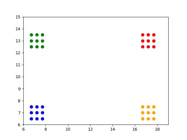
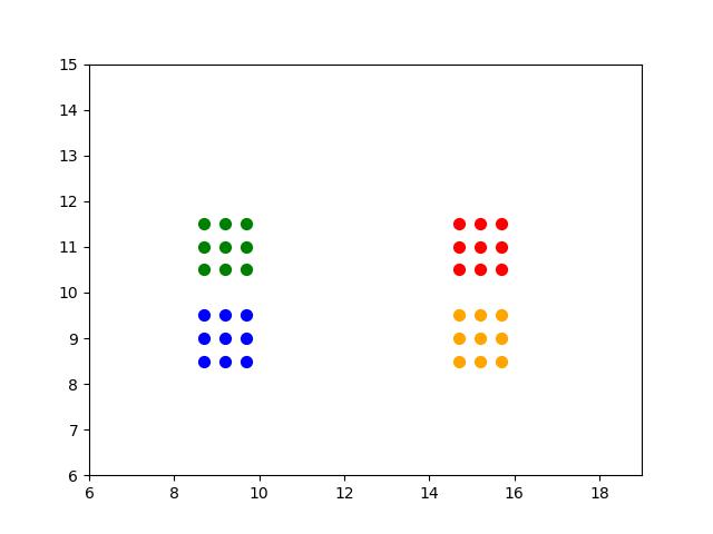
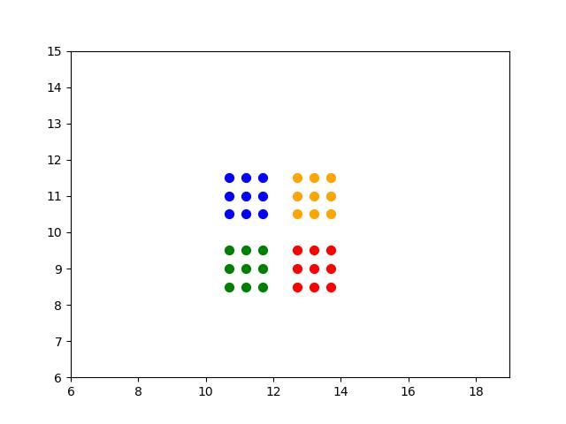
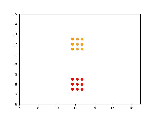
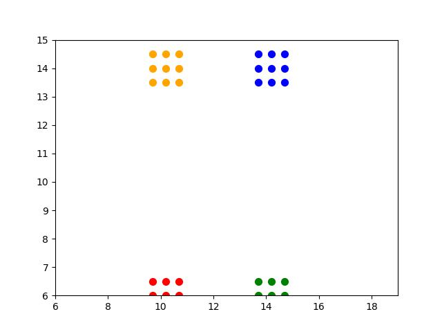
(a)K = 0	(b) K = 2	(c) K = 4	(d) K = 5	(e) K = 7

Figure 5: Plot of the data distribution of the synthetic dataset with respect to varying values of $K$. The synthetic dataset has four clusters. The value of $K$ determines the distance between the cluster centroids. Between values 0 and 4 the cluster separation reduces and between 5 and 7 the inter-cluster separation increases.

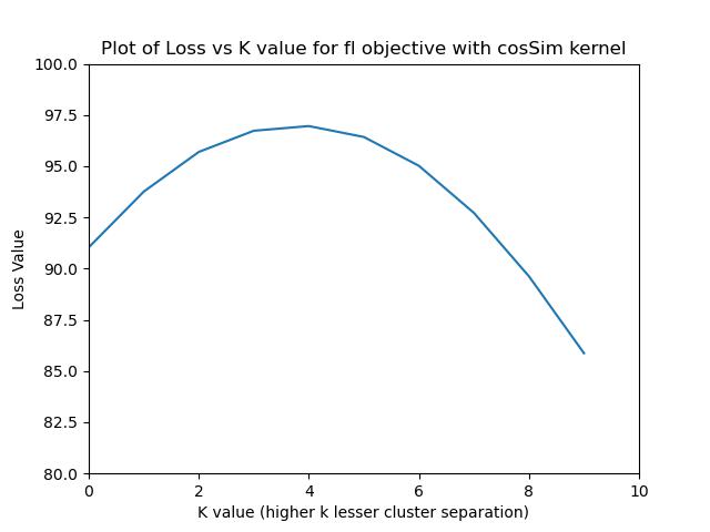
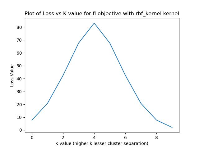
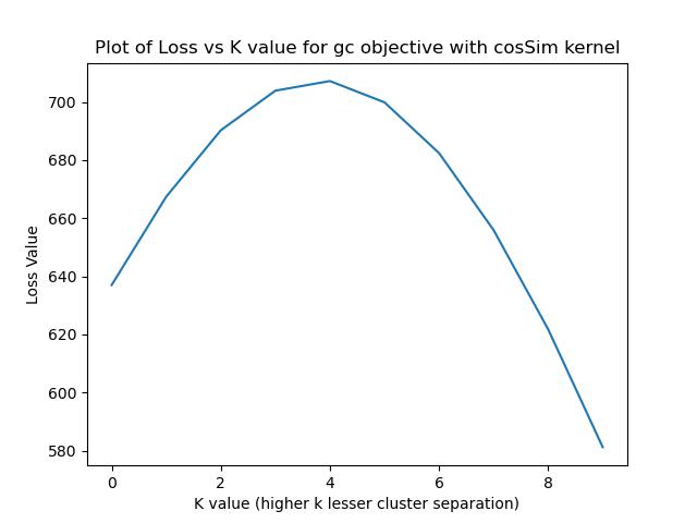
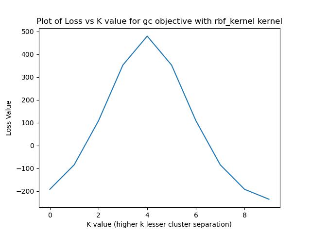
(a)FL with CosSim	(b) FL with RBF	(c) GC with CosSim	(d) GC with RBF

Figure 6: Variation in the Value of the combinatorial loss $L(\theta)$ against different values of $K$ with different similarity kernels, (a) FL objective with Cosine Similarity (CosSim) kernel, (b) FL objective with Radial Bias Field (RBF) kernel, (c) GC objective with CosSim kernel, and (d) GC objective with RBF kernel. We observe an increase in loss value with reduction in inter-cluster separation and vice-versa.

A.3 Experiments on Synthetic a dataset

This experiment characterizes the proposed submodular combinatorial objectives by demonstrating the variation in the loss value under varying inter-cluster separations and similarity kernels. The experiment proceeds with the creation of four orthogonal clusters projected on a 2-dimensional feature space with sufficient inter-cluster separation (denoted by K = 0) as shown in Figure 5(a). Over successive rounds we reduce the inter-cluster separation (by increasing the value of K from 0 through 5) such that overlaps exist between feature clusters from Figures 5(a) through (c). Further we increase the inter-cluster separation in the opposite direction (by increasing the value of K beyond 4) as shown in Figures 5(d) and (e).

For a chosen similarity kernel (either cosine-similairty or RBF [17]) we plot the calculated loss values $L(\theta)$ as in Figure 5 under varying cluster separations as discussed above. We observe that as the inter-cluster separation reduces, the value of $L(\theta)$ increases and vice-versa. This holds true irrespective of the choice of similarity kernels. Thus, by minimizing the combinatorial objective would result in large-inter feature clusters establishing the efficacy of our proposed combinatorial objectives.

Table 5: Ablation study on the effect of $\lambda$ on the performance of Graph-Cut based combinatorial objective in SCoRe.

$\lambda$	Top-1 acc
	CIFAR-10 (longtail)
0.5	83.65
1.0	89.96
1.5	87.11
2.0	85.86

A.4 Ablation Study: Effect of $\lambda$ on performance of Graph-Cut based Objective

In this section we perform experiments on the hyperparameter $\lambda$ introduced in Graph-Cut based combinatorial objective in SCoRe. The hyper-parameter $\lambda$ is applied to the sum over the penalty associated with the positive set forming tighter clusters. This parameter controls the degree of compactness of the feature cluster ensuring sufficient diversity is maintained in the feature space. For GC to be submodular it is also important for $\lambda$to be greater than or equal to 1 ($\lambda\geq 1$). For this experiment we train the two stage framework in SCoRe on the logtail CIFAR-10 dataset for 500 epochs in stage 1 with varying $\lambda$ values in range of [0.5, 2.0] and report the top-1 accuracy after stage 2 model training on the validation set of CIFAR-10. Table 5 shows that we achieve highest performance for $\lambda=1$ for longtail image classification task on the CIFAR-10 dataset. We adopt this value for all experiments conducted on GC in this paper.

A.5 Proof of Submodularity

In this section we discuss in depth the submodular counterparts of three existing objective functions in contrastive learning. We provide proofs that these functions are non-submodular in their existing forms and can be reformulated as submodular objectives through modifications without changing the characteristics of the loss function.

A.5.1 Triplet loss and Submod-Triplet loss

Triplet Loss : We first show that the Triplet loss is not necessarily submodular. The reason for this is the Triplet loss is of the form: $\sum_{i,p\in A,n\in\mathcal{V}\backslash A}D_{ipn}=\sum_{n\in\mathcal{V}}\sum_{i,p\in A}D_{ipn}-\sum_{i,p,n\in A}D_{ipn}$. Note that this is actually supermodular since $-\sum_{i,p\in A}D_{ipn}$ is submodular and $\sum_{i,p,n\in A}D_{ipn}$ is submodular. As a result, the Triplet loss is not necessarily submodular.

Submod-Triplet : Submodular Triplet loss (Submod-Triplet) is exactly the same as Graph-Cut where we use $\lambda=1$ and the similarity as the squared similarity function. Thus, this function is submodular in nature.

A.5.2 Soft-Nearest Neighbor (SNN) loss and Submod-SNN loss

SNN Loss : From the set representation of the SNN loss we can describe the objective $L(\theta,A_{k})$ as in Equation 5 . This objective function can be split into two distinct terms labelled as Term 1 and Term 2 in the equation above.

$$L(\theta,A_{k})=-\underbrace{\sum_{i\in A_{k}}[\log\sum_{j\in A_{k}}\exp(S_{ij}(\theta))}_{\text{Term 1}}-\underbrace{\log\sum_{j\in\mathcal{V}\setminus A_{k}}\exp(S_{ij}(\theta))]}_{\text{Term 2}}$$ (5)

We prove the objective to be submodular by considering two popular assumptions :
(1) The sum of submodular function over a set of classes $A_{i}$, $i\in C$, the resultant is submodular in nature.
(2) The concave over a modular function is submodular in nature.
To prove that $L(\theta,A_{k})$ is submodular in nature it is enough to show the individual terms (Term 1 and 2) to be submodular. Note that the sum of submodular functions is submodular in nature. Considering $F(A)=\sum_{j\in A_{k}}S_{j}$ for any given $i\in A_{k}$, we see that $\log\sum_{j\in A_{k}}\exp(D_{j}(\theta))$ to be modular as it is a sum over terms $\exp(D_{j}(\theta))$.
We also know from assumption (2) [31], that the concave over a modular function is submodular in nature, $\log$ being a concave function. Thus, $log\sum_{j\in A_{k}}exp(S_{j})$ is submodular function for a given $i\in A_{k}$. Unfortunately, the negative sum over a submodular function cannot be guaranteed to be submodular in nature. This renders SNN to be non-submodular in nature.

Submod-SNN Loss : The variation of SNN loss described in Table 1 can be represented as $L(\theta,A_{k})$ as shown in Equation 6. Similar to the set notation of SNN loss we can split the equation into two terms, referred to as Term 1 and Term 2 in the equation above.

$$L(\theta,A_{k})=\sum_{i\in A_{k}}[\underbrace{\log\sum_{j\in A_{k}}\exp(D_{ij}(\theta))}_{\text{Term 1}}+\underbrace{\log\sum_{j\in\mathcal{V}\setminus A_{k}}\exp(S_{ij}(\theta))}_{\text{Term 2}}]$$ (6)

Considering $F(A)=\sum_{j\in A_{k}}S_{j}$ for any given $i\in A_{k}$, we prove $\log\sum_{j\in A_{k}}\exp(D_{j}(\theta))$ to be modular, similar to the case of SNN loss. Further, using assumption (2) mentioned above we prove that the log (a concave function) over a modular function is submodular in nature. Finally, the sum of submodular functions over a set of classes $A_{k}$ is submodular according to assumption (1). Thus the term 1, $\sum_{i\in A_{k}}\log\sum_{j\in A_{k}}\exp(D_{ij}(\theta))$ in the equation of Submod-SNN is proved to be submodular in nature.

The term 2 of the equation represents the total correlation function of Graph-Cut ($L_{C_{f}}(\theta,A_{k})$). Since graph-cut function has already been proven to be submodular in [31, 19] we prove that term 2 is submodular.

Finally, since the sum of submodular functions is submodular in nature, the sum over term 1 and term 2 which constitutes $L(\theta,A_{k})$ can also be proved to be submodular.

A.5.3 N-Pairs Loss and Orthogonal Projection Loss (OPL)

In Table 1 both N-pairs loss and OPL has been identified to be submodular in nature. In this section we provide proofs to show they are submodular in nature.

N-pairs Loss : The N-pairs loss $L(\theta,A_{k})$ can be represented in set notation as described in Equation 7. Similar to SNN loss, we can split the equation into two distinct terms.

$$L(\theta,A_{k})=\underbrace{-[\sum_{i,j\in A_{k}}S_{ij}(\theta)}_{\text{Term 1}}+\underbrace{\sum_{i\in A_{k}}log(\sum_{j\in\mathcal{V}}S_{ij}(\theta)-1)]}_{\text{Term 2}}$$ (7)

The first term (Term 1) in N-pairs is a negative sum over similarities, which is submodular in nature [31]. The second term (Term 2) is a log over $\sum_{j\in\mathcal{V}}S_{ij}(\theta)-1$, which is a constant term for every training iteration as it encompases the whole ground set $\mathcal{V}$. The sum of Term 1 and Term 2 over a set $A_{k}$ is thus submodular in nature.

OPL : The loss can be represented as Equation 8 in its original form. Similar to above objectives we split the equation into two distinct terms and individually prove them to be submodular in nature.

$$L(\theta,A_{k})=(1\underbrace{-\sum_{i,j\in A_{k}}S_{ij}(\theta))}_{\text{Term 1}}+\underbrace{(\sum_{i\in A_{k}}\sum_{j\in\mathcal{V}\setminus A_{k}}S_{ij}(\theta))}_{\text{Term 2}}$$ (8)

The Term 1 represents a negative sum over similarities in set $A_{k}$ and is thus submodular in nature. The Term 2 is exactly $L_{C_{f}}$ of Graph-Cut (GC) with $\lambda=1$ and is also submodular in nature. Since the sum of two submodular functions is also submodular, $L(\theta,A_{k})$ in Equation 8 is also submodular.

A.5.4 SupCon and Submod-SupCon

SupCon : The combinatorial formulation of SupCon as in Equation 9 can be defined as a sum over the set-function $L(\theta,A_{k})$ as described in Table 1 of the main paper.

$$L(\theta,A_{k})=\underbrace{\frac{-1}{|A_{k}|}\sum_{i,j\in A_{k}}S_{ij}}_{\text{Term 1}}+\underbrace{\sum_{i\in A_{k}}\frac{1}{|A_{k}|}\log(\sum_{j\in V}exp(S_{ij})-1)}_{\text{Term 2}}$$ (9)

Similar to earlier objectives SupCon can be split into two additive terms and it is deemed enough to show that individual terms in the equations are submodular in nature. Let the marginal gain in set $A$ on addition of new element x be denoted as $F(\theta,x|A)$ where $x\in V\setminus A$. $F(\theta,x|A)$ can be written as in [31] as $F(\theta,A\cup\{x\})-F(\theta,A)$. To prove that $F(\theta,A_{i})$ is submodular it is enough to prove the condition of diminishing marginal returns, $F(\theta,x|A)\geq F(\theta,x|B)$, where $A\subseteq B\subseteq V$ and $x\in V\setminus B$. Now, considering Equation 9 we can compute the marginal gain when $\{x\}$ is added to $A$ as follows:

$$F(\theta,x|A)= F(\theta,A\cup\{x\})-F(\theta,A)$$

$$= \frac{-1}{|A\cup\{x\}|}\sum_{i,j\in A\cup\{x\}}S_{ij}+\sum_{i\in A\cup\{x\}}\frac{1}{|A\cup\{x\}|}log\Biggl{(}\sum_{j\in V}exp(S_{ij})-1\Biggr{)}-F(\theta,A)$$

$$= \Biggl{[}\frac{-1}{|A\cup\{x\}|}\sum_{i,j\in A\cup\{x\}}S_{ij}\Biggr{]}-\Biggl{[}\frac{-1}{|A|}\sum_{i,j\in A}S_{ij}\Biggr{]}$$

$$+\Biggl{[}\sum_{i\in A\cup\{x\}}\frac{1}{|A\cup\{x\}|}log\Biggl{(}\sum_{j\in V}exp(S_{ij})-1\Biggr{)}\Biggr{]}-\Biggl{[}\sum_{i\in A}\frac{1}{|A|}log\Biggl{(}\sum_{j\in V}exp(S_{ij})-1\Biggr{)}\Biggr{]}$$

To prove the first term (Term 1) to be submodular we need to show that the marginal gain on adding $\{x\}$ to set $A$ is greater than or equal to that in $B$. This can be expressed as the below inequality:

$$\Biggl{[}\frac{-1}{|A\cup\{x\}|}\sum_{i,j\in A\cup\{x\}}S_{ij}\Biggr{]}-\Biggl{[}\frac{-1}{|A|}\sum_{i,j\in A}S_{ij}\Biggr{]}\geq\Biggl{[}\frac{-1}{|B\cup\{x\}|}\sum_{i,j\in B\cup\{x\}}S_{ij}\Biggr{]}-\Biggl{[}\frac{-1}{|B|}\sum_{i,j\in B}S_{ij}\Biggr{]}$$ (10)

Simplifying the Left-Hand-Side of the equation we get:

$$= \Biggl{[}\frac{-1}{|A\cup\{x\}|}\sum_{i,j\in A\cup\{x\}}S_{ij}\Biggr{]}-\Biggl{[}\frac{-1}{|A|}\sum_{i,j\in A}S_{ij}\Biggr{]}$$

$$= \Biggl{[}\frac{-1}{|A|+1}\sum_{i,j\in A}S_{ij}\Biggr{]}+\Biggl{[}\frac{-1}{|A|+1}\sum_{i\in A}S_{ix}\Biggr{]}+\Biggl{[}\frac{-1}{|A|+1}\sum_{j\in A}S_{xj}\Biggr{]}-\Biggl{[}\frac{-1}{|A|}\sum_{i,j\in A}S_{ij}\Biggr{]}$$

$$= \Biggl{[}\frac{-2}{|A|+1}\sum_{i\in A}S_{ix}\Biggr{]}+\Biggl{[}\frac{1}{|A|(|A|+1)}\sum_{i,j\in A}S_{ij}\Biggr{]}+\Biggl{[}\frac{-1}{|A|+1}\Biggr{]}$$

Substituting the above equation in 10 we get:

$$\Biggl{[}\frac{-2}{|A|+1}\sum_{i\in A}S_{ix}\Biggr{]}+\Biggl{[}\frac{1}{|A|(|A|+1)}\sum_{i,j\in A}S_{ij}\Biggr{]}+\Biggl{[}\frac{-1}{|A|+1}\Biggr{]}$$

$$\geq\Biggl{[}\frac{-2}{|B|+1}\sum_{i\in B}S_{ix}\Biggr{]}+\Biggl{[}\frac{1}{|B|(|B|+1)}\sum_{i,j\in B}S_{ij}\Biggr{]}+\Biggl{[}\frac{-1}{|B|+1}\Biggr{]}$$

From the above inequality we see that as the size of $A$ and $B$ increases due to addition of elements to individual subsets, the inequality fails to hold. This is due to the normalization terms in the denominator which increases linearly with increase in size of the individual subsets. This renders this term to be not submodular in nature. Since, both terms in Equation 9 needs to be submodular to show $F(\theta,A_{i})$ to be submodular, we can conclude the SupCon [11] is not submodular in nature.

Submod-SupCon : The submodular SupCon as shown in Equation 11 can be split into two terms indicated as Term 1 and Term 2.

$$L(\theta,A_{k})=\underbrace{-[\sum_{i,j\in A_{k}}S_{ij}(\theta)]}_{\text{Term 1}}+\underbrace{\sum_{i\in A_{k}}[log(\sum_{j\in\mathcal{V}\setminus A_{k}}\exp(S_{ij}(\theta)))}_{\text{Term 2}}]$$ (11)

The Term 1 of Submod-SupCon is a negative sum over similarities of set $A_{k}$ and is thus submodular. The Term 2 of the equation is also submodular as it is a concave over the modular term $\sum_{j\in\mathcal{V}\setminus A_{k}}\exp(S_{ij}(\theta)$, with $\log$ being a concave function. Thus, Submod-SupCon is also submodular as the sum of two submodular functions is submodular in nature.

References

- [1] Alex Krizhevsky, Ilya Sutskever, and Geoffrey E Hinton. Imagenet classification with deep convolutional neural networks. In Advances in Neural Information Processing Systems, 2012.
- [2] Kaiming He, Xiangyu Zhang, Shaoqing Ren, and Jian Sun. Deep residual learning for Image Recognition. In IEEE Conf. on Computer Vision and Pattern Recognition (CVPR), 2016.
- [3] Karen Simonyan and Andrew Zisserman. Very deep convolutional networks for large-scale image recognition. In Intl. Conf. on Learning Representations, 2015.
- [4] Eric Baum and Frank Wilczek. Supervised learning of probability distributions by neural networks. In Neural Information Processing Systems, 1987.
- [5] Xiaobin Li and Weiqiang Wang. Learning discriminative features via weights-biased softmax loss. Pattern Recognition, 2020.
- [6] Kanchana Ranasinghe, Muzammal Naseer, Munawar Hayat, Salman Khan, and Fahad Shahbaz Khan. Orthogonal projection loss. In Proceedings of the IEEE/CVF International Conference on Computer Vision (ICCV), 2021.
- [7] Jiankang Deng, Jia Guo, Niannan Xue, and Stefanos Zafeiriou. Arcface: Additive angular margin loss for deep face recognition. In Proceedings of the IEEE/CVF Conference on Computer Vision and Pattern Recognition, pages 4690–4699, 2019.
- [8] Hao Wang, Yitong Wang, Zheng Zhou, Xing Ji, Dihong Gong, Jingchao Zhou, Zhifeng Li, and Wei Liu. Cosface: Large margin cosine loss for deep face recognition. In Proceedings of the IEEE Conference on Computer Vision and Pattern Recognition (CVPR), June 2018.
- [9] Florian Schroff, Dmitry Kalenichenko, and James Philbin. Facenet: A unified embedding for face recognition and clustering. In IEEE Conf. on Computer Vision and Pattern Recognition (CVPR), 2015.
- [10] Kihyuk Sohn. Improved deep metric learning with multi-class n-pair loss objective. In Advances in Neural Inf. Processing Systems, 2016.
- [11] Prannay Khosla, Piotr Teterwak, Chen Wang, Aaron Sarna, Yonglong Tian, Phillip Isola, Aaron Maschinot, Ce Liu, and Dilip Krishnan. Supervised contrastive learning. In Advances in Neural Information Processing Systems, 2020.
- [12] Ting Chen, Simon Kornblith, Mohammad Norouzi, and Geoffrey Hinton. A simple framework for contrastive learning of visual representations. Intl. Conf. on Machine Learning (ICML), 2020.
- [13] Satoru Fujishige. Submodular functions and optimization. Elsevier, 2005.
- [14] V. Kaushal, R. Iyer, K. Doctor, A. Sahoo, P. Dubal, S. Kothawade, R. Mahadev, K. Dargan, and G. Ramakrishnan. Demystifying multi-faceted video summarization: Tradeoff between diversity, representation, coverage and importance. In 2019 IEEE Winter Conference on Applications of Computer Vision (WACV), pages 452–461, 2019.
- [15] Suraj Kothawade, Saikat Ghosh, Sumit Shekhar, Yu Xiang, and Rishabh K. Iyer. Talisman: Targeted active learning for object detection with rare classes and slices using submodular mutual information. In Computer Vision - ECCV 2022 - 17th European Conference, 2022.
- [16] Suraj Kothawade, Nathan Beck, Krishnateja Killamsetty, and Rishabh Iyer. SIMILAR: Submodular information measures based active learning in realistic scenarios. Advances in Neural Information Processing Systems, 34, 2021.
- [17] Krishnateja Killamsetty, Durga S, Ganesh Ramakrishnan, Abir De, and Rishabh Iyer. Grad-match: Gradient matching based data subset selection for efficient deep model training. In Marina Meila and Tong Zhang, editors, Proceedings of the 38th International Conference on Machine Learning, volume 139 of Proceedings of Machine Learning Research, pages 5464–5474. PMLR, 18–24 Jul 2021.
- [18] Athresh Karanam, Krishnateja Killamsetty, Harsha Kokel, and Rishabh Iyer. Orient: Submodular mutual information measures for data subset selection under distribution shift. In S. Koyejo, S. Mohamed, A. Agarwal, D. Belgrave, K. Cho, and A. Oh, editors, Advances in Neural Information Processing Systems, volume 35, pages 31796–31808. Curran Associates, Inc., 2022.
- [19] Rishabh Iyer, Ninad Khargonkar, Jeff Bilmes, and Himanshu Asnani. Generalized submodular information measures: Theoretical properties, examples, optimization algorithms, and applications. IEEE Transactions on Information Theory, 68(2):752–781, 2022.
- [20] Suraj Kothawade, Vishal Kaushal, Ganesh Ramakrishnan, Jeff A. Bilmes, and Rishabh K. Iyer. PRISM: A rich class of parameterized submodular information measures for guided data subset selection. In Thirty-Sixth AAAI Conference on Artificial Intelligence, AAAI, pages 10238–10246, 2022.
- [21] Jiancheng Yang, Rui Shi, Donglai Wei, Zequan Liu, Lin Zhao, Bilian Ke, Hanspeter Pfister, and Bingbing Ni. Medmnist v2-a large-scale lightweight benchmark for 2d and 3d biomedical image classification. Scientific Data, 10(1):41, 2023.
- [22] G. Varma, A. Subramanian, A. Namboodiri, M. Chandraker, and C. V. Jawahar. IDD: A dataset for exploring problems of autonomous navigation in unconstrained environments. In IEEE Winter Conf. on Applications of Computer Vision (WACV), pages 1743–1751, 2019.
- [23] David E Rumelhart, Geoffrey E Hinton, and Ronald J Williams. Learning representations by back-propagating errors. nature, 323(6088):533–536, 1986.
- [24] Xun Wang, Xintong Han, Weilin Huang, Dengke Dong, and Matthew R Scott. Multi-similarity loss with general pair weighting for deep metric learning. In Proc. of the IEEE Conf. on Computer Vision and Pattern Recognition, 2019.
- [25] Yandong Wen, Kaipeng Zhang, Zhifeng Li, and Yu Qiao. A discriminative feature learning approach for deep face recognition. In Bastian Leibe, Jiri Matas, Nicu Sebe, and Max Welling, editors, Computer Vision – ECCV 2016, pages 499–515, 2016.
- [26] Michael Gutmann and Aapo Hyvärinen. Noise-contrastive estimation: A new estimation principle for unnormalized statistical models. In Proceedings of the Thirteenth International Conference on Artificial Intelligence and Statistics, 2010.
- [27] Kaiming He, Haoqi Fan, Yuxin Wu, Saining Xie, and Ross Girshick. Momentum contrast for unsupervised visual representation learning. In 2020 IEEE/CVF Conference on Computer Vision and Pattern Recognition (CVPR), 2020.
- [28] Xinlei Chen, Haoqi Fan, Ross Girshick, and Kaiming He. Improved baselines with momentum contrastive learning. arXiv preprint arXiv:2003.04297, 2020.
- [29] Hyun Oh Song, Yu Xiang, Stefanie Jegelka, and Silvio Savarese. Deep metric learning via lifted structured feature embedding. In Computer Vision and Pattern Recognition (CVPR), 2016.
- [30] Nicholas Frosst, Nicolas Papernot, and Geoffrey E. Hinton. Analyzing and improving representations with the soft nearest neighbor loss. In International Conference on Machine Learning, 2019.
- [31] Satoru Fujishige. Submodular Functions and Optimization, volume 58. Elsevier, 2005.
- [32] Hyun Oh Song, Stefanie Jegelka, Vivek Rathod, and Kevin Murphy. Deep metric learning via facility location. In Proceedings of the IEEE Conference on Computer Vision and Pattern Recognition (CVPR), July 2017.
- [33] Alex Krizhevsky. Learning multiple layers of features from tiny images. 2009.
- [34] Shaoqing Ren, Kaiming He, Ross B. Girshick, and J. Sun. Faster r-cnn: Towards real-time object detection with region proposal networks. IEEE Transactions on Pattern Analysis and Machine Intelligence, 2015.
- [35] T. Lin, P. Goyal, R. Girshick, K. He, and P. Dollár. Focal Loss for dense object detection. In IEEE Intl. Conf. on Computer Vision (ICCV), pages 2999–3007, 2017.
- [36] Joseph Redmon and Ali Farhadi. YOLOv3: An Incremental Improvement. CoRR, abs/1804.02767, 2018.
- [37] P. Hurtík, Vojtech Molek, J. Hula, M. Vajgl, Pavel Vlasánek, and Tomas Nejezchleba. Poly-YOLO: Higher speed, more precise detection and instance segmentation for yolov3. ArXiv, abs/2005.13243, 2020.
- [38] K. He, G. Gkioxari, P. Dollár, and R. Girshick. Mask R-CNN. In IEEE Intl. Conf. on Computer Vision (ICCV), 2017.
- [39] Anay Majee, Kshitij Agrawal, and Anbumani Subramanian. Few-Shot Learning For Road Object Detection. In AAAI Workshop on Meta-Learning and MetaDL Challenge, volume 140, pages 115–126, 2021.