3D Reconstruction in Noisy Agricultural Environments:
A Bayesian Optimization Perspective for View Planning

Abstract

3D reconstruction is a fundamental task in robotics that gained attention due to its major impact in a wide variety of practical settings, including agriculture, underwater, and urban environments. An important approach for this task, known as view planning, is to judiciously place a number of cameras in positions that maximize the visual information improving the resulting 3D reconstruction. Circumventing the need for a large number of arbitrary images, geometric criteria can be applied to select fewer yet more informative images to markedly improve the 3D reconstruction performance. Nonetheless, incorporating the noise of the environment that exists in various real-world scenarios into these criteria may be challenging, particularly when prior information about the noise is not provided. To that end, this work advocates a novel geometric function that accounts for the existing noise, relying solely on a relatively small number of noise realizations without requiring its closed-form expression. With no analytic expression of the geometric function, this work puts forth a Bayesian optimization algorithm for accurate 3D reconstruction in the presence of noise. Numerical tests on noisy agricultural environments showcase the impressive merits of the proposed approach for 3D reconstruction with even a small number of available cameras.

I Introduction

Acquiring visual information is a key component in robotics for scene understanding, planning, and decision-making. In particular, the acquisition of 3D information, known as 3D scene reconstruction, has gained popularity in different robotic settings, including agricultural [1, 2, 3, 4], underwater [5], and urban [6, 7] environments. This task involves deciding the placement of a set of available cameras in the 3D space in order to acquire the necessary information and effectively reconstruct an area of interest. This problem is termed view planning (VP) [8, 9], where determining the camera placement can be carried out offline given a fixed number of cameras and a static model of the environment so that the information gain of each camera can be assessed. Thus, a VP approach can significantly improve the quality of the 3D reconstruction (usually expressed as point clouds) when compared to an arbitrary set of camera placements, which usually results in low-density point clouds.

Nonetheless, obtaining the optimal camera placement may be challenging when the size of the environment becomes large; see e.g., urban environments. To cope with this challenge, existing methods have formulated VP as a discrete optimization problem in order to reduce the space of feasible solutions [1, 10]. A class of methods employed to solve the VP problem is based on search algorithms; e.g., [1, 6]. Recently, neural networks have been utilized in the VP setting to get an estimate of the function that maps any camera placement to its corresponding reconstruction quality [11]. The reward functions that provide the evaluation of the different camera settings, can be categorized into geometric [1] or occupancy maps [11], based on the application.

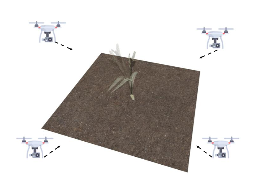
Figure 1: Example of a noisy environment with four drones aiming to carry out the 3D reconstruction task (drone image ).

Albeit interesting, all these approaches do not account for any type of environmental noise, which can prove to be important when modeling the environment and can significantly affect the VP performance in practical settings. In Fig. 2, there is an example of how the noise affects the geometry of the environment in VP. However, forming an analytic expression of the noise may be a challenging task, particularly when the number of noise realizations is not sufficient. With no analytic expression of the noise, the expression of the reward function that incorporates the noise also becomes unknown, and thus conventional optimization techniques including gradient-based solvers, may not be applicable.

This motivates the use of the Bayesian optimization (BO) paradigm that aims at optimizing a black-box (unknown) function by leveraging a (typically small) number of function evaluations to form a probabilistic surrogate model that will guide the selection of new query points [12]. Relying on the surrogate model, the so-termed acquisition function (AF), typically expressed in closed-form, is used to sequentially select the next query points in the optimization process. BO has been adopted in a range of practical settings including hyperparameter tuning [13], drug discovery [14] and robotic based tasks [15, 16, 17] to name a few. Nonetheless, none of the existing works has considered adopting BO in the VP problem under noisy environments.

This paper presents a novel approach for modeling and optimizing the reward function of the VP problem in order to effectively and efficiently reconstruct an area of interest in the presence of noise. The contributions of this work can be summarized in the following directions

• To the best of our knowledge, this work is the first to incorporate existing noise in the reward function of a VP problem for 3D reconstruction.

• Without knowledge of the analytic expression of the noise incorporated in the reward function, the proposed approach relies solely on a small number of noise realizations to carry out the 3D reconstruction task.

• To optimize the reward function with unknown closed-form expression, the present work is the first to introduce well-motivated BO methods for the VP problem.

• Compared to most existing approaches that require discretization of the search space in order to be tractable, this work focuses on a continuous optimization problem that considers the entire search space.

• Promising experimental results on three different agriculture-based environments demonstrate the effectiveness of the proposed approach for accurate 3D reconstruction with a limited number of available cameras.

II Related Work

II-A View Planning

Initial works of VP [8, 9] aim at placing cameras in an optimal way that maximizes the gain of information about the environment, to successfully carry out the 3D reconstruction task. In order to reduce the complexity of the search space, which may be intractable in large environments, several works have modeled the problem in a discrete manner [1, 11, 8, 9]. However, this discrete formulation is known to be NP-complete, as shown in [9], leading to the use of sampling-based search methods [1] or approximate algorithms that require two or more optimization phases [10].

Besides an affordable complexity, a critical component in the VP optimization problem is the proper selection of the reward function. Given the information about the environment, two different types of reward functions have been mainly explored, namely occupancy maps and geometric evaluations. Although offering a simple representation of the environment, occupancy maps may reduce the quality of the 3D reconstruction [18, 11, 19]. On the other hand, geometric functions typically achieve more dense point clouds in the resulting reconstruction by imposing more constraints in the view selection process [1, 3, 4]. In our work, we will focus on a geometric function since we aim to improve the reliability of the 3D reconstruction.

Finally, an aspect of great interest in real-world settings is the existing noise of the environment. Although the information of the static environment is given, in several applications there are many parameters, such as the wind, that may alter the representation of the environment, hence affecting the outcome of the 3D reconstruction. Therefore, it is of paramount importance to incorporate these types of disturbances in the selection of the views to achieve the best reconstruction.

Despite the effectiveness of the aforementioned VP approaches in noise-free environments, none of them has considered the effects of the noise in the VP process, or the merits of a continuous formulation over a discrete one where any position in the 3D space can be explored.

II-B Bayesian Optimization

Bayesian optimization (BO) provides a principled framework to optimize a black-box or costly to evaluate function, by judiciously exploiting a number of function values to build a surrogate model, that allows for the sequential acquisition of new points. The key components of BO are (i) the selection of a probabilistic surrogate model and (ii) the design of the AF to select new points to query on-the-fly. Gaussian processes (GPs) have been extensively adopted as a nonparametric Bayesian surrogate model in a range of BO applications due to their well-documented merits in learning an unknown function along with its probability density function (pdf) in a sample-efficient manner [20, 12]. Although interesting and effective in several practical settings, their performance hinges on the proper selection of the kernel function to evaluate the pairwise similarity of different input points, whose selection is a non-trivial task. To cope with this challenge existing works adaptively learn the kernel as new data arrive on-the-fly; see e.g., [21, 22, 23, 24, 25]. Capitalizing on GP-based surrogate models, several AFs have been designed including Thompson sampling [26], expected improvement (EI) [27] or upper confidence bound [28] to name a few. These AFs are expressed in closed-form, they are easy to optimize and have well-documented merits in balancing exploration and exploitation of the search space.

III Problem Formulation

The objective of the VP problem is to find an optimal camera setup that will maximize the information that can be extracted from a given environment in order to assist the 3D reconstruction task. Specifically, given a number of cameras $N$, and a point cloud $\{\mathbf{p}\}_{i=1}^{\pazocal{P}}\subseteq\mathbb{R}^{3}$, sampled from the given representation of the environment, the goal is to find

$$\mathbf{z}^{*}=\operatorname*{arg\,max}_{\mathbf{z}\in\pazocal{Z}}\;r(\mathbf{z};\mathbf{p}_{1},\dots,\mathbf{p}{P})$$ (1)

where $\mathbf{z}:=[\mathbf{x}_{1},\dots,\mathbf{x}_{N}]$, with $\{\mathbf{x}_{i}\}_{i=1}^{N}\subseteq\mathbb{R}^{6}$ denoting each camera feature vector and $\pazocal{Z}$ is the set of feasible solutions. In particular, $\mathbf{x}_{i}=[\mathbf{c}_{i},\mathbf{v}_{i}]$ with $\mathbf{c}_{i}\in\mathbb{R}^{3}$ and $\mathbf{v}_{i}\in\mathbb{R}^{3}$ containing the information of the location, and the orientation of the $i^{\text{th}}$ camera. The reward function $r(\cdot)$ represents the quality of the 3D reconstruction.

Following the discrete geometrical formulation of [1] for the $r(\cdot)$ function, an extended version of the $r(\cdot)$ in continuous space is expressed as

$$r(\mathbf{z})=\frac{1}{\pazocal{P}\pazocal{S}}\sum_{\begin{subarray}{c}\mathbf{p}\in\pazocal{P}\\ (\mathbf{c}_{i},\mathbf{v}_{i},\mathbf{c}_{j},\mathbf{v}_{j})\in\mathbf{z}\end{subarray}}f(\mathbf{c}_{i},\mathbf{c}_{j},\mathbf{p})g(\mathbf{c}_{i},\mathbf{v}_{i},\mathbf{c}_{j},\mathbf{v}_{j},\mathbf{p})$$ (2)

where $f(\cdot)$ indicates the reconstruction quality per point $\mathbf{p}$ from the camera location pair $(\mathbf{c}_{i},\mathbf{c}_{j})$, $g(\cdot)$ represents the geometric constraints for each $(\mathbf{c}_{i},\mathbf{v}_{i}),(\mathbf{c}_{j},\mathbf{v}_{j})$ camera pair, and $\pazocal{S}$ is the total number of $(i,j)$ pairs.

The geometric reconstruction quality, defined by $f(\cdot)$, relies on the angle between the vectors $(\mathbf{c}_{i}-\mathbf{p}),(\mathbf{c}_{j}-\mathbf{p})$ $\forall(i,j)$. When the angle value increases, the reconstruction quality error of $\mathbf{p}$ becomes smaller. This can be expressed by the sine between these two vectors as

$$f(\mathbf{c}_{i},\mathbf{c}_{j},\mathbf{p})=\frac{\norm{(\mathbf{c}_{i}-\mathbf{p})\times(\mathbf{c}_{j}-\mathbf{p})}}{\norm{\mathbf{c}_{i}-\mathbf{p}}\norm{\mathbf{c}_{j}-\mathbf{p}}}$$ (3)

In order for Eqn. (3) to provide an accurate estimate of the reconstruction quality for each point $\mathbf{p}$, two conditions need to be satisfied. The first focuses on the number of those points that are able to be seen from each camera $(\mathbf{c}_{i},\mathbf{v}_{i})$, and the second on the ability of all the camera pairs $(\mathbf{c}_{i},\mathbf{v}_{i}),(\mathbf{c}_{j},\mathbf{v}_{j})$ to gain 3D information of the common viewed points $\mathbf{p}$. Specifically, the function $g(\cdot)$ has the form

$$g(\mathbf{c}_{i},\mathbf{v}_{i},\mathbf{c}_{j},\mathbf{v}_{j},\mathbf{p})=\mathds{1}(cond_{1}^{i})\mathds{1}(cond_{1}^{j})\mathds{1}(cond_{2}^{i,j})$$ (4)

where $\mathds{1}(\cdot)$ is the indicator function, returning value 1 when the input condition is satisfied and 0 otherwise. The conditions ($cond_{1}^{i},cond_{2}^{i,j}$) regarding each camera pair ($i,j$) are defined as

$$cond_{1}^{i}:=\cos(\phi_{1}^{i})-\cos(\frac{FoV}{2})\geq 0$$ (5)

$$cond_{2}^{i,j}:=\cos(\phi_{2}^{i,j})-\cos(\theta_{match})\geq 0$$ (6)

where $\cos(\phi_{1}^{i}):=\frac{(\mathbf{c_{i}}-\mathbf{p})\cdot\mathbf{v_{i}}}{\norm{\mathbf{c_{i}}-\mathbf{p}}\norm{\mathbf{v_{i}}}}$, $\cos(\phi_{2}^{i,j}):=\frac{(\mathbf{c}_{i}-\mathbf{p})\cdot(\mathbf{c}_{j}-\mathbf{p})}{\norm{\mathbf{c}_{i}-\mathbf{p}}\norm{\mathbf{c}_{j}-\mathbf{p}}}$, $FoV$ is the camera field-of-view parameter and $\theta_{match}$ the maximum angle between the vectors ($\mathbf{c}_{i}-\mathbf{p}$), ($\mathbf{c}_{j}-\mathbf{p}$), so that to reconstruct the point $\mathbf{p}$.

The reward function in Eqn. (1), although formulating the VP problem, does not account for real-world scenarios where there is noise in the environment. To cope with this limitation, we assume that each point $\mathbf{p}$ under the noisy environment becomes $\tilde{\mathbf{p}}=h(\mathbf{p})$, where the function $h(\cdot)$ models the effect of the noise, whose expression is considered unknown. For instance, the function $h(\cdot)$ may have a linear form of $h(\mathbf{p})=\mathbf{p}+\mathbf{n}$, with $\mathbf{n}$ following a distribution $\mathscr{D}$ parameterized by $\omega$; that is $\mathbf{n}\sim\mathscr{D}(\omega)$. Taking into account the function $h(\cdot)$, Eqn. (2) becomes

$$\begin{split}\tilde{r}(\mathbf{z})=\frac{1}{\pazocal{P}\pazocal{S}}\sum_{\begin{subarray}{c}\mathbf{p}\in\pazocal{P}\\ (\mathbf{c}_{i},\mathbf{v}_{i},\mathbf{c}_{j},\mathbf{v}_{j})\in\mathbf{z}\end{subarray}}f(\mathbf{c}_{i},\mathbf{c}_{j},\tilde{\mathbf{p}})g(\mathbf{c}_{i},\mathbf{v}_{i},\mathbf{c}_{j},\mathbf{v}_{j},\tilde{\mathbf{p}}).\end{split}$$ (7)

Finally, the VP optimization problem turns into

$$\mathbf{z}^{*}=\operatorname*{arg\,max}_{\mathbf{z}\in\pazocal{Z}}\tilde{r}(\mathbf{z};\tilde{\mathbf{p}}_{1},\dots,\tilde{\mathbf{p}}{P}).$$ (8)

It is worth noticing that the analytic expression of the objective function in Eqn. (8) becomes unknown when apriori information about the function $h(\cdot)$ is not provided. With no analytic expression at hand, conventional gradient-based solvers are not applicable for obtaining $\mathbf{z}^{*}$. This motivates well the BO paradigm that offers principled methods to effectively optimize black-box functions in a data-efficient manner, as outlined next.

Figure 2: Bayesian optimization with expected improvement in a nutshell.

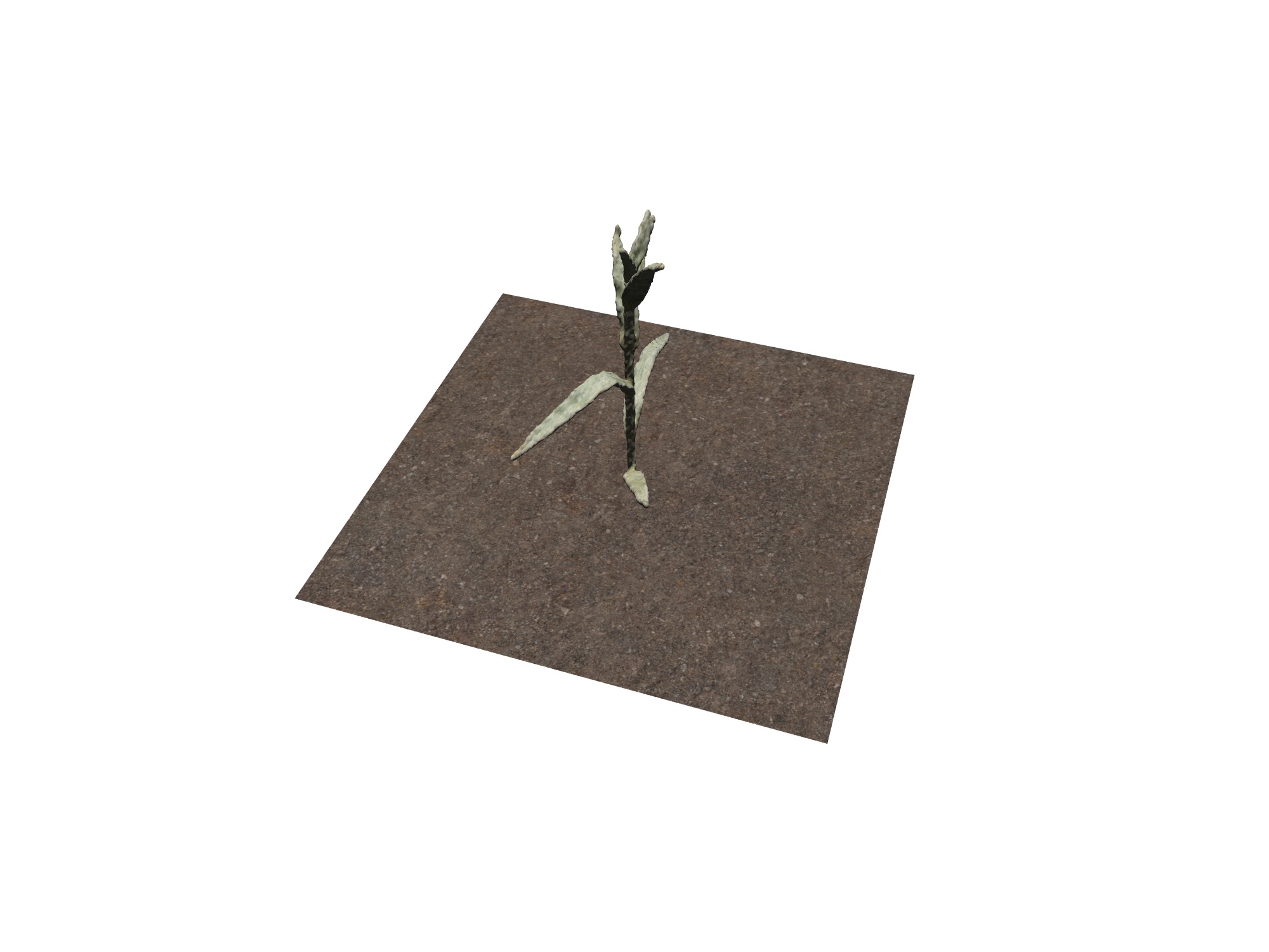
(a)

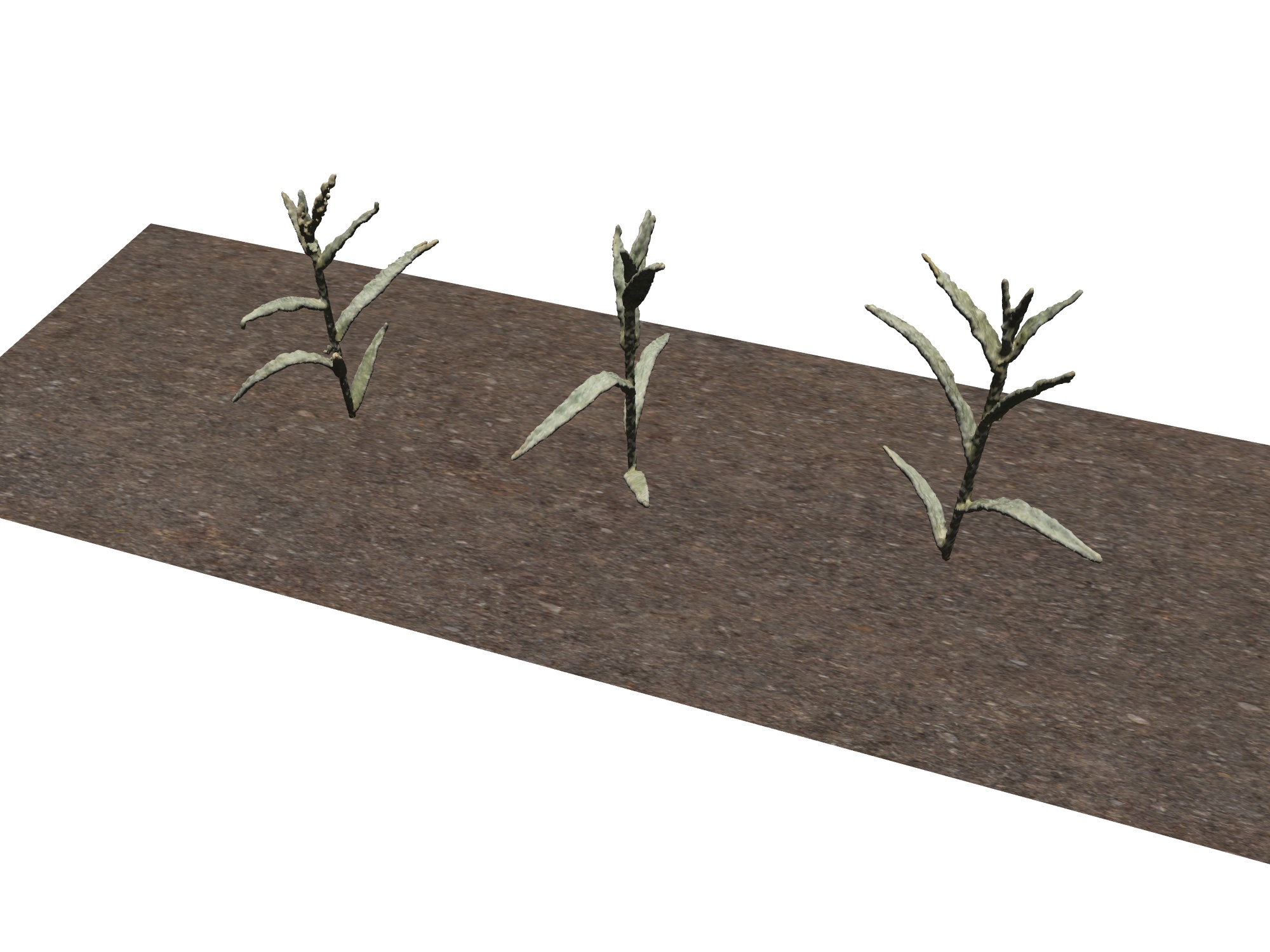
(b)

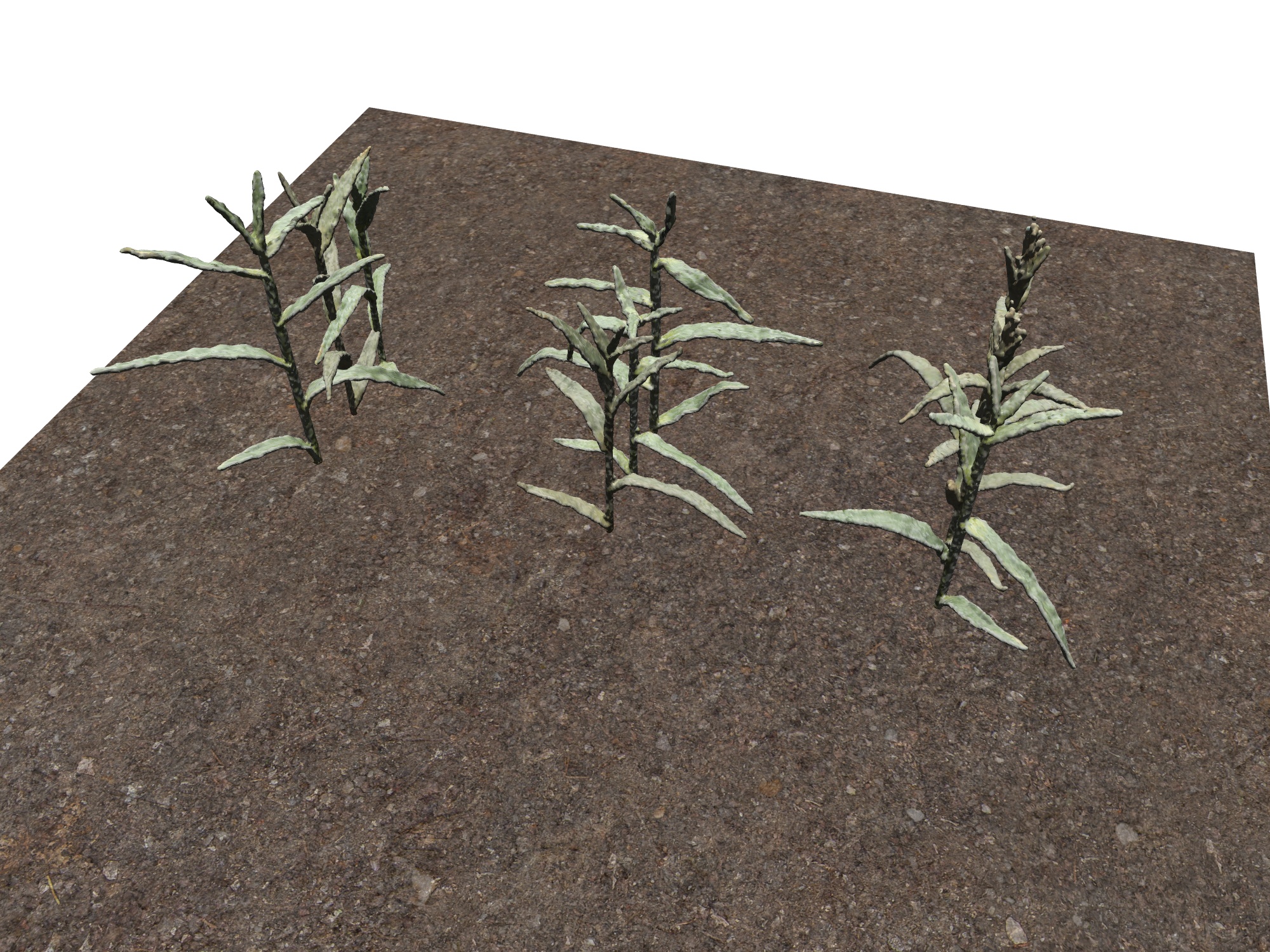
(c)

Figure 3: Environmental agricultural scenarios.

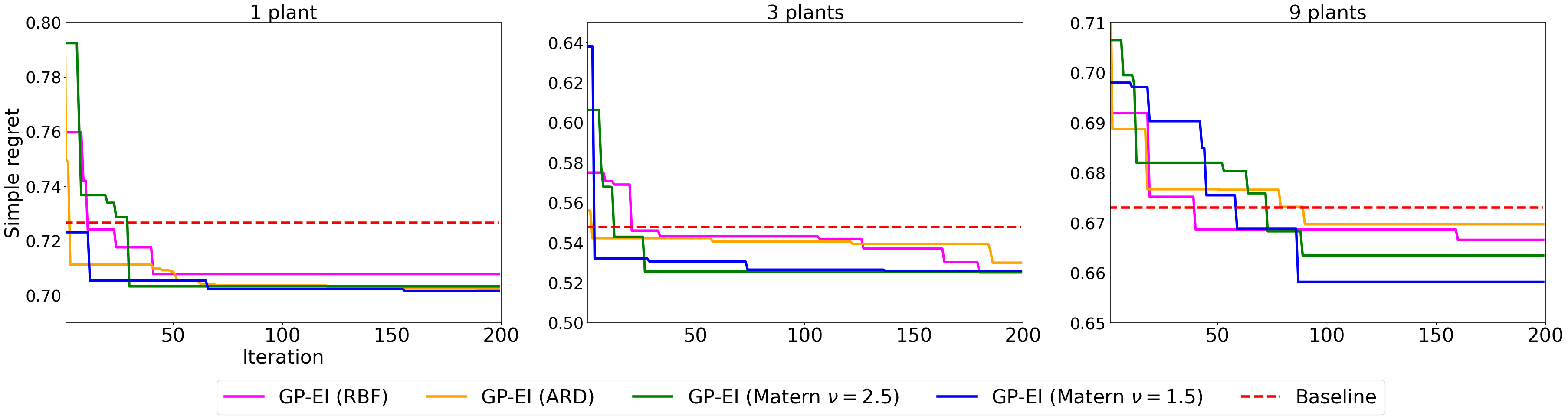
Figure 4: Simple regret for (a) 1-plant, (b) 3-plants, and (c) 9-plants scenarios.

IV Optimization Method

Relying on a given budget of input-output data pairs $\pazocal{D}_{t}:=\{(\mathbf{z}_{\tau},\tilde{r}_{\tau})\}_{\tau=1}^{t}$ with $\tilde{r}_{\tau}:=\tilde{r}(\mathbf{z}_{\tau})$, BO capitalizes on a probabilistic surrogate model $p(\tilde{r}(\mathbf{z})|\pazocal{D}_{t})$ for $\tilde{r}$, that guides the acquisition of the next query input $\mathbf{z}_{t+1}$. Specifically, each iteration of the BO process follows a two-step approach; that is (i) update $p(\tilde{r}(\mathbf{z})|\pazocal{D}_{t})$ using $\pazocal{D}_{t}$ and (ii) obtain $\mathbf{z}_{t+1}\!=\!\underset{\mathbf{z}\in\pazocal{Z}}{\arg\max}\ \alpha_{t+1}(\mathbf{z}|\pazocal{D}_{t})$ using $p(\tilde{r}(\mathbf{z})|\pazocal{D}_{t})$. The so-termed acquisition function (AF) $\alpha_{t+1}(\mathbf{z}|\pazocal{D}_{t})$, often expressed in closed-form, is chosen so as to balance exploration and exploitation of the search space [12]. There are several choices for both $p(\tilde{r}(\mathbf{z})|\pazocal{D}_{t})$ and $\alpha_{t+1}(\mathbf{z}|\pazocal{D}_{t})$. In this work, we will focus on the Gaussian process (GP) based surrogate model that has been extensively used in a gamut of BO applications; see e.g., [12, 21], and will use expected improvement (EI) as the AF.

Belonging to the family of nonparametric Bayesian approaches, GPs offer a principled framework to learn an unknown function with well-quantified uncertainty, which can readily guide the acquisition of new query input points. Learning with GPs begins with the assumption that a GP prior is postulated over the function $\tilde{r}(\mathbf{z})$ as $\tilde{r}\sim\pazocal{GP}(0,\kappa(\mathbf{z},\mathbf{z}^{\prime}))$, with $\kappa(\mathbf{z},\mathbf{z}^{\prime})$ representing a positive-definite kernel function that measures the pairwise similarity between $\mathbf{z}$ and $\mathbf{z}^{\prime}$. This means that the random vector $\tilde{\mathbf{r}}_{t}:=[\tilde{r}(\mathbf{z}_{1}),\ldots,\tilde{r}(\mathbf{z}_{t})]^{\top}$ that consists of all function values at inputs $\mathbf{Z}_{t}:=\left[\mathbf{z}_{1},\ldots,\mathbf{z}_{t}\right]^{\top}$ is Gaussian distributed as $\tilde{\mathbf{r}}_{t}\sim\pazocal{N}(\tilde{\mathbf{r}}_{t};{\bf 0}_{t},{\bf K}_{t})(\forall t)$, where ${\bf K}_{t}$ is the $t\times t$ kernel (covariance) matrix whose $(i,j)$th element is $[{\bf K}_{t}]_{i,j}={\rm cov}(\tilde{r}(\mathbf{z}_{i}),\tilde{r}(\mathbf{z}_{j})):=\kappa(\mathbf{z}_{i},\mathbf{z}_{j})$ [20].

With $\mathbf{y}_{t}:=[y_{1},\ldots,y_{t}]^{\top}$ denoting the (possibly) noisy output vector where $y_{\tau}=\tilde{r}({\bf z}_{\tau})+n_{\tau}$ ($\forall\tau$) and $n_{\tau}\sim\pazocal{N}(n_{\tau};0,\sigma_{n}^{2})$ is white Gaussian noise uncorrelated across $\tau$, learning with GPs follows the assumption that the batch conditional likelihood $p(\mathbf{y}_{t}|\tilde{\mathbf{r}}_{t};\mathbf{Z}_{t})$ is factored as

$$p(\mathbf{y}_{t}|\tilde{\mathbf{r}}_{t};\mathbf{Z}_{t})\!=\!\prod_{\tau=1}^{t}p(y_{\tau}|\tilde{r}(\mathbf{z}_{\tau}))\!=\!\prod_{\tau=1}^{t}\!\pazocal{N}(y_{\tau};\tilde{r}(\mathbf{z}_{\tau}),\sigma_{n}^{2}).$$

With the GP prior and the batch likelihood at hand, one can write the joint pdf of $\mathbf{y}_{t}$ and $\tilde{r}(\mathbf{z})$ for any input (cameras placement) vector $\mathbf{z}$ as

$$\begin{bmatrix}\mathbf{y}_{t}\\ \tilde{r}({\bf z})\end{bmatrix}\!\sim\!\pazocal{N}\!\left(\!\mathbf{0}_{t+1},\!\!\begin{bmatrix}\mathbf{K}_{t}\!+\!\sigma_{n}^{2}\mathbf{I}_{t}&\mathbf{k}_{t}({\bf z})\\ \mathbf{k}_{t}^{\top}({\bf z})&\kappa(\mathbf{z},\mathbf{z})\!+\!\sigma_{n}^{2}\end{bmatrix}\!\right)$$

where $\mathbf{k}_{t}({\bf z}):=[\kappa(\mathbf{z}_{1},\mathbf{z}),\ldots,\kappa(\mathbf{z}_{t},\mathbf{z})]^{\top}$ [20]. Then, it can be shown that the function posterior pdf of $\tilde{r}(\mathbf{z})$ at any input $\mathbf{z}$ is Gaussian distributed as

$$p(\tilde{r}(\mathbf{z})|\pazocal{D}_{t})=\pazocal{N}(\tilde{r}(\mathbf{z});\mu_{t}(\mathbf{z}),\sigma_{t}^{2}(\mathbf{z}))$$ (9)

with mean and variance given in closed form as described in [20]

$$\mu_{t}({\bf z}) =\mathbf{k}_{t}^{\top}({\bf z})(\mathbf{K}_{t}+\sigma_{n}^{2}\mathbf{I}_{t})^{-1}\mathbf{y}_{t}$$ (10a)

$$\sigma_{t}^{2}({\bf z}) =\!\kappa(\mathbf{z},\mathbf{z})\!-\!\mathbf{k}_{t}^{\top}({\bf z})(\mathbf{K}_{t}\!+\!\sigma_{n}^{2}\mathbf{I}_{t})^{-1}\mathbf{k}_{t}({\bf z}).$$ (10b)

Note that the mean in Eqn. (10a) provides a point estimate of the function $\tilde{r}$ evaluated at $\mathbf{z}$ and the variance in Eqn. (10b) quantifies the associated uncertainty.

Leveraging the posterior pdf $p(\tilde{r}(\mathbf{z})|\pazocal{D}_{t})$ one can select the next input query point $\mathbf{z}_{t+1}$ using the EI AF as follows [27]

$$\mathbf{z}_{t+1}=\underset{\mathbf{z}\in\pazocal{Z}}{\arg\max}\ \mathbb{E}_{p(\tilde{r}(\mathbf{z})|\pazocal{D}_{t})}[\text{max}(0,\tilde{r}(\mathbf{z})-\hat{\tilde{r}}_{t}^{\text{max}})]$$ (11)

with $\hat{\tilde{r}}_{t}^{\text{max}}$ denoting an estimate of the maximum value of $\tilde{r}(\cdot)$ at iteration $t$. A typical choice for this estimate is $\hat{\tilde{r}}_{t}^{\text{max}}=\text{max}(y_{1},\dots,y_{t})$; see e.g [29, 27]. When the GP surrogate model is adopted, the posterior pdf $p(\tilde{r}(\mathbf{z})|\pazocal{D}_{t})$ is Gaussian distributed (cf. Eqn. (10)) and hence the AF optimization task in Eqn. (11) boils down to

$$\mathbf{z}_{t+1}=\underset{\mathbf{z}\in\pazocal{Z}}{\arg\max}\ \Delta_{t}(\mathbf{z})\Phi\left(\frac{\Delta_{t}(\mathbf{z})}{\sigma_{t}(\mathbf{z})}\right)\!+\!\sigma_{t}(\mathbf{z})\phi\left(\frac{\Delta_{t}(\mathbf{z})}{\sigma_{t}(\mathbf{z})}\right)$$ (12)

where $\Delta_{t}(\mathbf{z}):=\mu_{t}(\mathbf{z})-\hat{\tilde{r}}_{t}^{\text{max}}$ and $\Phi(\cdot),\phi(\cdot)$ represent the Gaussian cumulative density function and Gaussian pdf respectively. The EI AF is one of the most prevalent acquisition criteria in BO due to its well-documented merits in balancing well exploration and exploitation of the search space. This is particularly appealing in the VP problem under noisy environments introduced in the present work, since the $\tilde{r}$ function is unknown with no prior information about the noise, and the goal is to find the function optimum relying solely on some available function values. Fig. 2 illustrates the steps at each iteration of the BO process, where the EI acquisition criterion is employed.

Remark 1. In this paper, we consider only motion noise in the reward function $\tilde{r}(\cdot)$ and the VP setting, but the proposed approach can readlily accommodate different types of noise as well.

Remark 2. The present work focuses on settings where the number of available cameras $N$ is small to show that the proposed approach can offer 3D reconstruction of good quality, even with a limited budget of available cameras. If more cameras are available, they can be readily exploited by the advocated method to improve the reconstruction quality.

TABLE I: Average Mean and Std. of Absolute Error of the Depth Images.

	1-Plant (Cams=4)	3-Plants (Cams=6)	9-Plants (Cams=6)
Method	Avg MAE $\pm$STD (cm)	Avg MAE $\pm$STD (cm)	Avg MAE $\pm$STD
Circle (Baseline)	7.814$\pm$1.437	5.168$\pm$0.671	4.547$\pm$1.004
GP-EI (Mattern $\nu$=2.5)	3.704$\pm$0.983	3.938$\pm$0.797	3.728$\pm$0.598
GP-EI (Mattern $\nu$=1.5)	5.452$\pm$0.709	3.548$\pm$0.679	3.959$\pm$1.256
GP-EI (ARD)	7.061$\pm$0.87	3.561$\pm$1.633	4.957$\pm$1.857
GP-EI (RBF)	5.86$\pm$1.839	3.951$\pm$0.634	3.689$\pm$0.603

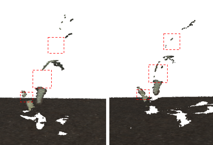
Figure 5: Reconstruction outcome from the 1-plant case. Left: Circle (Baseline). Right: GP-EI (Mattern $\nu$=2.5).

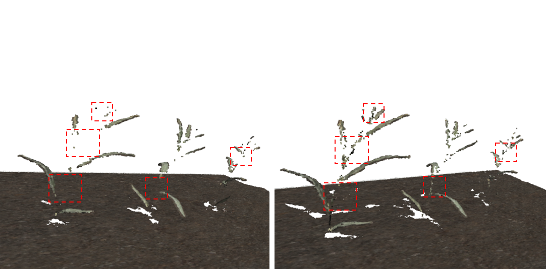
Figure 6: Reconstruction outcome from the 3-plants case. Left: Circle (Baseline). Right: GP-EI (RBF).

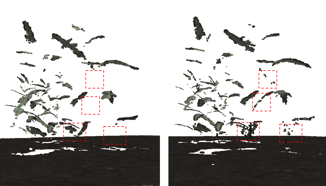
Figure 7: Reconstruction outcome from the 9-plants case. Left: Circle (Baseline). Right: GP-EI (RBF).

V Experiments

V-A Implementation Details

In our experimental setup and evaluation, we used the PyRender software [30] for the photo-realistic scene creation and the image rendering process. We considered three different environmental scenarios with 1-plant, 3-plants (row), and 9-plants (rectangle) as illustrated in Figs. 3(a), 3(b), and 3(c) respectively. The data used to create the simulated scenes were real-world reconstructions from artificial corn plants. Each plant was given a random rotation around its vertical axis and a scale within 10$\%$ of the original size. To emulate different realizations of the noise, we draw a sample $n\sim\pazocal{N}(n;0,0.005)$, and by starting from the lower levels of the plants, we gradually increased the noise value to the upper levels. This created a uniform movement of the plants, that could potentially simulate noise disturbances from the wind. It is worth noticing that our formulation can model and work on any type of noise, and the motion noise used here is just for demonstration purposes. The 3D reconstruction process was conducted with COLMAP [31, 32] using the default settings. For the RGB camera parameters, we set the $FoV=\frac{\pi}{2}$, $\theta_{match}=\frac{\pi}{4}$, and the rendering resolution at $2000\crossproduct 1500$. The number of cameras $N$ used for the reconstruction process was the minimum possible for each one of the three cases to demonstrate the benefits of regenerating 3D areas of interest in noisy environments with a very small budget. This minimum number of cameras was determined experimentally since, with fewer cameras, COLMAP was unable to offer a reconstruction. Specifically, $N$ is set to $N=4,6,6$ for the 1-plant, 3-plants and 9-plants cases respectively. As a baseline, we implemented a standard circular camera formation widely used as a brute-force approach for comparison in 3D reconstruction tasks; see e.g., [1].

To optimize the black-box reward function $\tilde{r}(\cdot)$, a BO framework was employed that adopts a GP-based surrogate model utilizing (i) a radial basis function (RBF) kernel, (ii) an RBF kernel with automatic relevance determination (henceforth abbreviated as ‘ARD’), (iii) a Matern kernel with parameter $\nu=2.5$ or (iv) a Matern kernel with parameter $\nu=1.5$. The AF used for the acquisition of new input points (i.e., camera position in the 3D space) is EI (c.f. Eqn. (12)). In all cases, 50 randomly selected input-output evaluation pairs were used for training the GP model, and 200 iterations were considered in the BO process. The kernel parameters along with the noise variance $\sigma_{n}^{2}$ were obtained by maximizing the marginal log-likelihood using the 50 initial training data, via GPytorch [33] and Botorch [34] packages.

In order to provide a fair comparison, the proposed method was compared with the baseline both quantitatively and qualitatively. The reported results in our three environmental cases consider five different noise realizations.

V-B Quantitative Evaluation

Initially, the performance of the proposed approach in optimizing the reward function $\tilde{r}(\cdot)$ is evaluated using the simple regret (SR) metric, which at iteration $t$ is expressed as

$$SR(t):=\tilde{r}(\mathbf{z}^{*})-\max_{\tau\in\{1,\ldots,t\}}\tilde{r}(\mathbf{z}_{\tau}).$$ (13)

Fig. 4 illustrates the SR performance of all competing approaches for the (a) 1-plant, (b) 3-plants, and (c) 9-plants cases, where the optimal value $\tilde{r}(\mathbf{z}^{*})=1$ in Eqn. (13) represents the maximum reward function value. For a fair comparison, the baseline SR value is equal to the best-performing one of 50 different circular camera placements. It is evident that all GP-EI approaches with different kernel functions consistently outperform the baseline after 90 iterations of the BO process in all cases. This showcases the significance of their benefits in balancing well the exploitation and exploration of the search space.

Upon obtaining the camera placement vector $\mathbf{z}$ that maximizes the $\tilde{r}(\cdot)$ function, the reconstruction quality was quantitatively assessed using as metric the absolute error of the depth images. The ground truth depth maps from each camera were provided by the PyRender tool. Table I depicts the average depth error along with the standard deviation of all approaches for five distinct noise realizations. It can be clearly seen that all advocated GP-EI approaches enjoy lower average absolute error compared to the baseline, with most of them achieving substantially improved 3D reconstruction quality performance. This corroborates the effectiveness of the proposed GP-EI approaches in selecting appropriate camera placements that provide sufficient information to accurately reconstruct areas of interest, even with a limited budget of available cameras. To further demonstrate the merits of the proposed approach, we present a number of qualitative experimental results as an alternative assessment of the 3D reconstruction.

V-C Qualitative Evaluation

Following the good performance of our method in the quantitative evaluation, our qualitative results in this subsection will further support the significance of our approach. Specifically, Figs. 5, 6, and 7 illustrate the 3D reconstructions in the form of point clouds for different noise realizations in all cases. In these figures, we highlight with red rectangle, a number of examples of the plant areas with noticeable improvements. In the first two scenarios (Figs. 5 and 6), our method can satisfactorily reconstruct the stem part of the plants, in contrast to the baseline that fails to capture any part of the stem. The last scenario considering 9-plants is more challenging due to the rectangle formation of the plants. Specifically, there are occlusion phenomena that are hard to address with a small number of cameras. Nevertheless, our proposed method can achieve significantly better reconstructions in this challenging case, as can be clearly seen in Fig. 7.

It is worth noticing that as expected, the reconstructions of all environmental cases are not fully aligned with the real environments due to the small number of cameras used, which may confine the visual information; refer also to Remark 2. The aim of this work is to corroborate the ability of the advocated method in accurately reconstructing noisy areas of interest even with a very small number of images at hand.

VI Conclusion

This paper focuses on the view planning problem of optimally placing a given set of cameras in the 3D space, so that to obtain sufficient visual information and accurately reconstruct a 3D area of interest. Unlike existing approaches in the literature, this work is the first to incorporate the existing noise of the environment in the VP problem without knowledge of the analytic noise expression. To optimize the so-termed reward function that gives an estimate of the reconstruction quality and whose closed-form expression is unknown due to the embodied noise, Bayesian optimization techniques are utilized. The latter provides assistance in effectively optimizing the black-box reward function in a sample-efficient manner. While most existing VP approaches entail discretizing the search space, the proposed approach hinges on a continuous optimization problem where any position belonging to the entire space can be explored. Numerical tests on noisy agricultural settings demonstrate the efficacy of the novel approach in accurately reconstructing 3D areas with only a small budget of available cameras.

Future directions include theoretical and robustness analysis of the proposed method, and its assessment on real-world agricultural environments. Further environmental scenarios can additionally be considered, with application to forest and fire monitoring or urban surveillance.

VII Acknowledgements

This work is supported by the Minnesota Robotics Institute (MnRI) and the National Science Foundation through grants #CNS-1439728, #CNS-1531330, and #CNS-1939033. USDA/NIFA has also supported this work through the grants 2020-67021-30755 and 2023-67021-39829. The work of Konstantinos D. Polyzos was also supported by the Onassis Foundation Scholarship.

References

- [1] A. Bacharis, H. J. Nelson, and N. Papanikolopoulos, “View planning using discrete optimization for 3d reconstruction of row crops,” in 2022 IEEE/RSJ International Conference on Intelligent Robots and Systems (IROS). IEEE, 2022, pp. 9195–9201.
- [2] H. J. Nelson, C. E. Smith, A. Bacharis, and N. P. Papanikolopoulos, “Robust plant localization and phenotyping in dense 3d point clouds for precision agriculture,” in 2023 IEEE International Conference on Robotics and Automation (ICRA). IEEE, 2023, pp. 9615–9621.
- [3] C. Peng and V. Isler, “View selection with geometric uncertainty modeling,” arXiv preprint arXiv:1704.00085, 2017.
- [4] P. Roy and V. Isler, “Active view planning for counting apples in orchards,” in 2017 IEEE/RSJ International Conference on Intelligent Robots and Systems (IROS). IEEE, 2017, pp. 6027–6032.
- [5] E. Vidal, N. Palomeras, K. Istenič, N. Gracias, and M. Carreras, “Multisensor online 3d view planning for autonomous underwater exploration,” Journal of Field Robotics, vol. 37, no. 6, pp. 1123–1147, 2020.
- [6] W. Jing, J. Polden, P. Y. Tao, W. Lin, and K. Shimada, “View planning for 3d shape reconstruction of buildings with unmanned aerial vehicles,” in 2016 14th International Conference on Control, Automation, Robotics and Vision (ICARCV). IEEE, 2016, pp. 1–6.
- [7] N. Smith, N. Moehrle, M. Goesele, and W. Heidrich, “Aerial path planning for urban scene reconstruction: A continuous optimization method and benchmark,” ACM Trans. Graph., vol. 37, no. 6, dec 2018. [Online]. Available: https://doi.org/10.1145/3272127.3275010
- [8] K. A. Tarabanis, P. K. Allen, and R. Y. Tsai, “A survey of sensor planning in computer vision,” IEEE transactions on Robotics and Automation, vol. 11, no. 1, pp. 86–104, 1995.
- [9] G. H. Tarbox and S. N. Gottschlich, “Planning for complete sensor coverage in inspection,” Computer vision and image understanding, vol. 61, no. 1, pp. 84–111, 1995.
- [10] C. Peng and V. Isler, “Adaptive view planning for aerial 3d reconstruction,” in 2019 International Conference on Robotics and Automation (ICRA). IEEE, 2019, pp. 2981–2987.
- [11] S. Pan, H. Hu, and H. Wei, “Scvp: Learning one-shot view planning via set covering for unknown object reconstruction,” IEEE Robotics and Automation Letters, vol. 7, no. 2, pp. 1463–1470, 2022.
- [12] B. Shahriari, K. Swersky, Z. Wang, R. P. Adams, and N. De Freitas, “Taking the human out of the loop: A review of Bayesian optimization,” Proc. IEEE, vol. 104, no. 1, pp. 148–175, 2015.
- [13] J. Snoek, H. Larochelle, and R. P. Adams, “Practical Bayesian optimization of machine learning algorithms,” Neural Information Processing Systems, vol. 25, 2012.
- [14] K. Korovina, S. Xu, K. Kandasamy, W. Neiswanger, B. Poczos, J. Schneider, and E. Xing, “Chembo: Bayesian optimization of small organic molecules with synthesizable recommendations,” International Conference on Artificial Intelligence and Statistics, pp. 3393–3403, 2020.
- [15] Z. Wang and S. Jegelka, “Max-value entropy search for efficient Bayesian optimization,” International Conference on Machine Learning, pp. 3627–3635, 2017.
- [16] A. Cully, J. Clune, D. Tarapore, and J.-B. Mouret, “Robots that can adapt like animals,” Nature, vol. 521, no. 7553, pp. 503–507, 2015.
- [17] R. Marchant and F. Ramos, “Bayesian optimisation for informative continuous path planning,” in International Conference on Robotics and Automation, 2014, pp. 6136–6143.
- [18] J. I. Vasquez-Gomez, L. E. Sucar, and R. Murrieta-Cid, “View planning for 3d object reconstruction with a mobile manipulator robot,” in 2014 IEEE/RSJ International Conference on Intelligent Robots and Systems. IEEE, 2014, pp. 4227–4233.
- [19] S. Pan, H. Hu, H. Wei, N. Dengler, T. Zaenker, and M. Bennewitz, “One-shot view planning for fast and complete unknown object reconstruction,” arXiv preprint arXiv:2304.00910, 2023.
- [20] C. E. Rasmussen and C. K. Williams, Gaussian processes for machine learning. MIT press Cambridge, MA, 2006.
- [21] Q. Lu, K. D. Polyzos, B. Li, and G. B. Giannakis, “Surrogate modeling for bayesian optimization beyond a single gaussian process,” IEEE Transactions on Pattern Analysis and Machine Intelligence, vol. 45, no. 9, pp. 11 283–11 296, 2023.
- [22] K. D. Polyzos, Q. Lu, and G. B. Giannakis, “Bayesian optimization with ensemble learning models and adaptive expected improvement,” in IEEE International Conference on Acoustics, Speech and Signal Processing (ICASSP). IEEE, 2023.
- [23] D. Nguyen, S. Gupta, S. Rana, A. Shilton, and S. Venkatesh, “Bayesian optimization for categorical and category-specific continuous inputs,” AAAI Conference on Artificial Intelligence, vol. 34, no. 04, pp. 5256–5263, 2020.
- [24] S. Gopakumar, S. Gupta, S. Rana, V. Nguyen, and S. Venkatesh, “Algorithmic assurance: An active approach to algorithmic testing using Bayesian optimisation,” Neural Information Processing Systems, pp. 5470–5478, 2018.
- [25] K. D. Polyzos, Q. Lu, and G. B. Giannakis, “Weighted ensembles for active learning with adaptivity,” arXiv:2206.05009, 2022.
- [26] W. R. Thompson, “On the likelihood that one unknown probability exceeds another in view of the evidence of two samples,” Biometrika, vol. 25, no. 3/4, pp. 285–294, 1933.
- [27] D. R. Jones, M. Schonlau, and W. J. Welch, “Efficient global optimization of expensive black-box functions,” Journal of Global optimization, vol. 13, no. 4, pp. 455–492, 1998.
- [28] N. Srinivas, A. Krause, S. Kakade, and M. Seeger, “Gaussian process optimization in the bandit setting: No regret and experimental design,” in International Conference on Machine Learning, 2010.
- [29] P. I. Frazier, “A tutorial on Bayesian optimization,” arXiv preprint arXiv:1807.02811, 2018.
- [30] M. Matl, “Pyrender,” https://github.com/mmatl/pyrender, 2019.
- [31] J. L. Schönberger and J.-M. Frahm, “Structure-from-motion revisited,” in Conference on Computer Vision and Pattern Recognition (CVPR), 2016.
- [32] J. L. Schönberger, E. Zheng, M. Pollefeys, and J.-M. Frahm, “Pixelwise view selection for unstructured multi-view stereo,” in European Conference on Computer Vision (ECCV), 2016.
- [33] J. R. Gardner, G. Pleiss, D. Bindel, K. Q. Weinberger, and A. G. Wilson, “Gpytorch: Blackbox matrix-matrix gaussian process inference with gpu acceleration,” in Advances in Neural Information Processing Systems, 2018.
- [34] M. Balandat, B. Karrer, D. R. Jiang, S. Daulton, B. Letham, A. G. Wilson, and E. Bakshy, “BoTorch: A Framework for Efficient Monte-Carlo Bayesian Optimization,” in Advances in Neural Information Processing Systems 33, 2020. [Online]. Available: http://arxiv.org/abs/1910.06403