Coarse-graining and criticality in the human connectome

Abstract

In the face of the stupefying complexity of the human brain, network analysis is a most useful tool that allows one to greatly simplify the problem, typically by approximating the billions of neurons comprising the brain by means of a coarse-grained picture with a practicable number of nodes. But even such relatively small and coarse networks, such as the human connectome with its 100-1000 nodes, may present challenges for some computationally demanding analyses that are incapable of handling networks with more than a handful of nodes. With such applications in mind, we set out to further coarse-grain the human connectome by taking a modularity-based approach, the goal being to produce a network of a relatively small number of modules. We applied this approach to study critical phenomena in the brain; we formulated a hypothesis based on the coarse-grained networks in the context of criticality in the Wilson-Cowan and Ising models, and we verified the hypothesis, which connected a transition value of the former with the critical temperature of the latter, using the original networks. We found that the qualitative behavior of the coarse-grained networks reflected that of the original networks, albeit to a less pronounced extent. This, in principle, allows for the drawing of similar qualitative conclusions by analysing the smaller networks, which opens the door for studying the human connectome in contexts typically regarded as computationally intractable, such Integrated Information Theory and quantum models of the human brain.

I Introduction

The sheer complexity of the human brain constitutes a formidable obstacle to the construction of a complete theory of its workings. Network analysis Sporns (2003) serves as an exceedingly powerful tool that breaks down the problem by modeling the brain, with its billions of neurons, as a network comprising a much more manageable number of nodes. In this simplified picture, it becomes computationally feasible to conduct graph-theoretical investigations Zalesky et al. (2010); Bassett and Sporns (2017); Bullmore and Sporns (2009) from which a great deal of neuroscientific insight may be extracted.
One such example is the structural human connectome, which is a comprehensive map of neural connections in the brain that may be constructed at different degrees of granularity. It typically comprises a number of nodes of $\sim 100$, with some other atlases containing as many as a few hundred Rosen and Halgren (2021). There, each node represents a large collection of neurons, such as an anatomical brain region. The structural connectivity matrix of such a network may be extracted from data obtained through non-invasive neuroimaging techniques such as diffusion tensor imaging Jbabdi et al. (2015); Shi and Toga (2017); Hagmann et al. (2010). Patterns of functional activity may also be observed through functional magnetic resonance imaging (fMRI) scans, enabling the construction of the functional human connectome, in which the edges between nodes represent statistical correlations based on similarity measures between neuronal components Raichle (2009); Hagmann et al. (2010); Lang et al. (2012). These functional networks may serve as graphical representations of the dynamical patterns that emerge spontaneously in the brain, as well as those which manifest themselves during the performance of tasks Eguíluz et al. (2005); Heuvel et al. (2008).
But even such relatively small and coarse networks are intractable in the context of certain demanding approaches where, for instance, computational costs grow exponentially or super-exponentially with the number of nodes. One such example is the integrated information theory (IIT) of consciousness, which is a framework that seeks to quantify consciousness by introducing the quantity $\Phi$, a number that characterizes the extent to which a dynamical system generates information that is irreducible to the sum of its parts (see Ref. Oizumi et al., 2014 for a comprehensive review). IIT is often regarded as an alternative hypothesis to the other prominent theory of consciousness, global workspace theory Baars (2005). The cost of computing $\Phi$ explodes combinatorially as a function of the number of nodes, rendering the problem insurmountable for systems comprising more than a handful of nodes.
Furthermore, recent years have seen a rising interest in quantum effects in the brain Adams and Petruccione (2020); Smith et al. (2021); Zadeh-Haghighi and Simon (2021), and in theories which attempt to make connections between quantum mechanics and consciousness Hameroff and Penrose (2014); Fisher (2014). Consequently, models of the brain which can incorporate quantum phenomena are of ever-growing interest. Simulations of such quantum models of the brain on a classical computer, however, are computationally expensive in a manner which grows exponentially with the number of nodes. Therefore, to grapple with either of these applications (IIT and quantum models of the brain) in the context of the human connectome, it is essential to employ a coarse-graining approach to reduce the size of the human connectome by at least an order of magnitude.
To that end we set out to identify a suitable coarse-graining procedure. There is a number of approaches proposed in the literature for detecting communities in networks, such as ones based on centrality indices Girvan and Newman (2002) and spectral methods Capocci et al. (2005). We employ the algorithm proposed in Blondel et al. (2008), which is a simple and efficient algorithm to partition the networks into communities by maximizing the modularity of the network.
After applying this approach to the human connectome, we investigate the extent to which the resulting coarse-grained networks resemble the original networks. As a sanity check, we start by verifying that the global structures of the simplified networks resemble those of the original ones. Next, we turn our attention to models of the dynamical behavior of the brain, and study the preservation of such behavior in going from the large networks to the small ones.
The first model we consider is that of Wilson-Cowan oscillators Wilson and Cowan (1972), a biologically motivated description of the dynamics of neuronal populations. In the form of choice, the model contains but one free parameter, referred to as $c_{5}$, which may be varied to control the dynamical state of the network. A salient feature of this model is the presence of a critical point; upon exceeding a certain value of $c_{5}$, typically denoted as $c_{5}^{T}$, the system transitions from a globally inactive state into a globally excited state in which a preponderance of oscillatory activity manifests itself in a great number of brain regions. $c_{5}^{T}$, which may be regarded as a given brain network’s capacity for global excitation, has been observed to vary across individual subjects Muldoon et al. (2016) and to correlate with a number of cognitive measures Bansal et al. (2018a). It has also been demonstrated that biological networks tend to be more easily excitable than randomized networks, despite being less strongly connected Kora et al. (2023).
Another popular framework that is utilized in this context is the Ising model, by virtue of being one of the simplest models with site-dependent binary variables, and only one parameter, i.e., the temperature of the thermal bath. In one early study Fraiman et al. (2009), it was found that brain networks derived from the fMRI BOLD (blood-oxygen-level dependent) signals were statistically equivalent to networks derived from the 2D Ising model at the critical temperature. In another Marinazzo et al. (2014), the Ising model was studied with variable couplings that were defined according to the anatomical connectivity matrix, and total information transfer was found to be maximized at the critical temperature. Both of these investigations lend support to the so-called critical brain hypothesis Bak et al. (1988); Massobrio et al. (2015); Korchinski et al. (2021), which conjectures that brain dynamics take place at the so-called edge of chaos, i.e., the critical boundary between stability and disorder.
An Ising model with variable couplings between the spin-sites is often referred to as a generalized Ising model (GIM). Such models have been the subject of a number of recent studies that seek to model the spontaneous activity of the brain given the underlying anatomical structure. In Ref. Abeyasinghe et al., 2018, for instance, the couplings in the GIM were defined to be proportional to the number of fibres connecting each pair of brain regions, and the thermodynamics and critical properties of this model were calculated in a Monte Carlo (MC) simulation and compared to those of the 2D Ising model. Correlation functions may also be computed by defining the notion of distance as the reciprocal of the connectivity. A similar study Abeyasinghe et al. (2020) was performed using different sets of anatomical structural data, including those obtained from patients with severe brain injuries and disorders of consciousness (DOC). This enabled the investigation of the relationship between the critical properties of the model and consciousness, and it was observed that subjects suffering from DOC tended to exhibit higher critical temperatures.
In this work, we evaluate the soundness of the coarse-graining approach using the Wilson-Cowan model by applying it to both the coarse-grained and original networks, and measuring the extent to which the behavior is preserved between them. After verifying that the small networks are adequately representative of the large ones in this dynamical context, we seek to make connections between the transition that takes place in the in the model of Wilson-Cowan oscillators and criticality in the Ising model. This allows us to hypothesize, based on the coarse-grained networks, a relationship between the transition value of the Wilson-Cowan model $c_{5}^{T}$ and the critical temperature of the Ising model $T_{c}$, thereby introducing the former to the aforementioned association with DOC that was previously observed for the latter (in Ref. Abeyasinghe et al., 2020). We finally verify that hypothesis by the aid of the original networks.
The remainder of this paper is organized as follows: in section II we describe our dynamical models and methodology for data extraction and coarse-graining. We present and discuss our results in section III, and finally outline our conclusions in section IV.

II Materials and Methods

II.1 Wilson-Cowan model

We are interested in the form of the Wilson-Cowan model used in Ref. Bansal et al. (2018a) (but in the absence of an external stimulation), wherein all neurological processes of interest are assumed to be governed by the interaction between excitatory and inhibitory cells. Furthermore, each subpopulation of such cells at every brain region is modeled by a single variable; we define $E_{i}$ and $I_{i}$ as the respective fractions of excitatory and inhibitory cells firing per unit time in region $i$. Thus the model reads

$$\tau\frac{dE_{i}}{dt}=-E_{i}(t)+(S_{E_{m}}-E_{i}(t))\times\\ S_{E}\left(c_{1}E_{i}(t)-c_{2}I_{i}(t)+c_{5}\sum_{j}J_{ij}E_{j}(t-\tau_{d}^{ij})\right)\\ +\sigma w_{i}(t)$$ (1)

and

$$\tau\frac{dI_{i}}{dt}=-I_{i}(t)+(S_{I_{m}}-I_{i}(t))\times\\ S_{I}\left(c_{3}E_{i}(t)-c_{4}I_{i}(t)+c_{6}\sum_{j}J_{ij}I_{j}(t-\tau_{d}^{ij})\right)\\ +\sigma v_{i}(t)$$ (2)

where $S_{E,I}(x)$ are sigmoid functions given by

$$S_{E,I}(x)=\frac{1}{1+e^{-a_{E,I}(x-\theta_{E,I})}}-\frac{1}{1+e^{a_{E,I}\theta_{E,I}}}$$ (3)

$S_{E_{m},I_{m}}$ are the maxima thereof, and the constants $a_{E,I}$ and $\theta_{E,I}$ respectively determine the value and position of maximum slope. $J_{ij}$ are the elements of the structural connectivity matrices. On account of the physical distance $d_{ij}$ between two brain regions, there exists a communication delay $\tau_{d}^{ij}=d_{ij}/v_{d}$, where $v_{d}=10$ m/s is a typical estimate of the signal transmission velocity (see, for instance, Ref. Waxman and Bennett, 1972). Finally, a normal distribution of noise of strength $\sigma$ is injected into the system by means of the functions $w_{i}(t)$ and $v_{i}(t)$. This form of the model is standard in the literature Muldoon et al. (2016); Bansal et al. (2018a, b), but in principle the model may be generalized to incorporate, for instance, couplings between opposing types of cells.
We utilized a second order Runge-Kutta solver with a sufficiently fine timestep, such that the results were independent of the size thereof. For each individual subject, the value of $c_{5}^{T}$ was estimated by simulating the model at multiple values of $c_{5}$ and observing the point at which the transition took place.

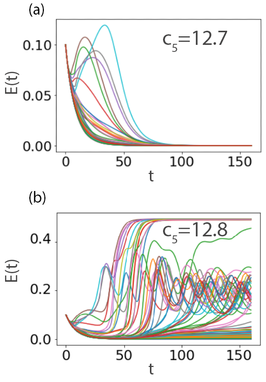
Figure 1: An example of the Wilson-Cowan transition: the dynamics of the proportion of excitatory cells firing per unit time, for a certain brain network, at $c_{5}=12.7$ (a) and $c_{5}=12.8$ (b). Each line corresponds to a brain region.

The oscillators were always initialized in the state with $E=I=0.1$. The parameters defined above were fixed at $\sigma=10^{-5}$, $c_{1}=16$, $c_{2}=12$, $c_{3}=15$, $c_{4}=3$, $a_{E}=1.3$, $a_{I}=2$, $\theta_{E}=4$, $\theta_{I}=3.7$, and $\tau=8$ as prescribed in the literature Muldoon et al. (2016); Bansal et al. (2018a). At this choice of the parameters, the oscillators may be found in one of three states: a low fixed point, a high fixed point, and an oscillatory limit cycle in-between Muldoon et al. (2016). A biological network typically exhibits an abrupt transition into a globally excited state, i.e., from a state where all initial activity rapidly dwindles down to the lower fixed point, to one where a substantial proportion of oscillators are activated into the limit cycle or the high fixed point. Such a transition may be accomplished by ramping up the global coupling parameter $c_{5}$, and crossing a critical value thereof, at which the state of the system abruptly changes, as illustrated in Fig. 1. The transition value, typically referred to as $c_{5}^{T}$, will henceforth be referred to as simply $c_{5}$ for ease of notation. As mentioned above, this value is unique for each subject for a given choice of parameters and initial conditions ana .

II.2 Generalized Ising model

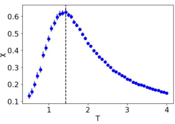
Figure 2: An example of the magnetic susceptibility as a function of temperature for a given network of Ising spins. The critical temperature is estimated by locating the peak (black dashed line). Bars correspond to statistical errors, which may be used to infer the uncertainty on the critical temperature by identifying the range of temperature at which the statistical errors overlap with the maximum.

We consider a system comprising $N$ lattice sites, each with spin $s_{i}=\pm 1$ along the z-direction. In the absence of an external magnetic field, the energy of a configuration $s=\{s_{i}\}$ is given by the pairwise interaction

$$H(s)=-\sum_{i<j}J_{ij}s_{i}s_{j}$$ (4)

where the sum runs over all pairs of particles. This system is more general than the Ising model, in the sense that a) the sum is not restricted to nearest neighbours, and b) the coupling strength $J_{ij}$ of the interaction between two lattice sites is arbitrarily non-uniform. Thus it is referred to as the generalized Ising model.
Clearly, the physics of this model at any given temperature is completely determined by the coupling strength matrix $\bf J$. which may be chosen to describe an arbitrary model for the interaction between an arbitrary number of spin sites in an arbitrary number of dimensions.
As alluded to above, the GIM may serve as a dynamical model of the human brain through the following mapping: each spin site represents a brain region, and the corresponding value of $s_{i}$ represents the value of a binary variable associated with that brain region, such as the BOLD signal. The coupling strength matrix $J_{ij}$ is mapped onto the structural connectome by, for instance, being made proportional to the number of fibres connecting two regions.
We perform simulations of the system described by eq. 4, at each temperature, by means of the Metropolis Monte Carlo algorithm Metropolis et al. (1953) that is the same regardless of the value of $\bf J$. The details of the simulation are standard; we start from a random spin configuration, and sample new configurations with a probability proportional to the corresponding Boltzmann weight, exp$(-E(\{s_{i}\})/T)$. First, a sufficient number of MC steps is performed to ensure convergence towards thermodynamic equilibrium (a single MC step is defined to be a number of iterations such that, on average, each of the spin sites is subject to one flipping attempt). Once that is achieved, thermal expectation values of the quantities of interest are computed as statistical averages over configurations separated by an appropriate number of MC steps. The magnetization, for instance, is given by

$$m=\frac{1}{N}\sum_{i=1}^{N}s_{i}$$ (5)

and the magnetic susceptibility, defined as $\frac{\partial m}{\partial h}\Bigr{\rvert}_{h\to 0}$, is given by

$$\chi=\frac{N}{T}\left(\langle m^{2}\rangle-\langle m\rangle^{2}\right)$$ (6)

and the specific heat by

$$C=\frac{N}{T^{2}}\left(\langle e^{2}\rangle-\langle e\rangle^{2}\right)$$ (7)

where $e=E/N$, the total energy of the system per particle. One may study the phase transition by simulating the system at different temperatures, plotting those quantities thereagainst, and inferring the critical temperature by identifying the peak in the magnetic susceptibility (see Fig. 2). Naturally, the caveats here are 1) that the smaller the network, the more prominent the finite-size effects; and 2) the existence of other methods to estimate the critical temperature.

II.3 Structural data and measures

We constrained the dynamical models outlined in subsections II.1 and II.2 by a set of undirected structural connectivity matrices extracted from imaging data, which we obtained from the 1200 subject cohort of the Human Connectome Project (HCP), a database containing neural data for thousands of subjects, of which we selected a sample for our calculations. On no particular basis did we choose from among the 1200 subjects; we merely selected the first subjects on the list, about whom no information was provided besides age and gender. Both pre-processed T1-weighted structural images and 3T dMRI images were used in our computational fibre tracking method. Python DIPY and NiBabel libraries were utilized to perform the streamline calculations using a constrained spherical deconvolution model and probabilistic fibre tracking functions, which are built in the libraries.
Each structural connectivity network emerging from this procedure belongs to an individual subject, and comprises 104 nodes, each node corresponding to a cortical or subcortical brain structure. A full list of those brain structures may be found in Table 1 in the Appendix. The networks were then normalized by dividing the strength of each connection by the sum of the volumes of its two nodes, as in earlier studies Muldoon et al. (2016); Bansal et al. (2018a).
As our first measure of global structure we calculate the global efficiency Stam and Reijneveld (2007), which measures the extent to which a graph is well-connected by computing the average inverse shortest distance between pairs of vertices. The expression reads

$$E_{glob}=\frac{1}{N(N-1)}\sum_{i\neq j}\frac{1}{s_{ij}}$$ (8)

where $N$ is the number of nodes, and $s_{ij}$ is the shortest distance between nodes $i$ and $j$ (not to be confused with the physical distance $d_{ij}$). We also compute the characteristic path length Stam and Reijneveld (2007), which is another (roughly anti-proportional) way of characterizing the well-connectedness of a graph, previously used Kora et al. (2023) in the context of the Wilson-Cowan model glo . It is computed as the average path length between all possible pairs of vertices:

$$L=\frac{1}{N(N-1)}\sum_{i,j\in N,i\neq j}s_{ij}$$ (9)

II.4 Coarse-graining algorithm

We employed a coarse-graining algorithm based on the method prescribed in Blondel et al. (2008) for detecting communities in networks. The goal is to partition a given network into the set of communities that maximizes the quantity known as the modularity, which quantifies the strength of the connections within communities relative to the strength of the connections between communities. In the cases of a weighted network with a connectivity matrix ${\bf J}$, this may be written as

$$Q=\frac{1}{2m}\sum_{i,j}\left[J_{ij}-\frac{d_{i}d_{j}}{2m}\right]\delta(c_{i},cj)$$ (10)

where $d_{i}$ is the degree centrality of node $i$, defined as $d_{i}=\sum_{i=1}^{N}J_{ij}$; $c_{i}$ is the community to which node $i$ belongs; $\delta(u,v)$ is a Kronecker delta, equaling 1 if u=v and 0 otherwise; and $m=\frac{1}{2}\sum_{ij}J_{ij}$.
The algorithm comprises a series of passes, each pass consisting of two phases. Phase one begins in a maximum entropy configuration with each node assigned to its own community, such that the number of communities is equal to the number of nodes. Next, each neighbouring node $j$ of node $i$ is considered, and we compute the gain in modularity on account of moving node $i$ into the community containing node $j$. Node $i$ is subsequently removed from the community to which it originally belonged, and placed into the community for which the gain in modularity is maximum (provided that gain is positive). All nodes in the network are subjected to this process sequentially and repeatedly, until the modularity may no longer be increased by any such moves, thereby reaching a local maximum and concluding phase one.
To evaluate the change in modularity arising from the moving of an isolated node $i$ into a community $C$, we make use of the computationally efficient expression given in Ref. Blondel et al. (2008), namely

$$\Delta Q=\left[\frac{\Sigma_{in}+k_{i,in}}{2m}-\left(\frac{\Sigma_{tot}+k_{i}}{2m}\right)^{2}\right]-\\ \left[\frac{\Sigma_{in}}{2m}-\left(\frac{\Sigma_{tot}}{2m}\right)^{2}-\left(\frac{k_{i}}{2m}\right)^{2}\right]$$ (11)

where $\Sigma_{in}$ is the sum of the weights within $C$, $\Sigma_{tot}$ is the sum of the weights incident to nodes in $C$, and $k_{i,in}$ is the sum of the weights from $i$ to nodes in $C$.
Phase two of the algorithm is concerned with the construction of a new network whose nodes are the communities obtained in phase one. In this new network, the link connecting two nodes is obtained by summing up the weights of the links between the the two communities which the two nodes represent. This obviously gives rise to self-loops, which may either be represented as self-interactions or ignored altogether. For the purposes of this work, we do not incorporate self-interactions, as the original networks did not contain anything of the sort. It is important to note that the weights of the non-self loop links are not renormalized at any step of the algorithm. We also compute the distances between nodes in the new network. Now that the nodes are no longer strictly correspondent to anatomical brain regions, a new definition of the distance is in order; we define the distance between two communities as the weighted mean of the distances between the nodes therein.
We arrive at the partitioning which maximizes the modularity by iterating the passes of the algorithm until no more increases to the modularity may be achieved.

III Results and Discussion

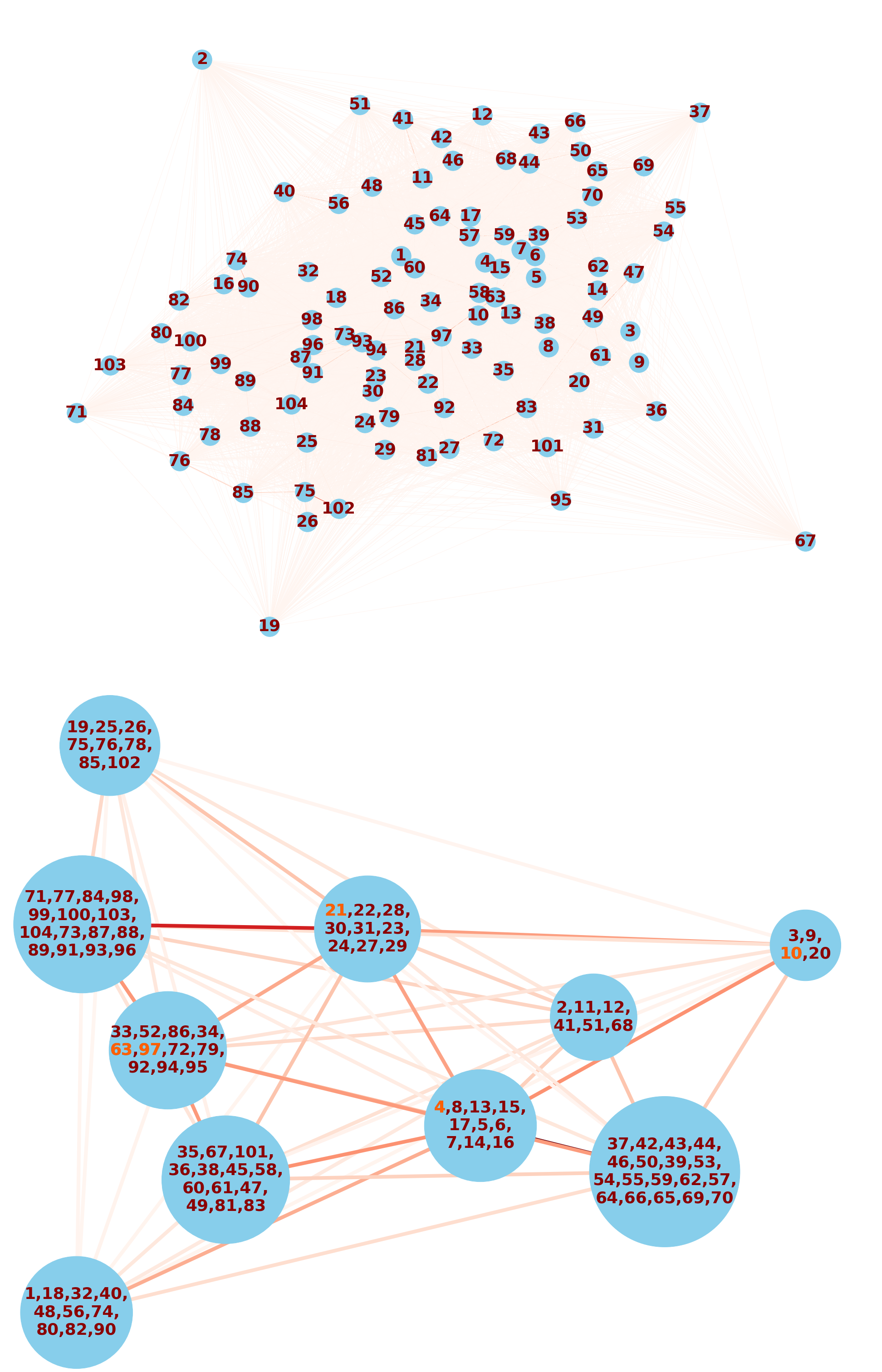
Figure 3: A visualization of the relationship between one brain network (top) and its coarse-grained counterpart (bottom). Numbers correspond to brain regions in accordance with the list given in Table 1 in the Appendix. The darkness of a given edge is proportional to its weight. The area of a given node in the coarse-grained network is proportional to the number of brain regions it contains. Highlighted numbers in the coarse-grained network correspond to the most salient brain regions according to Ref. Salhi et al. (2023)

.

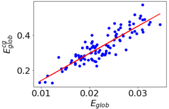
Figure 4: The global efficiency of the coarse-grained networks obtained vs. the global efficiency of the corresponding original networks. Each dot represents a different subject. The red line is a least-squares fit with $r^{2}=0.786$.

The outcome of applying the procedure outlined in subsection II.4 to the networks described in subsection II.3 is a reduction of any given 104-node network to one comprising 10-14 nodes, depending on the subject. One such network and its corresponding coarse-grained network are visualized in Fig. 3. Each number corresponds to a brain region as given by the list in Table 1. The most prominent brain regions, as reported by the centrality analyses conducted in Ref. Salhi et al. (2023), include the brainstem (10), and both sides of the superiorfrontal cortex (63 and 97) and thalamus (4 and 21), all of which regions are highlighted in orange.
We now investigate the degree to which these small networks are representative of the original networks from which they emerged. Henceforth, we attach to all variables relating to the maximally coarse-grained networks the superscript “$cg$”, e.g., $T_{c}^{cg}$ is the critical temperature of the coarse-grained networks.
We begin by looking at global structure. We computed the global efficiency, as defined in subsection II.3, for each subject’s network and the corresponding maximally coarse-grained network. The result of which computation is presented in Fig. 4, which shows a fairly strong ($r^{2}=0.879$) correlation between the global efficiencies of both types of network. This is an encouraging result, as it indicates that the original networks of 104 nodes are fairly well-represented by the networks of 10-14 nodes which emerged from our coarse-graining procedure.

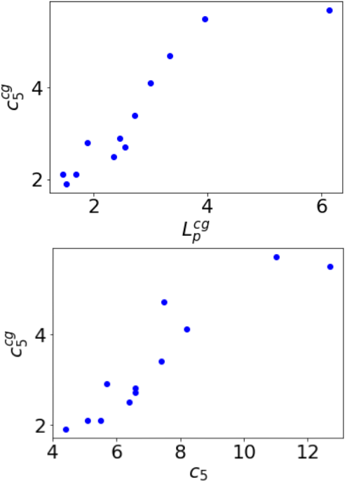
Figure 5: The transition value of $c_{5}$ for the coarse-grained networks against the (top) corresponding characteristic path length ($r^{2}=0.828$) and (bottom) transition value of $c_{5}$ for the corresponding original network ($r^{2}=0.859$).

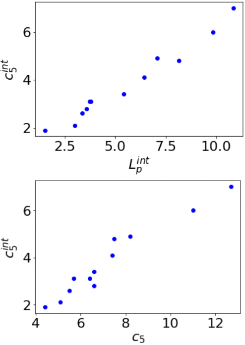
Figure 11: The same as Fig. 5, but for intermediately coarse-grained networks. Errors are small than symbol sizes. $r^{2}=0.970$ and $r^{2}=0.939$.

Emboldened by this finding, we turn our attention to dynamical behavior. We start by asking the question of whether we may arrive at similar conclusions to those of Ref. Kora et al., 2023, in which the full-sized networks were studied, by instead looking at the coarse-grained networks. We do so by implementing the Wilson-Cowan model on our small networks.
The first relationship we expect to see, based on the results of Ref. Kora et al., 2023, is a positive correlation between the transition value and the corresponding characteristic path length. This is an observation that the more well-connected a biological network is, the more global excitable it tends to be. Fig. 5 (top) shows the result of this investigation, which clearly assures us that this behavior is enjoyed by the coarse-grained networks as it is by the original ones. We also see in 5 (bottom) a substantial positive correlation $r^{2}=0.859$ between the the transition value for the small networks and the large ones, further validating the similarity between the two types of networks.
It must be noted here that such strong correlations are contingent on performing the coarse-graining procedure in the form prescribed in subsection II.4. We have experimented with some deviations from that prescription, which have invariably degraded the extent to which the behavior of the coarse-grained networks represented that of the original ones. For instance, this representation was slightly diminished when we tried taking the connectivity between modules to be the average of edge weights rather than their sum, as we show in Fig. 10 in the Appendix. The representation was also greatly diminished when we attempted to normalize the weights of the non-self loop links in the intermediate steps of the algorithm (to wit by dividing the weights of the links by the weight of the greatest link among them after each pass of the algorithm); the correlation between $c_{5}^{cg}$ and $c_{5}$ was completely lost, as well as that between the $E_{glob}^{cg}$ and $E_{glob}$. This breakdown suggests that the normalizing at intermediate steps leads to the erasure of important information as to the weights of the inter-module links with respect to the original networks. Indeed, when the prescription outlined above is adhered to, the behavior is consistent across multiple coarse-graining scales, as shown in Fig. 11 in the Appendix.

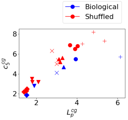
Figure 6: The transition value of $c_{5}$ for the coarse-grained networks against the corresponding characteristic path length, for both biological networks (blue) and shuffled networks (red). Symbol shapes corresponds to indivudal subjects.

The second conclusion drawn in Ref. Kora et al., 2023 is that randomized networks tend to be less globally excitable (i.e., higher value of $c_{5}$) than biological ones, despite being more well-connected (lower characteristic path length). This phenomenon is also observed for coarse-grained networks networks, albeit substantially less pronounced, as indicated in Fig. 6. We can clearly see that the red line (shuffled networks, generated by shuffling pairwise connectivities while preserving their distribution) invariably lies above the blue line (biological networks of the same subjects), but by a significantly smaller amount compared to the case of the original networks, as may be seen in Ref. Kora et al., 2023. This suggests that by studying the coarse-grained networks in lieu of the full-sized ones, one may derive qualitatively similar conclusions, but might fail to observe the full quantitative extent thereof. It may be argued that the red line is closer to the blue line in the coarse-grained networks, compared to the original ones, on account of the smaller effect of shuffling in smaller networks with respect to larger ones.
At this stage, it’s clear that the reduced networks produced from the coarse-graining procedure retain not only significant structural properties, but also a good deal of dynamical behavior. Thus we proceed to investigate the Ising model for the coarse-grained system, in the hopes that the conclusions we draw represent reality nearly as much as those directly drawn from the human connectome itself.

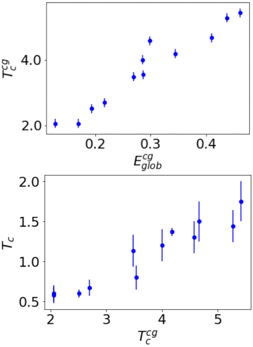
Figure 7: The Ising critical temperature as a function of global efficiency, for the coarse-grained networks ($r^{2}=0.930$) (top), and the correlation between the critical temperatures in the full and coarse-grained pictures ($r^{2}=0.917$) (bottom).

We begin by computing the Ising critical temperature, as described in subsection II.2 for a variety of coarse-grained networks, and investigating how it varies with the global efficiency introduced in subsection II.3. The advantage of simulating the Ising model on such small systems is that the simulations are rapid and efficient, and so the statistical errors of the thermal expectation values may be shrunk arbitrarily, allowing for an arbitrarily precise estimation of the critical temperature. The result of this is displayed in Fig. 7 (top), which shows a strong positive correlation ($r^{2}=0.930$), indicating that well-connected networks possess higher critical temperatures. As a sanity check, we compare the coarse-grained critical temperatures with those computed for the original networks in Fig. 7 (bottom), in order to verify that there is indeed a strong correlation, notwithstanding the size of the uncertainties on the critical temperature; they are inferred from the magnetic susceptibility data by estimating the range in which the peak is expected to lie in light of the statistical errors. In the case of the original networks, those statistical errors are substantial, they being the product of rather ponderous simulations in which the accumulation of statistics takes a long time.

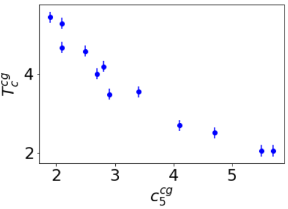
Figure 8: The Ising critical temperature as a function of the Wilson-Cowan transition value, for the coarse-grained networks ($r^{2}=0.918$)

.

Now that we have established that the behavior of the coarse-grained networks is fairly well-representative of the original ones, we are poised to use the coarse-grained networks to connect the two dynamical models and the two different senses of criticality therein. In Fig. 8, we plot the Ising critical temperature for the coarse-grained networks, $T_{c}^{cg}$, against the Wilson-Cowan transition value, $c_{5}^{cg}$. We clearly see a negative correlation between the two quantities, which is consistent with the findings presented in both Figs. 5 and 7, taken together with the fact that the characteristic path length and the global efficiency are opposing measures. The inverse relationship between $T_{c}$ and $c_{5}$ illustrated in Fig. 8 suggests that highly excitable brain networks (i.e., with low values of $c_{5}^{T}$, denoted as $c_{5}$), which is a property enjoyed by biological networks relative to randomized ones Kora et al. (2023), tend to possess higher critical temperatures. This here is a surprising result when considered with reference to one of the findings of Ref. Abeyasinghe et al., 2020, namely the association of a high Ising critical temperature with the presence of a disorder of consciousness. Naively, one might have expected randomized networks to exhibit behavior closer to DOC networks than to healthy ones, but here we have a set of observations that seem to suggest that when it comes to a network’s global excitability, shuffled networks possess the least, followed by biological networks (which observation may be directly seen in Fig. 6 and is presented and discussed in more detail in Ref. Kora et al., 2023), followed by the most excitable networks of all: DOC networks (which may be inferred from Fig. 8 in conjunction with the association of high $T_{c}$ with DOC reported in Ref. Abeyasinghe et al. (2020)).

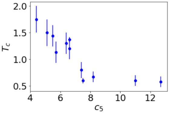
Figure 9: The Ising critical temperature a function of the Wilson-Cowan transition value for the original networks ($r^{2}=0.682$).

Finally, we may validate this conclusion drawn from the simplified networks, provided we are prepared to contend with the sluggishness of the Ising simulations on the unsimplified networks, and with substantial uncertainties arising from substantial statistical errors. The results, shown in Fig. 9, are certainly encouraging; the relationship between the Ising critical temperature and the Wilson-Cowan transition value bears a good deal of resemblance to the coarse-grained case, notwithstanding the disparity in the sizes of the uncertainties. This lends further credence to the belief that the coarse-graining procedure yields networks that are both significantly simpler to work with and adequately representative of the original networks, and that one may ascribe considerable validity to hypotheses developed based on the coarse-grained networks.

IV Conclusions

Inspired by the idea that the human connectome itself is indeed a coarse-grained picture, we set out to effect further coarse-graining in an effort to render the networks small enough for analyses of exceeding computational cost. To that end, we employed a modularization approach that allowed us to reduce the 104-node networks to networks comprising but 10-14 nodes.
These coarse-grained networks were found to be adequately representative of the original networks in both structural and dynamical contexts, provided that the coarse-graining procedure is carried out in a certain form. Encouraged by this, we used the small networks to formulate a hypothesis concerning the relationship between two dynamical models: Wilson-Cowan and Ising. Finally, we used the unsimplified networks to verify our hypothesis, which suggests that our approach may be generally viable, and emboldens us to pursue further applications.
Such applications include Integrated Information Theory and theories of the quantum brain, where the computational complexity is exponential or super-exponential in the number of nodes. The human connectome in its traditional form typically comprises 100-1000 nodes, which is far too large a number for any such applications. Fortunately, our findings here indicate that conclusions drawn based on coarse-grained networks may be valid enough, which provides a path to more explicit analyses in the aforementioned contexts.

V Acknowledgments

This work was supported by the Natural Sciences and Engineering Research Council (NSERC) of Canada through its NSERC Discovery Grant Program, the Alberta Major Innovation Fund, National Research Council through its Applied Quantum Computing Challenge Program, and Quantum City. We would also like to thank Joern Davidsen for the useful discussions and feedback, and Salma Salhi for providing the structrual data. Additionally, we thank the HCP for providing access to their data.

Data Availability Statement

The data used in this project was provided by the Human Connectome Project (HCP; Principal Investigators: Bruce Rosen, M.D., Ph.D., Arthur W. Toga, Ph.D., Van J. Weeden, MD). HCP funding was provided by the National Institute of Dental and Craniofacial Research (NIDCR), the National Institute of Mental Health (NIMH), and the National Institute of Neurological Disorders and Stroke (NINDS). HCP data are disseminated by the Laboratory of Neuro Imaging at the University of Southern California. Structural and diffusion MRI images from the HCP, as well as lists of extracted structures, bvals, and bvecs, were all used to process the data in our Python program. All subjects are part of the “WU-Minn HCP Data - 1200 Subjects” dataset. A complete list of subject names is available upon request. All scripts used to generate the connectomes are available on our Github repository found at https://github.com/SalmaSalhi7/Structural-Connectome-Project.

VI Appendix

VI.1 List of Brain regions

Table 1: A full list of the 104 brain structures.

ID	Structure
1	Left-Lateral-Ventricle
2	Left-Inf-Lat-Vent
3	Left-Cerebellum-Cortex
4	Left-Thalamus-Proper
5	Left-Caudate
6	Left-Putamen
7	Left-Pallidum
8	3rd-Ventricle
9	4th-Ventricle
10	Brain-Stem
11	Left-Hippocampus
12	Left-Amygdala
13	CSF
14	Left-Accumbens-area
15	Left-VentralDC
16	Left-vessel
17	Left-choroid-plexus
18	Right-Lateral-Ventricle
19	Right-Inf-Lat-Vent
20	Right-Cerebellum-Cortex
21	Right-Thalamus-Proper
22	Right-Caudate
23	Right-Putamen
24	Right-Pallidum
25	Right-Hippocampus
26	Right-Amygdala
27	Right-Accumbens-area
28	Right-VentralDC
29	Right-vessel
30	Right-choroid-plexus
31	Optic-Chiasm
32	CC_Posterior
33	CC_Mid_Posterior
34	CC_Central
35	CC_Mid_Anterior
36	CC_Anterior
37	ctx-lh-bankssts
38	ctx-lh-caudalanteriorcingulate
39	ctx-lh-caudalmiddlefrontal
40	ctx-lh-cuneus
41	ctx-lh-entorhinal
42	ctx-lh-fusiform
43	ctx-lh-inferiorparietal
44	ctx-lh-inferiortemporal
45	ctx-lh-isthmuscingulate
46	ctx-lh-lateraloccipital
47	ctx-lh-lateralorbitofrontal
48	ctx-lh-lingual
49	ctx-lh-medialorbitofrontal
50	ctx-lh-middletemporal
51	ctx-lh-parahippocampal
52	ctx-lh-paracentral
53	ctx-lh-parsopercularis
54	ctx-lh-parsorbitalis
55	ctx-lh-parstriangularis
56	ctx-lh-pericalcarine
57	ctx-lh-postcentral
58	ctx-lh-posteriorcingulate
59	ctx-lh-precentral
60	ctx-lh-precuneus
61	ctx-lh-rostralanteriorcingulate
62	ctx-lh-rostralmiddlefrontal
63	ctx-lh-superiorfrontal
64	ctx-lh-superiorparietal
65	ctx-lh-superiortemporal
66	ctx-lh-supramarginal
67	ctx-lh-frontalpole
68	ctx-lh-temporalpole
69	ctx-lh-transversetemporal
70	ctx-lh-insula
71	ctx-rh-bankssts
72	ctx-rh-caudalanteriorcingulate
73	ctx-rh-caudalmiddlefrontal
74	ctx-rh-cuneus
75	ctx-rh-entorhinal
76	ctx-rh-fusiform
77	ctx-rh-inferiorparietal
78	ctx-rh-inferiortemporal
79	ctx-rh-isthmuscingulate
80	ctx-rh-lateraloccipital
81	ctx-rh-lateralorbitofrontal
82	ctx-rh-lingual
83	ctx-rh-medialorbitofrontal
84	ctx-rh-middletemporal
85	ctx-rh-parahippocampal
86	ctx-rh-paracentral
87	ctx-rh-parsopercularis
88	ctx-rh-parsorbitalis
89	ctx-rh-parstriangularis
90	ctx-rh-pericalcarine
91	ctx-rh-postcentral
92	ctx-rh-posteriorcingulate
93	ctx-rh-precentral
94	ctx-rh-precuneus
95	ctx-rh-rostralanteriorcingulate
96	ctx-rh-rostralmiddlefrontal
97	ctx-rh-superiorfrontal
98	ctx-rh-superiorparietal
99	ctx-rh-superiortemporal
100	ctx-rh-supramarginal
101	ctx-rh-frontalpole
102	ctx-rh-temporalpole
103	ctx-rh-transversetemporal
104	ctx-rh-insula

VI.2 Supplementary Figures

VI.2.1 Coarse-graining with averaged connectivity

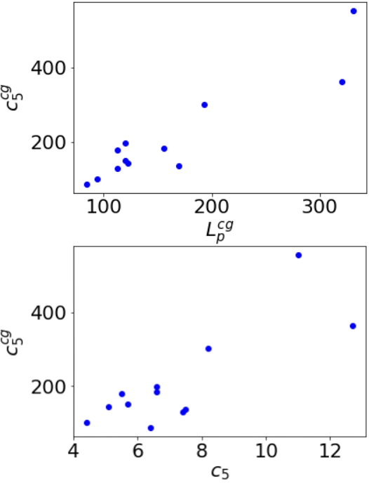
Figure 10: The same as Fig. 5, but inter-community connectivity is defined by taking the average of node weights rather than the sum. Errors are small than symbol sizes. $r^{2}=0.854$ and $r^{2}=0.662$

Fig. 10 presents the Wilson-Cowan results for simplified networks that are a product of a slightly different coarse-graining procedure; the weights of the links between two communities is defined as the average (rather than the sum) of the weights of the links connecting the nodes constituting the two communities. This results in a worsening of the correlations, which suggests that using the sum of weights is the more conducive method to our goal of producing coarse-grained networks that are adequately representative of the original ones.

VI.2.2 Intermediate coarse-graining

Finally, we conducted the same analysis for coarse-grained networks of intermediate sizes, computed using the same algorithm but terminated before the maximum of modularity is attained. The results are clearly unchanged in this third scale, as may be observed in Fig. 10, which is perhaps unsurprising, but it serves as a sanity check.

References

- Sporns (2003) O. Sporns, Complexity 8, 56–60 (2003).
- Zalesky et al. (2010) A. Zalesky, A. Fornito, and E. T. Bullmore, NeuroImage 53, 1197–1207 (2010).
- Bassett and Sporns (2017) D. S. Bassett and O. Sporns, Nature Neuroscience 20, 353 (2017).
- Bullmore and Sporns (2009) E. Bullmore and O. Sporns, Nat Rev Neurosci 10, 186–198 (2009).
- Rosen and Halgren (2021) B. Q. Rosen and E. Halgren, bioRxiv (2021), 10.1101/2021.06.07.447453.
- Jbabdi et al. (2015) S. Jbabdi, S. N. Sotiropoulos, S. N. Haber, D. C. Van Essen, and T. Behrens, Nat Neurosci 18, 1546 (2015).
- Shi and Toga (2017) Y. Shi and A. W. Toga, Molecular Psychiatry 22, 1230 (2017).
- Hagmann et al. (2010) P. Hagmann, O. Sporns, N. Madan, L. Cammoun, R. Pienaar, W. V. J., R. Meuli, J.-P. Thiran, and P. E. Grant, Proc Natl Acad Sci U S A 107, 19067–19072 (2010).
- Raichle (2009) M. E. Raichle, Journal of Neuroscience 29, 12729 (2009).
- Lang et al. (2012) E. W. Lang, A. M. Tomé, I. R. Keck, J. M. Górriz-Sáez, and C. G. Puntonet, Computational Intelligence and Neuroscience 2012, 1–21 (2012).
- Eguíluz et al. (2005) V. M. Eguíluz, D. R. Chialvo, G. A. Cecchi, M. Baliki, and A. V. Apkarian, Phys. Rev. Lett. 94, 018102 (2005).
- Heuvel et al. (2008) M. Heuvel, C. Stam, M. Boersma, and H. Hulshoff Pol, NeuroImage 43, 528 (2008).
- Oizumi et al. (2014) M. Oizumi, L. Albantakis, and G. Tononi, PLoS Comput Biol 10 (2014).
- Baars (2005) B. J. Baars, Progress in Brain Research The Boundaries of Consciousness: Neurobiology and Neuropathology , 45–53 (2005).
- Adams and Petruccione (2020) B. Adams and F. Petruccione, AVS Quantum Sci. 2, 022901 (2020).
- Smith et al. (2021) J. Smith, H. Zadeh Haghighi, D. Salahub, and C. Simon, Sci Rep 11, 6287 (2021).
- Zadeh-Haghighi and Simon (2021) H. Zadeh-Haghighi and C. Simon, Sci Rep 11, 12121 (2021).
- Hameroff and Penrose (2014) S. Hameroff and R. Penrose, Phys. Life Rev. 11, 39 (2014).
- Fisher (2014) M. Fisher, Ann. Phys. 61, 593 (2014).
- Girvan and Newman (2002) M. Girvan and M. E. J. Newman, Proceedings of the National Academy of Sciences 99, 7821 (2002).
- Capocci et al. (2005) A. Capocci, V. Servedio, G. Caldarelli, and F. Colaiori, Physica A: Statistical Mechanics and its Applications 352, 669 (2005).
- Blondel et al. (2008) V. D. Blondel, J.-L. Guillaume, R. Lambiotte, and E. Lefebvre, J. Stat. Mech. 2008, P10008 (2008).
- Wilson and Cowan (1972) H. R. Wilson and J. D. Cowan, Biophys J. 12, 1 (1972).
- Muldoon et al. (2016) S. F. Muldoon, F. Pasqualetti, S. Gu, M. Cieslak, S. T. Grafton, J. M. Vettel, and D. S. Bassett, PLOS Computational Biology 12, 1 (2016).
- Bansal et al. (2018a) K. Bansal, J. D. Medaglia, D. S. Bassett, J. M. Vettel, and S. F. Muldoon, PLOS Computational Biology 14, 1 (2018a).
- Kora et al. (2023) Y. Kora, S. Salhi, J. Davidsen, and C. Simon, Phys. Rev. E 107, 054308 (2023).
- Fraiman et al. (2009) D. Fraiman, P. Balenzuela, J. Foss, and D. R. Chialvo, Phys. Rev. E 79, 061922 (2009).
- Marinazzo et al. (2014) D. Marinazzo, M. Pellicoro, G.-R. Wu, L. Angelini, J. M. Cortes, and S. Stramaglia, PLoS ONE 9 (2014).
- Bak et al. (1988) P. Bak, C. Tang, and K. Wiesenfeld, Phys. Rev. A 38, 364 (1988).
- Massobrio et al. (2015) P. Massobrio, V. Pasquale, and S. Martinoia, Scientific Reports 5, 10578 (2015).
- Korchinski et al. (2021) D. J. Korchinski, J. G. Orlandi, S.-W. Son, and J. Davidsen, Phys. Rev. X 11, 021059 (2021).
- Abeyasinghe et al. (2018) P. M. Abeyasinghe, D. R. de Paula, H. Khajehabdollahi, S. R. Valluri, A. M. Owen, and A. Soddu, Brain connectivity 8 (2018).
- Abeyasinghe et al. (2020) P. M. Abeyasinghe, M. Aiello, E. Nichols, C. Cavaliere, S. Fiorenza, O. Masotta, P. Borrelli, A. M. Owen, A. Estraneo, and A. Soddu, J. Clin. Med. 9, 1342 (2020).
- Waxman and Bennett (1972) S. G. Waxman and M. V. Bennett, Nat New Biol 238 (1972).
- Bansal et al. (2018b) K. Bansal, J. Nakuci, and S. F. Muldoon, Current Opinion in Neurobiology 52, 42 (2018b), systems Neuroscience.
- (36) For a more detailed analysis of this model, see Ref. Kora et al., 2023.
- Metropolis et al. (1953) N. Metropolis, N. Rosenbluth, A. W. Rosenbluth, A. H. Teller, and E. Teller, J. Chem. Phys. 21, 1087 (1953).
- Stam and Reijneveld (2007) C. J. Stam and J. C. Reijneveld, Nonlinear Biomed Phys. 1:3 (2007), 10.1186/1753-4631-1-3.
- (39) While global efficiency and characteristic path length are equivalent (and opposing) ways to measure the well-connectedness of a graph, we chose to employ the former for the bulk of our calculations for computational efficiency reasons. However, where it concerns the Wilson-Cowan model, we chose to compute the characteristic path length for a sample of networks in order to simplify the process of comparing with previous work that utilized the characteristic path length to measure well-connectedness.
- Salhi et al. (2023) S. Salhi, Y. Kora, G. Ham, H. Z. Haghighi, and C. Simon, PLoS ONE 18, e0272688 (2023).