Alpha-Fair Routing in Urban Air Mobility with Risk-Aware Constraints

Abstract

In the vision of urban air mobility, air transport systems serve the demands of urban communities by routing flight traffic in networks formed by vertiports and flight corridors. We develop a routing algorithm to ensure that the air traffic flow fairly serves the demand of multiple communities subject to stochastic network capacity constraints. This algorithm guarantees that the flight traffic volume allocated to different communities satisfies the alpha-fairness conditions, a commonly used family of fairness conditions in resource allocation. It further ensures robust satisfaction of stochastic network capacity constraints by bounding the coherent risk measures of capacity violation. We prove that implementing the proposed algorithm is equivalent to solving a convex optimization problem. We demonstrate the proposed algorithm using a case study based on the city of Austin. Compared with one that maximizes the total served demands, the proposed algorithm promotes even distributions of served demands for different communities.

I Introduction

Urban air mobility (UAM) aims to provide sustainable and accessible air transport services at low altitudes in metropolitan areas [1, 2]. Recent advancements in electrification, automation, and digitalization have enabled many technological innovations for aviation, such as those for electric vertical take-off and landing aircraft, unmanned aerial systems, and automated air traffic management. Together these innovations will facilitate a wide range of urban aviation tasks, such as passenger mobility, goods delivery, and emergency services.

One challenge in UAM is to allocate limited and uncertain amounts of network resources fairly to different flights. On the one hand, the capacity of the transportation network in UAM, defined by its vertiports and flight corridors, is both limited—due to construction budget [3], noise pollution regulations [4], and safety concerns for navigation [5]—and uncertain—due to stochastic weather conditions, dynamic obstacles [6], and emergencies. The air traffic routed through the network must robustly satisfy these uncertain capacity constraints. On the other hand, the network must support flights between multiple origins and destinations to serve the demands of different user groups.

The existing methods for air traffic management with fairness considerations mainly focus on allocating delays fairly among different flights. These methods allocate delays to different flights by minimizing certain deviations from a target allocation [7, 8, 9]. This target allocation typically satisfies certain desired principles, such as the ration-by-distance principle, which prioritizes flights according to their flight distances [8, 9], or the ration-by-schedule principle, which preserves the first-scheduled-first-served ordering of flights [10]. Different planning methods minimize different deviation functions, such as the amount of overtaking and number of reversals in the ordering of flights [11, 12], the amount by which the total delay exceeds the maximum expected delay along a route [10, 12], the proportion of the total delays allocated to an airline divided by its peak requests [13, 14], and the lexicographical worst-case deviation among different flights [15]. Recent results in UAM also consider fairness under uncertainties [16].

However, these existing methods focus on fairness among the service providers, such as different airlines, rather than fairness among service receivers, such as users from different communities. In particular, they seek fair distribution of flight delays based on the flight distances [8, 9] or the schedules requested by different airlines [10], not the origin and destination of the flights. In the context of UAM, a paramount question regarding how to ensure fairness in serving the demands of multiple user communities—which is among the largest barriers to UAM’s community acceptance [1, 2]—is, to our best knowledge, still an open question.

We develop a routing algorithm for UAM to fairly serve the demands of different communities subject to stochastic network capacity. This algorithm has two key features. First, it ensures that the air traffic volume serving the demands of different communities satisfies the alpha fairness conditions, a general class of fairness conditions in resource allocation that includes many different fairness notions, such as proportional fairness, total delay fairness, and max-min fairness [17, 18]. Second, it ensures robust satisfaction of stochastic capacities constraints of vertiports and flight corridors by bounding the coherent risk measures of capacity violation. We prove that implementing this algorithm is equivalent to solving a convex optimization problem with conic constraints. We demonstrate this algorithm using a case study based on the city of Austin. Compared with one that maximizes the total demands served, the proposed algorithm consistently promotes even distributions of demands served for different communities.

II Alpha-fair routing in urban air mobility

We introduce the alpha-fair routing problem in urban air mobility (UAM). The idea is to maximize the total utility function of the services in the form of payloads allocated to different communities subject to network flow constraints.

Throughout, we use the following notations. We let $\mathbb{R}$, $\mathbb{R}_{\geq 0}$, and $\mathbb{N}$ denote the set of real numbers, nonnegative real numbers, and nonnegative integers, respectively. We let $0_{n}$ and $1_{n}$ denote the $n$-dimensional zero vector and all 1’s vector, respectively. Given $n_{1},n_{2}\in\mathbb{N}$, we let $[n_{1},n_{2}]$ denote the set of integers between $n_{1}$ and $n_{2}$. We let $\Delta_{n}\subset\mathbb{R}^{n}$ denote the $n$-dimensional probability simplex.

II-A Nodes, links, and routes

We model the transportation network using a directed graph $\mathcal{G}$ composed of a set of nodes $\mathcal{N}=\{1,2,\ldots,n_{n}\}$, each of which corresponds to either a vertiport or a waypoint that marks the intersection of multiple flight corridors, and a set of links $\mathcal{L}=\{1,2,\ldots,n_{l}\}$, each of which corresponds to a flight corridor. Each link is an ordered pair of distinct nodes, where the first and second nodes are the “tail” and “head” of the link, respectively. A route is a sequence of links connected in a head-to-tail fashion. We let $\mathcal{R}=\{1,2,\ldots,n_{r}\}$ denote a set of routes, which does not necessarily contain all possible routes in $\mathcal{G}$. We will also use the notion of community. Each route serves the demands of one or several of the total of $n_{c}\in\mathbb{N}$ communities.

II-B Incidence matrices

We encode the topology of a graph $\mathcal{G}$ using the notion of incidence matrices, which, depending on its definition, describes which nodes each link connects, which links each route contains, and which communities’ demands each route serves. In particular, we describe the incidence relationship between nodes and links using the node-link incidence matrix $E\in\mathbb{R}^{n_{n}\times n_{l}}$. The entry $E_{ij}$ in matrix $E$ is associated with node $i$ and link $j$ as follows:

$$E_{ij}=\begin{cases}1,&\text{if node $i$ is the head of link $j$,}\\ -1,&\text{if node $i$ is the tail of link $j$,}\\ 0,&\text{otherwise.}\end{cases}$$ (1)

Similarly, we describe the incidence relationship between links and routes using the link-route incidence matrix $F\in\mathbb{R}^{n_{l}\times n_{r}}$. The entry $F_{ij}$ in matrix $F$ is associated with link $i$ and route $j$ as follows:

$$F_{ij}=\begin{cases}1,&\text{if route $j$ contains link $i$,}\\ 0,&\text{otherwise.}\end{cases}$$ (2)

Finally, we describe the incidence relationship between communities and routes using the community-route incidence matrix $H\in\mathbb{R}^{n_{c}\times n_{r}}$. The entry $H_{ij}$ in matrix $H$ is associated with community $i$ and route $j$ as follows:

$$H_{ij}=\begin{cases}1,&\text{if route $j$ serves the demand of community $i$,}\\ 0,&\text{otherwise.}\end{cases}$$ (3)

II-C Balanced flow constraints

To ensure that the number of vehicles at each node is balanced, the total number of incoming vehicles must match the number of outgoing vehicles at each node. We denote the number of aircraft vehicles on different links per unit time using the vehicle flow vector $y\in\mathbb{R}^{n_{l}}$. In particular, the entry $[y]_{k}$ in vector $y$ denotes the number of vehicles that use link $k$. We formulate this constraint as follows:

$$Ey=0_{n_{n}},\,y\geq 0_{n_{l}}.$$ (4)

If the constraint in (4) is violated, the vehicles will start to accumulate at some nodes, which cause unwanted crowding.

II-D Vehicle capacity constraints

Whenever multiple routes share an overlapping link, the amount of payload transported on each route is jointly constrained by the number of vehicles scheduled on the overlapping link. To model this constraint, we first define the payload flow vector $z\in\mathbb{R}^{n_{r}}$ such that $z_{i}$ denotes the number of payloads transported along route $i$. Next, based on the link-route incidence matrix in (2), the vehicle flow vector and the payload flow vector jointly satisfy the following constraint:

$$Fz\leq y,\,z\geq 0_{n_{r}}.$$ (5)

II-E Node and link capacity constraints

To ensure collision-free operation, the number of vehicles on each link and node must be bounded. To model these constraints, we let $c\in\mathbb{R}_{\geq 0}^{n_{n}}$ and $d\in\mathbb{R}_{\geq 0}^{n_{l}}$ denote the nominal node and link flow volume, respectively. In particular, the values of $c_{i}$ and $d_{j}$ denote the maximum number of vehicles that enter node $i$ and link $j$, respectively. Furthermore, we define a weighting matrix $K\in\mathbb{R}^{n_{n}\times n_{l}}$ such that $K=\max\{E,0\}$ i.e., each element in $K$ is the elementawise maximum of the corresponding element in matrix $E$ and zero. Based on these matrices, we define the following node and link capacity constraints:

$$Ky\leq(1+\epsilon)c,\,y\leq(1+\epsilon)d,$$ (6)

where $\epsilon\in\mathbb{R}_{\geq 0}$ is a tolerance parameter. The constraints in (6) state that the number of vehicles on each node or link does not exceed the corresponding nominal value by more than $100\epsilon$ percent.

II-F Alpha-fair routing problem

Given the network constraints, we aim to route the air traffic to serve the demands of multiple communities. Throughout we assume each community has sufficiently high demands and we aim to maximize the demands we serve for each community without violating network capacity constraints. To this end, we introduce the alpha-fair routing approach, which determines the amount of payload allocated to each community via optimization. Let $x\in\mathbb{R}^{n_{c}}_{\geq 0}$ denote the community demand vector such that $x_{k}$ denotes the payload demand we allocate to community $k$. The idea of alpha-fair routing is to find an optimal allocation $x^{\star}\in\mathbb{R}^{n_{c}}$ by solving the following optimization problem:

$$\begin{array}[]{ll}\underset{x,y,z}{\mbox{maximize}}&\sum_{k=1}^{n_{c}}\psi_{k}(x_{k})\\ \mbox{subject to}&Ey=0_{n_{n}},\,x=Hz,\,Fz\leq y,\\ &Ky\leq(1+\epsilon)c,\,y\leq(1+\epsilon)d,\\ &y\geq 0_{n_{l}},\,z\geq 0_{n_{r}}\\ \end{array}$$ (7)

where $\alpha\in[0,\infty)$ is a fairness parameter, and $\psi_{\alpha}$ is the $\alpha$-utility function defined as follows

$$\psi_{k}(x_{k})=\begin{cases}\log(x_{k}),&\text{if $\alpha=1$},\\ \frac{x_{k}^{1-\alpha}}{1-\alpha},&\text{if $\alpha\geq 0,\alpha\neq 1$}.\end{cases}$$ (8)

The goal of optimization (7) is to find an optimal payload allocation that satisfies a set of fairness condition. In particular, let $x^{\star}\in\mathbb{R}^{n_{c}}$ be optimal for optimization (7). Then one can prove that, for any $x\in\mathbb{R}^{n_{c}}$ such that $(x,y,z)$ satisfies the constraints in (7) for some $y\in\mathbb{R}^{n_{l}}$ and $z\in\mathbb{R}^{n_{r}}$, we must have

$$\sum_{k=1}^{n_{c}}\frac{x_{k}-x_{k}^{\star}}{(x^{\star}_{k})^{\alpha}}\leq 0.$$ (9)

The conditions in (9) are known as the $\alpha$-fairness conditions [17]. They include many popular notions of fairness in the network resource allocation literature, including proportional fairness, total delay fairness, and max-min fairness. We refer the interested readers to [17, Sec. 2.4] and the references therein for further details on alpha-fairness.

III Risk-aware alpha-fair routing

One drawback of the routing problem in (7) is that it ignores the effects of uncertainty in air mobility. In the following, we introduce a variation of the routing problem in (7) that accounts for uncertain network capacity, which occurs due to, for instance, weather conditions and emergency shutdowns. To this end, we denote the capacity parameter as $\omega\coloneqq\begin{bmatrix}c^{\top}&d^{\top}\end{bmatrix}^{\top}$. Furthermore, we make the following assumption on $\omega$.

Assumption 1.

The parameter vector $\omega\coloneqq\begin{bmatrix}c^{\top}&d^{\top}\end{bmatrix}^{\top}$ is a discrete random variable with $N\in\mathbb{N}$ possible outcomes. Its sample space is given by $\{\omega^{i}\coloneqq\begin{bmatrix}(c^{i})^{\top}&(d^{i})^{\top}\end{bmatrix}^{\top}\}_{i=1}^{N}$, where $c^{i}\in\mathbb{R}_{\geq 0}^{n_{n}}$ and $d^{i}\in\mathbb{R}_{\geq 0}^{n_{l}}$ for all $i\in[1,N]$.

In the following, we will discuss how to modify the capacity constraints in (6) and the corresponding routing problem in (7) under Assumption (1)

III-A Alpha-fair routing with risk-aware constraints

If $(c,d)=(c^{i},d^{i})$ for some $i\in[1,d]$, then the capacity constraints in (6) is equivalent to a constraint on the optimal value of a linear program. In this case, one can show that (6) is equivalent to

$$h_{i}^{\star}\leq\epsilon,$$ (10)

where $h_{i}^{\star}\in\mathbb{R}$ is the optimal value of the following linear program

$$\begin{array}[]{ll}\underset{h_{i}}{\mbox{minimize}}&h_{i}\\ \mbox{subject to}&Ky\leq(1+h_{i})c^{i},\,y\leq(1+h_{i})d^{i},\,h_{i}\geq 0.\end{array}$$ (11)

To see the equivalence between (6) and (10), notice that (6) implies that $h_{i}=\epsilon$ satisfies the constraints in (11), hence (10) must hold. On the other hand, if (10) holds, then letting $h_{i}=h_{i}^{\star}$ in the constraints in (11) implies that (6).

To constrain the capacity violation under Assumption 1, we define a scalar-valued random variable $\eta$ with a finite sample space $\{h^{\star}_{1},h^{\star}_{2},\ldots,h_{N}^{\star}\}$, where $h^{\star}_{i}$ is the optimal value of the deterministic linear program in (11). In addition, we introduce a family of functions, denoted by $\rho_{\delta}:\mathbb{R}^{n_{l}}\to\mathbb{R}$ for some parameter $\delta\in(0,1)$, such that

$$\rho_{\delta}(y)=\max_{q\in\mathbb{Q(\delta)}}\,q^{\top}h^{\star},$$ (12)

where set $\mathbb{Q}(\delta)\subset\Delta_{N}$ is a closed and convex set that satisfies the following assumption.

Assumption 2.

There exists $p\in\Delta_{N}$ and a closed, convex, and proper function $g_{\delta}:\mathbb{R}^{N}\to\mathbb{R}\cup\{\infty\}$ such that $g_{\delta}(p)<0$ and $\mathbb{Q}(\delta)\coloneqq\left\{q\in\mathbb{R}^{N}|g_{\delta}(q)\leq 0\right\}\cap\Delta_{N}$. Furthermore, $g_{\delta_{1}}(q)>g_{\delta_{2}}(q)$ for all $q\in\Delta_{N}$ and $0<\delta_{1}<\delta_{2}<1$.

Function $g_{\delta}$ provides a coherent risk measure of random variable $\eta$. In particular, the representation theorem states that a coherent risk measure of a random variable $\eta$—which is characterized by the monotonicity, translational invariance, positive homogeneity, subadditivity properties [19]—is equivalent to the maximum expectation of this variable over a convex and closed set of probability distributions [19, Prop. 4.1]. Hence, under Assumption 2, (12) implies that $g_{\delta}(y)$ is is a coherent risk measure of $\eta$, where $\delta\in[0,1]$ is an uncertainty parameter: the volume of set $\mathbb{Q}(\delta)$ increases as $\delta$ increases. Many common risk measures satisfy Assumption 2. See Appendix for some examples.

Based on function (12), we propose to replace the stochastic constraint in (6) with the following:

$$\rho_{\delta}(y)\leq\epsilon.$$ (13)

Under Assumption 1, if $\mathbb{Q}(\delta)=\{p\}$, then (13) implies that the constraints in (6) only hold in expectation. On the other hand, if $\mathbb{Q}(\delta)=\Delta_{N}$, then (10) holds for all $i\in[1,d]$. By ranging $\delta$ within the interval $[0,1]$, the constraint in (13) ensures different tradeoffs between a risk-neutral and a risk-averse variation of the stochastic constraints in (6).

By replacing the constraints in (6) with its risk-aware variation in (12), we obtain a risk-aware variation of the routing problem in (7), given as follows:

$$\begin{array}[]{ll}\underset{x,y,z}{\mbox{maximize}}&\sum_{k=1}^{n_{c}}\psi_{k}(x_{k})\\ \mbox{subject to}&Ey=0_{n_{n}},\,x=Hz,\,Fz\leq y,\\ &\rho_{\delta}(y)\leq\epsilon,\,y\geq 0_{n_{l}},\,z\geq 0_{n_{r}}.\end{array}$$ (14)

III-B Simplification of risk-aware constraints

Optimization (14) seems challenging to solve: it contains an outer layer optimization over the network flow variables and an inner layer optimization that comes from the definition of the coherent risk measure in (12). In the following, we show that this nested two-layer optimization is equivalent to a single-level convex optimization using duality theory. To this end, we make the following assumption on set $\mathbb{Q}$ in (12).

Assumption 2 states that set $\mathbb{Q}$ is the intersection of the sublevel set of a convex function and the probability simplex. Many popular risk measures—such as the conditional value-at-risk, entropic value-at-risk, and total variation distance—satisfy this assumption. See the Appendix for the detailed formula of some popular risk measures.

Based on Assumption 2, the value of the coherent risk measure in (12) is the optimal value of not only the maximization problem in (12), but also its dual problem, as shown by the following proposition.

Proposition 1.

Suppose that Assumption 1 and Assumption 2 hold. Given $\delta\in(0,1)$ and $y\in\mathbb{R}^{n_{l}}_{\geq 0}$, the value of $\rho_{\delta}(y)$ equals the optimal value of the following optimization problem

$$\begin{array}[]{ll}\underset{w,\lambda,\nu,h}{\mbox{minimize}}&\lambda g_{\delta}^{*}(\frac{1}{\lambda}w)-\nu\\ \mbox{subject to}&Ky\leq(1+h_{i})c^{i},\,y\leq(1+h_{i})d^{i},\,h\geq 0_{N},\\ &w-\nu 1_{N}\geq h,\,\lambda\geq 0,\,i\in[1,N],\end{array}$$ (15)

where $g_{\delta}^{*}:\mathbb{R}^{N}\to\mathbb{R}\cup\{\infty\}$ is the convex conjugate function of $g_{\delta}$, i.e., $g_{\delta}^{*}(w)\coloneqq\sup_{q}\,q^{\top}w-g_{\delta}(w)$ for all $w\in\mathbb{R}^{N}$. Furthermore, we define $0\cdot g_{\delta}^{*}(\frac{1}{0}w)\coloneqq\infty$ for all $w\in\mathbb{R}^{N}$.

Proof.

We first show that the dual problem of the optimization in (12) is as follows:

$$\begin{array}[]{ll}\underset{\lambda,\nu,w}{\mbox{minmize}}&\lambda g_{\delta}^{*}(\frac{1}{\lambda}w)-\nu\\ \mbox{subject to}&w-\nu 1_{N}\geq h^{\star},\,\lambda\geq 0.\end{array}$$ (16)

Notice that we implicitly assume that $\lambda>0$ in (16). The Lagrangian of optimiztaion (16) is given by $L(w,\lambda,\nu,q,\sigma)=\textstyle\lambda g_{\delta}^{*}(\frac{1}{\lambda}w)+q^{\top}(h^{\star}+\nu 1_{N}-w)-\sigma\lambda-\nu.$. The dual problem of optimization (16) is as follows:

$$\begin{array}[]{ll}\underset{q,\sigma}{\mbox{maxmize}}&\underset{w,\lambda,\nu}{\mbox{min}}\,L(w,\lambda,\nu,q,\sigma)\\ \mbox{subject to}&q\geq 0_{N},\,\sigma\geq 0.\end{array}$$ (17)

For any $\lambda>0$, we can show that

$$\textstyle\underset{w}{\mbox{min}}\,\lambda g_{\delta}^{*}(\frac{1}{\lambda}w)-q^{\top}w=\textstyle-\underset{u}{\mbox{max}}\,\lambda q^{\top}u-\lambda g_{\delta}^{*}(u)=-\lambda g_{\delta}(q),$$ (18)

where the last step is due to the fact that $(g_{\delta}^{*})^{*}=g_{\delta}$ when $g_{\delta}$ under Assumption 2 [20, Thm.12.2]. By using (18) we can show the following:

$$\underset{\lambda,\nu,w}{\mbox{min}}\,L(w,\lambda,\nu,q,\sigma)$$ (19)

$$=\underset{\lambda,\nu}{\mbox{min}}\,-\lambda g_{\delta}(q)+q^{\top}(h^{\star}+\nu 1_{N})-\sigma\lambda-\nu$$

$$=\begin{cases}q^{\top}h^{\star},&\text{if }g_{\delta}(q)=-\sigma,\,q^{\top}1_{N}=1,\\ -\infty,&\text{otherwise.}\end{cases}$$

Substituting (19) into (17) gives

$$\begin{array}[]{ll}\underset{q}{\mbox{maxmize}}&\textstyle q^{\top}h^{\star}\\ \mbox{subject to}&q^{\top}1_{N}=1,\,q\geq 0,\,g(q)\leq 0.\end{array}$$ (20)

Notice that, under Assumption 2, optimization (20) is exactly the optimization in (12). Since Assumption 1 and Assumption 2 together imply that optimization (20) is strictly feasible if $q=p$, we conclude that optimization (16) and optimization (20) have the same optimal value.

Finally, suppose that $(w,\lambda,\nu)$ satisfies the constraints in optimization (16). Since $h^{\star}$ satisfies the constraints in (11) for all $i\in[1,N]$, $(w,\lambda,\nu,h^{\star})$ satisfies the constraints in optimization (15). Next, suppose that $(w,\lambda,\nu,h)$ is optimal for optimization (15). Since $h_{i}^{\star}$ is the optimal value of optimization (11) for all $i\in[1,N]$, we necessarily have

$$w-\nu 1_{N}\geq h\geq h^{\star}.$$

Hence $(w,\lambda,\nu)$ satisfies the constraints of optimization (16). Therefore there exists $h\in\mathbb{R}^{n}$ such that $(w,\lambda,\nu,h)$ satisfies the constraints in optimization (16) if and only if $(w,\lambda,\nu)$ satisfies the constraints in optimization (15). Since optimization (15) and optimization (16) have the same objective function, we conclude that the optimal values of the two optimization problems are the same. ∎

Proposition 1 shows that any upper bound on the coherent risk measure in (12) is an upper bound on the optimal value of a convex minimization problem. Based on this observation, the following proposition shows that one can merge said minimization together with the outer-layer maximization in (14) by introducing additional variables and constraints.

Proposition 2.

Suppose that Assumption 1 holds. Optimization (14) is equivalent to the following optimization problem

$$\begin{array}[]{ll}\underset{x,y,z,w,\lambda,\nu,h}{\mbox{maximize}}&\sum_{k=1}^{n_{c}}\psi_{k}(x_{k})\\ \mbox{subject to}&Ey=0_{n_{n}},\,x=Hz,\,Fz\leq y,\\ &Ky\leq(1+h_{i})c^{i},\,y\leq(1+h_{i})d^{i},\\ &w-\nu 1_{N}\geq h,\,y\geq 0_{n_{l}},\,z\geq 0_{n_{r}},\,\,h\geq 0_{N},\\ &\lambda g_{\delta}^{*}(\frac{1}{\lambda}w)-\nu\leq\epsilon,\,\lambda\geq 0,\,i\in[1,N].\end{array}$$ (21)

Proof.

If $(x,y,z,w,\nu,\lambda,h)$ satisfies the constraints in (21), then $(w,\lambda,\nu,h)$ satisfies the constraints in (15). Furthermore, Proposition (1) implies that

$$\textstyle\epsilon\geq\lambda g_{\delta}^{*}(\frac{1}{\lambda}w)-\nu\geq\rho_{\delta}[\zeta_{\mathbb{D}}(y)].$$ (22)

Hence $(x,y,z)$ satisfies the constraints in (14). On the other hand, if $(x,y,z)$ satisfies the constraints in (14), then Proposition 1 implies that there exists $(w,\lambda,\nu,h)$ such that

$$\textstyle\lambda g_{\delta}^{*}(\frac{1}{\lambda}w)-\nu=\rho_{\delta}[\zeta_{\mathbb{D}}(y)]\leq\epsilon.$$ (23)

In other words, $(x,y,z,w,\lambda,\nu,h)$ satisfies the constraints in (21). Therefore, $(x,y,z)$ satisfies the constraints in (14) if and only if there exists $w,\lambda,\nu,h$ such that $(x,y,z,w,\lambda,\nu,h)$ satisfies the constraints in (21). Since optimization (14) and (21) have the same objective function, we complete the proof. ∎

Proposition 2 shows that the risk-aware routing problem in (14) is equivalent to the constrained convex optimization problem in (21). For come common risk measures, the constraints in (21) are either linear or exponential cone constraints. See Appendix for details.

IV Numerical Experiments

We demonstrate the proposed routing algorithm using a case study based on a UAM network in the city of Austin, illuatrated by Fig. 1a. This network serves the demands of $n_{c}=46$ communities, each corresponding to a zip code area in the city of Austin. It contains $n_{n}=17$ nodes, each corresponding to a vertiport; $n_{l}=72$ links, each corresponding to a flight corridor; and $n_{r}=200$ candidate routes, each containing at most five connected flight corridors. We choose the locations of the nodes to be city centers or subcenters that are geographically and societally reconfigurable into vertiports. To simplify air traffic management in UAM, we deploy the links such that there are no intersections between different links. We select the 200 routes based on the public transportation plans and the function of different communities. We choose the capacities of the vertiports and flight corridors based on utilization forecast and safety and noise considerations. We also consider a uniform capacity reduction of $20\%$ and $40\%$ for all vertiports and flight corridors, which occurs with probability $0.3$ and $0.2$, respectively.

We aim to route the network flow of vehicles in the Austin network to fairly serve the demands of all 46 communities subject to constraints on the coherent risk measures of the stochastic link and node capacity violation. We illustrate the routing results obtained by solving optimization (21) using the Frank-Wolfe method [21] (terminated after 100 iterations) in Fig. 1 and Fig. 2. We compare them with the results of maximizing the total community demand served, which is obtained by solving optimization (21) with $\psi_{k}(x_{k})=x_{k}$ for all $k\in[1,n_{c}]$. These results show that optimizing the alpha-utility function promotes even distribution of the demands served for different communities.

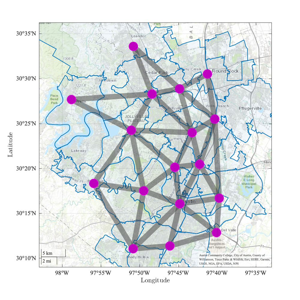
(a) Austin network

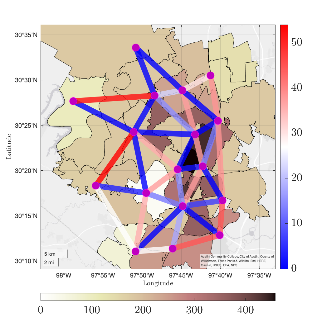
(b) Maximizing the total demand served

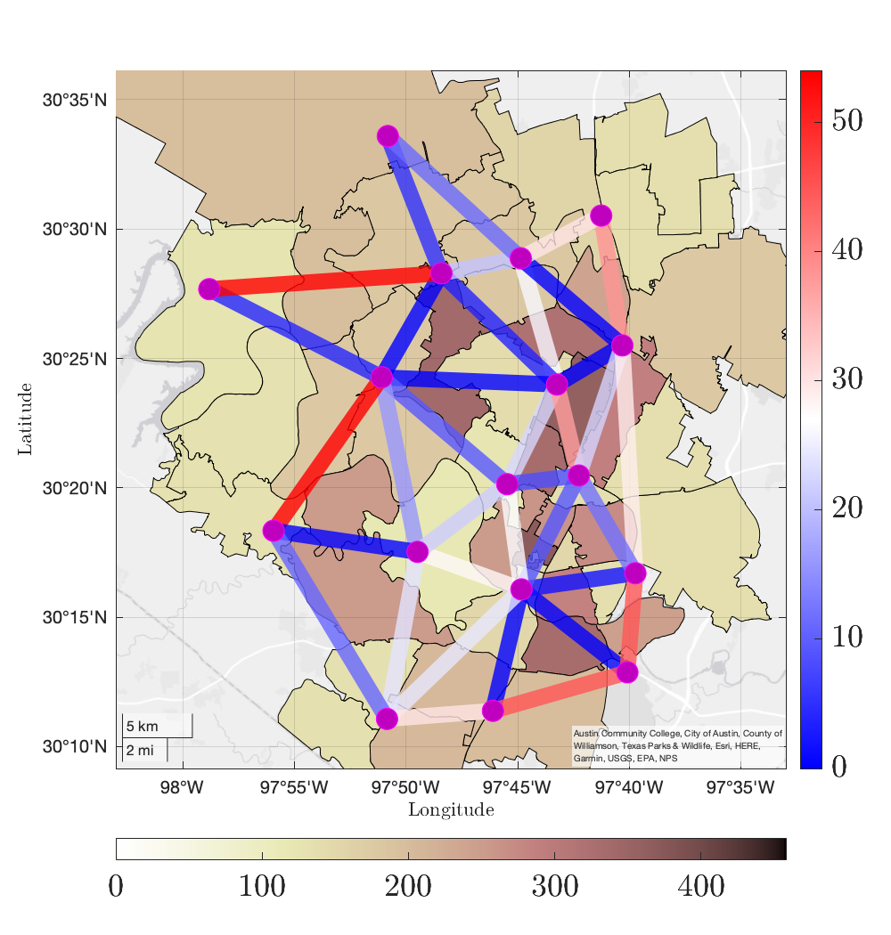
(c) Ensuring alpha-fairness

Figure 1: The Austin network (left), and the average number of flights per hour for different links and communities when maximizing the total community demand served (middle) and ensuring alpha-fairness (right) subject to capacity constraints based on the conditional value-at-risk.

(a) Conditional value-at-risk

(b) Total-variation distance

Figure 2: The average number of flights per hour assigned to different communities subject to capacity constraints based on different risk measures and different values of parameter $\delta$. The red and blue markers show the results when maximizing the total demand served and ensuring alpha-fairness, respectively.

V Conclusion

We develop a routing algorithm to fairly serve the demands of multiple communities in UAM subject to risk-aware constraints. We ensure the fairness of the demands served for different communities by maximizing the sum of alpha-utility functions, and the robust satisfaction of stochastic link and node capacity constraints via bounding the coherent risk measures of capacity violation. We demonstrate our results using a UAM network based on the city of Austin.

However, our current results still have several limitations. For example, the proposed algorithm does not consider dynamic changes in link and node capacity to time-dependent noise regulations. For future work, we plan to extend our results to dynamic routing as well as simultaneous network design and traffic routing in UAM.

Appendix: Function Common risk measures

We provide some common examples of formulas of the function $g_{\delta}$ in Assumption 2 for some common coherent risk measures, along with its convex conjugate function, which appears in optimization (21).

V-A Conditional value-at-risk

For conditional value-at-risk, the function $g$ in Assumption 2 takes the following form:

$$g_{\delta}(q)\coloneqq\left\lVert\mathop{\rm diag}(p)^{-1}q\right\rVert_{\infty}-1/(1-\delta)$$ (24)

We can show, for any $r\in\mathbb{R}^{N}$, that

$$g_{\delta}^{*}(r) =1/(1-\delta)+\sup_{q}\,r^{\top}q-\left\lVert\mathop{\rm diag}(p)^{-1}q\right\rVert_{\infty}$$ (25)

$$=1/(1-\delta)+\sup_{u}\,r^{\top}\mathop{\rm diag}(p)u-\left\lVert u\right\rVert_{\infty}$$

$$=\begin{cases}1/(1-\delta),&\text{if }\left\lVert\mathop{\rm diag}(p)r\right\rVert_{1}\leq 1,\\ \infty,&\text{otherwise.}\end{cases}$$

V-B Entropic value-at-risk

For entropic value-at-risk, the function $g$ in Assumption 2 takes the following form:

$$g_{\delta}(q)\coloneqq\begin{cases}\sum_{i=1}^{N}q_{i}\ln(q_{i}/p_{i})+\ln(1-\delta),&\text{if }q\in\Delta_{N},\\ \infty,&\text{otherwise.}\end{cases}$$ (26)

Given $r\in\mathbb{R}^{N}$, we have

$$\textstyle g_{\delta}^{*}(r)=-\ln(1-\delta)+\sup_{q\in\Delta_{N}}\,r^{\top}q-\sum_{i=1}^{N}q_{i}\ln(q_{i}/p_{i})$$ (27)

Using the KKT conditions, we can show that the supreme in (27) is attained if there exists $\beta\in\mathbb{R}$ such that $0=r_{i}-\ln(q_{i}/p_{i})-\beta-1$ for all $i\in[N]$ and $1=q^{\top}1_{N},$. Substituting these conditions into (27) shows that

$$g_{\delta}^{*}(r)=-\ln(1-\delta)+\ln(p^{\top}\exp(r))$$ (28)

where $\exp(r)$ is the elementwise exponential of $r$. In this case, one can show that $g_{\delta}^{*}(r)$ is the optimal value of an exponential cone program. See [22, Sec. 4.1.2] for a related discussion.

V-C Total variation distance

For the total variance distance [23], the function $g$ in Assumption 2 takes the following form:

$$g_{\delta}(q)\coloneqq\left\lVert q-p\right\rVert_{1}-2\delta.$$ (29)

Given $r\in\mathbb{R}^{N}$, we can show that

$$g_{\delta}^{*}(r) =2\delta+r^{\top}p+\sup_{q}\,r^{\top}(q-p)-\left\lVert q-p\right\rVert_{1}$$ (30)

$$=\begin{cases}2\delta+r^{\top}p,&\text{if }\left\lVert r\right\rVert_{\infty}\leq 1,\\ \infty,&\text{otherwise.}\end{cases}$$

References

- [1] A. P. Cohen, S. A. Shaheen, and E. M. Farrar, “Urban air mobility: History, ecosystem, market potential, and challenges,” IEEE Trans. Intell. Transp. Syst., vol. 22, no. 9, pp. 6074–6087, 2021.
- [2] T. Biehle, “Social sustainable urban air mobility in Europe,” Sustainability, vol. 14, no. 15, p. 9312, 2022.
- [3] Y. Yu, M. Wang, M. Mesbahi, and U. Topcu, “Vertiport selection in hybrid air-ground transportation networks via mathematical programs with equilibrium constraints,” IEEE Trans. Control Netw. Syst., pp. 1–12, 2023.
- [4] Z. Gao, A. Porcayo, and J.-P. Clarke, “Developing virtual acoustic terrain for urban air mobility trajectory planning,” Transp. Res. D: Transport Environ., vol. 120, p. 103794, 2023.
- [5] Q. Wei, Z. Gao, J.-P. Clarke, and U. Topcu, “Risk-aware urban air mobility network design with overflow redundancy,” arXiv preprint arXiv:2306.05581, 2023.
- [6] P. Wu, J. Xie, Y. Liu, and J. Chen, “Risk-bounded and fairness-aware path planning for urban air mobility operations under uncertainty,” Aerosp. Sci. Technol., vol. 127, p. 107738, 2022.
- [7] M. Pelegrín, C. d’Ambrosio, R. Delmas, and Y. Hamadi, “Urban air mobility: From complex tactical conflict resolution to network design and fairness insights,” Optim. Methods Software, pp. 1–33, 2023.
- [8] T. Vossen, M. Ball, R. Hoffman, and M. Wambsganss, “A general approach to equity in traffic flow management and its application to mitigating exemption bias in ground delay programs,” Air Traffic Control Quart., vol. 11, no. 4, pp. 277–292, 2003.
- [9] M. O. Ball, R. Hoffman, and A. Mukherjee, “Ground delay program planning under uncertainty based on the ration-by-distance principle,” Transp. Sci., vol. 44, no. 1, pp. 1–14, 2010.
- [10] C. Barnhart, D. Bertsimas, C. Caramanis, and D. Fearing, “Equitable and efficient coordination in traffic flow management,” Transp. Sci., vol. 46, no. 2, pp. 262–280, 2012.
- [11] D. Bertsimas and S. Gupta, “Fairness and collaboration in network air traffic flow management: an optimization approach,” Transp. Sci., vol. 50, no. 1, pp. 57–76, 2016.
- [12] C. Chin, K. Gopalakrishnan, M. Egorov, A. Evans, and H. Balakrishnan, “Efficiency and fairness in unmanned air traffic flow management,” IEEE Transactions on Intelligent Transportation Systems, vol. 22, no. 9, pp. 5939–5951, 2021.
- [13] J. Fairbrother, K. G. Zografos, and K. D. Glazebrook, “A slot-scheduling mechanism at congested airports that incorporates efficiency, fairness, and airline preferences,” Transp. Sci, vol. 54, no. 1, pp. 115–138, 2020.
- [14] K. G. Zografos and Y. Jiang, “A bi-objective efficiency-fairness model for scheduling slots at congested airports,” Transp. Res. C: Emerging Technol., vol. 102, pp. 336–350, 2019.
- [15] A. Jacquillat and V. Vaze, “Interairline equity in airport scheduling interventions,” Transp. Sci., vol. 52, no. 4, pp. 941–964, 2018.
- [16] L. Sun, P. Wei, and W. Xie, “Fair and risk-averse urban air mobility resource allocation under uncertainties,” Available at SSRN 4343979, 2023.
- [17] S. Shakkottai, R. Srikant, et al., “Network optimization and control,” Found. Trends® in Netw., vol. 2, no. 3, pp. 271–379, 2008.
- [18] V. Xinying Chen and J. Hooker, “A guide to formulating fairness in an optimization model,” Ann. Oper. Res., pp. 1–39, 2023.
- [19] P. Artzner, F. Delbaen, J.-M. Eber, and D. Heath, “Coherent measures of risk,” Math. Finance, vol. 9, no. 3, pp. 203–228, 1999.
- [20] R. T. Rockafellar, Convex analysis. Princeton University Press, 2015.
- [21] M. Jaggi, “Revisiting frank-wolfe: Projection-free sparse convex optimization,” in Proc. Int. Conf. Mach. Learn. PMLR, 2013, pp. 427–435.
- [22] A. Dixit, M. Ahmadi, and J. W. Burdick, “Risk-averse receding horizon motion planning,” arXiv preprint arXiv:2204.09596 [eess.SY], 2022.
- [23] ——, “Distributionally robust model predictive control with total variation distance,” IEEE Control Syst. Lett., vol. 6, pp. 3325–3330, 2022.