Prior Mismatch and Adaptation in PnP-ADMM with a Nonconvex Convergence Analysis

Abstract

Plug-and-Play (PnP) priors is a widely-used family of methods for solving imaging inverse problems by integrating physical measurement models with image priors specified using image denoisers. PnP methods have been shown to achieve state-of-the-art performance when the prior is obtained using powerful deep denoisers. Despite extensive work on PnP, the topic of distribution mismatch between the training and testing data has often been overlooked in the PnP literature. This paper presents a set of new theoretical and numerical results on the topic of prior distribution mismatch and domain adaptation for alternating direction method of multipliers (ADMM) variant of PnP. Our theoretical result provides an explicit error bound for PnP-ADMM due to the mismatch between the desired denoiser and the one used for inference. Our analysis contributes to the work in the area by considering the mismatch under nonconvex data-fidelity terms and expansive denoisers. Our first set of numerical results quantifies the impact of the prior distribution mismatch on the performance of PnP-ADMM on the problem of image super-resolution. Our second set of numerical results considers a simple and effective domain adaption strategy that closes the performance gap due to the use of mismatched denoisers. Our results suggest the relative robustness of PnP-ADMM to prior distribution mismatch, while also showing that the performance gap can be significantly reduced with few training samples from the desired distribution.

1 Introduction

Imaging inverse problems consider the recovery of a clean image from its corrupted observation. Such problems arise across the fields of computational imaging, biomedical imaging, and computer vision. As imaging inverse problems are typically ill-posed, solving them requires the use of image priors. While many approaches have been proposed for implementing image priors, the current literature is primarily focused on methods based on training deep learning (DL) models to map noisy observations to clean images [1, 2, 3].

Plug-and-Play (PnP) Priors [4, 5] has emerged as a class of DL algorithms for solving inverse problems by denoisers as image priors. PnP has been successfully used in many applications such as super-resolution, phase retrieval, microscopy, and medical imaging [6, 7, 8, 9, 10, 11, 12]. The success of PnP has resulted in the development of its multiple variants (e.g., PnP-PGM, PnP-SGD, PnP-ADMM. PnP-HQS), strong interest in its theoretical analysis, as well as investigation of its connection to other methods used in inverse problems, such as score matching and denoising diffusion probabilistic models [13, 14, 15, 16, 17, 18, 19, 20, 21, 22, 23, 24, 25, 26, 27].

Despite extensive literature on PnP, the research in the area has mainly focused on the setting where the distribution of the test or inference data is perfectly matched to that of the data used for training the image denoiser. Little work exists for PnP under mismatched priors, where a distribution shift exists between the training and test data. In this paper, we investigate the problem of mismatched priors in PnP-ADMM. We present a new theoretical analysis of PnP-ADMM that accounts for the use of mismatched priors. Unlike most existing work on PnP-ADMM, our theory is compatible with nonconvex data-fidelity terms and expansive denoisers [28, 29, 30, 31, 32]. Our analysis establishes explicit error bounds on the convergence of PnP-ADMM under a well-defined set of assumptions. We validate our theoretical findings by presenting numerical results on the influence of distribution shifts, where the denoiser trained on one dataset (e.g., BreCaHAD or CelebA) is used to recover an image from another dataset (e.g., MetFaces or RxRx1). We additionally present numerical results on a simple domain adaptation strategy for image denoisers that can effectively address data distribution shifts in PnP methods (see Figure 4 for an illustration). Our work thus enriches the current PnP literature by providing novel theoretical and empirical insights into the problem of data distribution shifts in PnP.

All proofs and some details that have been omitted due to space constraints of the main text are included in the supplementary material.

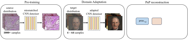
Figure 1: Illustration of domain adaptation in PnP-ADMM. The mismatched denoiser is pre-trained on source distribution (BreCaHAD) and adapted to target distribution (MetFaces) using a few samples. Adapted prior is then plugged into PnP-ADMM algorithm to reconstruct a sample from MetFaces.

2 Background

Inverse problems. Inverse problems involve the recovery of an unknown signal ${\bm{x}}\in\mathbb{R}^{n}$ from a set of noisy measurements ${\bm{y}}={\bm{A}}{\bm{x}}+{\bm{e}}$, where ${\bm{A}}\in\mathbb{R}^{m\times n}$ is the measurement model and ${\bm{e}}$ is the noise. Inverse problems are often formulated and solved as optimization problems of form

$${\widehat{\bm{x}}}\in\mathop{\mathsf{arg\,min}}_{{\bm{x}}\in\mathbb{R}^{n}}f({\bm{x}})\quad\text{with}\quad f({\bm{x}})=g({\bm{x}})+h({\bm{x}})\ ,$$ (1)

where $g$ is the data-fidelity term that measures the consistency with the measurements ${\bm{y}}$ and $h$ is the regularizer that incorporates prior knowledge on ${\bm{x}}$. The least-squares function $g({\bm{x}})=\frac{1}{2}\|{\bm{A}}{\bm{x}}-{\bm{y}}\|_{2}^{2}$ and total variation (TV) function $h({\bm{x}})=\tau\|{\bm{D}}{\bm{x}}\|_{1}$, where ${\bm{D}}$ denotes the image gradient and $\tau>0$ a regularization parameter, are commonly used functions for the data-fidelity term and the regularizer [33, 34].

Deep Learning. DL has gained significant attention in the context of inverse problems [1, 2, 3]. DL methods seek to perform a regularized inversion by learning a mapping from the measurements to the target images parameterized by a deep convolutional neural network (CNN) [35, 36, 37, 38, 39, 40]. Model-based DL (MBDL) refers to a sub-class of DL methods for inverse problems that also integrate the measurement model as part of the deep model [3, 41]. MBDL approaches include methods such as PnP, regularization by denoising (RED), deep unfolding (DU), and deep equilibrium models (DEQ) [42, 43, 44, 45].

Plug-and-Play Priors. PnP is one of the most popular MBDL approaches for solving imaging inverse problems that uses denoisers as priors [4] (see also recent reviews [17, 19]). PnP has been extensively investigated, leading to multiple PnP variants and theoretical analyses [13, 15, 28, 32, 26, 27, 46, 16, 21, 25]. Existing theoretical convergence analyses of PnP differ in the specifics of the assumptions required to ensure the convergence of the corresponding iterations. For example, bounded, averaged, firmly nonexpansive, nonexpansive, residual nonexpansive, or demi-contractive denoisers have been previously considered for designing convergent PnP schemes [13, 30, 14, 32, 25, 22, 28, 47, 20, 23, 48, 49]. The recent work [50] has used an elegant formulation of an MMSE denoiser from [51] to perform a nonconvex convergence analysis of PnP-PGM without any nonexpansiveness assumptions on the denoiser. Another recent line of PnP work has explored specification of the denoiser as a gradient-descent step on a functional parameterized by a deep neural network [26, 52, 25].

PnP-ADMM is summarized in Algorithm 1 [5, 4], where ${\mathsf{D}}_{\sigma}$ is an additive white Gaussian denoiser (AWGN) denoiser, $\gamma>0$ is the penalty parameter, and $\sigma>0$ controls the denoiser strength. PnP-ADMM is based on the alternating direction method of multipliers (ADMM) [53]. Its formulation relies on optimizing in an alternating fashion the augmented Lagrangian associated with the objective function in (1)

$$\phi\left({\bm{x}},{\bm{z}},{\bm{s}}\right)=g({\bm{x}})+h({\bm{z}})+\frac{1}{\gamma}{\bm{s}}^{\mathsf{T}}({\bm{x}}-{\bm{z}})+\frac{1}{2\gamma}\left\|{\bm{x}}-{\bm{z}}\right\|_{2}^{2}.$$ (2)

The theoretical convergence of PnP-ADMM has been explored for convex functions using monotone operator theory [32, 28], for nonconvex regularizer and convex data-fidelity terms [52], and for bounded denoisers [13].

Distribution Shift. Distribution shifts naturally arise in imaging when a DL model trained on one type of data is applied to another. The mismatched DL models due to distribution shifts lead to suboptimal performance. Consequently, there has been interest in mitigating the effect of mismatched DL models [54, 55, 56, 57]. In PnP methods, a mismatch arises when the denoiser is trained on a distribution different from that of the test data. The prior work on denoiser mismatch in PnP is limited [58, 20, 27, 59].

Our contributions. (1) Our first contribution is a new theoretical analysis of PnP-ADMM accounting for the discrepancy between the desired and mismatched denoisers. Such analysis has not been considered in the prior work on PnP-ADMM. Our analysis is broadly applicable in the sense that it does not assume convex data-fidelity terms and nonexpansive denoisers. (2) Our second contribution is a comprehensive numerical study of distribution shifts in PnP through several well-known image datasets on the problem of image super-resolution. (3) Our third contribution is the illustration of simple data adaptation for addressing the problem of distribution shifts in PnP-ADMM. We show that one can successfully close the performance gap in PnP-ADMM due to distribution shifts by adapting the denoiser to the target distribution using very few samples.

3 Proposed Work

This section presents the convergence analysis of PnP-ADMM that accounts for the use of mismatched denoisers. It is worth noting that the theoretical analysis of PnP-ADMM has been previously discussed in [31, 16, 32, 28]. The novelty of our work can be summarized in two aspects: (1) we analyze convergence with the mismatched priors; (2) our theory accommodates nonconvex $g$ and expansive denoisers.

3.1 PnP-ADMM with Mismatched Denoiser

Algorithm 1 PnP-ADMM

1:input: ${\bm{z}}^{0},{\bm{s}}^{0}\in\mathbb{R}^{n}$, parameters $\sigma,\gamma>0$.

2:for $k=1,2,3,\cdots$ do

3:     ${\bm{x}}^{k}\leftarrow{\mathsf{prox}}_{\gamma g}({\bm{z}}^{k-1}-{\bm{s}}^{k-1})$

4:     ${\bm{z}}^{k}\leftarrow{\mathsf{D}}_{\sigma}\left({\bm{x}}^{k}+{\bm{s}}^{k-1}\right)$

5:     ${\bm{s}}^{k}\leftarrow{\bm{s}}^{k-1}+{\bm{x}}^{k}-{\bm{z}}^{k}$

6:end for

We denote the target distribution as $p_{\bm{x}}$ and the mismatched distribution as $\widehat{p}_{\bm{x}}$. The mismatched denoiser ${\mathsf{\widehat{D}}}_{\sigma}$ is a minimum mean squared error (MMSE) estimator for the AWGN denoising problem

$${\bm{v}}={\bm{x}}+{\bm{e}}\quad\text{with}\quad{\bm{x}}\sim\widehat{p}_{\bm{x}},\quad{\bm{e}}\sim{\mathcal{N}}(0,\sigma^{2}{\bm{I}}).$$ (3)

The MMSE denoiser is the conditional mean estimator for (3) and can be expressed as

$${\mathsf{\widehat{D}}}_{\sigma}({\bm{v}})\,\coloneqq\,\mathbb{E}[{\bm{x}}|{\bm{v}}]=\int_{\mathbb{R}^{n}}{\bm{x}}\widehat{p}_{{\bm{x}}|{\bm{v}}}({\bm{x}}|{\bm{v}}){\mathsf{\,d}}{\bm{x}},$$ (4)

where $\widehat{p}_{{\bm{x}}|{\bm{v}}}({\bm{x}}|{\bm{v}})\propto G_{\sigma}({\bm{v}}-{\bm{x}})\widehat{p}_{\bm{x}}({\bm{x}})$, with $G_{\sigma}$ denoting the Gaussian density. We refer to the MMSE estimator ${\mathsf{\widehat{D}}}_{\sigma}$, corresponding to the mismatched data distribution $\widehat{p}_{\bm{x}}$, as the mismatched prior.

Since the integral (4) is generally intractable, in practice, the denoiser corresponds to a deep model trained to minimize the mean squared error (MSE) loss

$${\mathcal{L}}({\mathsf{\widehat{D}}}_{\sigma})=\mathbb{E}\left[\|{\bm{x}}-{\mathsf{\widehat{D}}}_{\sigma}({\bm{v}})\|_{2}^{2}\right].$$ (5)

MMSE denoisers trained using the MSE loss are optimal with respect to the widely used image-quality metrics in denoising, such as signal-to-noise ratio (SNR), and have been extensively used in the PnP literature [50, 27, 60, 24, 61].

When using a mismatched prior in PnP-ADMM, we replace Step 4 in Algorithm 1 by

$${\bm{z}}^{k}\leftarrow{\mathsf{\widehat{D}}}_{\sigma}\left({\bm{x}}^{k}+{\bm{s}}^{k-1}\right),$$ (6)

where ${\mathsf{\widehat{D}}}_{\sigma}$ is the mismatched MMSE denoiser. To avoid confusion, we denote by ${\bm{z}}^{k}$ and ${\overline{\bm{z}}}^{k}$ the outputs of the mismatched and target denoisers at the $k$ iteration, respectively. Consequently, we have ${\overline{\bm{z}}}^{k}={\mathsf{D}}_{\sigma}({\bm{x}}^{k}+{\bm{s}}^{k-1}),$ where ${\mathsf{D}}_{\sigma}$ is the target MMSE denoiser.

3.2 Theoretical Analysis

Our analysis relies on the following set of assumptions that serve as sufficient conditions.

Assumption 1.

The prior distributions $p_{{\bm{x}}}$ and $\widehat{p}_{{\bm{x}}}$, denoted as target and mismatched priors respectively, are non-degenerate over $\mathbb{R}^{n}$.

A distribution is considered degenerate over $\mathbb{R}^{n}$ if its support is confined to a lower-dimensional manifold than the dimensionality of $n$. Assumption 1 is useful to establish an explicit link between a MMSE denoiser and its associated regularizer. For example, the regularizer $h$ associated with the target MMSE denoiser ${\mathsf{D}}_{\sigma}$ can be expressed as (see [51, 50] for background)

$$h({\bm{x}})\,\coloneqq\,\begin{cases}-\frac{1}{2\gamma}\|{\bm{x}}-{\mathsf{D}}_{\sigma}^{-1}({\bm{x}})\|_{2}^{2}+\frac{\sigma^{2}}{\gamma}h_{\sigma}({\mathsf{D}}_{\sigma}^{-1}({\bm{x}}))&\text{for }{\bm{x}}\in{\mathsf{Im}}({\mathsf{D}}_{\sigma})\\ +\infty&\text{for }{\bm{x}}\notin{\mathsf{Im}}({\mathsf{D}}_{\sigma}),\end{cases}$$ (7)

where $\gamma>0$ denotes the penalty parameter, ${\mathsf{D}}_{\sigma}^{-1}:{\mathsf{Im}}({\mathsf{D}}_{\sigma})\rightarrow\mathbb{R}^{n}$ represent a well defined and smooth inverse mapping over ${\mathsf{Im}}({\mathsf{D}}_{\sigma})$, and $h_{\sigma}(\cdot)\,\coloneqq\,-\log(p_{{\bm{u}}}(\cdot))$, with $p_{{\bm{u}}}$ denoting the probability distribution over the AWGN corrupted observations

$${\bm{u}}={\bm{x}}+{\bm{e}}\quad\text{with}\quad{\bm{x}}\sim p_{\bm{x}},\quad{\bm{e}}\sim{\mathcal{N}}(0,\sigma^{2}{\bm{I}}),$$

(the derivation is provided in Section E.1 for completeness). Note that the smoothness of both ${\mathsf{D}}_{\sigma}^{-1}$ and $h_{\sigma}$ guarantees the smoothness of the function $h$. Additionally, similar connection exist between the mismatched MMSE denoiser ${\mathsf{\widehat{D}}}_{\sigma}$ and the regularizer ${\hat{h}}({\bm{x}})$, with ${\hat{h}}_{\sigma}(\cdot)\,\coloneqq\,-\log(\widehat{p}_{{\bm{v}}}(\cdot))$ characterizing the relationship between mismatched denoiser and shifted distribution.

Assumption 2.

The function $g$ is continuously differentiable.

This assumption is a standard assumption used in nonconvex optimization, specifically in the context of inverse problems [62, 63, 64].

Assumption 3.

The data-fidelity term and the implicit regularizers are bounded from below.

Assumption 3 implies that there exists $f^{\ast}>-\infty$ such that $f({\bm{x}})\geq f^{\ast}$ for all ${\bm{x}}\in\mathbb{R}^{n}$.

Assumption 4.

The denoisers ${\mathsf{D}}_{\sigma}$ and ${\mathsf{\widehat{D}}}_{\sigma}$ have the same range ${\mathsf{Im}}({\mathsf{D}}_{\sigma})$. Additionally, functions $h$ and ${\hat{h}}$ associated with ${\mathsf{D}}_{\sigma}$ and ${\mathsf{\widehat{D}}}_{\sigma}$, are continuously differentiable with $L$-Lipschitz continuous gradients over ${\mathsf{Im}}({\mathsf{D}}_{\sigma}).$

It is known (see [51, 50]) that functions $h$ and ${\hat{h}}$ are infinitely differentiable over their ranges. The assumption that the two image denoisers have the same range is also a relatively mild assumption. Ideally, both denoisers would have the same range corresponding to the set of desired images. Assumption 4 is thus a mild extension that further requires Lipschitz continuity of the gradient over the range of denoisers.

Assumption 5.

The mismatched denoiser ${\mathsf{\widehat{D}}}_{\sigma}$ satisfies

$$\|{\mathsf{\widehat{D}}}_{\sigma}({\bm{v}}^{k})-{\mathsf{D}}_{\sigma}({\bm{v}}^{k})\|_{2}\leq\delta_{k},\quad k=1,2,3,\ldots$$

where ${\mathsf{\widehat{D}}}_{\sigma}$ is given in (4) and ${\bm{v}}^{k}={\bm{x}}^{k}+{\bm{s}}^{k-1}$ in Algorithm 1.

Our analysis assumes that at every iteration, PnP-ADMM uses a mismatched MMSE denoiser, derived from a shifted distribution. We consider the case where at iteration $k$ of PnP-ADMM, the distance of the outputs of ${\mathsf{D}}_{\sigma}$ and ${\mathsf{\widehat{D}}}_{\sigma}$ is bounded by a constant $\delta_{k}$.

Assumption 6.

For the sequence $\{{\bm{x}}^{k},{\bm{z}}^{k},{\bm{s}}^{k}\}$ generated by iterations of PnP-ADMM with mismatched MMSE denoiser in Algorithm 1, there exists a constant $R$ such that

$$\left\|{\bm{z}}^{k}-{\bm{z}}^{*}\right\|_{2}\leq R,\quad k=1,2,3,\ldots$$

where $\left({\bm{x}}^{\ast},{\bm{z}}^{\ast},{\bm{s}}^{\ast}\right)$ are stationary points of augmented Lagrangian in (2).

This assumption is a reasonable assumption since many images have bounded pixel values, for example $[0,255]$ or $[0,1]$.

We are now ready to present our convergence result under mismatched MMSE denoisers.

Theorem 1.

Run PnP-ADMM using a mismatched MMSE denoiser for $t\geq 1$ iterations under Assumptions 1-6 with the penalty parameter $0<\gamma\leq 1/(4L)$. Then, we have

$$\mathop{\mathsf{min}}_{1\leq k\leq t}\left\|\nabla f\left({\bm{x}}^{k}\right)\right\|_{2}^{2}\leq\frac{1}{t}\sum_{k=1}^{t}\left\|\nabla f\left({\bm{x}}^{k}\right)\right\|^{2}_{2}\leq\frac{A_{1}}{t}\left(\phi\left({\bm{x}}^{0},{\bm{z}}^{0},{\bm{s}}^{0}\right)-\phi^{\ast}\right)+A_{2}{\overline{\varepsilon}}_{t}$$

where $A_{1}>0$ and $A_{2}>0$ are iteration independent constants, $\phi^{*}=\phi({\bm{x}}^{*},{\bm{z}}^{*},{\bm{s}}^{*})$, and ${\overline{\varepsilon}}_{t}\,\coloneqq\,(1/t)\left(\varepsilon_{1}+\cdots+\varepsilon_{t}\right)$ is the error term that is an average of the quantities $\varepsilon_{k}\,\coloneqq\,{\mathsf{max}}\{\delta_{k},\delta_{k}^{2}\}$. In addition, if the sequence $\{\delta_{i}\}_{i\geq 1}$ is summable, we have that $\|\nabla f({\bm{x}}^{t})\|_{2}\to 0$ as $t\to\infty$.

When we replace the mismatched MMSE denoiser with the target MMSE denoiser, we recover the traditional PnP-ADMM. To highlight the impact of the mismatch, we next provide the same statement but using the target denoiser.

Theorem 2.

Run PnP-ADMM with the MMSE denoiser for $t\geq 1$ iterations under Assumptions 1-4 with the penalty parameter $0<\gamma\leq 1/(4L)$. Then, we have

$$\mathop{\mathsf{min}}_{1\leq k\leq t}\left\|\nabla f\left({\bm{x}}^{k}\right)\right\|_{2}^{2}\leq\frac{1}{t}\sum_{k=1}^{t}\left\|\nabla f({\bm{x}}^{k})\right\|^{2}_{2}\leq\frac{C}{t}\left(\phi({\bm{x}}^{0},{\bm{z}}^{0},{\bm{s}}^{0})-\phi^{\ast}\right),$$

where $C>0$ is a constant independent of iteration.

The proof of Theorem 1 is provided in the appendix. For completeness, we also provide the proof of Theorem 2. Theorem 1 provides insight into the convergence of PnP-ADMM using mismatched MMSE denoisers. It states that if $\delta_{k}$ are summable, the iterates of PnP-ADMM with mismatched denoisers satisfy $\nabla f({\bm{x}}^{t})\to\bm{0}$ as $t\to 0$ and PnP-ADMM converges to a stationary point of the objective function $f$ associated with the target denoiser. On the other hand, if the sequence $\delta_{k}$ is not summable, the convergence is only up to an error term that depends on the distance between the target and mismatched denoisers. Theorem 1 can be viewed as a more flexible alternative for the convergence analyses in [28, 31, 32]. While the analyses in the prior works assume convex $g$ and nonexpansive residual, nonexpansive or bounded denoisers, our analysis considers that denoiser ${\mathsf{D}}_{\sigma}$ is a mismatched MMSE estimator, where the mismatched denoiser distance to the target denoiser is bounded by $\delta_{k}$ at each iteration of PnP-ADMM.

Figure 2: Sample images from the datasets used for training the denoisers. From left to right: MetFaces [65], CelebA [66], AFHQ [67], RxRx1 [68], and  BreCaHAD [69].

In conclusion, PnP-ADMM using a mismatched MMSE denoiser approximates the solution obtained by PnP-ADMM using the target MMSE denoiser with an error that depends on the discrepancy between the denoisers. Therefore, one can control the accuracy of PnP-ADMM using mismatched denoisers by controlling the error term ${\overline{\varepsilon}}_{t}$. This error term can be controlled by using domain adaptation techniques for decreasing the distance between mismatched and target denoisers, thus closing the gap in the performances of PnP-ADMM. We numerically validate this observation in Section 4 by considering the fine-tuning of mismatched denoisers to the target distribution with a limited number of samples.

4 Numerical Validation

We consider PnP-ADMM with mismatched and adapted denoisers for the task of image super-resolution. Our first set of results shows how distribution shifts relate to the prior disparities and their impact on PnP recovery performance. Our second set of results shows the impact of domain adaptation on the denoiser gap and PnP performance. We use the traditional $l_{2}$-norm as the data-fidelity term. To provide an objective evaluation of the final image quality, we use two established quantitative metrics: Peak Signal-to-Noise Ratio (PSNR) and Structural Similarity Index (SSIM).

We use DRUNet architecture [12] for all image denoisers. To model prior mismatch, we train denoisers on five image datasets: MetFaces [65], AFHQ [67], CelebA [66], BreCaHAD [69], and RxRx1 [68]. Figure 2 illustrates samples from the datasets. Our training dataset consists of 1000 randomly chosen, resized, or cropped image slices, each measuring $256\times 256$ pixels. Unlike several existing PnP methods [28, 23] that suggest the inclusion of the spectral normalization layers into the CNN to enforce Lipschitz continuity on the denoisers, we directly train denoisers without any nonexpansiveness constraints.

4.1 Impact of Prior Mismatch

The observation model for single image super-resolution is ${\bm{y}}={\bm{S}}{\bm{H}}{\bm{x}}+{\bm{e}}$, where ${\bm{S}}\in\mathbb{R}^{m\times n}$ is a standard $s$-fold downsampling matrix with $n=m\times s^{2}$, ${\bm{H}}\in\mathbb{R}^{n\times n}$ is a convolution with anti-aliasing kernel, and ${\bm{e}}$ is the noise. To compute the proximal map efficiently for the $l_{2}$-norm data-fidelity term (Step 3 in Algorithm 1), we use the closed-form solution outlined in [12, 70]. Similarly to [12], we use four isotropic kernels with different standard deviation $\{0.7,1.2,1.6,2\}$, as well as four anisotropic kernels depicted in Table 1. We perform downsampling at scales of $s=2$ and $s=4$.

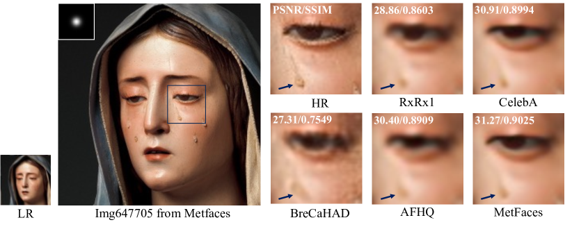
Figure 3: Visual evaluation of PnP-ADMM on image super-resolution using denoisers trained on several datasets. Performance is reported in terms of PSNR (dB) and SSIM for an image from the MetFaces dataset. Images are downsampled by a scale of $s=4$ and convolved with the blur kernel shown on the top left corner of the ground truth image. Note how the disparities in the training distributions of denoisers directly influence the performance of PnP. The denoisers containing images most similar to MetFaces offer the best performance.

Table 1: PSNR (dB) and SSIM values for image super-resolution using PnP-ADMM under different priors on a test set from the MetFaces [65]. We highlighted the best performing and the worst performing priors. BreCaHAD is the worst prior that is also the one visually most different from MetFaces.

Kernels	Prior	$s=2$			$s=4$			Avg
		PSNR	SSIM		PSNR	SSIM		PSNR	SSIM
	BreCaHAD	$\mathbf{31.96}$	$\mathbf{0.8108}$		$\mathbf{28.41}$	$\mathbf{0.6937}$		$\mathbf{30.18}$	$\mathbf{0.7522}$
	RxRx1	$33.45$	$0.8683$		$30.45$	$0.7906$		$31.95$	$0.8294$
	AFHQ	$33.74$	$0.8697$		$30.38$	$0.7825$		$32.06$	$0.8261$
	CelebA	$33.96$	$0.8731$		$30.62$	$0.7906$		$32.29$	$0.8318$
	MetFaces	$\mathbf{34.07}$	$\mathbf{0.8755}$		$\mathbf{31.15}$	$\mathbf{0.8053}$		$\mathbf{32.61}$	$\mathbf{0.8404}$
	BreCaHAD	$\mathbf{30.25}$	$\mathbf{0.7489}$		$\mathbf{28.99}$	$\mathbf{0.7083}$		$\mathbf{29.62}$	$\mathbf{0.7286}$
	RxRx1	$32.22$	$0.8348$		$30.80$	$0.7948$		$31.51$	$0.8148$
	AFHQ	$32.63$	$0.8410$		$31.06$	$0.8014$		$31.84$	$0.8212$
	CelebA	$32.62$	$0.8404$		$31.30$	$0.8070$		$31.96$	$0.8237$
	MetFaces	$\mathbf{32.85}$	$\mathbf{0.8457}$		$\mathbf{31.44}$	$\mathbf{0.8089}$		$\mathbf{32.14}$	$\mathbf{0.8273}$

Figure 3 illustrates the performance of PnP-ADMM using the target and four mismatched denoisers. Note the suboptimal performance of PnP-ADMM using mismatched denoisers trained on the BreCaHAD, RxRx1, CelebA, and AFHQ datasets relative to PnP-ADMM using the target denoiser trained on the MetFaces dataset. Figure 3 illustrates how distribution shifts can lead to mismatched denoisers, subsequently impacting the performance of PnP-ADMM. It’s worth noting that the denoiser trained on the CelebA dataset [66], which consists of facial images similar to MetFaces, is the best-performing mismatched denoiser. Table 1 provides a quantitative evaluation of the PnP-ADMM performance with the target denoiser consistently outperforming all the other denoisers. Notably, the mismatched denoiser trained on the BreCaHAD dataset [69], containing cell images that are most dissimilar to MetFaces, exhibits the worst performance.

4.2 Domain Adaption

In domain adaptation, the pre-trained mismatched denoisers are updated using a limited number of data from the target distribution. We investigate two adaptation scenarios: in the first, we adapt the denoiser initially pre-trained on the BreCaHAD dataset to the MetFaces dataset, and in the second, we use the denoiser initially pre-trained on CelebA for adaptation to the RxRx1 dataset.

Figure 4 illustrates the influence of domain adaptation on denoising and PnP-ADMM. The reported results are tested on RxRx1 and MetFaces datasets for the super-resolution task. The kernel used is shown on the top left corner of the ground truth image in Figure 3 and the images are downsampled at the scale of $s=4$. Note how the denoising performance improves as we increase the number of images used for domain adaptation. This indicates that domain adaptation reduces the distance of mismatched and target denoisers. Additionally, note the direct correlation between the denoising capabilities of priors and the performance of PnP-ADMM. Figure 4 shows that the performance of PnP-ADMM with mismatched denoisers can be significantly improved by adapting the mismatched denoiser to the target distribution, even with just four images from the target distribution.

Figure 5 presents visual examples illustrating domain adaptation in PnP-ADMM for image super-resolution. The recovery performance is shown for two test images from the MetFaces using adapted denoisers against both target and mismatched denoisers. The experiment was conducted under the same settings as those in Figure 3. Note the effectiveness of domain adaptation in mitigating the impact of distribution shifts on PnP-ADMM. Table 2 provides quantitative results of several adapted priors on the test data. The results presented in Table 2 show the substantial impact of domain adaptation, using a limited number of data, in significantly narrowing the performance gap that emerges as a consequence of distribution shifts.

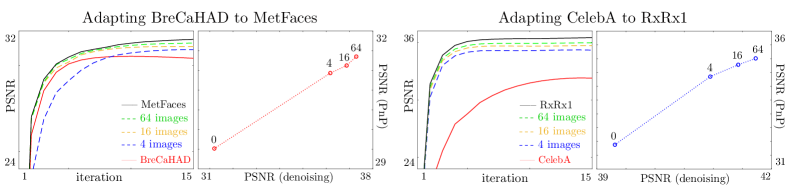
Figure 4: Illustration of prior mismatch and adaption in PnP-ADMM, where a denoiser trained on one dataset (BreCaHAD  [69] or CelebA [66]) is used to recover an image from another dataset (MetFaces [65] or RxRx1 [68]). We plot the convergence of PnP-ADMM in terms of PSNR (first and third figures) and the influence of adapted denoisers on the performance of PnP-ADMM (second and fourth figures). Note how adaptation with even few samples is enough to nearly close the performance gap in PnP-ADMM.

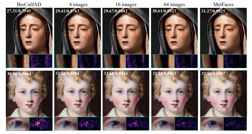
Figure 5: Visual comparison on super-resolution with target (MetFaces), mismatched (BreCaHAD), and adapted priors on two MetFaces test images. The images are downsampled by the scale of $s=4$. The performance is reported in terms of PSNR (dB) and SSIM. Note how the recovery performance increases by adaptation of mismatched priors to a larger set of images from the target distribution.

Table 2: PSNR (dB) and SSIM comparison of super-resolution with mismatched, target, and adapted denoisers for the test set from MetFaces, averaged for indicated kernels. We highlighted the target, mismatched, and the best adapted priors.

Kernels	Prior	$s=2$			$s=4$			Avg
		PSNR	SSIM		PSNR	SSIM		PSNR	SSIM
	BreCaHAD	$\mathbf{31.96}$	$\mathbf{0.8108}$		$\mathbf{28.41}$	$\mathbf{0.6937}$		$\mathbf{30.18}$	$\mathbf{0.7522}$
	4 imgs	$32.51$	$0.8510$		$30.57$	$0.7934$		$31.54$	$0.8222$
	16 imgs	$33.10$	$0.8611$		$30.65$	$0.7961$		$31.89$	$0.8293$
	32 imgs	$33.30$	$0.8649$		$30.81$	$0.8001$		$32.05$	$0.8325$
	64 imgs	$\mathbf{33.59}$	$\mathbf{0.8698}$		$\mathbf{30.84}$	$\mathbf{0.7994}$		$\mathbf{32.21}$	$\mathbf{0.8346}$
	MetFaces	$\mathbf{34.07}$	$\mathbf{0.8755}$		$\mathbf{31.15}$	$\mathbf{0.8053}$		$\mathbf{32.61}$	$\mathbf{0.8404}$
	BreCaHAD	$\mathbf{30.25}$	$\mathbf{0.7489}$		$\mathbf{28.99}$	$\mathbf{0.7083}$		$\mathbf{29.62}$	$\mathbf{0.7286}$
	4 imgs	$31.59$	$0.8215$		$30.86$	$0.7957$		$31.22$	$0.8086$
	16 imgs	$32.19$	$0.8334$		$31.05$	$0.8009$		$31.62$	$0.8171$
	32 imgs	$32.34$	$0.8371$		$31.18$	$0.8044$		$31.76$	$0.8207$
	64 imgs	$\mathbf{32.47}$	$\mathbf{0.8397}$		$\mathbf{31.26}$	$\mathbf{0.8059}$		$\mathbf{31.86}$	$\mathbf{0.8228}$
	MetFaces	$\mathbf{32.85}$	$\mathbf{0.8457}$		$\mathbf{31.44}$	$\mathbf{0.8089}$		$\mathbf{32.14}$	$\mathbf{0.8273}$

5 Conclusion

The work presented in this paper investigates the influence of using mismatched denoisers in PnP-ADMM, presents the corresponding theoretical analysis in terms of convergence, investigates the effect of mismatch on image super-resolution, and shows the ability of domain adaptation to reduce the effect of distribution mismatch. The theoretical results in this paper extend the recent PnP work by accommodating mismatched priors while eliminating the need for convex data-fidelity and nonexpansive denoiser assumptions. The empirical validation of PnP-ADMM involving mismatched priors and the domain adaptation strategy highlights the direct relationship between the gap in priors and the subsequent performance gap in the PnP-ADMM recovery, effectively reflecting the influence of distribution shifts on image priors.

Limitations

The basis of our analysis in this study relies on the assumption that the denoiser used in the inference accurately computes the MMSE denoiser for both target and mismatched distributions. While this assumption aligns well with deep denoisers trained via the MSE loss, it does not directly extend to denoisers trained using alternative loss functions, such as the $l_{1}$-norm or SSIM. As is customary in theoretical research, our analysis remains valid only under the fulfillment of these assumptions, which could potentially restrict its practical applicability. In our future work, we aim to enhance the results presented here by exploring new PnP strategies that can relax these convergence assumptions.

Reproducibility Statement

We have provided the anonymous source code in the supplementary materials. The included README.md file contains detailed instructions on how to run the code and reproduce the results reported in the paper. The algorithm’s pseudo-code is outlined in Algorithm 1, and for more comprehensive information about training, parameter selection, and other details, please refer to the Supplementary Section G. Additionally, for the theoretical findings presented in section 3, complete proofs, along with further clarifications on the assumptions and additional contextual information, can be found in the appendices A-E.

Ethics Statement

To the best of our knowledge, this work does not give rise to any significant ethical concerns.

Supplementary Material

Appendix A Proof of Theorem 1

Theorem.

Run PnP-ADMM with mismatched MMSE denoiser for $t\geq 1$ iterations under Assumptions 1-6 with the penalty parameter $0<\gamma\leq 1/(4L)$. Then, we have

$$\mathop{\mathsf{min}}_{1\leq k\leq t}\left\|\nabla f\left({\bm{x}}^{k}\right)\right\|_{2}^{2}\leq\frac{1}{t}\sum_{k=1}^{t}\left\|\nabla f\left({\bm{x}}^{k}\right)\right\|^{2}_{2}\leq\frac{A_{1}}{t}\left(\phi\left({\bm{x}}^{0},{\bm{z}}^{0},{\bm{s}}^{0}\right)-\phi^{\ast}\right)+A_{2}{\overline{\varepsilon}}_{t}$$

where $A_{1}>0$ and $A_{2}>0$ are iteration independent constants, $\phi^{*}=\phi({\bm{x}}^{*},{\bm{z}}^{*},{\bm{s}}^{*})$, $\varepsilon_{k}\,\coloneqq\,{\mathsf{max}}\{\delta_{k},\delta_{k}^{2}\}$, and ${\overline{\varepsilon}}_{t}\,\coloneqq\,(1/t)\left(\varepsilon_{1}+\cdots+\varepsilon_{t}\right)$. In addition, if the sequence of distances of denoisers $\{\delta_{i}\}_{i\geq 1}$ is summable, we have that $\|\nabla f({\bm{x}}^{t})\|_{2}\to 0$ as $t\to\infty$..

Proof.

Note that from Lemma 1, we have

$$\left\|{\bm{z}}^{k}-{\bm{z}}^{k-1}\right\|_{2}^{2} \leq\frac{2\gamma}{1-2\gamma L-2\gamma^{2}L^{2}}\left(\phi\left({\bm{x}}^{k-1},{\bm{z}}^{k-1},{\bm{s}}^{k-1}\right)-\phi\left({\bm{x}}^{k},{\bm{z}}^{k},{\bm{s}}^{k}\right)\right)$$

$$+\frac{3}{4\left(1-2\gamma L-2\gamma^{2}L^{2}\right)}\ \delta_{k}^{2}+\frac{4R}{1-2\gamma L-2\gamma^{2}L^{2}}\ \delta_{k}.$$ (8)

From the optimality conditions of the target MMSE denoiser ${\mathsf{D}}_{\sigma}$ and proximal operator, for ${\overline{\bm{z}}}^{k}\in{\mathsf{Im}}({\mathsf{D}}_{\sigma})$, we have

$$\nabla h\left({\overline{\bm{z}}}^{k}\right)+\frac{1}{\gamma}\left({\overline{\bm{z}}}^{k}-{\bm{x}}^{k}-{\bm{s}}^{k-1}\right)=\bm{0}\quad\text{and}\quad\nabla g\left({\bm{x}}^{k}\right)+\frac{1}{\gamma}\left({\bm{x}}^{k}+{\bm{s}}^{k-1}-{\bm{z}}^{k-1}\right)=\bm{0}.$$

From this equation, for the objective function defined in (1), we can write

$$\left\|\nabla f\left({\bm{x}}^{k}\right)\right\|_{2} =\left\|\nabla g\left({\bm{x}}^{k}\right)+\nabla h\left({\bm{x}}^{k}\right)\right\|_{2}$$

$$=\left\|\nabla g\left({\bm{x}}^{k}\right)+\frac{1}{\gamma}\left({\bm{x}}^{k}+{\bm{s}}^{k-1}-{\bm{z}}^{k-1}\right)+\nabla h\left({\bm{x}}^{k}\right)+\frac{1}{\gamma}\left({\bm{z}}^{k-1}-{\bm{x}}^{k}-{\bm{s}}^{k-1}\right)\right\|_{2}$$

$$=\left\|\nabla h\left({\overline{\bm{z}}}^{k}\right)+\frac{1}{\gamma}\left({\overline{\bm{z}}}^{k}-{\bm{x}}^{k}-{\bm{s}}^{k-1}\right)+\nabla h\left({\bm{x}}^{k}\right)-\nabla h\left({\overline{\bm{z}}}^{k}\right)+\frac{1}{\gamma}\left({\bm{z}}^{k-1}-{\overline{\bm{z}}}^{k}\right)\right\|_{2}$$

$$=\left\|\nabla h\left({\bm{x}}^{k}\right)-\nabla h\left({\bm{z}}^{k}\right)+\nabla h\left({\bm{z}}^{k}\right)-\nabla h\left({\overline{\bm{z}}}^{k}\right)+\frac{1}{\gamma}\left({\bm{z}}^{k-1}-{\overline{\bm{z}}}^{k}\right)\right\|_{2}$$

$$\leq\left\|\nabla h\left({\bm{x}}^{k}\right)-\nabla h\left({\bm{z}}^{k}\right)\right\|_{2}+\left\|\nabla h\left({\bm{z}}^{k}\right)-\nabla h\left({\overline{\bm{z}}}^{k}\right)\right\|_{2}+\frac{1}{\gamma}\left\|{\bm{z}}^{k-1}-{\overline{\bm{z}}}^{k}\right\|_{2}$$

$$\leq L\left\|{\bm{x}}^{k}-{\bm{z}}^{k}\right\|_{2}+L\left\|{\bm{z}}^{k}-{\overline{\bm{z}}}^{k}\right\|_{2}+\frac{1}{\gamma}\left\|{\bm{z}}^{k-1}-{\bm{z}}^{k}\right\|_{2}+\frac{1}{\gamma}\left\|{\bm{z}}^{k}-{\overline{\bm{z}}}^{k}\right\|_{2}$$

$$\leq\left(\frac{1}{\gamma}+\gamma L^{2}\right)\left\|{\bm{z}}^{k}-{\bm{z}}^{k-1}\right\|_{2}+\left(\frac{1}{\gamma}+L\right)\delta_{k},$$

where we used triangle inequality in the first and second inequality. We also used

$$\left\|{\bm{x}}^{k}-{\bm{z}}^{k}\right\|_{2}\leq\left\|{\bm{s}}^{k}-{\bm{s}}^{k-1}\right\|_{2}=\gamma\left\|\nabla h({\bm{z}}^{k})-\nabla h({\bm{z}}^{k-1})\right\|_{2}\leq\gamma L\left\|{\bm{z}}^{k}-{\bm{z}}^{k-1}\right\|_{2}$$

and Assumption 5 in the last inequality. By squaring both sides and using $(a+b)^{2}\leq 2a^{2}+2b^{2}$, we get

$$\left\|\nabla f\left({\bm{x}}^{k}\right)\right\|^{2}_{2}\leq 2\left(\frac{1}{\gamma}+\gamma L^{2}\right)^{2}\left\|{\bm{z}}^{k}-{\bm{z}}^{k-1}\right\|^{2}_{2}+2\left(\frac{1}{\gamma}+L\right)^{2}\delta_{k}^{2}.$$

By using the result from equation (Theorem), we obtain

$$\left\|\nabla f\left({\bm{x}}^{k}\right)\right\|^{2}_{2} \leq\frac{4\left(1+\gamma^{2}L^{2}\right)^{2}}{\gamma\left(1-2\gamma L-2\gamma^{2}L^{2}\right)}\left(\phi\left({\bm{x}}^{k-1},{\bm{z}}^{k-1},{\bm{s}}^{k-1}\right)-\phi\left({\bm{x}}^{k},{\bm{z}}^{k},{\bm{s}}^{k}\right)\right)$$

$$+\left(\frac{3\left(1+\gamma^{2}L^{2}\right)^{2}}{2\gamma^{2}\left(1-2\gamma L-2\gamma^{2}L^{2}\right)}+\frac{2\left(1+\gamma L\right)^{2}}{\gamma^{2}}\right)\delta_{k}^{2}+\frac{8R\left(1+\gamma^{2}L^{2}\right)^{2}}{\gamma^{2}\left(1-2\gamma L-2\gamma^{2}L^{2}\right)}\delta_{k}.$$ (9)

By averaging both sides of the bound over $t\geq 1$ and using the definition of error in $\varepsilon_{k}\,\coloneqq\,{\mathsf{max}}\{\delta_{k},\delta_{k}^{2}\}$, we get

$$\mathop{\mathsf{min}}_{1\leq k\leq t}\left\|\nabla f\left({\bm{x}}^{k}\right)\right\|_{2}^{2}\leq\frac{1}{t}\sum_{k=1}^{t}\left\|\nabla f\left({\bm{x}}^{k}\right)\right\|^{2}_{2} \leq\frac{A_{1}}{t}\left(\phi\left({\bm{x}}^{0},{\bm{z}}^{0},{\bm{s}}^{0}\right)-\phi\left({\bm{x}}^{t},{\bm{z}}^{t},{\bm{s}}^{t}\right)\right)+A_{2}{\overline{\varepsilon}}_{t}$$

$$\leq\frac{A_{1}}{t}\left(\phi\left({\bm{x}}^{0},{\bm{z}}^{0},{\bm{s}}^{0}\right)-\phi^{\ast}\right)+A_{2}{\overline{\varepsilon}}_{t},$$ (10)

where ${\overline{\varepsilon}}_{t}\,\coloneqq\,(1/t)\left(\varepsilon_{1}+\cdots+\varepsilon_{t}\right)$, $A_{1}\,\coloneqq\,4\left(1+\gamma^{2}L^{2}\right)^{2}/\left(\gamma\left(1-2\gamma L-2\gamma^{2}L^{2}\right)\right)$,

$A_{2}\,\coloneqq\,\left(\left(3+16R\right)\left(1+\gamma^{2}L^{2}\right)/\left(2\gamma^{2}\left(1-2\gamma L-2\gamma^{2}L^{2}\right)\right)+2\left(1/\gamma+L\right)^{2}\right)$, and we used the fact that augmented Lagrangian $\phi$ is bounded from below $\left(\phi^{*}\leq\phi\left({\bm{x}}^{t},{\bm{z}}^{t},{\bm{s}}^{t}\right)\right)$ from Lemma 2 . Note that we used the following inequality to get the result in equation (Theorem)

$$\left(\frac{3\left(1+\gamma^{2}L^{2}\right)^{2}}{2\gamma^{2}\left(1-2\gamma L-2\gamma^{2}L^{2}\right)}+2\left(\frac{1}{\gamma}+L\right)^{2}\right)\delta_{k}^{2}+\frac{8R\left(1+\gamma^{2}L^{2}\right)^{2}}{\gamma^{2}\left(1-2\gamma L-2\gamma^{2}L^{2}\right)}\delta_{k}$$

$$\leq{\mathsf{max}}\{\delta_{k},\delta_{k}^{2}\}\left(\frac{3\left(1+\gamma^{2}L^{2}\right)^{2}}{2\gamma^{2}\left(1-2\gamma L-2\gamma^{2}L^{2}\right)}+2\left(\frac{1}{\gamma}+L\right)^{2}+\frac{8R\left(1+\gamma^{2}L^{2}\right)^{2}}{\gamma^{2}\left(1-2\gamma L-2\gamma^{2}L^{2}\right)}\right)$$

$$=\left(\frac{\left(3+16R\right)\left(1+\gamma^{2}L^{2}\right)^{2}}{2\gamma^{2}\left(1-2\gamma L-2\gamma^{2}L^{2}\right)}+2\left(\frac{1}{\gamma}+L\right)^{2}\right)\varepsilon_{k}.$$

Note that if the sequence of distances of denoisers $\{\delta_{i}\}_{i\geq 1}$ is summable, then $\{\varepsilon_{i}={\mathsf{max}}\{\delta_{i},\delta_{i}^{2}\}\}_{i\geq 1}$ is also be summable. Consequently, $\|\nabla f({\bm{x}}^{t})\|_{2}\to 0$ as $t\to\infty$. ∎

Remark 1. Note that by using (Theorem) when the sequence $\{\delta_{i}\}_{i\geq 1}$ is summable, we have

$$\frac{1}{t}\sum_{k=1}^{t}\left\|{\bm{z}}^{k}-{\bm{z}}^{k-1}\right\|^{2}_{2}\leq 0\quad\text{as}\quad t\to\infty,$$ (11)

which ensures that $\|{\bm{z}}^{k}-{\bm{z}}^{k-1}\|_{2}\to 0$ as $k\to\infty$. Since

$$\left\|{\bm{s}}^{k}-{\bm{s}}^{k-1}\right\|_{2}\leq\gamma L\left\|{\bm{z}}^{k}-{\bm{z}}^{k-1}\right\|_{2}\quad\text{and}\quad\left\|{\bm{s}}^{k}-{\bm{s}}^{k-1}\right\|_{2}=\left\|{\bm{x}}^{k}-{\bm{z}}^{k}\right\|_{2},$$ (12)

we conclude that $\|{\bm{x}}^{k}-{\bm{x}}^{k-1}\|_{2}\to 0$ and $\|{\bm{s}}^{k}-{\bm{s}}^{k-1}\|_{2}\to 0$ as $k\to\infty$.

Appendix B Useful results for Theorem 1

Lemma 1.

Assume that Assumptions 1-6 hold and let the sequence $\{{\bm{x}}^{k},{\bm{z}}^{k},{\bm{s}}^{k}\}$ be generated via iterations of PnP-ADMM with mismatched MMSE denoiser using the penalty parameter $0<\gamma\leq 1/(4L)$. Then for the augmented Lagrangian defined in (2), we have that

$$\phi\left({\bm{x}}^{k},{\bm{z}}^{k},{\bm{s}}^{k}\right)\leq\phi\left({\bm{x}}^{k-1},{\bm{z}}^{k-1},{\bm{s}}^{k-1}\right)-\left(\frac{1-2\gamma L-2\gamma^{2}L^{2}}{2\gamma}\right)\left\|{\bm{z}}^{k}-{\bm{z}}^{k-1}\right\|_{2}^{2}+\frac{3}{8\gamma}\delta_{k}^{2}+\frac{2R}{\gamma}\delta_{k}.$$

where $R$ is defined in Assumption 6.

Proof.

From the smoothness of ${\hat{h}}$ for any ${\bm{z}}^{k}\in{\mathsf{Im}}({\mathsf{D}}_{\sigma})$ in Assumption 4, the optimality condition for the mismatched MMSE denoiser, and the Lagrange multiplier update rule in the form of ${\bm{s}}^{k}={\bm{s}}^{k-1}+{\bm{x}}^{k}-{\bm{z}}^{k}$, we have

$$\nabla{\hat{h}}\left({\bm{z}}^{k}\right)=\frac{1}{\gamma}\left({\bm{s}}^{k-1}+{\bm{x}}^{k}-{\bm{z}}^{k}\right)=\frac{1}{\gamma}{\bm{s}}^{k}$$

and

$$\left\|{\bm{s}}^{k}-{\bm{s}}^{k-1}\right\|_{2}=\left\|\gamma\nabla{\hat{h}}\left({\bm{z}}^{k}\right)-\gamma\nabla{\hat{h}}\left({\bm{z}}^{k-1}\right)\right\|_{2}\leq\gamma L\left\|{\bm{z}}^{k}-{\bm{z}}^{k-1}\right\|_{2},$$ (13)

where we used $L-$Lipschitz continuity of $\nabla{\hat{h}}$ from Assumption (4) in the last inequality. From this equation and the Lagrange multiplier update rule, we have

$$\phi\left({\bm{x}}^{k},{\bm{z}}^{k},{\bm{s}}^{k}\right)-\phi\left({\bm{x}}^{k},{\bm{z}}^{k},{\bm{s}}^{k-1}\right) =\frac{1}{\gamma}\left({\bm{s}}^{k}-{\bm{s}}^{k-1}\right)^{\mathsf{T}}\left({\bm{x}}^{k}-{\bm{z}}^{k}\right)=\frac{1}{\gamma}\left\|{\bm{s}}^{k}-{\bm{s}}^{k-1}\right\|_{2}^{2}$$

$$\leq\gamma L^{2}\left\|{\bm{z}}^{k}-{\bm{z}}^{k-1}\right\|_{2}^{2}.$$ (14)

From the fact that $h$ (regularizer associated with target MMSE denoiser ${\mathsf{D}}_{\sigma}$) has a $L-$Lipschitz continuous gradient over the set ${\mathsf{Im}}({\mathsf{D}}_{\sigma})$ (Assumption 4), we have

$$h\left({\overline{\bm{z}}}^{k}\right)-h\left({\bm{z}}^{k-1}\right)\leq\nabla h\left({\overline{\bm{z}}}^{k}\right)^{\mathsf{T}}\left({\overline{\bm{z}}}^{k}-{\bm{z}}^{k-1}\right)+\frac{L}{2}\left\|{\overline{\bm{z}}}^{k}-{\bm{z}}^{k-1}\right\|_{2}^{2},$$ (15)

where ${\overline{\bm{z}}}^{k}={\mathsf{D}}_{\sigma}({\bm{x}}^{k}+{\bm{s}}^{k-1})$. From the smoothness of $h$ for any ${\overline{\bm{z}}}^{k}\in{\mathsf{Im}}({\mathsf{D}}_{\sigma})$, the optimality condition for mismatched MMSE denoiser, and the Lagrange multiplier update rule ${\bm{s}}^{k}={\bm{s}}^{k-1}+{\bm{x}}^{k}-{\bm{z}}^{k}$, we have

$$\nabla h\left({\overline{\bm{z}}}^{k}\right)=\frac{1}{\gamma}\left({\bm{x}}^{k}+{\bm{s}}^{k-1}-{\overline{\bm{z}}}^{k}\right)=\frac{1}{\gamma}{\bm{s}}^{k}+\frac{1}{\gamma}\left({\bm{z}}^{k}-{\overline{\bm{z}}}^{k}\right).$$ (16)

By combining equations (15) and (16), we obtain

$$h\left({\overline{\bm{z}}}^{k}\right)-h\left({\bm{z}}^{k-1}\right)\leq\frac{1}{\gamma}\left({\bm{s}}^{k}\right)^{\mathsf{T}}\left({\overline{\bm{z}}}^{k}-{\bm{z}}^{k-1}\right)+\frac{1}{\gamma}\left({\bm{z}}^{k}-{\overline{\bm{z}}}^{k}\right)^{\mathsf{T}}\left({\overline{\bm{z}}}^{k}-{\bm{z}}^{k-1}\right)+\frac{L}{2}\left\|{\overline{\bm{z}}}^{k}-{\bm{z}}^{k-1}\right\|_{2}^{2}.$$ (17)

For the target MMSE denoiser ${\mathsf{D}}_{\sigma}$, we know that ${\overline{\bm{z}}}^{k}\in{\mathsf{Im}}({\mathsf{D}}_{\sigma})$ minimizes

$$\psi_{\gamma h}\left({\bm{z}}\right)\,\coloneqq\,\frac{1}{2\gamma}\left\|{\bm{z}}-\left({\bm{x}}^{k}+{\bm{s}}^{k-1}\right)\right\|_{2}^{2}+h\left({\bm{z}}\right).$$ (18)

From Assumption 4, we know that $\nabla h$ is $L-$Lipschitz continuous over ${\mathsf{Im}}({\mathsf{D}}_{\sigma})$, which implies

$$\left\|\nabla\psi_{\gamma h}\left({\bm{u}}\right)-\nabla\psi_{\gamma h}\left({\bm{v}}\right)\right\|_{2}\leq\left(\frac{1}{\gamma}+L\right)\left\|{\bm{u}}-{\bm{v}}\right\|_{2}\quad\forall{\bm{u}},{\bm{v}}\in{\mathsf{Im}}({\mathsf{D}}_{\sigma}).$$

From the smoothness of $\psi_{\gamma h}$ and the fact that ${\overline{\bm{z}}}^{k}$ minimizes it, we have

$$\psi_{\gamma h}\left({\bm{z}}^{k}\right) \leq\psi_{\gamma h}\left({\overline{\bm{z}}}^{k}\right)+\nabla\psi_{\gamma h}\left({\overline{\bm{z}}}^{k}\right)^{\mathsf{T}}\left({\bm{z}}^{k}-{\overline{\bm{z}}}^{k}\right)+\left(\frac{1}{2\gamma}+\frac{L}{2}\right)\left\|{\bm{z}}^{k}-{\overline{\bm{z}}}^{k}\right\|_{2}^{2}$$

$$=\psi_{\gamma h}\left({\overline{\bm{z}}}^{k}\right)+\left(\frac{1}{2\gamma}+\frac{L}{2}\right)\left\|{\bm{z}}^{k}-{\overline{\bm{z}}}^{k}\right\|_{2}^{2}.$$

By using the definition of function $\psi_{\gamma h}$ in (18), the Lagrange multiplier update rule ${\bm{s}}^{k}={\bm{s}}^{k-1}+{\bm{x}}^{k}-{\bm{z}}^{k}$ and rearranging the terms, we obtain

$$h\left({\bm{z}}^{k}\right)-h\left({\overline{\bm{z}}}^{k}\right) \leq\frac{1}{2\gamma}\left\|{\overline{\bm{z}}}^{k}-\left({\bm{x}}^{k}+{\bm{s}}^{k-1}\right)\right\|_{2}^{2}-\frac{1}{2\gamma}\left\|{\bm{z}}^{k}-\left({\bm{x}}^{k}+{\bm{s}}^{k-1}\right)\right\|_{2}^{2}+\left(\frac{1}{2\gamma}+\frac{L}{2}\right)\left\|{\bm{z}}^{k}-{\overline{\bm{z}}}^{k}\right\|_{2}^{2}$$

$$=\frac{1}{2\gamma}\left({\overline{\bm{z}}}^{k}+{\bm{z}}^{k}-2\left({\bm{x}}^{k}+{\bm{s}}^{k-1}\right)\right)^{\mathsf{T}}\left({\overline{\bm{z}}}^{k}-{\bm{z}}^{k}\right)+\left(\frac{1}{2\gamma}+\frac{L}{2}\right)\left\|{\bm{z}}^{k}-{\overline{\bm{z}}}^{k}\right\|_{2}^{2}$$

$$=\frac{1}{\gamma}\left({\bm{s}}^{k}\right)^{\mathsf{T}}\left({\bm{z}}^{k}-{\overline{\bm{z}}}^{k}\right)+\frac{1}{2\gamma}\left\|{\bm{z}}^{k}-{\overline{\bm{z}}}^{k}\right\|_{2}^{2}+\left(\frac{1}{2\gamma}+\frac{L}{2}\right)\left\|{\bm{z}}^{k}-{\overline{\bm{z}}}^{k}\right\|_{2}^{2}$$

$$=\frac{1}{\gamma}\left({\bm{s}}^{k}\right)^{\mathsf{T}}\left({\bm{z}}^{k}-{\overline{\bm{z}}}^{k}\right)+\left(\frac{1}{\gamma}+\frac{L}{2}\right)\left\|{\bm{z}}^{k}-{\overline{\bm{z}}}^{k}\right\|_{2}^{2}.$$ (19)

Now for the augmented Lagrangian, we have

$$\phi\left({\bm{x}}^{k},{\bm{z}}^{k},{\bm{s}}^{k-1}\right)-\phi\left({\bm{x}}^{k},{\bm{z}}^{k-1},{\bm{s}}^{k-1}\right) =h\left({\bm{z}}^{k}\right)-h\left({\bm{z}}^{k-1}\right)+\frac{1}{\gamma}\left({{\bm{s}}^{k-1}}\right)^{\mathsf{T}}\left({\bm{z}}^{k-1}-{\bm{z}}^{k}\right)$$

$$\quad+\frac{1}{2\gamma}\left(2{\bm{x}}^{k}-{\bm{z}}^{k}-{\bm{z}}^{k-1}\right)^{\mathsf{T}}\left({\bm{z}}^{k-1}-{\bm{z}}^{k}\right)$$

$$=h\left({\bm{z}}^{k}\right)-h\left({\bm{z}}^{k-1}\right)+\frac{1}{\gamma}\left({{\bm{s}}^{k-1}}\right)^{\mathsf{T}}\left({\bm{z}}^{k-1}-{\bm{z}}^{k}\right)$$

$$\quad+\frac{1}{\gamma}\left({\bm{s}}^{k}-{\bm{s}}^{k-1}\right)^{\mathsf{T}}\left({\bm{z}}^{k-1}-{\bm{z}}^{k}\right)-\frac{1}{2\gamma}\left\|{\bm{z}}^{k}-{\bm{z}}^{k-1}\right\|^{2}_{2}$$

$$=h\left({\bm{z}}^{k}\right)-h\left({\overline{\bm{z}}}^{k}\right)+h\left({\overline{\bm{z}}}^{k}\right)-h\left({\bm{z}}^{k-1}\right)$$

$$\quad+\frac{1}{\gamma}\left({{\bm{s}}^{k}}\right)^{\mathsf{T}}\left({\bm{z}}^{k-1}-{\bm{z}}^{k}\right)-\frac{1}{2\gamma}\left\|{\bm{z}}^{k}-{\bm{z}}^{k-1}\right\|^{2}_{2},$$ (20)

where we used the Lagrange multiplier update rule in the second equality. By plugging (17) and (B) into (B) and rearranging the terms, we obtain

$$\phi\left({\bm{x}}^{k},{\bm{z}}^{k},{\bm{s}}^{k-1}\right) -\phi\left({\bm{x}}^{k},{\bm{z}}^{k-1},{\bm{s}}^{k-1}\right)\leq\frac{1}{\gamma}\left({\bm{z}}^{k}-{\overline{\bm{z}}}^{k}\right)^{\mathsf{T}}\left({\overline{\bm{z}}}^{k}-{\bm{z}}^{k-1}\right)+\frac{L}{2}\left\|{\overline{\bm{z}}}^{k}-{\bm{z}}^{k-1}\right\|_{2}^{2}$$

$$\quad-\frac{1}{2\gamma}\left\|{\bm{z}}^{k}-{\bm{z}}^{k-1}\right\|^{2}_{2}+\left(\frac{1}{\gamma}+\frac{L}{2}\right)\left\|{\bm{z}}^{k}-{\overline{\bm{z}}}^{k}\right\|_{2}^{2}$$

$$=\frac{1}{\gamma}\left({\bm{z}}^{k}-{\overline{\bm{z}}}^{k}\right)^{\mathsf{T}}\left({\overline{\bm{z}}}^{k}-{\bm{z}}^{k}+{\bm{z}}^{k}-{\bm{z}}^{k-1}\right)+\frac{L}{2}\left\|{\overline{\bm{z}}}^{k}-{\bm{z}}^{k}+{\bm{z}}^{k}-{\bm{z}}^{k-1}\right\|_{2}^{2}$$

$$\quad-\frac{1}{2\gamma}\left\|{\bm{z}}^{k}-{\bm{z}}^{k-1}\right\|^{2}_{2}+\left(\frac{1}{\gamma}+\frac{L}{2}\right)\left\|{\bm{z}}^{k}-{\overline{\bm{z}}}^{k}\right\|_{2}^{2}.$$ (21)

By using $\|{\bm{a}}+{\bm{b}}\|^{2}\leq 2\|{\bm{a}}\|^{2}+2\|{\bm{b}}\|^{2}$, we can write

$$\phi\left({\bm{x}}^{k},{\bm{z}}^{k},{\bm{s}}^{k-1}\right)-\phi\left({\bm{x}}^{k},{\bm{z}}^{k-1},{\bm{s}}^{k-1}\right)\leq\frac{1}{\gamma}\left({\bm{z}}^{k}-{\overline{\bm{z}}}^{k}\right)^{\mathsf{T}}\left({\overline{\bm{z}}}^{k}-{\bm{z}}^{k}\right)+\frac{1}{\gamma}\left({\bm{z}}^{k}-{\overline{\bm{z}}}^{k}\right)^{\mathsf{T}}\left({\bm{z}}^{k}-{\bm{z}}^{k-1}\right)$$

$$\quad\quad\quad~{}+L\left\|{\overline{\bm{z}}}^{k}-{\bm{z}}^{k}\right\|_{2}^{2}+L\left\|{\bm{z}}^{k}-{\bm{z}}^{k-1}\right\|_{2}^{2}-\frac{1}{2\gamma}\left\|{\bm{z}}^{k}-{\bm{z}}^{k-1}\right\|^{2}_{2}+\left(\frac{1}{\gamma}+\frac{L}{2}\right)\left\|{\bm{z}}^{k}-{\overline{\bm{z}}}^{k}\right\|_{2}^{2}$$

$$\quad\quad\quad\leq-\frac{1}{\gamma}\left\|{\bm{z}}^{k}-{\overline{\bm{z}}}^{k}\right\|_{2}^{2}+\frac{1}{\gamma}\left({\bm{z}}^{k}-{\overline{\bm{z}}}^{k}\right)^{\mathsf{T}}\left({\bm{z}}^{k}-{\bm{z}}^{k-1}\right)-\left(\frac{1-2\gamma L}{2\gamma}\right)\left\|{\bm{z}}^{k}-{\bm{z}}^{k-1}\right\|_{2}^{2}$$

$$\quad\quad\quad~{}+\frac{1}{2\gamma}\left\|{\bm{z}}^{k}-{\overline{\bm{z}}}^{k}\right\|_{2}^{2}+\frac{11}{8\gamma}\left\|{\bm{z}}^{k}-{\overline{\bm{z}}}^{k}\right\|_{2}^{2}$$

$$\quad\quad\quad=\frac{1}{\gamma}\left({\bm{z}}^{k}-{\overline{\bm{z}}}^{k}\right)^{\mathsf{T}}\left({\bm{z}}^{k}-{\bm{z}}^{k-1}\right)-\left(\frac{1-2\gamma L}{2\gamma}\right)\left\|{\bm{z}}^{k}-{\bm{z}}^{k-1}\right\|_{2}^{2}+\frac{3}{8\gamma}\left\|{\bm{z}}^{k}-{\overline{\bm{z}}}^{k}\right\|_{2}^{2},$$ (22)

where we used the fact that $0<\gamma\leq 1/(4L)$ in the second inequality. From Assumption 6 and triangle inequality, we can write

$$\left\|{\bm{z}}^{k}-{\bm{z}}^{k-1}\right\|_{2}\leq\left\|{\bm{z}}^{k}-{\bm{z}}^{\ast}\right\|_{2}+\left\|{\bm{z}}^{k-1}-{\bm{z}}^{\ast}\right\|_{2}\leq 2R,$$ (23)

where ${\bm{z}}^{*}$ is the stationary point of the augmented Lagrangian. Now by using this equation, Assumption 6, and the bound on denoisers distance in Assumption 5, we obtain

$$\phi\left({\bm{x}}^{k},{\bm{z}}^{k},{\bm{s}}^{k-1}\right) \leq\phi\left({\bm{x}}^{k},{\bm{z}}^{k-1},{\bm{s}}^{k-1}\right)+\frac{1}{\gamma}\left({\bm{z}}^{k}-{\overline{\bm{z}}}^{k}\right)^{\mathsf{T}}\left({\bm{z}}^{k}-{\bm{z}}^{k-1}\right)$$

$$\quad\quad-\left(\frac{1-2\gamma L}{2\gamma}\right)\left\|{\bm{z}}^{k}-{\bm{z}}^{k-1}\right\|_{2}^{2}+\frac{3}{8\gamma}\left\|{\bm{z}}^{k}-{\overline{\bm{z}}}^{k}\right\|_{2}^{2}$$

$$\leq\phi\left({\bm{x}}^{k},{\bm{z}}^{k-1},{\bm{s}}^{k-1}\right)-\left(\frac{1-2\gamma L}{2\gamma}\right)\left\|{\bm{z}}^{k}-{\bm{z}}^{k-1}\right\|_{2}^{2}$$

$$\quad\quad+\frac{1}{\gamma}\left\|{\bm{z}}^{k}-{\overline{\bm{z}}}^{k}\right\|_{2}\left\|{\bm{z}}^{k}-{\bm{z}}^{k-1}\right\|_{2}+\frac{3}{8\gamma}\left\|{\bm{z}}^{k}-{\overline{\bm{z}}}^{k}\right\|_{2}^{2}$$

$$\leq\phi\left({\bm{x}}^{k},{\bm{z}}^{k-1},{\bm{s}}^{k-1}\right)-\left(\frac{1-2\gamma L}{2\gamma}\right)\left\|{\bm{z}}^{k}-{\bm{z}}^{k-1}\right\|_{2}^{2}+\frac{3}{8\gamma}\delta_{k}^{2}+\frac{2R}{\gamma}\delta_{k}.$$ (24)

Note that from ${\bm{x}}^{k}={\mathsf{prox}}_{\gamma g}({\bm{z}}^{k-1}-{\bm{s}}^{k-1})$, we have

$$\frac{1}{2\gamma}\left\|{\bm{x}}^{k}-{\bm{z}}^{k-1}+{\bm{s}}^{k-1}\right\|_{2}^{2}+g\left({\bm{x}}^{k}\right) =\mathop{\mathsf{min}}_{{\bm{x}}\in\mathbb{R}^{n}}\{\frac{1}{2\gamma}\left\|{\bm{x}}-{\bm{z}}^{k-1}+{\bm{s}}^{k-1}\right\|_{2}^{2}+g\left({\bm{x}}\right)\}$$

$$\leq\frac{1}{2\gamma}\left\|{\bm{x}}^{k-1}-{\bm{z}}^{k-1}+{\bm{s}}^{k-1}\right\|_{2}^{2}+g\left({\bm{x}}^{k-1}\right),$$

which implies that

$$\phi\left({\bm{x}}^{k},{\bm{z}}^{k-1},{\bm{s}}^{k-1}\right)\leq\phi\left({\bm{x}}^{k-1},{\bm{z}}^{k-1},{\bm{s}}^{k-1}\right).$$ (25)

By combining equations (B), (B) and (25), we obtain

$$\phi\left({\bm{x}}^{k},{\bm{z}}^{k},{\bm{s}}^{k}\right)\leq\phi\left({\bm{x}}^{k-1},{\bm{z}}^{k-1},{\bm{s}}^{k-1}\right)-\left(\frac{1-2\gamma L-2\gamma^{2}L^{2}}{2\gamma}\right)\left\|{\bm{z}}^{k}-{\bm{z}}^{k-1}\right\|_{2}^{2}+\frac{3}{8\gamma}\delta_{k}^{2}+\frac{2R}{\gamma}\delta_{k}.$$

∎

Lemma 2.

Assume that Assumptions 1-6 hold and let the sequence $\{{\bm{x}}^{k},{\bm{z}}^{k},{\bm{s}}^{k}\}$ be generated via PnP-ADMM with mismatched MMSE denoiser using penalty parameter $0<\gamma\leq 1/(4L)$. Then, the augment Lagrangian $\phi$ defined in (2) is bounded from below

$$\inf_{\scriptscriptstyle{k\geq 1}}\phi\left({\bm{x}}^{k},{\bm{z}}^{k},{\bm{s}}^{k}\right)>-\infty.$$

Proof.

From the smoothness of $h$ (regularizer associated with the target denoiser ${\mathsf{D}}_{\sigma}$) for any ${\overline{\bm{z}}}^{k}\in{\mathsf{Im}}({\mathsf{D}}_{\sigma})$, the optimality condition for the target MMSE denoiser, and the Lagrange multiplier update rule in the form of ${\bm{s}}^{k}={\bm{s}}^{k-1}+{\bm{x}}^{k}-{\bm{z}}^{k}$, we have

$$\nabla h\left({\overline{\bm{z}}}^{k}\right)=\frac{1}{\gamma}\left({\bm{s}}^{k-1}+{\bm{x}}^{k}-{\overline{\bm{z}}}^{k}\right)=\frac{1}{\gamma}{\bm{s}}^{k}+\frac{1}{\gamma}\left({\bm{z}}^{k}-{\overline{\bm{z}}}^{k}\right).$$ (26)

By using the Lipschitz continuity of $\nabla h$ in Assumption 4 and the fact that $\gamma\leq 1/(4L)<1/L$, we have

$$h\left({\bm{x}}^{k}\right) \leq h\left({\bm{z}}^{k}\right)+\nabla h\left({\bm{z}}^{k}\right)^{\mathsf{T}}\left({\bm{x}}^{k}-{\bm{z}}^{k}\right)+\frac{L}{2}\left\|{\bm{x}}^{k}-{\bm{z}}^{k}\right\|_{2}^{2}$$

$$<h\left({\bm{z}}^{k}\right)+\nabla h\left({\bm{z}}^{k}\right)^{\mathsf{T}}\left({\bm{x}}^{k}-{\bm{z}}^{k}\right)+\frac{1}{2\gamma}\left\|{\bm{x}}^{k}-{\bm{z}}^{k}\right\|_{2}^{2}.$$

By using this inequality and equation (26), we can write

$$\phi\left({\bm{x}}^{k},{\bm{z}}^{k},{\bm{s}}^{k}\right) =g\left({\bm{x}}^{k}\right)+h\left({\bm{z}}^{k}\right)+\frac{1}{\gamma}\left({\bm{s}}^{k}\right)^{\mathsf{T}}\left({\bm{x}}^{k}-{\bm{z}}^{k}\right)+\frac{1}{2\gamma}\left\|{\bm{x}}^{k}-{\bm{z}}^{k}\right\|_{2}^{2}$$

$$=g\left({\bm{x}}^{k}\right)+h\left({\bm{z}}^{k}\right)+\nabla h\left({\overline{\bm{z}}}^{k}\right)^{\mathsf{T}}\left({\bm{x}}^{k}-{\bm{z}}^{k}\right)+\frac{1}{\gamma}\left({\overline{\bm{z}}}^{k}-{\bm{z}}^{k}\right)^{\mathsf{T}}\left({\bm{x}}^{k}-{\bm{z}}^{k}\right)+\frac{1}{2\gamma}\left\|{\bm{x}}^{k}-{\bm{z}}^{k}\right\|_{2}^{2}$$

$$=g\left({\bm{x}}^{k}\right)+h\left({\bm{z}}^{k}\right)+\nabla h\left({\bm{z}}^{k}\right)^{\mathsf{T}}\left({\bm{x}}^{k}-{\bm{z}}^{k}\right)+\frac{1}{2\gamma}\left\|{\bm{x}}^{k}-{\bm{z}}^{k}\right\|_{2}^{2}$$

$$\quad+\left(\nabla h\left({\overline{\bm{z}}}^{k}\right)-\nabla h\left({\bm{z}}^{k}\right)\right)^{\mathsf{T}}\left({\bm{x}}^{k}-{\bm{z}}^{k}\right)+\frac{1}{\gamma}\left({\overline{\bm{z}}}^{k}-{\bm{z}}^{k}\right)^{\mathsf{T}}\left({\bm{x}}^{k}-{\bm{z}}^{k}\right)$$

$$>g\left({\bm{x}}^{k}\right)+h\left({\bm{x}}^{k}\right)-\left\|\nabla h\left({\overline{\bm{z}}}^{k}\right)-\nabla h\left({\bm{z}}^{k}\right)\right\|_{2}\left\|{\bm{x}}^{k}-{\bm{z}}^{k}\right\|_{2}-\frac{1}{\gamma}\left\|{\overline{\bm{z}}}^{k}-{\bm{z}}^{k}\right\|_{2}\left\|{\bm{x}}^{k}-{\bm{z}}^{k}\right\|_{2},$$ (27)

where we added and subtracted the term $\nabla h({\bm{z}}^{k})^{\mathsf{T}}({\bm{x}}^{k}-{\bm{z}}^{k})$ in the third line and used Cauchy-Schwarz inequality in the last line.

Now from the Lagrange multiplier update rule ${\bm{s}}^{k}={\bm{s}}^{k-1}+{\bm{x}}^{k}-{\bm{z}}^{k}$, equations (13) and (23), we obtain

$$\left\|{\bm{x}}^{k}-{\bm{z}}^{k}\right\|_{2}=\left\|{\bm{s}}^{k}-{\bm{s}}^{k-1}\right\|_{2}\leq\gamma L\left\|{\bm{z}}^{k}-{\bm{z}}^{k-1}\right\|_{2}\leq 2\gamma LR.$$ (28)

By using the bound on the distance of target and mismatched denoisers in Assumption 5, Lipschitz continuity of $\nabla h$ in Assumption 4, equations (B) and (28), we get

$$\phi\left({\bm{x}}^{k},{\bm{z}}^{k},{\bm{s}}^{k}\right)>g\left({\bm{x}}^{k}\right)+h\left({\bm{x}}^{k}\right)-2\left(1+\gamma L\right)RL\delta_{k}.$$

From the fact that both functions $g$ and $h$ are bounded from below in Assumption 3 and the fact that $\gamma$, $\delta_{k}$, $R$, and $L$ are finite constants, we conclude that the augmented Lagrangian is bounded from below. This is equivalent to the existence of $\phi^{\ast}=\phi({\bm{x}}^{\ast},{\bm{z}}^{\ast},{\bm{s}}^{\ast})>-\infty$ such that we have almost surely $\phi^{\ast}\leq\phi({\bm{x}}^{k},{\bm{z}}^{k},{\bm{s}}^{k})$, for all $k\geq 1$. ∎

Appendix C Proof of Theorem 2

Theorem.

Run PnP-ADMM with the MMSE denoiser for $t\geq 1$ iterations under Assumptions 1-4 with the penalty parameter $0<\gamma\leq 1/(4L)$. Then, we have

$$\mathop{\mathsf{min}}_{1\leq k\leq t}\left\|\nabla f\left({\bm{x}}^{k}\right)\right\|_{2}^{2}\leq\frac{1}{t}\sum_{k=1}^{t}\left\|\nabla f\left({\bm{x}}^{k}\right)\right\|^{2}_{2}\leq\frac{C}{t}\left(\phi\left({\bm{x}}^{0},{\bm{z}}^{0},{\bm{s}}^{0}\right)-\phi^{\ast}\right),$$

where $C>0$ is an iteration independent constant.

Proof.

Note that for PnP-ADMM with the MMSE denoiser, Lemma 3 states

$$\left\|{\bm{z}}^{k}-{\bm{z}}^{k-1}\right\|_{2}^{2}\leq\frac{2\gamma}{1-\gamma L-2\gamma^{2}L^{2}}\left(\phi\left({\bm{x}}^{k-1},{\bm{z}}^{k-1},{\bm{s}}^{k-1}\right)-\phi\left({\bm{x}}^{k},{\bm{z}}^{k},{\bm{s}}^{k}\right)\right).$$ (29)

By averaging over $t\geq 1$ iterations and using the fact that the augmented Lagrangian is bounded from below in Lemma 4, we obtain

$$\frac{1}{t}\sum_{k=1}^{t}\left\|{\bm{z}}^{k}-{\bm{z}}^{k-1}\right\|\ \leq\frac{B}{t}\left(\phi\left({\bm{x}}^{0},{\bm{z}}^{0},{\bm{s}}^{0}\right)-\phi\left({\bm{x}}^{t},{\bm{z}}^{t},{\bm{s}}^{t}\right)\right)$$

$$\leq\frac{B}{t}\left(\phi\left({\bm{x}}^{0},{\bm{z}}^{0},{\bm{s}}^{0}\right)-\phi^{*}\right),$$ (30)

where $B\,\coloneqq\,2\gamma/(1-\gamma L-2\gamma^{2}L^{2})$. From the optimality conditions for the MMSE denoiser ${\mathsf{D}}_{\sigma}$ and ${\bm{x}}^{k}={\mathsf{prox}}_{\gamma g}({\bm{z}}^{k-1}-{\bm{s}}^{k-1})$, we have

$$\nabla g\left({\bm{x}}^{k}\right)+\frac{1}{\gamma}\left({\bm{x}}^{k}+{\bm{s}}^{k-1}-{\bm{z}}^{k-1}\right)=\bm{0}\quad\text{and}\quad\nabla h\left({\bm{z}}^{k}\right)+\frac{1}{\gamma}\left({\bm{z}}^{k}-{\bm{x}}^{k}-{\bm{s}}^{k-1}\right)=\bm{0}.$$ (31)

By using the $L$-Lipschitz continuity of $\nabla h$ and the Lagrange multiplier update rule in the form of ${\bm{s}}^{k}={\bm{s}}^{k-1}+{\bm{z}}^{k}-{\bm{x}}^{k}$, we can write

$$\left\|\nabla h\left({\bm{x}}^{k}\right)-\nabla h\left({\bm{z}}^{k}\right)\right\|_{2} \leq L\left\|{\bm{x}}^{k}-{\bm{z}}^{k}\right\|_{2}=L\left\|{\bm{s}}^{k}-{\bm{s}}^{k-1}\right\|_{2}$$

$$=\gamma L\left\|\nabla h\left({\bm{z}}^{k}\right)-\nabla h\left({\bm{z}}^{k-1}\right)\right\|_{2}$$

$$\leq\gamma L^{2}\left\|{\bm{z}}^{k}-{\bm{z}}^{k-1}\right\|_{2}.$$

By using this equation and equation (31), we have for the objective function in (1)

$$\left\|\nabla f\left({\bm{x}}^{k}\right)\right\|_{2} =\left\|\nabla g\left({\bm{x}}^{k}\right)+\nabla h\left({\bm{x}}^{k}\right)\right\|_{2}$$

$$=\left\|\nabla g\left({\bm{x}}^{k}\right)+\frac{1}{\gamma}\left({\bm{x}}^{k}+{\bm{s}}^{k-1}-{\bm{z}}^{k-1}\right)+\nabla h\left({\bm{x}}^{k}\right)+\frac{1}{\gamma}\left({\bm{z}}^{k-1}-{\bm{s}}^{k-1}-{\bm{x}}^{k}\right)\right\|_{2}$$

$$=\|\nabla h\left({\bm{z}}^{k}\right)+\frac{1}{\gamma}\left({\bm{z}}^{k}-{\bm{x}}^{k}-{\bm{s}}^{k-1}\right)+\nabla h\left({\bm{x}}^{k}\right)-\nabla h\left({\bm{z}}^{k}\right)+\frac{1}{\gamma}\left({\bm{z}}^{k-1}-{\bm{z}}^{k}\right)\|_{2}$$

$$\leq\left\|\nabla h\left({\bm{x}}^{k}\right)-\nabla h\left({\bm{z}}^{k}\right)\right\|_{2}+\frac{1}{\gamma}\left\|{\bm{z}}^{k}-{\bm{z}}^{k-1}\right\|_{2}$$

$$\leq\left(\frac{1}{\gamma}+\gamma L^{2}\right)\left\|{\bm{z}}^{k}-{\bm{z}}^{k-1}\right\|_{2}$$

where we used triangle inequality in the first inequality. By squaring both sides, averaging over $t\geq 1$ iterations, and usi equation (C), we get the desired result

$$\mathop{\mathsf{min}}_{1\leq k\leq t}\left\|\nabla f\left({\bm{x}}^{k}\right)\right\|_{2}^{2}\leq\frac{1}{t}\sum_{k=1}^{t}\left\|\nabla f\left({\bm{x}}^{k}\right)\right\|^{2}_{2}\leq\frac{C}{t}\left(\phi\left({\bm{x}}^{0},{\bm{z}}^{0},{\bm{s}}^{0}\right)-\phi^{*}\right)$$

where $C\,\coloneqq\,B(1+\gamma^{2}L^{2})/\gamma^{2}$. ∎

Appendix D Useful results for Theorem 2

Lemma 3.

Assume that Assumptions 1-4 hold and let the sequence $\{{\bm{x}}^{k},{\bm{z}}^{k},{\bm{s}}^{k}\}$ be generated via iterations of PnP-ADMM with the MMSE denoiser using the penalty parameter $0<\gamma<1/(4L)$. Then for the augmented Lagrangian defined in 2, we have that

$$\phi\left({\bm{x}}^{k},{\bm{z}}^{k},{\bm{s}}^{k}\right)\leq\phi\left({\bm{x}}^{k-1},{\bm{z}}^{k-1},{\bm{s}}^{k-1}\right)-\left(\frac{1-\gamma L-2\gamma^{2}L^{2}}{2\gamma}\right)\left\|{\bm{z}}^{k}-{\bm{z}}^{k-1}\right\|_{2}^{2}.$$

Proof.

From the smoothness of $h$ for any ${\bm{z}}^{k}\in{\mathsf{Im}}({\mathsf{D}}_{\sigma})$, the optimality condition for the MMSE denoiser, and the Lagrange multiplier update rule in the form of ${\bm{s}}^{k}={\bm{s}}^{k-1}+{\bm{x}}^{k}-{\bm{z}}^{k}$, we have

$$\nabla h\left({\bm{z}}^{k}\right)=\frac{1}{\gamma}\left({\bm{x}}^{k}+{\bm{s}}^{k-1}-{\bm{z}}^{k}\right)=\frac{1}{\gamma}{\bm{s}}^{k}.$$

From this equality and the definition of the augmented Lagrangian in (2), we have

$$\phi\left({\bm{x}}^{k},{\bm{z}}^{k},{\bm{s}}^{k}\right)-\phi\left({\bm{x}}^{k},{\bm{z}}^{k},{\bm{s}}^{k-1}\right) =\frac{1}{\gamma}\left({\bm{s}}^{k}-{\bm{s}}^{k-1}\right)^{\mathsf{T}}\left({\bm{x}}^{k}-{\bm{z}}^{k}\right)$$

$$=\frac{1}{\gamma}\left\|{\bm{s}}^{k}-{\bm{s}}^{k-1}\right\|_{2}^{2}=\gamma\left\|\nabla h\left({\bm{z}}^{k}\right)-\nabla h\left({\bm{z}}^{k-1}\right)\right\|^{2}_{2}$$

$$\leq\gamma L^{2}\left\|{\bm{z}}^{k}-{\bm{z}}^{k-1}\right\|_{2}^{2},$$ (32)

where in the last line we used $L$-Lipschitz continuity of $\nabla h$ in Assumption 4. Additionally, we have

$$h\left({\bm{z}}^{k}\right)-h\left({\bm{z}}^{k-1}\right) \leq\nabla h\left({\bm{z}}^{k}\right)^{\mathsf{T}}\left({\bm{z}}^{k}-{\bm{z}}^{k-1}\right)+\frac{L}{2}\left\|{\bm{z}}^{k}-{\bm{z}}^{k-1}\right\|_{2}^{2}$$

$$=\frac{1}{\gamma}\left({\bm{s}}^{k}\right)^{\mathsf{T}}\left({\bm{z}}^{k}-{\bm{z}}^{k-1}\right)+\frac{L}{2}\left\|{\bm{z}}^{k}-{\bm{z}}^{k-1}\right\|_{2}^{2}.$$

Now by using this equation and the definition of the augmented Lagrangian, we have

$$\phi\left({\bm{x}}^{k},{\bm{z}}^{k},{\bm{s}}^{k-1}\right) -\phi\left({\bm{x}}^{k},{\bm{z}}^{k-1},{\bm{s}}^{k-1}\right)=h\left({\bm{z}}^{k}\right)-h\left({\bm{z}}^{k-1}\right)+\frac{1}{\gamma}\left({{\bm{s}}^{k-1}}\right)^{\mathsf{T}}\left({\bm{z}}^{k-1}-{\bm{z}}^{k}\right)$$

$$\quad+\frac{1}{2\gamma}\left\|{\bm{x}}^{k}-{\bm{z}}^{k}\right\|_{2}^{2}-\frac{1}{2\gamma}\left\|{\bm{x}}^{k}-{\bm{z}}^{k-1}\right\|_{2}^{2}$$

$$=h\left({\bm{z}}^{k}\right)-h\left({\bm{z}}^{k-1}\right)+\frac{1}{\gamma}\left({{\bm{s}}^{k-1}}\right)^{\mathsf{T}}\left({\bm{z}}^{k-1}-{\bm{z}}^{k}\right)$$

$$\quad+\frac{1}{2\gamma}\left(2{\bm{x}}^{k}-{\bm{z}}^{k}-{\bm{z}}^{k-1}\right)^{\mathsf{T}}\left({\bm{z}}^{k-1}-{\bm{z}}^{k}\right)$$

$$=h\left({\bm{z}}^{k}\right)-h\left({\bm{z}}^{k-1}\right)+\frac{1}{\gamma}\left({{\bm{s}}^{k-1}}\right)^{\mathsf{T}}\left({\bm{z}}^{k-1}-{\bm{z}}^{k}\right)$$

$$\quad+\frac{1}{\gamma}\left({\bm{s}}^{k}-{\bm{s}}^{k-1}\right)^{\mathsf{T}}\left({\bm{z}}^{k-1}-{\bm{z}}^{k}\right)-\frac{1}{2\gamma}\left\|{\bm{z}}^{k}-{\bm{z}}^{k-1}\right\|^{2}_{2}$$

$$\leq\frac{1}{\gamma}\left({\bm{s}}^{k}\right)^{\mathsf{T}}\left({\bm{z}}^{k}-{\bm{z}}^{k-1}\right)+\frac{L}{2}\left\|{\bm{z}}^{k}-{\bm{z}}^{k-1}\right\|_{2}^{2}+\frac{1}{\gamma}\left({{\bm{s}}^{k-1}}\right)^{\mathsf{T}}\left({\bm{z}}^{k-1}-{\bm{z}}^{k}\right)$$

$$\quad\quad+\frac{1}{\gamma}\left({\bm{s}}^{k}-{\bm{s}}^{k-1}\right)^{\mathsf{T}}\left({\bm{z}}^{k-1}-{\bm{z}}^{k}\right)-\frac{1}{2\gamma}\left\|{\bm{z}}^{k}-{\bm{z}}^{k-1}\right\|^{2}_{2}$$

$$\leq-\left(\frac{1-\gamma L}{2\gamma}\right)\left\|{\bm{z}}^{k}-{\bm{z}}^{k-1}\right\|^{2}_{2}.$$ (33)

Note that from ${\bm{x}}^{k}={\mathsf{prox}}_{\gamma g}({\bm{z}}^{k-1}-{\bm{s}}^{k-1})$, we have

$$\frac{1}{2\gamma}\left\|{\bm{x}}^{k}-{\bm{z}}^{k-1}+{\bm{s}}^{k-1}\right\|_{2}^{2}+g\left({\bm{x}}^{k}\right) =\mathop{\mathsf{min}}_{{\bm{x}}\in\mathbb{R}^{n}}\{\frac{1}{2\gamma}\left\|{\bm{x}}-{\bm{z}}^{k-1}+{\bm{s}}^{k-1}\right\|_{2}^{2}+g\left({\bm{x}}\right)\}$$

$$\leq\frac{1}{2\gamma}\left\|{\bm{x}}^{k-1}-{\bm{z}}^{k-1}+{\bm{s}}^{k-1}\right\|_{2}^{2}+g\left({\bm{x}}^{k-1}\right),$$

which implies that

$$\phi\left({\bm{x}}^{k},{\bm{z}}^{k-1},{\bm{s}}^{k-1}\right)\leq\phi\left({\bm{x}}^{k-1},{\bm{z}}^{k-1},{\bm{s}}^{k-1}\right).$$ (34)

Now by combining the results from equations (D), (D) and (34), we have

$$\phi\left({\bm{x}}^{k},{\bm{z}}^{k},{\bm{s}}^{k}\right)\leq\phi\left({\bm{x}}^{k-1},{\bm{z}}^{k-1},{\bm{s}}^{k-1}\right)-\left(\frac{1-\gamma L-2\gamma^{2}L^{2}}{2\gamma}\right)\left\|{\bm{z}}^{k}-{\bm{z}}^{k-1}\right\|_{2}^{2}.$$

∎

Lemma 4.

Assume that Assumptions 1-4 hold and let the sequence $\{{\bm{x}}^{k},{\bm{z}}^{k},{\bm{s}}^{k}\}$ be generated via PnP-ADMM with the MMSE denoiser using the penalty parameter $0<\gamma<1/(4L)$. Then the augmented Lagrangian $\phi$ defined in (2) is bounded from below

$$\inf_{\scriptscriptstyle{k\geq 1}}\phi\left({\bm{x}}^{k},{\bm{z}}^{k},{\bm{s}}^{k}\right)>-\infty.$$

Proof.

From the smoothness of $h$ for any ${\bm{z}}^{k}\in{\mathsf{Im}}({\mathsf{D}}_{\sigma})$, the optimality condition for the MMSE denoiser, and the Lagrange multiplier update rule in the form of ${\bm{s}}^{k}={\bm{s}}^{k-1}+{\bm{x}}^{k}-{\bm{z}}^{k}$, we have

$$\nabla h\left({\bm{z}}^{k}\right)=\frac{1}{\gamma}\left({\bm{x}}^{k}+{\bm{s}}^{k-1}-{\bm{z}}^{k}\right)=\frac{1}{\gamma}{\bm{s}}^{k}.$$ (35)

By using the $L$-Lipschitz continuity of $\nabla h$ in Assumption 4, we have that

$$h\left({\bm{x}}^{k}\right)\leq h\left({\bm{z}}^{k}\right)+\nabla h\left({\bm{z}}^{k}\right)^{\mathsf{T}}\left({\bm{x}}^{k}-{\bm{z}}^{k}\right)+\frac{L}{2}\left\|{\bm{x}}^{k}-{\bm{z}}^{k}\right\|_{2}^{2}.$$ (36)

From equations (35), (36) and the fact that $\gamma L<1$, we have

$$\phi\left({\bm{x}}^{k},{\bm{z}}^{k},{\bm{s}}^{k}\right) =g\left({\bm{x}}^{k}\right)+h\left({\bm{z}}^{k}\right)+\frac{1}{\gamma}\left({\bm{s}}^{k}\right)^{\mathsf{T}}\left({\bm{x}}^{k}-{\bm{z}}^{k}\right)+\frac{1}{2\gamma}\left\|{\bm{x}}^{k}-{\bm{z}}^{k}\right\|_{2}^{2}$$

$$>g\left({\bm{x}}^{k}\right)+h\left({\bm{z}}^{k}\right)+\nabla h\left({\bm{z}}^{k}\right)^{\mathsf{T}}\left({\bm{x}}^{k}-{\bm{z}}^{k}\right)+\frac{L}{2}\left\|{\bm{x}}^{k}-{\bm{z}}^{k}\right\|_{2}^{2}$$

$$>g\left({\bm{x}}^{k}\right)+h\left({\bm{x}}^{k}\right).$$

Note that since both functions $g$ and $h$ are bounded from below from Assumption 3 , we conclude that the augmented Lagrangian is bounded from below. This implies that there exists $\phi^{\ast}=\phi({\bm{x}}^{\ast},{\bm{z}}^{\ast},{\bm{s}}^{\ast})>-\infty$ such that we have $\phi^{\ast}\leq\phi({\bm{x}}^{k},{\bm{z}}^{k},{\bm{s}}^{k})$, for all $k\geq 1$. ∎

Appendix E Background material

E.1 MMSE denoising as proximal operator

The connection between MMSE estimation and regularized inversion was established by Gribonval in [51], and this relationship has been explored in various contexts [71, 72, 73, 61]. This connection was formally linked to Plug-and-Play (PnP) methods in [50], resulting in a novel interpretation of MMSE denoisers within the framework of PnP. In this section, we investigate the fundamental argument that bridges MMSE denoising and proximal operators.

The MMSE estimator for the following AWGN denoising problem

$${\bm{u}}={\bm{x}}+{\bm{e}}\quad\text{with}\quad{\bm{x}}\sim\widehat{p}_{\bm{x}},\quad{\bm{e}}\sim{\mathcal{N}}(0,\sigma^{2}{\bm{I}}),$$ (37)

is expressed as

$${\mathsf{D}}_{\sigma}({\bm{u}})\,\coloneqq\,\mathbb{E}[{\bm{x}}|{\bm{u}}]=\int_{\mathbb{R}^{n}}{\bm{x}}p_{{\bm{x}}|{\bm{u}}}({\bm{x}}|{\bm{u}}){\mathsf{\,d}}{\bm{x}}.$$ (38)

From Tweedie’s formula, we can express the estimator (38) as

$${\mathsf{D}}_{\sigma}({\bm{u}})={\bm{u}}-\sigma^{2}\nabla h_{\sigma}({\bm{u}})\quad\text{with}\quad h_{\sigma}({\bm{u}})=-\log(p_{{\bm{u}}}({\bm{u}})),$$ (39)

which is derived by differentiating (38) using the expression for the probability distribution given by

$$p_{{\bm{u}}}({\bm{u}})=(p_{{\bm{x}}}\ast\phi_{\sigma})({\bm{u}})=\int_{\mathbb{R}^{n}}\phi_{\sigma}({\bm{u}}-{\bm{x}})p_{{\bm{x}}}({\bm{x}}){\mathsf{\,d}}{\bm{x}},$$ (40)

where

$$\phi_{\sigma}({\bm{x}})\,\coloneqq\,\frac{1}{(2\pi\sigma^{2})^{\frac{n}{2}}}\exp\left(-\frac{\|{\bm{x}}\|^{2}}{2\sigma^{2}}\right).$$

Since $\phi_{\sigma}$ is infinitely differentiable, the same applies to $p_{{\bm{u}}}$ and ${\mathsf{D}}_{\sigma}$. As demonstrated in Lemma 2 of [51], the Jacobian of ${\mathsf{D}}_{\sigma}$ is positive definite:

$${\mathsf{J}}{\mathsf{D}}_{\sigma}({\bm{u}})={\mathbf{I}}-{\sigma}^{2}{\mathsf{H}}h_{\sigma}({\bm{u}})\succ 0,\quad{\bm{u}}\in\mathbb{R}^{n},$$ (41)

where ${\mathsf{H}}h_{\sigma}$ represents the Hessian matrix of the function $h_{\sigma}$. Additionally, Assumption 1 implies that ${\mathsf{D}}_{\sigma}$ is a one-to-one mapping from $\mathbb{R}^{n}$ to ${\mathsf{Im}}({\mathsf{D}}_{\sigma})$. This implies that ${({\mathsf{D}}_{\sigma})^{-1}:{\mathsf{Im}}({\mathsf{D}}_{\sigma})\rightarrow\mathbb{R}^{n}}$ is well defined and infinitely differentiable over ${\mathsf{Im}}({\mathsf{D}}_{\sigma})$, as outlined in Lemma 1 of [51]. Consequently, this indicates that the regularizer $h$ in (7) is also infinitely differentiable for any ${\bm{x}}\in{\mathsf{Im}}({\mathsf{D}}_{\sigma})$.

We will now establish that

$${\mathsf{D}}_{\sigma}({\bm{u}}) ={\mathsf{prox}}_{\gamma h}({\bm{u}})=\mathop{\mathsf{arg\,min}}_{{\bm{x}}\in\mathbb{R}^{n}}\left\{\frac{1}{2}\|{\bm{x}}-{\bm{u}}\|^{2}+\gamma h({\bm{x}})\right\}$$

where $h$ is a (possibly nonconvex) function defined in (7). Our objective is to demonstrate that ${\bm{y}}^{\ast}={\bm{u}}$ is the unique stationary point and global minimizer of

$$\varphi({\bm{y}})\,\coloneqq\,\frac{1}{2}\|{\mathsf{D}}_{\sigma}({\bm{y}})-{\bm{u}}\|^{2}+\gamma h({\mathsf{D}}_{\sigma}({\bm{y}})),\quad{\bm{y}}\in\mathbb{R}^{n}.$$

By using the definition of $h$ in (7) and the Tweedie’s formula (39), we obtain

$$\varphi({\bm{y}})=\frac{1}{2}\|{\mathsf{D}}_{\sigma}^{\ast}({\bm{y}})-{\bm{u}}\|^{2}-\frac{\sigma^{4}}{2}\|\nabla h_{\sigma}({\bm{y}})\|^{2}+\sigma^{2}h_{\sigma}({\bm{y}}).$$

The gradient of $\varphi$ is then given by

$$\nabla\varphi({\bm{y}})=[{\mathsf{J}}{\mathsf{D}}_{\sigma}({\bm{y}})]({\mathsf{D}}_{\sigma}({\bm{y}})-{\bm{u}})+\sigma^{2}[{\mathbf{I}}-\sigma^{2}{\mathsf{H}}h_{\sigma}({\bm{y}})]\nabla h_{\sigma}({\bm{y}})=[{\mathsf{J}}{\mathsf{D}}_{\sigma}({\bm{y}})]({\bm{y}}-{\bm{u}}),$$

where we used (41) in the second line and (39) in the third line. Consider a scalar function ${q(\nu)=\varphi({\bm{u}}+\nu{\bm{y}})}$ and its derivative

$$q^{\prime}(\nu)=\nabla\varphi({\bm{u}}+\nu{\bm{y}})^{\mathsf{T}}{\bm{y}}=\nu{\bm{y}}^{\mathsf{T}}[{\mathsf{J}}{\mathsf{D}}_{\sigma}^{\ast}({\bm{u}}+\nu{\bm{y}})]{\bm{y}}.$$

The positive definiteness of the Jacobian (41) implies that $q^{\prime}(\nu)<0$ and $q^{\prime}(\nu)>0$ for $\nu<0$ and $\nu>0$. Thus, $\nu=0$ is the global minimizer of $q$. Since ${\bm{y}}\in\mathbb{R}^{n}$ is arbitrary, we can conclude that $\varphi$ has no stationary point other than ${\bm{y}}^{\ast}={\bm{u}}$, and that $\varphi({\bm{u}})<\varphi({\bm{y}})$ for any ${\bm{y}}\neq{\bm{u}}$ [50].

Appendix F On the assumptions of Theorem 1

In this section, we present the list of assumptions required for Theorems 1. Assumptions required for Theorems are typically employed when using MMSE estimators as PnP priors, engaging in nonconvex optimization, or dealing with mismatched/inexact PnP priors.

Assumptions of Theorem 1:

• Prior distributions $p_{{\bm{x}}}$ and $\widehat{p}_{{\bm{x}}}$, denoted as target and mismatched distributions are non-degenerate over $\mathbb{R}^{n}$.

  As discussed in Section 3.2, this assumption is commonly adopted to establish a relation between regularized inversion and MMSE estimation [51, 71, 72]. The MMSE estimators have been previously used as priors in PnP methods [50, 61, 27].

• Function $g$ (data-fidelity term) is continuously differentiable.

  This assumption is an standard assumption commonly adopted in nonconvex optimization, specifically in the context of inverse problems [62, 63, 64]. It is worth noting that the majority of well-established data-fidelity terms for image restoration tasks fall under the umbrella of this assumption. Importantly, this framework does not necessitate the convexity of data-fidelity terms, making it versatile for handling non-linear measurement models. Furthermore, our result can be extended to a non-differentiable data-fidelity term $g$ by using subdifferentials, making it applicable to applications like phase retrieval [6].

• The explicit data-fidelity term $g$ and the implicit regularizer $h$ are bounded from below.

  This assumption is standard in optimization and ensures that the optimization problem is well-posed and has a meaning full solution. This Assumption is commonly adopted in optimization algorithms [64, 52, 26, 50].

• The denoisers ${\mathsf{D}}_{\sigma}$ and ${\mathsf{\widehat{D}}}_{\sigma}$ have the same range ${\mathsf{Im}}({\mathsf{D}}_{\sigma})$. Additionally, functions $h$ and ${\hat{h}}$ associated with ${\mathsf{D}}_{\sigma}$ and ${\mathsf{\widehat{D}}}_{\sigma}$, are continuously differentiable with $L$-Lipschitz continuous gradients over ${\mathsf{Im}}({\mathsf{D}}_{\sigma}).$

  For the image denoisers that share the same architecture and employ the same loss function, it is reasonable to assume that their output range would be consistent, given that it aligns with the range of natural color images. Furthermore, due to the smoothness properties of both ${\mathsf{D}}_{\sigma}^{-1}$ and $h_{\sigma}$ as described in equation 7, it follows that the function $h$ is also smooth and continuously differentiable. A similar property holds for the function ${\hat{h}}$ corresponding to the mismatched denoiser ${\mathsf{\widehat{D}}}_{\sigma}$. Consequently, this assumption is a mild requirement, only necessitating that regularization functions have $L$-Lipschitz continuous gradients over their shared range. While the assumption of Lipschitz continuous gradients is a standard one in nonconvex optimization, it is typically enforced over the entire space $\mathbb{R}^{n}$, whereas here, we specifically enforce it over the range of the denoisers. [26, 64].

• The distance between the target and mismatched denoisers are bounded at each iteration of the algorithm.

  This assumption bounds the distance between the mismatched and target denoisers, which serves as a measure of the distribution shift. As the distributions used to train the mismatched denoisers diverge from the target distribution, we anticipate the bound on denoisers’ distance will also increase. This assumption is a common one in the context of dealing with approximate, inexact, or mismatched priors [27, 58, 61].

• The distance of sequence $({\bm{z}}^{k})$ given by the Algorithm 1 to stationary point ${\bm{z}}^{*}$ is bounded by a constant.

  As depicted in Algorithm 1, sequence ${\bm{z}}^{k}$ is the output of mismatched denoiser at each iteration. Since many denoisers have bounded range spaces, the existence of bound $R$ often holds. Specifically, this is true for such image denoisers whose output live within the bounded subset $[0,255]^{n}\subset\mathbb{R}^{n}$ or $[0,1]^{n}\subset\mathbb{R}^{n}$ [28, 74].

Appendix G Additional Technical Details

We present here some technical details and results that were not included in the main paper. In our quantitative comparisons of different priors, we utilized the Peak Signal-to-Noise Ratio (PSNR) metric, which is defined as follows:

$$PSNR({\widehat{\bm{x}}},{\bm{x}})=20\log_{10}\left(\frac{1}{\|{\widehat{\bm{x}}}-{\bm{x}}\|_{2}}\right),$$

where ${\bm{x}}$ represents the ground truth and ${\widehat{\bm{x}}}$ denotes the estimated image. For our PnP-ADMM algorithm, we performed 15 iterations for all denoisers. The denoisers were trained using the DRUNet architecture [12] with Mean Squared Error (MSE) loss, employing the Adam optimizer [75] with a learning rate of $10^{-4}$. We incorporated a noise level map strength that decreases logarithmically from $\sigma_{\text{optim}}$ to $\sigma=0.01$ over 15 iterations, where $\sigma_{\text{optim}}$ is fine-tuned for optimal performance for each test image and prior individually. To prepare the training and testing images from datasets such as MetFaces [65], AFHQ [67], CelebA [66], and RxRx1 [68], we randomly selected 1000 images and resized them to $256\times 256$ slices. For the BreCaHAD [69] dataset, we cropped the images to $512\times 512$ and subsequently resized them to $256\times 256$ slices for both the training and testing datasets.

Figure 6 shows the images that were used to generate measurements for super-resolution task.

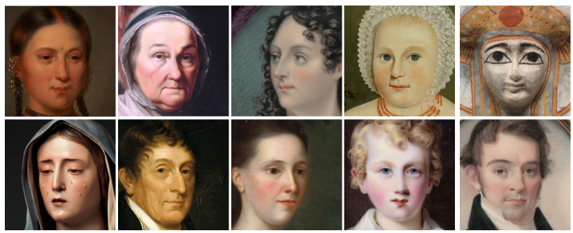
Figure 6:  Ground truth images from MetFaces dataset used for generating measurements.

Appendix H Additional experiments

H.1 Super-resolution

We present additional image super-resolution results for a more comprehensive understanding. Figure 7 illustrates the performance comparison of denoising and super-resolution using different priors. On the left side of Figure 7, the denoising performance of target (trained on MetFaces), mismatched (trained on BreCaHAD), adapted, and retrained priors is displayed. Meanwhile, on the right side, the reconstruction performance of target, mismatched, and adapted priors is presented. Note the improvement achieved by using adapted priors in both denoising and super-resolution tasks.

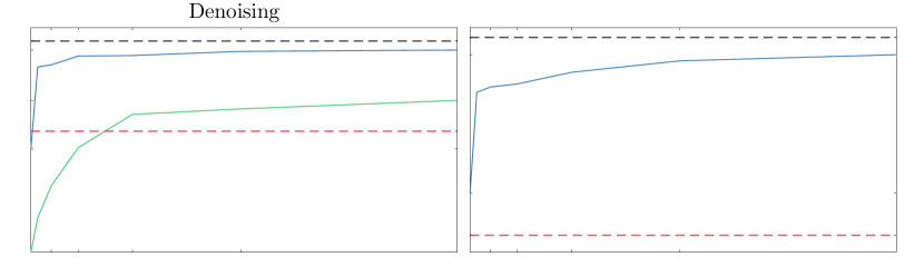
Figure 7:  The Left figure compares the empirical results of denoising for retrained and adapted priors vs. the number of training samples, as well as target (MetFaces) and mismatched (BreCaHAD) denoisers. The right figure compares PnP performance using target, mismatched, and adapted priors on super-resolution task. The results in both figures are reported for the test set from the MetFaces dataset, averaged for scaling factor of $s=4$. It’s worth highlighting the noticeable performance improvement of denoisers achieved through domain adaptation. Additionally, observe the relationship between PnP performance and adapted denoiser performance.

H.2 Deblurring

We present additional visual results for deblurring image restoration. Figure 8 presents a visual comparison of a test image from the MetFaces dataset using the target denoiser and four different mismatched denoisers. The images are convolved with the indicated blur kernel and subjected to Gaussian noise with a noise level of $v=0.01$. Note the suboptimal performance of mismatched priors in the deblurring task. As it is evident in Figure 8, the discrepancy between the mismatched distributions directly affects the PnP performance. Figure 9 illustrates a visual comparison of adapted priors in the deblurring task.

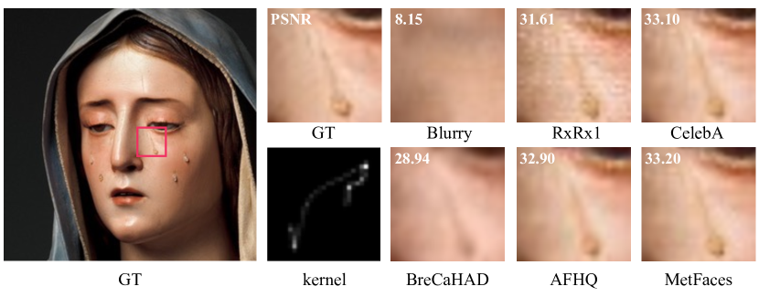
Figure 8:  Visual comparison of various mismatched denoisers for deblurring on an image from MetFaces dataset. The performance is reported in terms of PSNR (dB). The image is convolved with the indicated blur kernel and Gaussian noise with $v=0.01$ is added. Note that regardless of the PnP image restoration task, the discrepancies in training distributions result in mismatched priors and suboptimal performance in PnP.

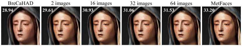
Figure 9:  Visual comparison of several adapted prior for image deblurring on a test image from MetFaces dataset. The performance is reported in terms of PSNR (dB). The experiment setting is similar to that of Figure 8. Note how adapting the mismatched prior with a larger set of data from the target distribution results in a better performance in PnP.

H.3 Various Distributions Experiment

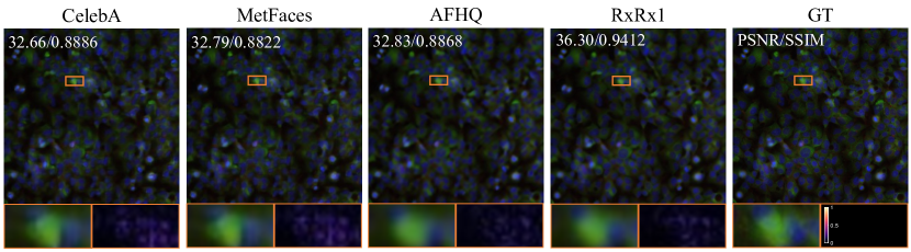
Figure 10:  Visual evaluation of several priors on the image super-resolution task reported in terms of PSNR (dB) and SSIM for an image from RxRx1. Images are downsampled with the scale of $s=4$ and convolved with the indicated blur kernel in Figure 3. Note the influence of mismatched priors on the performance of PnP.

We present additional visual results for mismatched priors and domain adaptation using various distributions for image super-resolution. In the following Figures, we demonstrate the effect of mismatched priors and prior adaptation tested on an images from RxRx1 [68] dataset. Figure 10 presents a visual comparison for PnP on super-resolution task using the target and three mismatched priors on an image from the RxRx1 test set. The images are convolved with the blur kernel indicted in Figure 3. Figure 11 illustrates visual results for domain adaptation of mismatched prior trained on CelebA dataset and adapted to RxRx1 distribution. Note the improvement in PnP performance by using adapted priors. Also, note the relation between PnP performance and the number of samples from the target distribution used for adaptation.

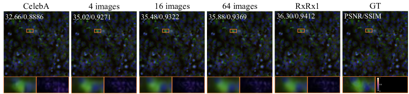
Figure 11:  Visual comparison of image super-resolution with target (RxRx1), mismatched (CelebA), and adapted priors on a test image from RxRx1. The images are downsampled by the scale of $s=4$. The performance is reported in terms of PSNR (dB) and SSIM. Note how the recovery performance increases by adaptation of mismatched priors to a larger set of images from the target distribution.

References

• [1] M. T. McCann, K. H. Jin, and M. Unser, “Convolutional neural networks for inverse problems in imaging: A review,” IEEE Signal Process. Mag., vol. 34, no. 6, pp. 85–95, 2017.
• [2] A. Lucas, M. Iliadis, R. Molina, and A. K. Katsaggelos, “Using deep neural networks for inverse problems in imaging: Beyond analytical methods,” IEEE Signal Process. Mag., vol. 35, no. 1, pp. 20–36, Jan. 2018.
• [3] G. Ongie, A. Jalal, C. A. Metzler, R. G. Baraniuk, A. G. Dimakis, and R. Willett, “Deep learning techniques for inverse problems in imaging,” IEEE J. Sel. Areas Inf. Theory, vol. 1, no. 1, pp. 39–56, May 2020.
• [4] S. V. Venkatakrishnan, C. A. Bouman, and B. Wohlberg, “Plug-and-play priors for model based reconstruction,” in Proc. IEEE Global Conf. Signal Process. and Inf. Process., Austin, TX, USA, Dec. 3-5, 2013, pp. 945–948.
• [5] S. Sreehari, S. V. Venkatakrishnan, B. Wohlberg, G. T. Buzzard, L. F. Drummy, J. P. Simmons, and C. A. Bouman, “Plug-and-play priors for bright field electron tomography and sparse interpolation,” IEEE Trans. Comput. Imaging, vol. 2, no. 4, pp. 408–423, Dec. 2016.
• [6] C. Metzler, P. Schniter, A. Veeraraghavan, and R. Baraniuk, “prDeep: Robust phase retrieval with a flexible deep network,” in Proc. 36th Int. Conf. Mach. Learn., Stockholmsmässan, Stockholm Sweden, Jul. 10–15 2018, pp. 3501–3510.
• [7] K. Zhang, W. Zuo, S. Gu, and L. Zhang, “Learning deep CNN denoiser prior for image restoration,” in Proc. IEEE Conf. Comput. Vis. and Pattern Recognit., Honolulu, USA, July 21-26, 2017, pp. 3929–3938.
• [8] T. Meinhardt, M. Moeller, C. Hazirbas, and D. Cremers, “Learning proximal operators: Using denoising networks for regularizing inverse imaging problems,” in Proc. IEEE Int. Conf. Comp. Vis., Venice, Italy, Oct. 22-29, 2017, pp. 1799–1808.
• [9] W. Dong, P. Wang, W. Yin, G. Shi, F. Wu, and X. Lu, “Denoising prior driven deep neural network for image restoration,” IEEE Trans. Pattern Anal. Mach. Intell., vol. 41, no. 10, pp. 2305–2318, Oct 2019.
• [10] K. Zhang, W. Zuo, and L. Zhang, “Deep plug-and-play super-resolution for arbitrary blur kernels,” in Proc. IEEE Conf. Comput. Vis. Pattern Recognit., Long Beach, CA, USA, June 16-20, 2019, pp. 1671–1681.
• [11] K. Wei, A. Aviles-Rivero, J. Liang, Y. Fu, C.-B. Schönlieb, and H. Huang, “Tuning-free plug-and-play proximal algorithm for inverse imaging problems,” in Proc. 37th Int. Conf. Mach. Learn., 2020.
• [12] K. Zhang, Y. Li, W. Zuo, L. Zhang, L. Van Gool, and R. Timofte, “Plug-and-play image restoration with deep denoiser prior,” IEEE Trans. Patt. Anal. and Machine Intell., pp. 1–1, 2021.
• [13] S. H. Chan, X. Wang, and O. A. Elgendy, “Plug-and-play ADMM for image restoration: Fixed-point convergence and applications,” IEEE Trans. Comp. Imag., vol. 3, no. 1, pp. 84–98, Mar. 2017.
• [14] Y. Romano, M. Elad, and P. Milanfar, “The little engine that could: Regularization by denoising (RED),” SIAM J. Imaging Sci., vol. 10, no. 4, pp. 1804–1844, 2017.
• [15] G. T. Buzzard, S. H. Chan, S. Sreehari, and C. A. Bouman, “Plug-and-play unplugged: Optimization free reconstruction using consensus equilibrium,” SIAM J. Imaging Sci., vol. 11, no. 3, pp. 2001–2020, Sep. 2018.
• [16] A. M. Teodoro, J. M. Bioucas-Dias, and M. A. T. Figueiredo, “A convergent image fusion algorithm using scene-adapted Gaussian-mixture-based denoising,” IEEE Trans. Image Process., vol. 28, no. 1, pp. 451–463, Jan. 2019.
• [17] R. Ahmad, C. A. Bouman, G. T. Buzzard, S. Chan, S. Liu, E. T. Reehorst, and P. Schniter, “Plug-and-play methods for magnetic resonance imaging: Using denoisers for image recovery,” IEEE Sig. Process. Mag., vol. 37, no. 1, pp. 105–116, 2020.
• [18] X. Yuan, Y. Liu, J. Suo, and Q. Dai, “Plug-and-play algorithms for large-scale snapshot compressive imaging,” in Proc. IEEE Conf. Comput. Vis. Pattern Recognit., 2020, pp. 1447–1457.
• [19] U. S. Kamilov, C. A. Bouman, G. T. Buzzard, and B. Wohlberg, “Plug-and-play methods for integrating physical and learned models in computational imaging: Theory, algorithms, and applications,” IEEE Signal Process. Mag., vol. 40, no. 1, pp. 85–97, 2023.
• [20] E. T. Reehorst and P. Schniter, “Regularization by denoising: Clarifications and new interpretations,” IEEE Trans. Comput. Imag., vol. 5, no. 1, pp. 52–67, Mar. 2019.
• [21] Y. Sun, B. Wohlberg, and U. S. Kamilov, “An online plug-and-play algorithm for regularized image reconstruction,” IEEE Trans. Comput. Imaging, vol. 5, no. 3, pp. 395–408, Sept. 2019.
• [22] Y. Sun, J. Liu, and U. S. Kamilov, “Block coordinate regularization by denoising,” in Proc. Adv. in Neural Inf. Process. Syst. 33, Vancouver, BC, Canada, Dec. 2019, pp. 382–392.
• [23] J. Liu, S. Asif, B. Wohlberg, and U. S. Kamilov, “Recovery analysis for plug-and-play priors using the restricted eigenvalue condition,” in Proc. Adv. Neural Inf. Process. Syst. 34, December 6-14, 2021, pp. 5921–5933.
• [24] Z. Kadkhodaie and E. Simoncelli, “Stochastic solutions for linear inverse problems using the prior implicit in a denoiser,” Proc. Adv. Neural Inf. Process. Syst., vol. 34, pp. 13242–13254, 2021.
• [25] R. Cohen, Y. Blau, D. Freedman, and E. Rivlin, “It has potential: Gradient-driven denoisers for convergent solutions to inverse problems,” in Proc. Adv. Neural Inf. Process. Syst. 34, 2021.
• [26] S. Hurault, A. Leclaire, and N. Papadakis, “Gradient step denoiser for convergent plug-and-play,” in Int. Conf. on Learn. Represent., Kigali, Rwanda, May 1-5, 2022.
• [27] R. Laumont, V. De Bortoli, A. Almansa, J. Delon, A. Durmus, and M. Pereyra, “Bayesian imaging using plug & play priors: When Langevin meets Tweedie,” SIAM J. Imaging Sci., vol. 15, no. 2, pp. 701–737, 2022.
• [28] Y. Sun, Z. Wu, B. Wohlberg, and U. S. Kamilov, “Scalable plug-and-play ADMM with convergence guarantees,” IEEE Trans. Comput. Imag., vol. 7, pp. 849–863, July 2021.
• [29] J. Tang and M. Davies, “A fast stochastic plug-and-play ADMM for imaging inverse problems,” arXiv:2006.11630, 2020.
• [30] R. G. Gavaskar and K. N. Chaudhury, “On the proof of fixed-point convergence for plug-and-play admm,” IEEE Signal Process. Lett., vol. 26, no. 12, pp. 1817–1821, 2019.
• [31] S. H. Chan, “Performance analysis of plug-and-play admm: A graph signal processing perspective,” IEEE Trans. Comp. Imag., vol. 5, no. 2, pp. 274–286, June 2019.
• [32] E. K. Ryu, J. Liu, S. Wang, X. Chen, Z. Wang, and W. Yin, “Plug-and-play methods provably converge with properly trained denoisers,” in Proc. 36th Int. Conf. Mach. Learn., Long Beach, CA, USA, Jun. 09–15 2019, vol. 97, pp. 5546–5557.
• [33] L. I. Rudin, S. Osher, and E. Fatemi, “Nonlinear total variation based noise removal algorithms,” Physica D, vol. 60, no. 1–4, pp. 259–268, Nov. 1992.
• [34] A. Beck and M. Teboulle, “Fast gradient-based algorithm for constrained total variation image denoising and deblurring problems,” IEEE Trans. Image Process., vol. 18, no. 11, pp. 2419–2434, November 2009.
• [35] Z. Wang, D. Liu, J. Yang, W. Han, and T. Huang, “Deep networks for image super-resolution with sparse prior,” in Proc. IEEE Int. Conf. Comp. Vis., Santiago, Chile, December 13-16, 2015, pp. 370–378.
• [36] D. Jin, R. Zhou, Z. Yaqoob, and P. So, “Tomographic phase microscopy: Principles and applications in bioimaging,” J. Opt. Soc. Am. B, vol. 34, no. 5, pp. B64–B77, 2017.
• [37] E. Kang, J. Min, and J. C. Ye, “A deep convolutional neural network using directional wavelets for low-dose x-ray CT reconstruction,” Med. Phys., vol. 44, no. 10, pp. e360–e375, 2017.
• [38] A. Zafari, A. Khoshkhahtinat, P. Mehta, M. S. E. Saadabadi, M. Akyash, and N. M. Nasrabadi, “Frequency disentangled features in neural image compression,” arXiv:2308.02620, 2023.
• [39] H. Chen, Y. Zhang, M. K. Kalra, F. Lin, Y. Chen, P. Liao, J. Zhou, and G. Wang, “Low-dose CT with a residual encoder-decoder convolutional neural network,” IEEE Trans. Med. Imag., vol. 36, no. 12, pp. 2524–2535, Dec. 2017.
• [40] X. Xu and U. S. Kamilov, “Signprox: One-bit proximal algorithm for nonconvex stochastic optimization,” in IEEE Int. Conf. Acoustics, Speech and Signal Process., Brighton, UK, May 2019, pp. 7800–7804.
• [41] V. Monga, Y. Li, and Y. C. Eldar, “Algorithm unrolling: Interpretable, efficient deep learning for signal and image processing,” IEEE Signal Process. Mag., vol. 38, no. 2, pp. 18–44, Mar. 2021.
• [42] J. Zhang and B. Ghanem, “ISTA-Net: Interpretable optimization-inspired deep network for image compressive sensing,” in Proc. IEEE Conf. Comput. Vision Pattern Recognit., 2018, pp. 1828–1837.
• [43] A. Hauptmann, F. Lucka, M. Betcke, N. Huynh, J. Adler, B. Cox, P. Beard, S. Ourselin, and S. Arridge, “Model-based learning for accelerated, limited-view 3-d photoacoustic tomography,” IEEE Trans. Med. Imag., vol. 37, no. 6, pp. 1382–1393, 2018.
• [44] D. Gilton, G. Ongie, and R. Willett, “Deep equilibrium architectures for inverse problems in imaging,” IEEE Trans. Comput. Imag., vol. 7, pp. 1123–1133, 2021.
• [45] J. Liu, X. Xu, W. Gan, S. Shoushtari, and U. S. Kamilov, “Online deep equilibrium learning for regularization by denoising,” in Proc. Adv. Neural Inf. Process. Syst., New Orleans, LA, 2022.
• [46] T. Tirer and R. Giryes, “Image restoration by iterative denoising and backward projections,” IEEE Trans. Image Process., vol. 28, no. 3, pp. 1220–1234, Mar. 2019.
• [47] M. Terris, A. Repetti, and Y. Pesquet, J. C.and Wiaux, “Building firmly nonexpansive convolutional neural networks,” in IEEE Int. Conf. Acoustics, Speech and Signal Process., 2020, pp. 8658–8662.
• [48] J. Hertrich, S. Neumayer, and G. Steidl, “Convolutional proximal neural networks and plug-and-play algorithms,” Linear Algebra and its Appl., vol. 631, pp. 203–234, 2021.
• [49] P. Bohra, D. Perdios, A. Goujon, S. Emery, and M. Unser, “Learning lipschitz-controlled activation functions in neural networks for plug-and-play image reconstruction methods,” in NeurIPS 2021 Workshop on Deep Learning and Inverse Problems, 2021.
• [50] X. Xu, Y. Sun, J. Liu, B. Wohlberg, and U. S. Kamilov, “Provable convergence of plug-and-play priors with mmse denoisers,” IEEE Signal Process. Lett., vol. 27, pp. 1280–1284, 2020.
• [51] R. Gribonval, “Should penalized least squares regression be interpreted as maximum a posteriori estimation?,” IEEE Trans. Signal Process., vol. 59, no. 5, pp. 2405–2410, May 2011.
• [52] S. Hurault, A. Leclaire, and N. Papadakis, “Proximal denoiser for convergent plug-and-play optimization with nonconvex regularization,” in Int. Conf. Mach. Learn. PMLR, 2022, pp. 9483–9505.
• [53] S. Boyd, N. Parikh, E. Chu, B. Peleato, and J. Eckstein, “Distributed optimization and statistical learning via the alternating direction method of multipliers,” Foundations and Trends in Machine Learning, vol. 3, no. 1, pp. 1–122, July 2011.
• [54] Y. Sun, X. Wang, Z. Liu, J. Miller, A. Efros, and M. Hardt, “Test-time training with self-supervision for generalization under distribution shifts,” in Int. Conf. Mach. Learn. PMLR, 2020, pp. 9229–9248.
• [55] M. Z. Darestani, A. S. Chaudhari, and R. Heckel, “Measuring robustness in deep learning based compressive sensing,” in Proc. 38th Int. Conf. Machine Learning (ICML), July 18-24, 2021, pp. 2433–2444.
• [56] M. Z. Darestani, J. Liu, and R. Heckel, “Test-time training can close the natural distribution shift performance gap in deep learning based compressed sensing,” in Proc. 39th Int. Conf. Machine Learning (ICML), Baltimore, MD, USA, Jul 17-23, 2022, pp. 4754–4776.
• [57] A. Jalal, M. Arvinte, G. Daras, E. Price, A. G. Dimakis, and J. Tamir, “Robust compressed sensing MRI with deep generative priors,” in Proc. Adv. Neural Inf. Process. Syst. 34, Dec 6-14, 2021, pp. 14938–14954.
• [58] S. Shoushtari, J. Liu, Y. Hu, and U. S. Kamilov, “Deep model-based architectures for inverse problems under mismatched priors,” IEEE J. Sel. Areas in Inf. Theory, vol. 3, no. 3, pp. 468–480, 2022.
• [59] J. Liu, Y. Sun, C. Eldeniz, W. Gan, H. An, and U. S. Kamilov, “RARE: Image reconstruction using deep priors learned without ground truth,” IEEE J. Sel. Topics Signal Process., vol. 14, no. 6, pp. 1088–1099, Oct. 2020.
• [60] S. A. Bigdeli, M. Zwicker, P. Favaro, and M. Jin, “Deep mean-shift priors for image restoration,” Proc. Adv. Neural Inf. Process. Syst., vol. 30, 2017.
• [61] W. Gan, S. Shoushtari, Y. Hu, J. Liu, H. An, and U. S Kamilov, “Block coordinate plug-and-play methods for blind inverse problems,” arXiv:2305.12672, 2023.
• [62] Z. Li and J. Li, “A simple proximal stochastic gradient method for nonsmooth nonconvex optimization,” Adv. in Neural Inf. Process. Syst., vol. 31, 2018.
• [63] B. Jiang, T. Lin, S. Ma, and S. Zhang, “Structured nonconvex and nonsmooth optimization: algorithms and iteration complexity analysis,” Comput. Optim. and Appl., vol. 72, no. 1, pp. 115–157, 2019.
• [64] M. Yashtini, “Multi-block nonconvex nonsmooth proximal admm: Convergence and rates under kurdyka–łojasiewicz property,” Journal of Optim. Theory and Appl., vol. 190, no. 3, pp. 966–998, 2021.
• [65] T. Karras, M. Aittala, J. Hellsten, S. Laine, J. Lehtinen, and T. Aila, “Training generative adversarial networks with limited data,” Proc. Adv. Neural Inf. Process. Syst., vol. 33, pp. 12104–12114, 2020.
• [66] Z. Liu, P. Luo, X. Wang, and X. Tang, “Deep learning face attributes in the wild,” in Proc. IEEE. Int. Conf. Comp. Vis., December 2015.
• [67] Y. Choi, Y. Uh, J. Yoo, and J. Ha, “Stargan v2: Diverse image synthesis for multiple domains,” in Proc. IEEE Conf. Comput. Vis. and Pattern Recognit. (CVPR), 2020, pp. 8188–8197.
• [68] M. Sypetkowski, M. Rezanejad, S. Saberian, O. Kraus, J. Urbanik, J. Taylor, B. Mabey, M. Victors, J. Yosinski, A. Rezazadeh Sereshkeh, et al., “Rxrx1: A dataset for evaluating experimental batch correction methods,” in In Proc. IEEE Conf. Comput. Vis. Pattern Recognit, 2023, pp. 4284–4293.
• [69] A. Aksac, D. J. Demetrick, T. Ozyer, and R. Alhajj, “Brecahad: a dataset for breast cancer histopathological annotation and diagnosis,” BMC research notes, vol. 12, no. 1, pp. 1–3, 2019.
• [70] N. Zhao, Q. Wei, A. Basarab, N. Dobigeon, D. Kouamé, and J .Y. Tourneret, “Fast single image super-resolution using a new analytical solution for l2-l2 problems.,” IEEE Trans. Imag. Process., 2016.
• [71] R. Gribonval and P. Machart, “Reconciling “priors” & “priors” without prejudice?,” in Proc. Adv. Neural Inf. Process. Syst. 26, Lake Tahoe, NV, USA, December 5-10, 2013, pp. 2193–2201.
• [72] A. Kazerouni, U. S. Kamilov, E. Bostan, and M. Unser, “Bayesian denoising: From MAP to MMSE using consistent cycle spinning,” IEEE Signal Process. Lett., vol. 20, no. 3, pp. 249–252, March 2013.
• [73] R. Gribonval and M. Nikolova, “On Bayesian estimation and proximity operators,” Appl. Comput. Harmon. Anal., vol. 50, pp. 49–72, Jan. 2021.
• [74] Y. Sun, S. Xu, Y. Li, L. Tian, B. Wohlberg, and U. S. Kamilov, “Regularized Fourier ptychography using an online plug-and-play algorithm,” in Proc. IEEE Int. Conf. Acoustics, Speech and Signal Process. (ICASSP), Brighton, UK, May 12-17, 2019, pp. 7665–7669.
• [75] D. Kingma and J. Ba, “Adam: A method for stochastic optimization,” in Proc. Int. Conf. on Learn. Represent., 2015.