Event-Triggered Control of Neuron Growth
with Dirichlet Actuation at Soma

Abstract

We introduce a dynamic event-triggering mechanism for regulating the axonal growth of a neuron. We apply boundary actuation at the soma (the part of a neuron that contains the nucleus) and regulate the dynamics of tubulin concentration and axon length. The control law is formulated by applying a Zero-Order Hold (ZOH) to a continuous-time controller which guides the axon to reach the desired length. The proposed dynamic event-triggering mechanism determines the specific time instants at which control inputs are sampled from the continuous-time control law. We establish the existence of a minimum dwell-time between two triggering times that ensures avoidance of Zeno behavior. Through employing the Lyapunov analysis with PDE backstepping, we prove the local stability of the closed-loop system in $\mathcal{H}_{1}$-norm, initially for the target system, and subsequently for the original system. The effectiveness of the proposed method is showcased through numerical simulations.

I Introduction

Recent advancements in neuroscience draw from various disciplines such as mathematics, physics, and engineering [17, 16, 19]. These fields are crucial for understanding the structure and functioning of neurons in the nervous system and addressing neurological issues. One major challenge in this context is the growth of axons, which are similar to wires and are constructed through the assembly of tubulin proteins. Axons function as connectors between neurons for transmitting electrical signals. Some neurological diseases, such as Alzheimer’s disease [27] and spinal cord injuries [26], can damage axons by impeding the assembly process of tubulin proteins, leading to halted growth or degeneration. Researchers are developing new therapies to treat these diseases. One promising therapy is called ChABC which involves injecting a bacterial enzyme that digests the axon growth inhibitors [2]. Following this therapy, axon growth can be sustained [18]. However, it’s important to note that ChABC has a limitation: ChABC requires repeated injections of the bacterial enzyme since it rapidly loses its activity at $37$^∘C [25]. To enhance the effectiveness of this therapy, the amount of enzymes required to achieve the desired axon length and the intervals for these repeated injections must be identified.

Studying the behavior of tubulin proteins can help achieve the desired axon length. For this reason, numerous mathematical models have employed Ordinary Differential Equations (ODEs) and Partial Differential Equations (PDEs) to clarify tubulin behavior [36, 28, 29]. Authors of [7] model the axon growth process as a coupled PDE-ODE with a moving boundary, akin to the Stefan problem, effectively describing the associated physical phenomena. In this model, the PDE represents tubulin concentration’s evolution along the axon, and the ODEs describe both the evolution of axon length and tubulin concentration at the growth cone. Given that this model captures this critical information about axon growth, it is worthwhile to consider designing a controller to regulate tubulin concentration and axon length. Over the past two decades, researchers have developed a technique. known as boundary control of PDE systems by PDE backstepping, to regulate PDEs by defining control laws at their boundaries [24]. Following the development of this technique, boundary control was expanded to the class of coupled PDE-ODE systems [23, 34, 35]. While the majority of these contributions are typically assumed to have a constant domain size over time, some researchers focused on a moving domain over time specifically addressing the Stefan problem, as discussed in [30, 8, 15]. Besides these studies, backstepping-based control techniques are constructed for Stefan problem in [22] with global stability results. Following this progress, several works have proposed local stability results for nonlinear hyperbolic PDEs, as seen in [3, 37]. We achieved local stability results for the first time for nonlinear parabolic PDEs with a moving boundary for the axon growth problem in our previous works [4, 6], and with input delay in [5].

While the control designs mentioned above operate in continuous time, certain technologies necessitate the performance of control actions only when necessary due to constraints on energy, communication, and computation [13]. To deal with this problem, an event-triggered control strategy is proposed for PID controllers in [1], and for state feedback and output feedback controllers for linear and nonlinear time-invariant systems in [14] and [20]. Authors of [31] ensured asymptotic stability for a closed-loop system with state feedback control laws by employing an event-triggering mechanism, characterizing it as a hybrid system. This characterization eased the constraints associated with the event-triggering mechanism and this relaxation is detailed in [12] as a dynamic triggering approach. In addition to its application in ODE systems, the authors of [9] successfully applied an event-triggered mechanism to boundary control hyperbolic PDE systems. This innovative approach paved the way for the utilization of event-triggered boundary control in reaction-diffusion PDEs as demonstrated in [10]. For Stefan problem, both static and dynamic event-triggered boundary control laws were developed by the authors of [32] and [33]. Furthermore, an event-triggering mechanism was employed to transition between safety utilizing CBFs and stability for Stefan problem with actuator dynamics as discussed in [21]. In this paper, we introduce a novel dynamic event-triggering mechanism for the axon growth problem which consists of a coupled reaction-diffusion-advection PDE and nonlinear ODEs with a moving boundary. With this dynamic event-triggering mechanism, we aim to address the key question around appropriate time intervals for administering therapy.

The contributions of this paper include (i) designing a control law for neuron growth with Dirichlet boundary actuation, (ii) developing a dynamic event-triggering mechanism for coupled reaction-diffusion-advection PDEs and nonlinear ODEs with a moving boundary, (iii) analyzing Zeno behavior avoidance, (iv) demonstrating local stability for the closed-loop system. Indeed, this work is pioneering in event-triggering boundary control for axon growth and marks the first local stability analysis using event-triggering mechanisms for PDE systems.

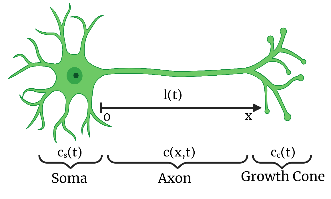
Figure 1: Schematic of neuron and state variables

II Modeling of Axon Growth

In this section, we present the mathematical model governing axon growth. This model includes a coupled system of PDEs and ODEs, featuring a dynamic boundary that describes tubulin behavior along the axon and axon growth. We also introduce the steady-state solution for a target axon length and a reference error system.

II-A Axon growth model by a moving boundary PDE

The evolution of tubulin along the axon serves as the primary catalyst for the axon growth process, and to understand this process, we rely on two assumptions to create a mathematical model which are described in our previous work [4]. Thus, the axonal growth can be modeled as

$$c_{t}(x,t)= Dc_{xx}(x,t)-ac_{x}(x,t)-gc(x,t),$$ (1)

$$c(0,t)= -q_{\rm s}(t),$$ (2)

$$c(l(t),t)= c_{\rm c}(t),$$ (3)

$$l_{\rm c}\dot{c}_{\rm c}(t)= (a-gl_{\rm c})c_{\rm c}(t)-Dc_{x}(l(t),t)$$

$$-(r_{\rm g}c_{\rm c}(t)+\tilde{r}_{\rm g}l_{\rm c})(c_{\rm c}(t)-c_{\infty}),$$ (4)

$$\dot{l}(t)= r_{\rm g}(c_{c}(t)-c_{\infty}),$$ (5)

In this model, the PDE state $c(x,t)$ represents tubulin concentration within the axon. ODE states include $c_{\rm c}(t)$ for tubulin concentration in the growth cone, $l(t)$ for axon length, and $q_{\rm s}(t)$ for tubulin concentration in the soma. Tubulin proteins move along the axon at a rate $a$ and degrade at a constant rate $g$. The diffusivity constant in (1) is represented by $D$. Axonal growth stops when the tubulin concentration in the cone reaches equilibrium, denoted as $c_{\infty}$. The other parameters in this model are explained with details in our previous work [4] and [6].

II-B Steady-state solution

For a desired axon length, $l_{s}$, we first derive a steady-state solution of the concentration. The steady-state solution of (1)-(5) is obtained as follows

$$c_{\rm eq}(x)=c_{\infty}\left(K_{+}e^{\lambda_{+}(x-l_{\rm s})}+K_{-}e^{\lambda_{-}(x-l_{\rm s})}\right),$$ (6)

where

$$\lambda_{+}= \frac{a}{2D}+\frac{\sqrt{a^{2}+4Dg}}{2D},\ \lambda_{-}=\frac{a}{2D}-\frac{\sqrt{a^{2}+4Dg}}{2D},$$ (7)

$$K_{+}= \frac{1}{2}+\frac{a-2gl_{\rm c}}{2\sqrt{a^{2}+4Dg}},\quad K_{-}=\frac{1}{2}-\frac{a-2gl_{\rm c}}{2\sqrt{a^{2}+4Dg}}.$$ (8)

We obtain the steady-state input for the concentration in the soma as

$$q_{\rm s}^{*}=-c_{\infty}\left(K_{+}e^{-\lambda_{+}l_{\rm s}}+K_{-}e^{-\lambda_{-}l_{\rm s}}\right).$$ (9)

II-C Reference error system

Let us consider the following reference error states

$$u(x,t)=c(x,t) -c_{\rm eq}(x),$$ (10)

$$z_{1}(t)=c_{\rm c}(t)-c_{\infty} ,\quad z_{2}(t)=l(t)-l_{\rm s},$$ (11)

$$U(t)=-(q_{\rm s} (t)-q_{\rm s}^{*}).$$ (12)

where $U(t)$ is the reference error input. Utilizing (10)-(12), (6) and (9) in the governing equations (1)-(5), we derive the reference error system as

$$u_{t}(x,t)= Du_{xx}(x,t)-au_{x}(x,t)-gu(x,t),$$ (13)

$$u(0,t)= U(t),$$ (14)

$$u(l(t),t)= c_{\rm c}(t)-c_{\rm eq}(l(t)),$$ (15)

$$\dot{z}_{1}(t)= \tilde{a}_{1}z_{1}(t)-\beta u_{x}(l(t),t)-\kappa z_{1}(t)^{2}+\beta f_{1}(z_{2}(t))$$

$$-\beta\tilde{a}_{2}z_{2}(t),$$ (16)

$$\dot{z}_{2}(t)= r_{\rm g}z_{1}(t),$$ (17)

where the constants in (13)-(17) are

$$\tilde{a}_{1} =\frac{a-r_{\rm g}c_{\infty}}{l_{\rm c}}-g-\tilde{r}_{\rm g},\quad\beta=\frac{D}{l_{\rm c}},$$ (18)

$$\tilde{a}_{2} =c_{\infty}\left(\lambda_{+}^{2}K_{+}+\lambda_{-}^{2}K_{-}\right),\quad\kappa=\frac{r_{\rm g}}{l_{\rm c}},$$ (19)

$$f_{1}(z_{2}(t))= -c_{\infty}\left(K_{+}\lambda_{+}e^{\lambda_{+}z_{2}(t)}+K_{-}\lambda_{-}e^{\lambda_{-}z_{2}(t)}\right)$$

$$+\tilde{a}_{2}z_{2}(t)+c_{\infty}\frac{a-gl_{\rm c}}{D}.$$ (20)

The ODEs can be written using the state vector $X(t)\in\mathbb{R}^{2}$ as $X(t)=[z_{1}(t)\quad z_{2}(t)]^{\top}$. The system (15)–(17) simplifies

$$u_{t}(x,t)= Du_{xx}(x,t)-au_{x}(x,t)-gu(x,t),$$ (21)

$$u(0,t)= U(t),$$ (22)

$$u(l(t),t)= h(X(t)),$$ (23)

$$\dot{X}(t)= AX(t)+f(X(t))+Bu_{x}(l(t),t),$$ (24)

where

$$A= \left[\begin{array}[]{cc}\tilde{a}&-\beta\tilde{a}_{2}\\ r_{\rm g}&0\end{array}\right],\quad B=\left[\begin{array}[]{c}-\beta\\ 0\end{array}\right],$$ (29)

$$f(X(t))= -\kappa z_{1}(t)^{2}+\beta f_{1}(z_{2}(t)),$$ (30)

$$h(X(t))= e_{1}X(t)+\tilde{h}(e_{2}X(t)),$$ (31)

$$\tilde{h}(z_{2}(t))= c_{\infty}\left(1-K_{+}e^{\lambda_{+}z_{2}(t)}-K_{-}e^{\lambda_{-}z_{2}(t)}\right).$$ (32)

III Continous-time and Sample-based Control Design

First, we linearize nonlinear ODEs in (24) around zero states as

$$u_{t}(x,t)= Du_{xx}(x,t)-au(x,t)-gu(x,t),$$ (33)

$$u_{x}(0,t)= U(t),$$ (34)

$$u(l(t),t)= H^{\top}X(t),$$ (35)

$$\dot{X}(t)= A_{1}X(t)+Bu_{x}(l(t),t),$$ (36)

where the vector $H\in\mathbb{R}^{2}$ is defined as

$$A_{1} =\left[\begin{array}[]{cc}\tilde{a}_{1}&\tilde{a}_{3}\\ r_{\rm g}&0\end{array}\right],\color[rgb]{0,0,0}~{}H=\left[1\quad-\frac{(a-gl_{\rm c})c_{\infty}}{D}\right]^{\top},$$ (39)

where $\tilde{a}_{3}=\frac{a^{2}+Dg-agl_{\rm c}}{D^{2}}$.

In this paper, our continuous-time control design relies on a backstepping transformation, as outlined in [4]. This transformation maps the linear reference error system $(u,X)$ to a corresponding nonlinear target system $(w,X)$ by utilizing the following backstepping transformation.

$$w(x,t)= u(x,t)-\int_{x}^{l(t)}k(x,y)u(y,t)dy$$

$$-\phi(x-l(t))^{\top}X(t),$$ (40)

$$u(x,t)= w(x,t)+\int_{x}^{l(t)}q(x,y)w(y,t)dy$$

$$+\varphi(x-l(t))^{\top}X(t),$$ (41)

where $k(x,y)\in\mathbb{R}$ and $\phi(x-l(t))\in\mathbb{R}^{2}$ are the gain kernel functions are explicitly described in [4]. We suppose the desired target system as

$$w_{t}(x,t)= Dw_{xx}(x,t)-aw_{x}(x,t)-gw(x,t)$$

$$-\dot{l}(t)F(x,X(t)),$$ (42)

$$w(0,t)= 0,$$ (43)

$$w(l(t),t)= 0,$$ (44)

$$\dot{X}(t)= (A_{1}+BK^{\top})X(t)+Bw_{x}(l(t),t),$$ (45)

and $K\in\mathbb{R}^{2}$ is chosen to ensure the stability of $A+BK$ such that it is Hurwitz, satisfying

$$k_{1}>\frac{\tilde{a}_{1}}{\beta},\quad k_{2}>\frac{\tilde{a}_{3}}{\beta}.$$ (46)

Furthermore, we describe the redundant nonlinear term $F(x,X(t))\in\mathbb{R}$ in (III), arising from the moving boundary, as $F(x,X(t))=\left(\phi^{\prime}(x-l(t))^{T}-k(x,l(t))C^{T}\right)X(t)$.

III-A Control law

The continuous-time control law is obtained based on the boundary condition (43) of the target system at $x=0$, utilizing the gain kernel solutions as detailed in [4].

$$\phi(x)^{\top}= \begin{bmatrix}H^{\top}&K^{\top}-\frac{1}{D}H^{\top}BH^{\top}\end{bmatrix}e^{N_{1}x}\begin{bmatrix}I\\ 0\end{bmatrix},$$ (47)

$$k(x,y)= -\frac{1}{D}\phi(x-y)^{\top}B,$$ (48)

where $N_{1}$ is defined in equation (37) in [4]. Substituting $x=0$ into the transformation (III), we have the control law as

$$U(t)=\int_{0}^{l(t)}k(0,y)u(y,t)dx+\phi(-l(t))X(t),$$ (49)

It is worth noting that the solutions of the inverse gain kernels $q(x,y)$ and $\varphi(x)$ can be found in [4]. This invertibility of the backstepping transformation is essential for demonstrating the stability of the $(u,X)$-system.

III-B Sample-based control law

We aim to stabilize the closed-loop system (1)-(5) by using sampling for the continuous-time controller defined in (49) with the increasing sequence of time $(t_{j})_{j\in\mathbb{N}}$. Thus, the control input is given by

$$U(t_{j})= \int_{0}^{l(t_{j})}k(0,x)u(x,t_{j})dx+\phi(-l(t_{j}))X(t_{j}).$$ (50)

which means that the boundary condition (14) is modified as

$$u(0,t)=U(t_{j}).$$ (51)

Now, the reference error system can be written as

$$u_{t}(x,t)= Du_{xx}(x,t)-au_{x}(x,t)-gu(x,t),$$ (52)

$$u(0,t)= U(t_{j}),$$ (53)

$$u(l(t),t)= h(X(t)),$$ (54)

$$\dot{X}(t)= AX(t)+f(X(t))+Bu_{x}(l(t)t).$$ (55)

To establish stability results, we transform the reference error system in (52)-(55) to the target system using the transformation in (III). Thus, the target system is

$$w_{t} (x,t)=Dw_{xx}(x,t)-aw_{x}(x,t)-gw(x,t)$$

$$-\dot{l}(t)\left(k(x,l(t))u(l(t),t)-\phi^{\prime}(x-l(t))^{T}X(t)\right)$$

$$-\phi(x-l(t))^{\top}f(X(t))$$

$$-\left(\phi^{\prime}(x-l(t))^{\top}B+\frac{a}{D}\phi(x-l(t))^{\top}B\right)h^{*}(X),$$ (56)

$$w (0,t)=d(t),$$ (57)

$$w (l(t),t)=h^{*}(X(t)),$$ (58)

$$\dot{X} (t)=(A+BK)X(t)+f(X(t))+Bw_{x}(l(t),t),$$ (59)

where

$$h^{*}(X(t))=\left(z_{1}(t)+\tilde{h}(z_{2}(t))\right)-H^{\top}X(t).$$ (60)

and the error between continuous-time control law in (49) and sample-based control law in (50) is defined as

$$d(t)=U(t)-U(t_{j}).$$ (61)

IV Event-triggered based boundary control

In this section, we introduce the event-triggered state-feedback control approach, deriving sampling times for our control law to obtain the event-triggering mechanism.

Definition 1.

The design parameters are $\gamma>0$, $\eta>0$, $\rho>0$ and $\beta_{i}>0$ where $i\in\{1,...5\}$. The event-based controller consists of two trigger mechanisms:

1. The event-trigger: The set of all event times are in increasing sequence and they are denoted as $I=\{t_{0},t_{1},...\}$ where $t_{0}=0$ with the following rule

   • If $S(t,t_{j})=\emptyset$, then the set of the times of the events is $\{t_{0},...,t_{j}\}$.

   • If $S(t,t_{j})\neq\emptyset$, the next event time is $t_{j+1}=\inf\left(S(t,t_{j})\right)$ where

     $$S(t,t_{j})=\{t\in\mathbb{R}_{+}|t>t_{j}\wedge d^{2}(t)>-\gamma m(t)\}$$ (62)

     for all $t\in[t_{j},t_{j+1})$, $d(t)$ is given by (61) and $m(t)$ satisfies the ODE

     $$\dot{m}(t)= -\eta m(t)+\rho d(t)^{2}-\beta_{1}X(t)^{2}-\beta_{2}X(t)^{4}$$

     $$-\beta_{3}|w_{x}(0,t)|^{2}-\beta_{4}||w(x,t))||^{2}$$

     $$-\beta_{5}|w_{x}(l(t),t)|^{2}.$$ (63)

2. The control action: The feedback control law that is derived in (50) for all $t\in[t_{j},t_{j+1})$ where $j\in\mathbb{N}$.

Lemma 1.

Under the definition of the state feedback event-triggered boundary control, it holds that $d^{2}(t)\leq-\gamma m(t)$ and $m(t)>0$ for $t\in[0,F)$, where $F=\sup(I)$.

Proof.

From the definition of the event-trigger approach, it is guaranteed that $d^{2}(t)\leq-\gamma m(t)$, $t\in[0,F)$/ It yields

$$\dot{m}(t) \leq-(\eta+\gamma\rho)m(t)-\beta_{1}X^{2}(t)-\beta_{2}X^{4}(t)$$

$$-\beta_{3}w_{x}(0,t)^{2}-\beta_{4}||w(x,t)||^{2}-\beta_{5}w_{x}(l(t),t)^{2}$$ (64)

for $t\in(t_{j},t_{j+1}),~{}j\in\mathbb{N}$. Considering time continuity of $m(t)$, we can obtain

$$m(t)\leq m(t_{j})e^{-(\eta+\rho\sigma)(t-t_{j})}$$

$$-\int_{t_{j}}^{t}e^{-(\eta+\rho\sigma)(t-\tau)}\left(\beta_{1}X(\tau)^{2}+\beta_{2}X(\tau)^{4}\right)d\tau$$

$$-\int_{t_{j}}^{t}e^{-(\eta+\rho\sigma)(t-\tau)}(\beta_{3}|u_{x}(0,\tau)|^{2}d\tau+\beta_{5}|u_{x}(l(\tau),\tau)|^{2})$$

$$-\int_{t_{j}}^{t}e^{-(\eta+\rho\sigma)(t-\tau)}\beta_{4}||u(x,\tau))||^{2}$$ (65)

From the event-trigger mechanism definition, we have that $m(t_{0})=m(0)<0$. Therefore, the estimate of $m(t)$ in (65) ensures that $m(t)<0$ for all $t\in[0,t_{1}]$. This can be generalized for all $t$. which means it can be shown that $m(t)<0$ for $t\in[0,F)$. ∎

Lemma 2.

For $d(t)$ , it holds that

$$(\dot{d}(t))^{2}\leq \rho_{1}d^{2}(t)+\alpha_{1}X(t)^{2}+\alpha_{2}X(t)^{4}+\alpha_{3}w_{x}(0,t)^{2}$$

$$+\alpha_{4}||w(x,t)||^{2}+\alpha_{5}w_{x}(l(t),t)^{2}$$ (66)

for some positive constants $\rho_{1},~{}\alpha_{1},~{}\alpha_{2},~{}\alpha_{3},~{}\alpha_{4}$ and $\alpha_{5}$ for all $t\in(t_{j},t_{j+1})$, $j\in\mathbb{N}$.

Proof.

By taking the time derivative of (61) and (50), along with the system (52)–(55) we get

$$\dot{d}(t)= \left(\dot{\phi}(0)B+\frac{1}{D}H^{\top}B\right)d(t)+H^{\top}Bu_{x}(0,t)$$

$$+\left(Dk(0,l(t))+\phi(l(t))B\right)u_{x}(l(t),t)$$

$$+\int_{0}^{l(t)}\left(Dk_{yy}(0,y)+ak_{y}(0,y)\right)u(y,t)dy$$

$$-\int_{0}^{l(t)}\left(g+\dot{\phi}(0)B+\frac{1}{D}H^{\top}B\right)k(0,y)u(y,t)dy$$

$$-\dot{l}(t)\dot{\phi}(-l(t))X(t)+\phi(-l(t))f(X(t))$$

$$+\left(\phi(-l(t))^{\top}B-ak(0,l(t))\right)u(l(t),t)$$

$$-\left(\dot{\phi}(0)B+\frac{1}{D}H^{\top}B-A\right)\phi(-l(t))X(t)$$

$$+\dot{l}(t)h(X(t))k(0,l(t))$$ (67)

By using inverse transformation of backstepping in (41), Young’s and Cauchy Schwarz’s inequalities, one can show

$$||u||^{2}\leq \left(\frac{3}{2}+\frac{3}{2}\left(\int_{0}^{l(t)}\int_{x}^{l(t)}q(x,y)^{2}dydx\right)^{1/2}\right)^{2}||w||^{2}$$

$$+\frac{3}{2}\left(\int_{0}^{l(t)}\varphi(x-l(t))^{\top}dx\right)^{2}X(t)^{2}$$ (68)

Applying the same procedure, we can also demonstrate that

$$u(l(t),t)^{2}\leq 2w(l(t),t)^{2}+2(\varphi(0)^{\top})^{2}X(t)^{2},$$ (69)

$$u_{x}(0,t)^{2}\leq 4w_{x}(0,t)^{2}+4q(0,0)^{2}w(0,t)^{2}$$

$$+4\int_{0}^{l(t)}q_{x}(0,y)^{2}dy||w(y,t)||^{2}$$

$$+4(\varphi(-l(t))^{\top})^{2}X(t)^{2},$$ (70)

$$u_{x}(l(t),t)^{2}\leq 4w_{x}(l(t),t)^{2}+4(\varphi(0)^{\top})^{2}X(t)^{2}$$

$$+4q(l(t),l(t))^{2}w(l(t),t)^{2}$$ (71)

The nonlinear terms can be shown to satisfy the following inequalities

$$\left|h^{*}(X)\right| \leq 2k_{n}X^{\top}X,$$ (72)

$$f(X(t)) \leq\kappa X^{\top}X+2k_{m}|X^{\top}X|^{3/2},$$ (73)

where

$$k_{n} =\max\{c_{\infty}K_{+}\lambda_{+}^{2},c_{\infty}K_{-}\lambda_{-}^{2}\}$$ (74)

$$k_{m} =\max\{c_{\infty}K_{+}\lambda_{+}^{3},c_{\infty}K_{-}\lambda_{-}^{3}\}$$ (75)

by utilizing $-e^{x}+x+1\leq x^{2}$ for $x\leq 1.79$. Then, using Young’s and Cauchy-Schwarz’s inequalities, one can obtain

$$\dot{d}(t)^{2}\leq \rho_{1}d(t)^{2}+\alpha_{1}X(t)^{2}+\alpha_{2}X(t)^{4}+\alpha_{3}w_{x}(0,t)^{2}$$

$$+\alpha_{4}||w(x,t)||^{2}+\alpha_{5}w_{x}(l(t),t)^{2}$$

where

$$\rho_{1} =8\dot{\phi}(0)B+\frac{1}{D}H^{\top}B,$$ (76)

$$\alpha_{1} =8\left(\left(\dot{\phi}(0)B+\frac{1}{D}H^{\top}B-A\right)\phi(-l(t))\right)^{2}$$

$$+32(C^{\top}B)^{2}(\varphi(-l(t))^{\top})^{2}$$

$$+32\left(\left(Dk(0,l(t))+\phi(l(t))B\right)\right)^{2}(\varphi(0)^{\top})^{2}$$

$$+64\left(\phi(-l(t))^{\top}B-ak(0,l(t))\right)^{2}(\varphi(0)^{\top})^{2}$$

$$+12\left(\int_{0}^{l(t)}\zeta(y)^{2}dy\right)\left(\int_{0}^{l(t)}\varphi(x-l(t))^{\top}dx\right)^{2},$$ (77)

$$\alpha_{2} =8\left(\kappa^{2}\phi(-l(t))^{2}+\left(r_{\rm g}e_{1}\dot{\phi}(-l(t))^{\top}\right)^{2}\right)$$

$$+16\left(\phi(-l(t))^{\top}B-ak(0,l(t))\right)^{2}$$

$$+124k_{n}^{2}\left(Dk(0,l(t))+\phi(l(t))B\right)^{2}q(l(t),l(t))^{2}$$ (78)

$$\alpha_{3} =32(C^{\top}B)^{2},$$ (79)

$$\alpha_{4} =18\int_{0}^{l(t)}\zeta(y)^{2}dy$$

$$\times\left(1+\left(\int_{0}^{l(t)}\int_{x}^{l(t)}q(x,y)^{2}dydx\right)^{1/2}\right)^{2}$$

$$+32|C^{\top}B)|^{2}\int_{0}^{l(t)}q_{x}(0,y)^{2}dy,$$ (80)

$$\alpha_{5} =32\left(\left(Dk(0,l(t))+\phi(l(t))B\right)\right)^{2}$$ (81)

where

$$\zeta(y)= Dk_{yy}(0,y)+ak_{y}(0,y)-\left(g+\dot{\phi}(0)B+\frac{1}{D}H^{\top}B\right)k(0,y)$$ (82)

∎

V Main Results

In this section, we present the analysis for the avoidance of Zeno behavior and closed-loop system stability.

V-A Avoidance of Zeno Behavior

The event-triggering mechanism dictates when to sample the continuous-time control signal, reducing computational and communication complexity. However, defining these sampling times is challenging due to the potential for Zeno behavior, where specific instances may result in infinite triggering within finite time intervals. This limitation restricts the mechanism’s applicability. To address this, we prove the existence of a minimum dwell-time in the following theorem.

Theorem 1.

Consider the closed-loop system of (1)-(5) incorporating the control law given by (50) and the triggering mechanism in Definition 1. There exists a minimum dwell-time denoted as $\tau$ between two consecutive triggering times $t_{j}$ and $t_{j+1}$, satisfying $t_{j+1}-t_{j}\geq\tau$ for all $j\in\mathbb{N}$ when $\beta_{i}$ is selected as follows:

$$\beta_{i}=\frac{\alpha_{i}}{\gamma(1-\sigma)}$$ (83)

where $\sigma\in(0,1)$, $i=\{1,...,5\}$ and the values of $\alpha_{i}$ are provided in equations (77)-(81).

Proof.

By using Lemma 1, we define the continuous function $\psi(t)$ in $[t_{j},t_{j+1})$ to derive the lower bound between interexecution times as follows:

$$\psi(t):=\frac{d^{2}(t)+\gamma(1-\sigma)m(t)}{-\gamma\sigma m(t)}$$ (84)

As described in [11], one can show that

$$\dot{m}(t)= -\eta m(t)+\rho d(t)^{2}-\beta_{1}X(t)^{2}-\beta_{2}X(t)^{4}$$

$$-\beta_{3}|w_{x}(0,t)|^{2}-\beta_{4}||w||^{2}-\beta_{5}|w_{x}(l(t),t)|^{2}$$ (85)

Then, one can obtain the estimate in (65). Now, taking the time derivative of $\eqref{def-psi}$ and using (65), we can choose $\beta_{i}$ as described in (83). Thus, we get $\dot{\psi}(t)\leq a_{1}\psi(t)^{2}+a_{2}\psi(t)+a_{3}$, where

$$a_{1} =\rho\sigma\gamma>0,$$ (86)

$$a_{2} =1+2\rho_{1}+(1-\sigma)\rho+\eta>0,$$ (87)

$$a_{3} =(1+\rho_{1}+\gamma(1-\sigma)\rho+\eta)\frac{1-\sigma}{\sigma}>0.$$ (88)

Using the comparison principle and the argument in [11], one can prove that there exists a time minimum dwell-time $\tau$ as follows:

$$\tau=\int_{0}^{l(t)}\frac{1}{a_{1}s^{2}+a_{2}s+a_{3}}ds$$ (89)

which completes the proof. ∎

V-B Stability Analysis

In this section, we initially introduce the main theorem, which establishes stability.

Theorem 2.

Consider the closed-loop system comprising the plant described by (1)-(5) along with the control law specified by (50) and employing an event-triggering mechanism that is defined in Definition 1. Let

$$\gamma>\frac{16(\alpha_{3}+\alpha_{5})}{D(1-\sigma)},~{}\rho=16Dd_{1}^{2}+\frac{ad_{1}}{2}+\frac{16g}{D}+\frac{16}{D}\rho_{1}$$ (90)

and $\eta>0$ be design parameters, $\sigma\in(0,1)$ while $\beta_{i}$ for $i=\{1,2,3,4,5\}$ are chosen as in (77)-(81). Then, there exist constants $M>0$, $c>0$ and $\Gamma$, such that, if initial conditions is such that $Z(0)<M$ then the following norm estimate is satisfied:

$$Z(t)\leq cZ(0)exp(-\Gamma t),$$ (91)

for all $t\geq 0$, in $\mathcal{H}_{1}$-norm $Z(t)=||u(.,t)||_{\mathcal{H}_{1}(0,l(t))}^{2}+X^{\top}X$ which establishes the local exponential stability of the origin of the closed-loop system.

To establish local stability on a non-constant spatial interval, we rely on two assumptions derived in [4], which are as follows:

$$0<l(t)\leq\bar{l},\quad|\dot{l}(t)|\leq\bar{v},$$ (92)

for some $\bar{l}>l_{\rm s}>0$ and $\bar{v}>0$. Then, we consider the following Lyapunov functionals

$$V_{1}= \frac{1}{2}||w||^{2}:=\frac{1}{2}\int_{0}^{l(t)}w(x,t)^{2}dx,$$ (93)

$$V_{2}= \frac{1}{2}||w_{x}||^{2}:=\frac{1}{2}\int_{0}^{l(t)}w_{x}(x,t)^{2}dx.$$ (94)

$$V_{3}= X(t)^{\top}PX(t),$$ (95)

where $P>0$ is a positive definite matrix that satisfies the Lyapunov equation: $(A+BK^{\top})^{\top}P+P(A+BK^{\top})=-Q$, for some positive definite matrix $Q>0$. We define the total Lyapunov function as follows:

$$V(t)=d_{1}V_{1}(t)+V_{2}(t)+d_{2}V_{3}(t)-m(t),$$ (96)

where $d_{1}>0$ and $d_{2}>0$ are parameters to be determined.

Lemma 3.

Assume that the conditions in (92) are satisfied with $\bar{v}=\frac{D}{16(D+1)}$, for all $t\geq 0$. Then, for sufficiently large $d_{1}>0$ and sufficiently small $d_{2}<0$, there exist positive constants $\xi_{i}$ for $i=\{1,2,3,4,5\}$ such that the following norm estimate holds for $t\in(t_{j},t_{j+1})$, $j\in\mathbb{N}$:

$$\dot{V}\leq-\alpha^{*}V+\left(\sum_{i=1}^{5}\xi_{i}V^{(1+\frac{i}{2})}\right)$$ (97)

where $\alpha^{*}=\min\left\{g+\frac{d_{1}D}{2},\frac{d_{1}g}{4},\frac{d_{2}\lambda_{\rm min}(Q)}{4},\eta\right\}$.

Proof.

By taking the time derivative of the Lyapunov functional (93)-(95) along the target system and substituting boundary conditions for $t\in(t_{j}+t_{j+1})$, $j\in\mathbb{N}$, and applying Poincaré’s, Agmon’s, and Young’s inequalities, (90), along with (63) and (99)-(100), the expression for (96) can be transformed into:

$$\dot{V}\leq -\alpha^{*}V+\left(16Dd_{1}^{2}+\frac{ad_{1}}{2}+\frac{8g^{2}}{D}\right)h^{*}(X(t))^{2}$$

$$+\frac{d_{1}}{2}\dot{l}(t)h^{*}(X(t))^{2}+\Xi_{1}(X^{\top}X)^{2}+\Xi_{2}(X^{\top}X)^{3}$$

$$+d_{1}\dot{l}(t)\int_{0}^{l(t)}F(x,X(t))w(x,t)dx$$

$$+\frac{\big{|}\dot{l}(t)\big{|}}{2}F(l(t),X(t))^{2}+\frac{\big{|}\dot{l}(t)\big{|}}{2}F(0,X(t))^{2}$$

$$+\dot{l}(t)\int_{0}^{l(t)}F_{x}(x,X(t))w_{x}(x,t)dx$$

$$+d_{2}4k_{m}|P||X^{\top}X|^{5/2}$$ (98)

where we use the time derivatives of boundary conditions as

$$w_{t}(0,t) =\dot{d}(t),$$ (99)

$$w_{t}(l(t),t) =\dot{X}(t)\dot{h}^{*}(X(t))-\dot{l}(t)w_{x}(l(t),t).$$ (100)

and the positive constants are

$$\int_{0}^{l(t)} \left(\phi(x-l(t))^{\top}\right)^{2}dx\leq L_{n_{2}},$$ (101)

$$\int_{0}^{l(t)} \left(\phi^{\prime}(x-l(t))^{\top}B+\frac{a}{D}\phi(x-l(t))^{\top}B\right)^{2}dx\leq L_{n_{3}}$$ (102)

$$\Xi_{1}= L_{n_{2}}\kappa^{2}\left(\frac{2}{D}+\frac{3d_{1}}{2g}\right)+L_{n_{3}}\left(\frac{8k_{n}^{2}}{D}+\frac{2d_{1}}{3g}\right)+\frac{D\alpha_{2}}{16\alpha_{5}}$$

$$+\beta_{2}+2d_{2}\kappa|P|+\frac{3Dc_{\infty}^{2}r_{\rm g}^{2}}{16}(K_{+}^{2}\lambda_{+}^{4}+K_{-}^{2}\lambda_{-}^{4})$$ (103)

$$\Xi_{2}= \frac{2}{D}L_{n_{2}}4k_{m}^{2}|P|^{2}+d_{1}\frac{3}{2g}L_{n_{2}}4k_{m}^{2}|P|^{2}$$

$$+\frac{3D}{32}\left(c_{\infty}r_{\rm g}(K_{+}\lambda_{+}^{3}+K_{-}\lambda_{-}^{3})\right)^{2}$$ (104)

We choose the constants $d_{1}$ and $d_{2}$ to satisfy

$$d_{1}\geq\frac{4a^{2}}{D^{2}}+\frac{1+\bar{l}}{\bar{l}}+\frac{4\beta_{4}}{g}+\frac{D\alpha_{4}}{4g\alpha_{5}},~{}d_{2}<\frac{D\lambda_{\rm min}(Q)}{64|B^{\top}P|^{2}}.$$ (105)

The surplus nonlinear terms in (98) can be bounded by quadratic norms of the ODE state as . Specifically, positive constants $L_{1}$, $L_{2}$, $L_{3}$, and $L_{4}$ satisfy: $F(0,X(t))^{2}\leq L_{1}X^{\top}X$, $F(l(t),X(t))^{2}\leq L_{2}X^{\top}X$, $\int_{0}^{l(t)}F_{x}(x,X(t))^{2}dx\leq L_{3}X^{\top}X$, $\int_{0}^{l(t)}F(x,X(t))^{2}dx\leq L_{4}X^{\top}X$. Furthermore, using inequality (72), taking into account $\dot{l}(t)=r_{\rm g}e_{2}^{\top}X$, and applying Poincaré’s and Young’s inequalities, we can derive:

$$\dot{V}\leq -\alpha^{*}V+\xi_{1}V^{3/2}+\xi_{2}V^{2}+\xi_{3}V^{5/2}+\xi_{4}V^{3}+\xi_{5}V^{7/2}$$ (106)

where

$$\xi_{1} =\frac{r_{\rm g}}{d_{2}\lambda_{min}(P)^{1/2}}\max\left\{2,\frac{L_{1}+L_{2}+L_{3}+d_{1}L_{4}}{d_{2}\lambda_{min}(P)}\right\}$$ (107)

$$\xi_{2} =\frac{1}{d_{2}\lambda_{\rm min}(P)^{2}}\left(\Xi_{1}+\kappa^{2}\left(16Dd_{1}^{2}+\frac{ad_{1}}{2}+\frac{8g^{2}}{D}\right)\right)$$ (108)

$$\xi_{3} =\frac{d_{1}r_{\rm g}\kappa^{2}+8d_{2}k_{m}|P|}{2d_{2}\lambda_{\rm min}(P)^{5/2}}$$ (109)

$$\xi_{4} =\frac{\left(16Dd_{1}^{2}+\frac{ad_{1}}{2}+\frac{8g^{2}}{D}\right)4k_{m}^{2}}{d_{2}\lambda_{\rm min}(P)^{3}}+\frac{\Xi_{2}}{d_{2}\lambda_{\rm min}(P)^{3}}$$ (110)

$$\xi_{5} =\frac{d_{1}r_{\rm g}4k_{m}^{2}}{2d_{2}\lambda_{\rm min}(P)^{(7/2)}}$$ (111)

which completes the proof of Lemma 3. ∎

In this next section, we ensure the local stability of the closed-loop system with the event-triggering mechanism.

Lemma 4.

In the region $\Omega_{1}:=\{(w,X)\in\mathcal{H}_{1}\times\mathbb{R}^{2}|V(t)<M_{0}\}$ where $t\in(t_{j},t_{j+1})$ $j\in\mathbb{N}$, there exists a positive constant $M_{0}>0$ such that the conditions in (92) are satisfied.

Proof.

See the proof of Lemma 2 in [4]. ∎

From the proof of Lemma 4, we have $M_{0}=\frac{\lambda_{\rm min}(P)}{d_{2}}r^{2}$ for $t\in(t_{j},t_{j+1})$, $j\in\mathbb{N}$. Next, we analyze stability within the time interval $t\in(t_{j},t_{j+1})$ for $j\in\mathbb{N}$, and subsequently for $t\in(0,t)$. Within this interval, we establish the following lemma:

Lemma 5.

There exists a positive constant $M_{j}$ such that if $V(t_{j})<M_{j}$ then the following norm estimate holds for $t\in(t_{j},t_{j+1})$, where $j\in\mathbb{N}$:

$$V(t_{j+1})\leq V(t_{j})e^{-\frac{\alpha^{*}}{2}(t_{j+1}-t_{j})}$$ (112)

Proof.

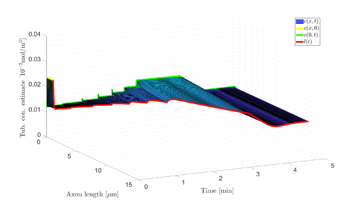
(a)

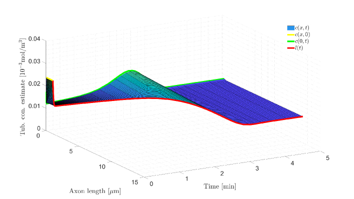
(b)

Figure 2: The closed-loop response of the designed full-state feedback control system for continuous-time and event-triggered control law.

For $M_{j}>0$, we easily demonstrate that $M_{j}<M_{0}$ using Lemma 4, ensuring the norm estimate from Lemma 3 holds. Thus, we set $M_{j}\leq p^{*}$, where $p^{*}$ is a non-zero root of the polynomial for $V>0$.

$$-\alpha^{*}V+\xi_{1}V^{3/2}+\xi_{2}V^{2}+\xi_{3}V^{5/2}+\xi_{4}V^{3}+\xi_{5}V^{7/2}=0$$ (113)

Since $\alpha^{*}$, and $\xi_{i}$ are all positive, at least one positive root exists for the polynomial in (113). Therefore, (106) implies

$$\dot{V}(t)\leq-\frac{\alpha^{*}}{2}V(t)$$ (114)

for $t\in(t_{j},t_{j+1})$, $j\in\mathbb{N}$ where $M_{j}=\min\left\{M_{0},p^{*}\right\}$. The continuity of $V(t)$ in this interval implies $V(t_{j+1}^{-})=V(t)$ and $V(t_{j}^{+})=V(t_{j})$ where $t_{j}^{+}$ and $t_{j}^{-}$ are right and left limits of $t=t_{j}$, respectively. Thus, we have

$$V(t_{j+1})\leq\exp(-\alpha^{*}(t_{j+1}-t_{j}))V(t_{j})$$ (115)

which completes the proof of Lemma 5. ∎

For any $t\geq 0$ in $t\in[t_{j},t_{j+1})$, $j\in\mathbb{N}$, we obtain

$$V(t)\leq e^{-\alpha^{*}(t-t_{j})}V(t_{j})\leq e^{-\alpha^{*}t}V(0)$$ (116)

Recalling $m(t)<0$ and (98), we have

$$d_{1}V_{1}(t)+V_{2}(t)+d_{2}V_{3}(t)\leq e^{-\alpha^{*}t}V(0)$$ (117)

which means that

$$d_{1}\frac{1}{2}||w||^{2}+\frac{1}{2}||w_{x}||^{2}+d_{2}X(t)^{\top}PX(t)$$

$$\leq e^{-\alpha^{*}t}\left(\frac{d_{1}}{2}||w(0)||^{2}+\frac{1}{2}||w_{x}(0)||^{2}+d_{2}X(0)^{\top}PX(0)-m(0)\right)$$

Therefore, we can derive the following norm estimate:

$$||w||^{2}+||w_{x}||^{2}+X(t)^{\top}X(t)$$

$$\leq e^{-\alpha^{*}t}\sqrt{\frac{\frac{d_{1}}{2}||w(0)||^{2}+\frac{1}{2}||w_{x}(0)||^{2}+d_{2}X(0)^{\top}PX(0)-m(0)}{\min\left\{\frac{d_{1}}{2},\frac{1}{2},\frac{d_{2}}{\lambda_{\rm max}(P)}\right\}}}.$$

This confirms the local exponential stability of the system (III-B)-(59) in the $\mathcal{H}_{1}$-norm. By exploiting the backstepping transformation’s invertibility and norm equivalence, we also establish the local exponential stability of the original system (1)-(5) in the $\mathcal{H}_{1}$ norm, concluding the proof of Theorem 2.

VI Numerical Simulations

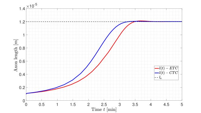
(a)

Figure 3: The closed-loop response of the continuous-time and event-triggered control law for $l_{s}=12\mu m$

TABLE I: Biological constants and control parameters

Parameter	Value	Parameter	Value
$D$	$10\times 10^{-12}m^{2}/s$	$\tilde{r}_{\rm g}$	$0.053$
$a$	$1\times 10^{-8}m/s$	$\gamma$	$10^{4}$
$g$	$5\times 10^{-7}\ s^{-1}$	$l_{\rm c}$	$4\mu m$
$r_{\rm g}$	$1.783\times 10^{-5}\ m^{4}/(mols)$	$l_{s}$	$12\mu m$
$c_{\infty}$	$0.0119\ mol/m^{3}$	$l_{0}$	$1\mu m$

In this section, we conduct a numerical analysis of the plant dynamics (equations (1) to (5) utilizing the control law (defined by (50)) and incorporating the event triggering mechanism (as defined in Definition 1). The model employs biological constants and control parameters from Table 1, with initial conditions set to $c_{0}(x)=2c_{\infty}$ for the tubulin concentration along the axon and $l_{0}=1\mu m$ for the initial axon length. The control gain parameters are chosen as $k_{1}=-0.001$ and $k_{2}=4\times 10^{13}$. The event-triggering mechanism parameters are set as follows: $m(0)=-0.5$, $\beta_{1}=1.634\times 10^{22}$, $\beta_{2}=5.229\times 10^{12}$, $\beta_{3}=6.569\times 10^{-14}$, $\beta_{4}=2.614\times 10^{13}$, $\beta_{5}=2.94\times 10^{-12}$, $\rho=4\times 10^{22}$, $\eta=100$ and $\sigma=0.5$. In Fig. LABEL:fig:1a and LABEL:fig:1b, we present the evolution of tubulin concentration along the axon for both continuous-time control law and event-triggered control.

Fig. 2 shows axon growth convergence under continuous-time and event-triggered control laws. Both methods achieve the desired $12\mu m$ length from an initial $1\mu m$ in about 3.5 minutes. In Fig. 3a, we compare ETC control inputs for $\eta=1$ and $\eta=1000$ with $\sigma=0.5$, showing similar convergence rates. Notably, the ETC controller with $\eta=1000$ samples faster. In Fig. 3b, fixing $\eta$ at $100$ and varying $\sigma$ to $0.8$ results in faster and more frequent sampling, leading to quicker convergence compared to $\sigma=0.1$.

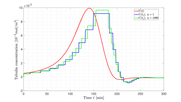
(a)

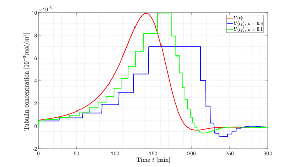
(b)

Figure 4: Comparison of ETC input for different $\eta$ and $\sigma$ design parameters

VII Conclusion

This paper explores a dynamic event-triggering boundary control approach for axonal growth modeling. It addresses the avoidance of Zeno behavior and offers a local stability analysis of the closed-loop system. Future research will focus on investigating periodic event-triggering and self-triggering boundary control methods, which are more suitable for digital implementations.

References

- [1] K.-E. Åarzén, “A simple event-based pid controller,” IFAC Proceedings Volumes, vol. 32, no. 2, pp. 8687–8692, 1999.
- [2] E. J. Bradbury and L. M. Carter, “Manipulating the glial scar: chondroitinase abc as a therapy for spinal cord injury,” Brain research bulletin, vol. 84, no. 4-5, pp. 306–316, 2011.
- [3] J.-M. Coron, R. Vazquez, M. Krstic, and G. Bastin, “Local exponential h^2 stabilization of a 2times2 quasilinear hyperbolic system using backstepping,” SIAM Journal on Control and Optimization, vol. 51, no. 3, pp. 2005–2035, 2013.
- [4] C. Demir, S. Koga, and M. Krstic, “Neuron growth control by pde backstepping: Axon length regulation by tubulin flux actuation in soma,” in 2021 60th IEEE Conference on Decision and Control (CDC), 2021, pp. 649–654.
- [5] ——, “Input delay compensation for neuron growth by pde backstepping,” IFAC-PapersOnLine, vol. 55, no. 36, pp. 49–54, 2022.
- [6] ——, “Neuron growth output-feedback control by pde backstepping,” in 2022 American Control Conference (ACC). IEEE, 2022, pp. 4159–4164.
- [7] S. Diehl, E. Henningsson, A. Heyden, and S. Perna, “A one-dimensional moving-boundary model for tubulin-driven axonal growth,” Journal of theoretical biology, vol. 358, pp. 194–207, 2014.
- [8] S. Ecklebe, F. Woittennek, C. Frank-Rotsch, N. Dropka, and J. Winkler, “Toward model-based control of the vertical gradient freeze crystal growth process,” IEEE Transactions on Control Systems Technology, 2021.
- [9] N. Espitia, A. Girard, N. Marchand, and C. Prieur, “Event-based control of linear hyperbolic systems of conservation laws,” Automatica, vol. 70, pp. 275–287, 2016.
- [10] N. Espitia, I. Karafyllis, and M. Krstic, “Event-triggered boundary control of constant-parameter reaction–diffusion pdes: A small-gain approach,” Automatica, vol. 128, p. 109562, 2021.
- [11] N. Espitia, A. Girard, N. Marchand, and C. Prieur, “Event-based boundary control of a linear hyperbolic system via backstepping approach,” IEEE Transactions on Automatic Control, vol. 63, no. 8, pp. 2686–2693, 2018.
- [12] A. Girard, “Dynamic triggering mechanisms for event-triggered control,” IEEE Transactions on Automatic Control, vol. 60, no. 7, pp. 1992–1997, 2014.
- [13] W. P. Heemels, K. H. Johansson, and P. Tabuada, “An introduction to event-triggered and self-triggered control,” in 2012 ieee 51st ieee conference on decision and control (cdc). IEEE, 2012, pp. 3270–3285.
- [14] W. Heemels, J. Sandee, and P. Van Den Bosch, “Analysis of event-driven controllers for linear systems,” International journal of control, vol. 81, no. 4, pp. 571–590, 2008.
- [15] M. Izadi, J. Abdollahi, and S. S. Dubljevic, “Pde backstepping control of one-dimensional heat equation with time-varying domain,” Automatica, vol. 54, pp. 41–48, 2015.
- [16] E. M. Izhikevich, Dynamical systems in neuroscience. MIT press, 2007.
- [17] E. R. Kandel, J. H. Schwartz, T. M. Jessell, S. Siegelbaum, A. J. Hudspeth, and S. Mack, Principles of neural science. McGraw-hill New York, 2000, vol. 4.
- [18] S. Karimi-Abdolrezaee, E. Eftekharpour, J. Wang, D. Schut, and M. G. Fehlings, “Synergistic effects of transplanted adult neural stem/progenitor cells, chondroitinase, and growth factors promote functional repair and plasticity of the chronically injured spinal cord,” Journal of Neuroscience, vol. 30, no. 5, pp. 1657–1676, 2010.
- [19] C. Koch, Biophysics of computation: information processing in single neurons. Oxford university press, 2004.
- [20] E. Kofman and J. H. Braslavsky, “Level crossing sampling in feedback stabilization under data-rate constraints,” in Proceedings of the 45th IEEE Conference on Decision and Control. IEEE, 2006, pp. 4423–4428.
- [21] S. Koga, C. Demir, and M. Krstic, “Event-triggered safe stabilizing boundary control for the stefan pde system with actuator dynamics,” in 2023 American Control Conference (ACC). IEEE, 2023, pp. 1794–1799.
- [22] S. Koga and M. Krstic, Materials Phase Change PDE Control and Estimation: From Additive Manufacturing to Polar Ice. Springer Nature, 2020.
- [23] M. Krstic, “Compensating actuator and sensor dynamics governed by diffusion PDEs,” Systems & Control Letters, vol. 58, no. 5, pp. 372–377, 2009.
- [24] M. Krstic and A. Smyshlyaev, Boundary control of PDEs: A course on backstepping designs. SIAM, 2008.
- [25] H. Lee, R. J. McKeon, and R. V. Bellamkonda, “Sustained delivery of thermostabilized chabc enhances axonal sprouting and functional recovery after spinal cord injury,” Proceedings of the National Academy of Sciences, vol. 107, no. 8, pp. 3340–3345, 2010.
- [26] X. Z. Liu, X. M. Xu, R. Hu, C. Du, S. X. Zhang, J. W. McDonald, H. X. Dong, Y. J. Wu, G. S. Fan, M. F. Jacquin et al., “Neuronal and glial apoptosis after traumatic spinal cord injury,” Journal of Neuroscience, vol. 17, no. 14, pp. 5395–5406, 1997.
- [27] R. B. Maccioni, J. P. Muñoz, and L. Barbeito, “The molecular bases of alzheimer’s disease and other neurodegenerative disorders,” Archives of medical research, vol. 32, no. 5, pp. 367–381, 2001.
- [28] D. R. McLean, A. van Ooyen, and B. P. Graham, “Continuum model for tubulin-driven neurite elongation,” Neurocomp., vol. 58, pp. 511–516, 2004.
- [29] H. Oliveri and A. Goriely, “Mathematical models of neuronal growth,” Biomechanics and Modeling in Mechanobiology, vol. 21, no. 1, pp. 89–118, 2022.
- [30] B. Petrus, J. Bentsman, and B. G. Thomas, “Enthalpy-based feedback control algorithms for the stefan problem,” in 2012 IEEE 51st IEEE Conference on Decision and Control (CDC), 2012, pp. 7037–7042.
- [31] R. Postoyan, A. Anta, D. Nešić, and P. Tabuada, “A unifying lyapunov-based framework for the event-triggered control of nonlinear systems,” in 2011 50th IEEE conference on decision and control and European control conference. IEEE, 2011, pp. 2559–2564.
- [32] B. Rathnayake and M. Diagne, “Event-based boundary control of one-phase stefan problem: A static triggering approach,” in 2022 American Control Conference (ACC). IEEE, 2022, pp. 2403–2408.
- [33] ——, “Event-based boundary control of the stefan problem: A dynamic triggering approach,” in 2022 IEEE 61st Conference on Decision and Control (CDC). IEEE, 2022, pp. 415–420.
- [34] G. A. Susto and M. Krstic, “Control of pde–ode cascades with neumann interconnections,” Journal of the Franklin Institute, vol. 347, no. 1, pp. 284–314, 2010.
- [35] S. Tang and C. Xie, “State and output feedback boundary control for a coupled pde–ode system,” Syst. Contr. Lett., vol. 60, no. 8, pp. 540–545, 2011.
- [36] M. P. Van Veen and J. Van Pelt, “Neuritic growth rate described by modeling microtubule dynamics,” Bulletin of mathematical biology, vol. 56, no. 2, pp. 249–273, 1994.
- [37] H. Yu, M. Diagne, L. Zhang, and M. Krstic, “Bilateral boundary control of moving shockwave in lwr model of congested traffic,” IEEE Transactions on Automatic Control, 2020.