Construction of a circuit for the simulation of a Hamiltonian with a tridiagonal matrix representation

Abstract

The simulation of quantum systems is an area where quantum computers are promised to achieve an exponential speedup over classical simulations. State-of-the-art quantum algorithms for Hamiltonian simulation achieve this by reducing the amount of oracle queries. Unfortunately, these predicted speedups may be limited by a sub-optimal oracle implementation, thus limiting their use in practical applications. In this paper we present a construction of a circuit for simulation of Hamiltonians with a tridiagonal matrix representation. We claim efficiency by estimating the resulting gate complexity. This is done by determining all Pauli strings present in the decomposition of an arbitrary tridiagonal matrix and dividing them into commuting sets. The union of these sets has a cardinality exponentially smaller than that of the set of all Pauli strings. Furthermore, the number of commuting sets grows logarithmically with the size of the matrix. Additionally, our method for computing the decomposition coefficients requires exponentially fewer multiplications compared to the direct approach. Finally, we exemplify our method in the case of the Hamiltonian of the one-dimensional wave equation and numerically show the dependency of the number of gates on the number of qubits.

1 Introduction

Simulation of quantum Hamiltonians is one of the first directions that emerged in the field of quantum computing, since it is believed that quantum simulation should be faster on a quantum device than on a classical one [1]. Over the years this field has evolved and great progress has been made since the first description by Lloyd [2] in $1996$, where a Hamiltonian for local interactions was considered. Latest developed techniques, such as quantum walk algorithm [3], simulation by Qubitization [4], and others [5, 6, 7, 8] are often described in terms of calls to an oracle, but the construction of the oracle itself is usually not considered in detail. It is worth noting that without an efficient circuit, the number of gates in the algorithm may be very large and a theoretical exponential speedup may not lead to a useful algorithm for practical applications.

One way to implement a circuit for the Hamiltonian simulation on a quantum computer is to decompose the Hamiltonian $H$ into a sum of Pauli strings (tensor product of Pauli matrices) and approximate the operator $e^{-iHt}$ with product formulae [9, 10]. With a naive approach, the number of Pauli strings to consider is $4^{n}$ if the size of $H$ is $2^{n}\times 2^{n}$. It has been shown that modeling $e^{-iHt}$ using this approach is more efficient if one can group resulting Pauli strings into commuting sets [11, 12, 13].

In general, finding the maximal set of commuting sets by brute force requires exponential time. The problem of partitioning a Hamiltonian decomposition in the Pauli basis featuring sets of commuting operators was studied in the framework of simultaneous measurements [14, 15]. Typically, this problem may be solved by building a graph with Pauli strings as nodes, connected if they commute. The graph coloring algorithm to find commuting fragments (cliques) is NP-Complete, but good heuristics exist [16].

In this work we consider Hamiltonians of a special kind represented by tridiagonal matrices. Tridiagonal matrices come to light in many different areas of mathematical and applied sciences, commonly in the discretization of differential equations [17, 18] where they represent discretized version of differential operators.

The proposed procedure provides a partitioning of the Pauli string decomposition of the tridiagonal matrices into sets of internally commuting Pauli strings and the coefficients (weights) for each Pauli string in the decomposition. It automatically leverages the structure of the tridiagonal matrix to remove the majority of the redundant Pauli strings with zero coefficients and provides an upper bound for the number of Pauli strings with non-zero weights. Moreover, it contains a formula for calculation of the weights (basis coefficients) separate from the symbolic generation of Pauli strings.

This work is organized as follows. In Section 2 we introduce the notation and useful mathematical constructs. The decomposition algorithm for an arbitrary tridiagonal matrix is described in Section 3, followed by specific variants for real and real symmetric tridiagonal matrices. Section 4 is devoted to the special case of a symmetrized matrix $H$ constructed from a real matrix $B$ such that both $B$ and $B^{T}$ are off-diagonal. In Section 5 we focus on Hamiltonian simulation, while in Section 6 we illustrate our method with an example of the one-dimensional wave equation. We defer longer proofs of the statements to the Appendix A.

2 Notation and definitions

The Pauli matrices and the identity constitute a basis for the complex vector space of $2\times 2$ matrices and comprises of operators $\mathcal{P}=\{I,X,Y,Z\}$, where

$$\begin{gathered}I=\begin{pmatrix}1&0\\ 0&1\end{pmatrix},X=\begin{pmatrix}0&1\\ 1&0\end{pmatrix},\;\ Y=\begin{pmatrix}0&-i\\ i&0\end{pmatrix},\;\;Z=\begin{pmatrix}1&0\\ 0&-1\end{pmatrix}\end{gathered}$$

A tensor product of several Pauli matrices is called a Pauli string. The length of a Pauli string is the number of Pauli operators in the string and it is exactly $n$ when decomposing a $2^{n}\times 2^{n}$ matrix. Pauli strings act in the $n$-qubit Hilbert space $\mathcal{H}$ of size $2^{n}$. We denote the set of Pauli strings of length $n$ as $\mathcal{P}_{n}$.

The Pauli basis decomposition of an arbitrary matrix $B$ is given by

$$B=\frac{1}{2^{n}}\sum_{j=1}^{M}\alpha_{j}P_{j}\;,\;\;P_{j}\in\mathcal{P}_{n},$$ (1)

where $M$ is the number of terms in the decomposition and $\alpha_{j}\in\mathbb{C}$ in general. Hereinafter we omit tensor multiplication sign when writing Pauli strings (e. g. $X\otimes Y\otimes Z\otimes Y$ is abbreviated as $XYZY$).

Efficient manipulation of Pauli strings is possible with bit arithmetic. For a single bit $x\in\mathbb{B}$ we use the following notation for powers $p\in\mathbb{B}$

$$x^{p}=x\oplus\overline{p}=x\oplus p\oplus 1,$$

where $\oplus$ is the XOR operation, which works as addition modulo 2. Definitions for strings of bits $\mathbf{x}\equiv(x_{1},\dots,x_{n})\in\mathbb{B}^{n}$ where $x_{j}\in\mathbb{B},j=1,\dots,n$ are summarized in Table 1.

Notation	Definition
$\overline{\mathbf{x}}$	Negation, $\overline{\mathbf{x}}=(\overline{x}_{1},\dots,\overline{x}_{n})$
$\mathbf{x}^{\mathbf{y}}$	Exponentiation, $\mathbf{x}^{\mathbf{y}}=(x_{1}^{y_{1}},\dots,x_{n}^{y_{n}})$
$\mathbf{x}\cdot\mathbf{y}$	Inner Product, $\mathbf{x}\cdot\mathbf{y}=\sum_{l=1}^{n}x_{l}y_{l}$
$\delta(\mathbf{x},\mathbf{y})$	Kronecker delta, $\delta(\mathbf{x},\mathbf{y})=\prod_{j=1}^{n}\delta_{x_{j},y_{j}}$
$X^{\mathbf{y}}$	$X^{\mathbf{y}}=\bigotimes_{l=1}^{n}X^{y_{l}}=X^{y_{1}}\otimes\cdots\otimes X^{y_{n}}$
$Z^{\mathbf{y}}$	$Z^{\mathbf{y}}=\bigotimes_{l=1}^{n}Z^{y_{l}}=Z^{y_{1}}\otimes\cdots\otimes Z^{y_{n}}$

Table 1: Notations and their definitions used in this work for operations with bit strings. Here $\mathbf{x}=(x_{1},\dots,x_{n})\in\mathbb{B}^{n}$, $\mathbf{y}=(y_{1},\dots,y_{n})\in\mathbb{B}^{n}$, $X$ and $Z$ are Pauli matrices.

For $\mathbf{x}\in\mathbb{B}^{n}$ we define the vector $\ket{\mathbf{x}}\in(\mathbb{C}^{2})^{\otimes n}$ as

$$\ket{\mathbf{x}}=\bigotimes_{l=1}^{n}\ket{x_{l}}=\ket{x_{1},\dots x_{n}}.$$ (2)

Further we define the function that converts non-negative integers to binary

$$\textrm{BIN}:\mathbb{N}\cup\{0\}\rightarrow\mathbb{B}^{n}.$$ (3)

Note that BIN, as well as the bit string $\mathbf{x}$ are encodings of an integer, where the leftmost bit encodes the lower register. For example, the string $1101$ is the encoding of $1\cdot 1+1\cdot 2+0\cdot 4+1\cdot 8=11$.

To express Pauli strings with $X$ and $Z$ matrices we use bit strings $\mathbf{z},\mathbf{x},\mathbf{p}\in\mathbb{B}^{n}$ and definitions in table 1:

$$Z^{\mathbf{z}}\ket{\mathbf{p}} =\bigotimes_{l=1}^{n}Z^{z_{l}}\ket{p_{l}}=(-1)^{\mathbf{z}\cdot\mathbf{p}}\ket{\mathbf{p}},$$ (4)

$$X^{\mathbf{x}}\ket{\mathbf{p}} =\bigotimes_{l=1}^{n}X^{x_{l}}\ket{p_{l}}=\ket{\overline{\mathbf{p}}^{\mathbf{x}}}.$$ (5)

An arbitrary Pauli string can be defined as the image of the extended Pauli string operator (Walsh function)
$\hat{W}:\mathbb{B}^{n}\times\mathbb{B}^{n}\rightarrow\mathcal{P}_{n}$ as follows

$$\hat{W}(\mathbf{x},\mathbf{z})=i^{\mathbf{x}\cdot\mathbf{z}}X^{\mathbf{x}}Z^{\mathbf{z}}=\bigotimes_{j=1}^{n}i^{x_{j}z_{j}}X^{x_{j}}Z^{z_{j}},$$ (6)

with an ordinary matrix product between $X^{\mathbf{x}}$ and $Z^{\mathbf{z}}$. It can be seen that the Walsh function is bijective. Thus, each Pauli string can be encoded with a unique pair $(\mathbf{x},\mathbf{z})$ and (1) can be rewritten as

$$B=\frac{1}{2^{n}}\sum_{\mathbf{x},\mathbf{z}\in\mathbb{B}^{n}}\beta_{\mathbf{x},\mathbf{z}}\hat{W}(\mathbf{x},\mathbf{z}),$$ (7)

where $\beta_{\mathbf{x},\mathbf{z}}\in\mathbb{C}$. There is one-to-one correspondence between $\alpha_{j}$ from (1) and $\beta_{\mathbf{x},\mathbf{z}}$ in (7).

By $\{P_{1},\;P_{2}\}^{\otimes{n}}$ we denote the $n$-th Cartesian product of the set $\{P_{1},\;P_{2}\}$ with elements interpreted as Pauli strings.

3 Tridiagonal matrix decompositions

We consider an arbitrary band matrix $B\in\mathbb{C}^{N\times N}$, where $N=2^{n}$ of the following form:

$$B=\begin{pmatrix}c_{1}&a_{1}&0&\dots&0&0&0\\ b_{1}&c_{2}&a_{2}&\dots&0&0&0\\ 0&b_{2}&c_{3}&\dots&0&0&0\\ \dots&\dots&\dots&\dots&\dots&\dots&\dots\\ 0&0&0&\dots&c_{N-2}&a_{N-2}&0\\ 0&0&0&\dots&b_{N-2}&c_{N-1}&a_{N-1}\\ 0&0&0&\dots&0&b_{N-1}&c_{N}&\\ \end{pmatrix}$$ (8)

Below we formulate several theoretical results. Theorem 1 provides the maximal possible set of Pauli strings with non-zero coefficients in the decomposition of an arbitrary tridiagonal matrix with complex entries. Then we limit our consideration to tridiagonal matrices with only real entries (Theorem 2) and further we consider only tridiagonal symmetric real matrices ($a_{i}=b_{i}$) in corollary 2 and provide the maximal possible set of Pauli strings with non-zero coefficients in each case, as well as provide a possible partitioning of these strings into sets of internally commuting operators.

3.1 Pauli strings present in the decomposition

We formulate the following theorem regarding the decomposition of an arbitrary tridiagonal matrix $B$ with complex entries shown in (8) into Pauli strings:

Theorem 1 (Decomposition of an arbitrary Tridiagonal matrix).

An arbitrary tridiagonal matrix $B\in\mathbb{C}^{N\times N}$, where $N=2^{n}$, can have Pauli strings in its decomposition with non-zero coefficients only from the union of the following disjoint sets with total cardinality of $(n+1)2^{n}:$
0. $\{I,Z\}$ $\otimes$ $\{I,Z\}$ $\otimes$ $\dots$ $\otimes$ $\{I,Z\}$ $\otimes$ $\{I,Z\}$ $\otimes$ $\{I,Z\}$ 1. $\{I,Z\}$ $\otimes$ $\{I,Z\}$ $\otimes$ $\dots$ $\otimes$ $\{I,Z\}$ $\otimes$ $\{I,Z\}$ $\otimes$ $\{X,Y\}$ 2. $\{I,Z\}$ $\otimes$ $\{I,Z\}$ $\otimes$ $\dots$ $\otimes$ $\{I,Z\}$ $\otimes$ $\{X,Y\}$ $\otimes$ $\{X,Y\}$ 3. $\{I,Z\}$ $\otimes$ $\{I,Z\}$ $\otimes$ $\dots$ $\otimes$ $\{X,Y\}$ $\otimes$ $\{X,Y\}$ $\otimes$ $\{X,Y\}$ $\dots$ n-1. $\{I,Z\}$ $\otimes$ $\{X,Y\}$ $\otimes$ $\dots$ $\otimes$ $\{X,Y\}$ $\otimes$ $\{X,Y\}$ $\otimes$ $\{X,Y\}$ n. $\{X,Y\}$ $\otimes$ $\{X,Y\}$ $\otimes$ $\dots$ $\otimes$ $\{X,Y\}$ $\otimes$ $\{X,Y\}$ $\otimes$ $\{X,Y\}$ $\scriptstyle n$

The first step in the procedure for decomposition of a tridiagonal matrix in the Pauli basis (1) consists of symbolic generation of Pauli strings starting from all diagonal $\{I,Z\}$ operators to all anti-diagonal operators $\{X,Y\}$ by replacing one diagonal operator on the right with an anti-diagonal operator at each step $m$. The decomposition weights can be calculated later, based on the selected Pauli strings, see 3.2. Note that the cardinality of the union in Theorem 1 is based on the structure of an arbitrary tridiagonal matrix, weightcalculation may result in a fewer number of Pauli strings in the decomposition.

We denote the sets in Theorem 1 as

$$S_{m,\pm}^{n}=\{I,\;Z\}^{\otimes({n-m})}\otimes\{X,Y\}^{\otimes m},\quad m=0,\dots,n.$$ (9)

When $m=n$ ($m=0$) the first (second) tensor product is omitted. Each step $m$ generates $2^{n}$ Pauli strings, we divide these strings in two sets named $S_{m,+}$ and $S_{m,-}$, where $+$ indicates that the number of $Y$ operators in every Pauli string in the set is even and $-$ indicates that this number is odd. When $m=0$, there are no $Y$ operators, so we will denote it as $S_{0}$. Note that each $m$ corresponds to a row labeled by $m$ in Theorem 1.

The bit string notation from Section 2 provides a concise description of sets $S_{m,\pm}^{n}$ where the correspondence to $m$ is given by bit string $\mathbf{x}$ as follows:

$$\begin{split}S_{m,+}^{n}=\{\hat{W}(\mathbf{x},\mathbf{z}):\mathbf{x}\cdot\mathbf{z}=0(\mathrm{mod}\leavevmode\nobreak\ 2),\leavevmode\nobreak\ \mathbf{x}=V_{m}^{n},\leavevmode\nobreak\ \mathbf{z}\in\mathbb{B}^{n}\},\\ S_{m,-}^{n}=\{\hat{W}(\mathbf{x},\mathbf{z}):\mathbf{x}\cdot\mathbf{z}=1(\mathrm{mod}\leavevmode\nobreak\ 2),\leavevmode\nobreak\ \mathbf{x}=V_{m}^{n},\leavevmode\nobreak\ \mathbf{z}\in\mathbb{B}^{n}\},\end{split}$$ (10)

here $V_{m}^{n}$ is a selector with m bits set to one and the following $n-m$ bits set to zero, like: $v_{j}=(1,...,1,0_{j},...,0)$, formally:

$$V_{m}^{n}=(v_{1}^{m},\dots,v_{n}^{m}),\quad v_{j}^{k}=\begin{cases}1,\;k\geq j\\ 0,\;k<j\end{cases}$$ (11)

Thus, the bit string $\mathbf{x}$ corresponds to $m$ such that the first $m$ positions of the bit string set to one, and the remaining ($n-m$) positions are all zeros. To generate each subset $S_{m,\pm}^{n}$, $\mathbf{z}$ traverses all numbers $0,\dots,n$ and the generated Pauli strings are sorted according to the outcome of $\mathbf{x}\cdot\mathbf{z}$.

Each of the subsets $S_{m,\pm}^{n}$ contains commuting Pauli strings due to the following Lemma:

Lemma 1 (Commutativity criterion).

Let $P=\hat{W}(\mathbf{x},\mathbf{z})$ and $Q=\hat{W}(\mathbf{a},\mathbf{b})$ be two Pauli strings of length $n$, where $\mathbf{x},\mathbf{z},\mathbf{a},\mathbf{b}\in\mathbb{B}^{n}$. Then $P$ and $Q$ commute iff

$$\mathbf{x}\cdot\mathbf{b}=\mathbf{a}\cdot\mathbf{z}\ (\mathrm{mod}\ 2).$$ (12)

Corollary 1.

Let $P=\hat{W}(\mathbf{x},\mathbf{z})$ and $Q=\hat{W}(\mathbf{x},\mathbf{b})$ be two Pauli strings of length $n$, where $\mathbf{x},\mathbf{z},\mathbf{b}\in\mathbb{B}^{n}$. Let the parity of $Y$ operators in both strings be equal, then $P$ and $Q$ commute.

This Lemma and Corollary are proven in Appendix Section A.2. We reach a conclusion that $S_{m,+}^{n}$ and $S_{m,-}^{n}$ each are internally commuting subsets. Therefore, the general matrix decomposition will have $2n+1$ internally commuting subsets.

Analogous to the general case, for a real tridiagonal matrix $B$ the following theorem will hold:

Theorem 2 (Real tridiagonal matrix).

A real tridiagonal matrix $B\in\mathbb{R}^{N\times N}$, where $N=2^{n}$, can have Pauli strings in its decomposition with non-zero coefficients only from the union of $2n+1$ disjoint internally commuting sets $S_{m,\pm}$, $2n$ of which have a cardinality of $2^{n-1}$ each and one of which is given by $S_{0,\pm}$ and has cardinality of $2^{n}.$ The cardinality of the union is $(n+1)2^{n}.$

An important use case is a real symmetric tridiagonal matrix $B$. The symmetry will enable additional cancelations in the decomposition, such that only $S_{m,+}$ may be present. This is reflected in the following Corollary:

Corollary 2 (Real symmetric tridiagonal matrix).

A real symmetric tridiagonal matrix $B\in\mathbb{R}^{N\times N}$, where $N=2^{n}$, can have Pauli strings in its decomposition with non-zero coefficients only from the union of $n+1$ disjoint internally commuting sets, $n$ of which are given by $S_{m,+}$ and have a cardinality of $2^{n-1}$ each and one of which is given by $S_{0}$ and has a cardinality of $2^{n}.$ The cardinality of the union is $(n+2)2^{n-1}.$

For convenience we omit the superscript $n$ in $S_{m,+}^{n}$ and omit the $+$, when the length $n$ and parity is clear from the context.

3.2 Decomposition weights

In order to calculate the coefficients(weights) of our decomposition we observe that it is easier to separate the calculation of the weights for the ”diagonal” and ”off-diagonal” subsets. The matrix $B$ can be written as a sum of the diagonal $D$ and off-diagonal $F$ matrices: $B=D+F$. The diagonal matrix $D$ after decomposition consists of Pauli strings of length $n$ in the subset $S_{0}$ containing only $Z$ and $I$ operators. The coefficients $\beta_{\mathbf{x},\mathbf{z}}$ of corresponding $\hat{W}(\mathbf{x},\mathbf{z})$ within this first internally commuting set can be calculated as

$$\beta_{\mathbf{0},\mathbf{z}}=\sum_{p=0}^{2^{n}-1}(-1)^{\mathbf{z}\cdot{\textrm{BIN}(p)}}c_{p},$$ (13)

where $c_{p}$ is a diagonal element of the matrix $B$ as in (8) and $\mathbf{0}$ is $(0,\dots,0)$, $\mathbf{z}\in\mathbb{B}^{n}$.

For the off-diagonal matrix $F$, the weights $\beta_{\mathbf{x},\mathbf{z}}$ of the decomposition (see (7)) may be calculated for each $\hat{W}(\mathbf{x},\mathbf{z})$ in a subset $S_{m,\pm}$ given in (9) as follows:

$$\begin{split}\beta_{\mathbf{x},\mathbf{z}}=\sum_{p=0}^{2^{n}-2}i^{\mathbf{x}\cdot\mathbf{z}}(-1)^{\mathbf{z}\cdot{\textrm{BIN}(p)}}\cdot\delta({\textrm{BIN}(p+1)},\overline{{\textrm{BIN}(p)}}^{\mathbf{x}})\cdot a_{p}\\ +\sum_{p=1}^{2^{n}-1}i^{\mathbf{x}\cdot\mathbf{z}}(-1)^{\mathbf{z}\cdot{\textrm{BIN}(p)}}\cdot\delta({\textrm{BIN}(p-1)},\overline{{\textrm{BIN}(p)}}^{\mathbf{x}})\cdot b_{p-1}\end{split}$$ (14)

where $(\mathbf{x},\mathbf{z})$ corresponds to (10), $a_{p}$ and $b_{p}$ are the off-diagonal elements of matrix $B$ as in (8). The expression $\overline{{\textrm{BIN}(p)}}^{\mathbf{x}}$ is calculated as the bit-wise xor of bit string $\mathbf{x}$ with the inverted bit string $\mathbf{p}$.

Note that (14) holds only for the decomposition of off-diagonal elements, while (13) only for the diagonal elements of matrix $B$. These formulae are derived in Appendix A.1.

3.3 Visualization of commuting subsets

To establish some intuition for such decomposition we show which elements of $B$ are targeted by each subset $S_{m}$. It was already mentioned that the diagonal consists of Pauli strings containing only $Z$ and $I$ operators, thus it corresponds to $S_{0}$. For the off-diagonal elements we are left with $n$ subsets $S_{m,\pm}$ specified in (9). To show the correspondence, we consider the off-diagonal component $F$ of a real symmetric matrix $B$ for $n=4$. For a symmetric matrix (see Corollary 2) we have the following subsets with size $2^{n-1}=2^{3}$:

$$S_{1,+}=\{ I,Z\}^{\otimes 3}\otimes\{X\},$$

$$S_{2,+}=\{ I,Z\}^{\otimes 2}\otimes\{XX,YY\},$$

$$S_{3,+}=\{ I,Z\}\otimes\{XXX,XYY,YXY,YYX\},$$

$$S_{4,+}=\{ XXXX,XXYY,XYXY,XYYX,$$

$$YXYX,YXXY,YYXX,YYYY\}.$$

Figure 1 shows how these subsets correspond to the elements of a $2^{4}\times 2^{4}$ matrix $B$. Each $S_{m,+},\;m=1,\dots,4$ is given a color and the structure is apparent. The length of the anti-diagonal segment is equal to $2^{m}$, where $m$ is the number of the $\{X,Y\}$ Pauli operators on the right in the $S_{m}$ expression.

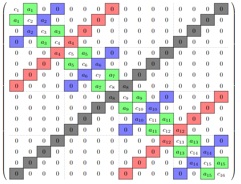
Figure 1: Illustrating correspondence of the sets $S_{m,+}$ to matrix $B$. Colors: $S_{1}$ – green, $S_{2}$ – blue, $S_{3}$ – red, $S_{4}$ – black.

The said structure appears not only for real symmetric matrices. It follows from the associativity of the tensor product where we take the $n-m$ matrices from the set $\{I,Z\}$ on the left with $m$ matrices from the set $\{X,Y\}$ on the right. For each Pauli string $P$ from the subset $S_{m,\pm}$ we have:

$$P=P_{D}\otimes P_{A},$$ (15)

where $P_{D}$ is a diagonal matrix of size $2^{n-m}\times 2^{n-m}$ and $P_{A}$ is an anti-diagonal matrix of size $2^{m}\times 2^{m}$.

4 Decomposition for a symmetrized matrix $H$

A Hermitian matrix $H$ can be constructed from any matrix $B$ by anti-symmetrization:

$$H=\begin{pmatrix}0&B\\ B^{\dagger}&0\\ \end{pmatrix}.$$ (16)

As before, we consider the case where the matrix $B$ is tridiagonal of size $2^{n}\times 2^{n}$, therefore the size of $H$ is $2^{n+1}\times 2^{n+1}$. Here we assume $B$ to be real and therefore $H$ is symmetric. The following statement holds:

Corollary 3.

The number of terms in the decomposition of a symmetric matrix $H$ given by (16) is equal to the number of terms in the decomposition of the real matrix $B$ and is bounded above by $(n+1)2^{n}$. The Pauli strings in the decomposition of $H$ can be partitioned into the following subsets of commuting strings:

$$S_{m}=\{\widehat{X,Y}\}\bigotimes_{1}^{n-m}\{I,Z\}\bigotimes_{1}^{m}\{X,Y\},\;\;m=0,\dots,n,$$ (17)

where the expression $\widehat{\{X,Y\}}$ selects $X$ or $Y$ such that the number of $Y$ operators in each Pauli string is even.

The weights of the decomposition of $H$ may be calculated using formulae (13) and (14). For any square matrix $B$ with its Pauli decomposition given in (7) the following equality holds:

$$H=\frac{1}{2^{n}}\sum_{\mathbf{x},\mathbf{z}\in\mathbb{B}^{n}}\left(\Re{\beta_{\mathbf{x},\mathbf{z}}}X-i\Im{\beta_{\mathbf{x},\mathbf{z}}}XZ\right)\otimes\hat{W}(\mathbf{x},\mathbf{z}).$$ (18)

For details see Appendix A.3.

Consider a symmetric matrix $H$ as in (16) consisting of $B$ and $B^{T}$ with $n=4$ as an example. According to Corollary 3, Pauli strings in decomposition of $H$ can be arranged into the following sets:

$S_{0}=$	$X$	$\otimes$	$\{I,Z\}$	$\otimes$	$\{I,Z\}$	$\otimes$	$\{I,Z\}$	$\otimes$	$\{I,Z\}$,
$S_{1}=$	$\widehat{\{X,Y\}}$	$\otimes$	$\{I,Z\}$	$\otimes$	$\{I,Z\}$	$\otimes$	$\{I,Z\}$	$\otimes$	$\{X,Y\}$,
$S_{2}=$	$\widehat{\{X,Y\}}$	$\otimes$	$\{I,Z\}$	$\otimes$	$\{I,Z\}$	$\otimes$	$\{X,Y\}$	$\otimes$	$\{X,Y\}$,
$S_{3}=$	$\widehat{\{X,Y\}}$	$\otimes$	$\{I,Z\}$	$\otimes$	$\{X,Y\}$	$\otimes$	$\{X,Y\}$	$\otimes$	$\{X,Y\}$,
$S_{4}=$	$\widehat{\{X,Y\}}$	$\otimes$	$\{X,Y\}$	$\otimes$	$\{X,Y\}$	$\otimes$	$\{X,Y\}$	$\otimes$	$\{X,Y\}$.

These are similar to subsets which arise in the decomposition of a real symmetric matrix $B$, but now the size of each subset is $2^{n}$. This follows from the fact that the terms with an odd number of $Y$ operators, which were zero for the real symmetric case, now appear in the decomposition because the $Y$ operator can be selected as the leading term to make the number of $Y$ operators even (see Corollary 2). Figure 2 shows which elements correspond to which set for the matrix $H$ of size $2^{5}\times 2^{5}$.

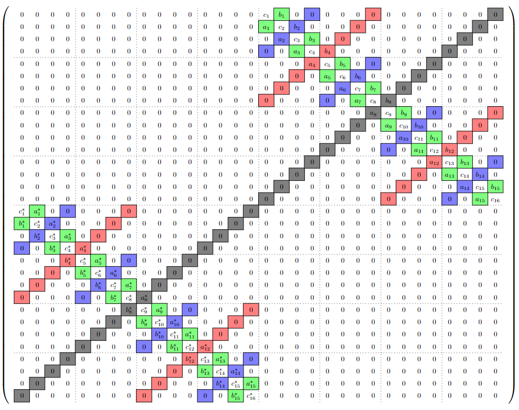
Figure 2: Illustrating correspondence of the sets $S_{m}$ to the matrix $H$ of size $2^{5}\times 2^{5}$ with $B$ and $B^{\dagger}$ of size $2^{4}\times 2^{4}$. Color code: $S_{1}$ – green, $S_{2}$ – blue, $S_{3}$ – red, $S_{4}$ – black. $S_{0}$ corresponds to the diagonal of each B matrix.

5 Circuit for Hamiltonian Simulation

We have shown the two steps in matrix decomposition, namely the generation of Pauli strings based on matrix structure and the calculation of decomposition weights. Importantly, Pauli strings are assembled into commuting sets. The information about commuting sets may serve to reduce the circuit complexity of Hamiltonian simulation [12] and to accelerate simulation of quantum dynamics on a classical computer [11]. In this section we use this approach to construct a circuit for Hamiltonian simulation.

The parameters that should be taken into account when implementing the evolution of the Hamiltonian [4] include the number of system qubits $n$, evolution time $t$, target error $\epsilon$, and how information on the Hamiltonian $H$ is accessed by the quantum computer. Our circuit does not require additional qubits, and it does not use oracles to access information. As we organized a large number of Pauli strings into an exponentially smaller number of commuting subsets we could expect improvement in the accuracy according to the Trotterization formula.

The task of Hamiltonian simulation is to implement the operator $e^{-i\hat{H}t}$ on a quantum device. For an operator $\hat{H}$ represented by a tridiagonal or symmetrized (as discussed in Section 4) matrix $H$ the quantum circuit is constructed as follows.

First we generate internally commuting sets of Pauli strings $\{S_{m,\pm}^{n}\}$ needed for the decomposition of $H$. These strings can be simultaneously diagonalized [11, 12]. As an example, Table 2 contains the diagonalization operators $D_{k}$ for the real symmetrical tridiagonal matrix of size $2^{4}$ discussed in Section 3.3. Note that $D_{0}$ is an identity since the $S_{0}$ set is already diagonal. These operations, i.e. generation of the commuting sets of Pauli strings and optional simultaneous diagonalization, do not need to be repeated when matrix changes values, making this approach suitable for use in variational algorithms [19, 20].

$D_{k}$	Simultaneous diagonalization operators for subset $S_{k}$
$D_{1}$	$HHHI$ $CX(1,4)$ $CX(2,4)$ $CX(3,4)$ $HHHH$
$D_{2}$	$HHHI$ $CX(1,3)$ $CX(1,4)$ $CX(2,3)$ $CX(2,4)$ $CX(3,4)$
	$CZ(1,4)$ $CZ(2,4)$ $CZ(3,4)$ $HHHH$
$D_{3}$	$HHHI$ $CX(1,3)$ $CX(1,4)$ $CX(2,4)$ $CX(3,4)$
	$CZ(1,4)$ $CZ(2,4)$ $CZ(3,4)$ $HHHH$
$D_{4}$	$HHHI$ $CX(1,2)$ $CX(1,4)$ $CX(2,3)$
	$CZ(1,3)$ $CZ(3,4)$ $HHHH$

Table 2: Diagonalization operators $D_{k}$ for a real symmetric tridiagonal matrix of size $2^{4}$ consisting of the Hadamard operators $H$, the Controlled-NOT $CX(c,t)$, and Controlled-Z $CZ(c,t)$ operators, where $c$ and $t$ are the control and the target qubits, respectively. Qubits are labeled from $1$ to $4$.

When a quantum state evolves in time under the action of $e^{-iHt}$ and the matrix $H$ is represented in Pauli basis as in formula (1) (or, equivalently, as in (7)) the Lie-Trotter product formula [9] and its higher order variants [10] should be implemented taking the internally commuting sets into account. Given the time evolution governed by the Hermitian $H$ and the number of Trotter repetitions $r$, using our decomposition we have:

$$e^{-itH} =\exp\left(\frac{-it}{2^{n}}\sum_{\mathbf{x},\mathbf{z}\in\mathbb{B}^{n}}\beta_{\mathbf{x},\mathbf{z}}\hat{W}(\mathbf{x},\mathbf{z})\right)\approx\left[\prod_{k=0}^{2n}\exp\left(\frac{-it}{2^{n}r}\tilde{S}_{k}\right)\right]^{r},$$ (19)

where $\tilde{S}_{k}=\sum_{\mathbf{z}}\beta_{\mathbf{x}_{k},\mathbf{z}}\hat{W}(\mathbf{x}_{k},\mathbf{z})$ are renumbered Pauli strings from subsets $S_{m,\pm}$ defined in (10), which contain up to $2^{n}$ terms each. The approximation is constructed with a Lie-Trotter product formula for $2n+1$ internally commuting sets $S_{m,\pm}$ of Pauli strings. The expression (19) can be diagonalized as

$$\prod_{k=0}^{2n}\exp(\frac{-it}{2^{n}r}\tilde{S}_{k}) =\prod_{k=0}^{2n}\exp\left(\frac{-it}{2^{n}r}\sum_{\mathbf{z}}\beta_{\mathbf{x}_{k},\mathbf{z}}\hat{W}(\mathbf{x}_{k},\mathbf{z})\right)$$

$$=\prod_{k=0}^{2n}D^{\dagger}_{k}\exp\left(\frac{-it}{2^{n}r}\sum_{\mathbf{z}}\beta_{\mathbf{x}_{k},\mathbf{z}}\Lambda_{k,\mathbf{z}}\right)D_{k},$$ (20)

where $D_{k}$ is the diagonalization operator for each subset $\tilde{S}_{k}$. The number $k$ fixes the string $\mathbf{x}_{k}$, and the inner summation over $\mathbf{z}$ covers the commuting subset as in (10). The operator $\Lambda_{k,\mathbf{z}}$ is a diagonal operator corresponding to $\hat{W}(\mathbf{x}_{k},\mathbf{z})$. It is important to note that the coefficients $\beta$ remain the same after diagonalization, or in other words, diagonalization depends only on the structure of the matrix (i.e., depends only on the Pauli subset) and does not depend on the values of the matrix elements. The computation of $D_{k}$ is done by using Clifford algebras [11, 12]. The $D_{k}$ operators consist of the combinations of the single-qubit Hadamard operators and the two-qubit $CX$ and $CZ$ operators and the size of $D_{k}$ scales as $O(n^{2})$, where $n$ is number of qubits.

It can be seen that in order to evaluate the propagator $e^{-iHt}$ as in (19), (5) one has to compute the coefficients $\beta_{\mathbf{x},\mathbf{z}}$ and implement $2n+1$ diagonal exponents $\Lambda_{k,\mathbf{z}}$. The coefficients can be computed by using formulae (13) and (14) and in order to implement $2n+1$ diagonal exponents one can use the results from [21] where it is shown that the gate count for a circuit which implements the diagonal exponent can be reduced to $O(N^{\prime})$ gates with $N^{\prime}<2^{n}$, without ancillary qubits.

Combining all the results together we obtain gate complexity estimated as $O(r(2n+1)(2n^{2}+2^{n}))=O(rn2^{n})$ since for one Trotter step for each of $2n+1$ commuting sets one needs to implement $D$, $D^{\dagger}$ and diagonal exponents. When considering the Trotter formula of an arbitrary order $p$, each Trotter step will contain $O(5^{\lfloor p/2\rfloor})$ times more gates, but the accuracy $\epsilon$ will be achieved in fewer steps $r$. In work [10] the Trotterization error considered by leveraging information about commutation and the following scaling is given $\epsilon=O(\frac{\alpha_{\text{comm}}t^{p+1}}{r^{p}})$ with $\alpha_{\text{comm}}=\sum_{j_{1},\dots,j_{p+1}}^{M}\norm{[H_{j_{p+1}}\cdots[H_{j_{2}},H_{j_{1}}]\cdots]}$ and $H=\sum_{j=1}^{M}H_{j}$, where $H_{j}$ are anti-Hermitian (which is the case since simulation of $e^{tH}$ is considered in [10]). It is an interesting question whether it is possible to obtain some tight upper bound for $\alpha_{\text{comm}}$. For now, we will use scaling provided by authors in [22], i.e. $\epsilon=O\left(\frac{\left(2M5^{\lfloor p/2\rfloor-1}\norm{H}t\right)^{p+1}}{r^{p}}\right)$, where $H=\sum_{j=1}^{M}H_{j}$. Note that in this formula $H$ can be considered as the sum of $2n+1$ matrices formed from commuting sets. Thus $M=2n+1$ and resulting number of gates $g$ is given by

$$g=O\left(tn^{2}2^{n}5^{p}\norm{H}\left(\frac{tn\norm{H}}{\epsilon}\right)^{1/p}\right).$$ (21)

This scaling can be made more accurate by taking into account information about the commuting sets. This can be seen for the case where all Pauli strings commute, making the Trotter error equal to zero. It is possible to find some order of Pauli strings that will reduce the error, but since the number of all possible combinations grows exponentially, this is a difficult task [23].

6 Quantum simulation example: Solving wave equation

Tridiagonal matrices arise very often when discretizing derivatives. For example, the solution of the heat equation given as $u_{t}(x,t)=(\kappa(x)u_{x}(x,t))_{x}$ may be written as [18]

$$u(x,t)=e^{Bt}u(x,0),$$ (22)

where $B$ is real symmetric tridiagonal matrix as in Section 3.

Another example is the wave equation. Let us consider it in more detail. Wave equation with amplitude $u(x,t)$ and speed $c(x)$ defined in the interval $x\in[\alpha,\beta]$ is given by:

$$u_{tt}(x,t)=(c^{2}(x)u_{x}(x,t))_{x},\quad u(x,t)\in\mathbb{R}.$$ (23)

We consider the case of the Dirichlet boundary conditions and set the initial conditions for $u$ and $u_{x}$ as follows:

$$\begin{split}u(\alpha,t)&=u(\beta,t)=0,\quad t\in\mathbb{R_{+}},\\ u(x,0)&=g(x),\quad u_{x}(x,0)=0.\end{split}$$ (24)

Following Costa et al. [24] we reduce (23) to the Schrödinger equation. Thus, consider the Hamiltonian in the following form ($h$ is space discretization step):

$$H=\frac{1}{h}\begin{pmatrix}0&B\\ B^{\dagger}&0\\ \end{pmatrix},$$ (25)

which leads to the Schrödinger equation (we use natural units such that $\hbar=1$) with a two component quantum state $\psi=(\phi_{V},\phi_{E})^{T}$

$$\frac{d}{dt}\begin{pmatrix}\phi_{V}\\ \phi_{E}\end{pmatrix}=\frac{-i}{h}\begin{pmatrix}0&B\\ B^{\dagger}&0\\ \end{pmatrix}\begin{pmatrix}\phi_{V}\\ \phi_{E}\end{pmatrix}.$$

This recovers the original (discretized) wave equation (23) if $-BB^{\dagger}=\mathcal{L}$, where $\mathcal{L}$ is the Laplacian giving an approximation of the second order derivative. To apply the method proposed in this work, we need the matrix $B$ to be square and have the size $2^{n}\times 2^{n}$, so we slightly change the matrix $B$ proposed by Costa et al. [24] by writing the Dirichlet boundary conditions explicitly and we have also incorporated $c(x)$ into this matrix:

$$B_{N\times N}=\begin{pmatrix}0&0&0&0&\dots&0&0&0\\ 0&-c_{2}&\;\;c_{3}&0&\dots&0&0&0\\ 0&0&-c_{3}&\;\;c_{4}&\dots&0&0&0\\ \vdots&\vdots&\vdots&\vdots&\ddots&\vdots&\vdots&\vdots\\ 0&0&0&0&\dots&-c_{N-2}&\;\;c_{N-1}&0\\ 0&0&0&0&\dots&0&-c_{N-1}&c_{N}\\ 0&0&0&0&\dots&0&0&0\\ \end{pmatrix}.$$

The wave speed values $c_{k},\;k=1,\dots,N$ with $N=2^{n}$ result from the discretization of the speed profile $c(x)$. The resulting Hamiltonian $H$ has the form described in Section 4. Based on (18) the coefficients of the decomposition are given by:

$$\beta_{\mathbf{0},\mathbf{z}} =-\sum_{k=1}^{2^{n}-2}(-1)^{\mathbf{z}\cdot{\textrm{BIN}(k)}}\cdot c_{k+1},$$ (26)

$$\beta_{\mathbf{x},\mathbf{z}} =\sum_{k=1}^{2^{n}-2}i^{\mathbf{x}\cdot\mathbf{z}}(-1)^{\mathbf{z}\cdot{\textrm{BIN}(k)}}\cdot\delta({\textrm{BIN}(k+1)},\overline{{\textrm{BIN}(k)}}^{\mathbf{x}})\cdot c_{k+2},$$

where $\mathbf{x}=\mathbf{x}(m,n)=V_{m}^{n}$ as defined in (11).

Theoretical gate complexity within error $\epsilon$ for this case can be estimated. In the work [25] the authors show implementation of the algorithm presented in [24, 3]. The gate complexity for the $1d$ wave equation with constant speed is given by $O\left(5^{p}tn^{2}N\left(\frac{tN}{\epsilon}\right)^{1/p}\right)$. The algorithm uses $2n$ qubits to implement oracles and has a big computational overhead.

The gate complexity of our algorithm for solving the wave equation may be estimated as $O\left(5^{p}tn^{2}N^{2}\left(\frac{tnN}{\epsilon}\right)^{1/p}\right)$ since the $\norm{H}\leq|\frac{2c_{\max}}{h}|=O(N)$.

We implemented our algorithm and the dependency of the number of gates on the number of qubits (specifically, the number of discretization points) is shown in Figure 3. The dashed lines show the approximation of the data with $g=\gamma N^{1.5+1/p}n^{2+1/p}$. This scaling is better than the scaling in formula (21) that we obtained analytically. From the picture it also can be seen that the number of gates necessary for obtaining the given accuracy is less than provided in the work [25]. It should be noted that we used only up to $9$ qubits in our simulations.

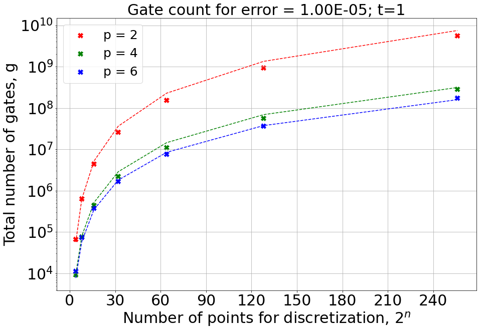
Figure 3: Number of gates needed to obtain an approximation of $e^{-iHt}$ with accuracy $\epsilon=10^{-5}$ for the wave equation with $c(x)=1$. In this plot $t=1$ and the dashed lines depicts scaling as $g=\gamma N^{1.5+1/p}n^{2+1/p}$ with $\gamma=2\leavevmode\nobreak\ 5^{p/2-1}10^{5/p}$ and $n+1$ being the total number of qubits (for $p=6$ where is additional factor $1/2$ in $\gamma$).

7 Conclusion

We have determined all possible Pauli strings that are present in the decomposition of an arbitrary tridiagonal matrix and moreover, have divided them into commuting sets. In particular, we paid attention to symmetric real matrices and symmetrized matrices. In the case of a symmetrized matrix of size $2^{n+1}\times 2^{n+1}$, the resulting Pauli strings can be arranged into $n+1$ commuting sets, each of size $2^{n}$, as shown in Corollary 3 making the total number of strings to be $(n+1)2^{n}$. If these strings were to be obtained by brute force, one would have to sort through all possible options, that is, $4^{n+1}$ strings. We can see that using the presented approach the number of options is exponentially smaller.

We have presented formulas for the decomposition coefficients in Section 3.2. In the case of a symmetrized matrix of size $N\times N$ with $N=2^{n+1}$, the calculation of one coefficient can be estimated to be $O(N\log{N})$ binary multiplications, since in each term we need to compute $O(1)$ products of bit strings with length $O(\log{N})$, see (14). The standard calculation using the trace and matrix multiplication can be estimated as $O(N^{3})$. If we take into account that the matrices are sparse then the complexity of computing one element of the resulting matrix is $O(1)$ making the total complexity $O(N^{2})$. Thus, the presented method of computing the decomposition weights requires exponentially fewer multiplications than the direct approach.

In Section 5, we provided a description of how this approach can be used to construct a circuit for a Hamiltonian simulation and evaluate the resulting gate complexity.

Finally, in Section 6, we considered a problem in which the matrices we have considered arise. We have demonstrated how the Hamiltonian from the wave equation can be decomposed using the method presented in Section 4. We also numerically showed how the number of gates depends on the number of qubits for given accuracy. The number of gates needed to achieve the desired accuracy is fewer than what was used in the implementation of the oracle in [25].

Similar results can be obtained without introducing bit strings and $\hat{W}(\mathbf{x},\mathbf{z})$ operators, but by using Pauli strings directly. Nevertheless, we adopted this way, since using this approach the theorems on commuting sets and the other relevant results can be expressed algebraically in a fairly simple form.

The outcomes of this work raise several questions to which it would be interesting to find answers. For example, one might ask how to obtain sets of commuting rows for matrices with $5$, $7$, or more diagonals? How does division into commuting sets affect Trotter’s error? Is the resulting number of commuting sets minimal? From practical issues, it would be interesting to look at other applications of the resulting partition.

8 Acknowledgements

Competing interests. The authors declare no competing interests. Author contributions. All authors conceived and developed the theory and design of this study and verified the methods. The authors acknowledge the use of Skoltech’s Zhores supercomputer for obtaining the numerical results presented in this paper.

Appendix A Proofs

A.1 Formulae for decomposition coefficients

We call matrix $B$ an upper $l$-diagonal matrix if it has the following structure

$$B=\begin{pmatrix}0&\dots&a_{0}&0&\dots&0\\ \vdots&0&\dots&a_{1}&\vdots&\vdots\\ \vdots&\vdots&\ddots&\vdots&\ddots&\vdots\\ \vdots&\vdots&\vdots&\ddots&\vdots&a_{2^{n}-1-l}\\ \vdots&\vdots&\vdots&\vdots&\ddots&\vdots&\\ 0&\dots&\dots&\dots&\dots&0&\\ \end{pmatrix}$$ (27)

and thus can be written as

$$\begin{split}B=\sum_{k=0}^{2^{n}-1-l}a_{k}\outerproduct{{\textrm{BIN}(k)}}{{\textrm{BIN}(k)}}{{\textrm{BIN}(k+l)}}=\\ \sum_{p,q=0}^{2^{n}-1-l}a_{p}\delta_{{\textrm{BIN}(p+l)},{\textrm{BIN}(q)}}\outerproduct{{\textrm{BIN}(p)}}{{\textrm{BIN}(p)}}{{\textrm{BIN}(q)}}.\end{split}$$ (28)

Similarly, lower $l$-diagonal matrix is introduced as transposed upper $l$-diagonal matrix thus we will not consider this case separately and limit ourselves to upper $l$-diagonal matrix. We also note that Pauli strings present in the decomposition of some matrix $B$ will be the same for $B^{T}$ because all Pauli matrices except $Y$ are symmetric and $Y^{T}=-Y$, so after transposition Pauli strings in decomposition will be the same but coefficients may change a bit.

Lemma 2.

Let $B$ be an upper $l$-diagonal matrix. If a Pauli string $P$ enters the Pauli string decomposition of matrix $B\in\mathbb{C}^{2^{n}\crossproduct 2^{n}}$ non-trivially then $\exists p\in\overline{0,2^{n}-1-l}$:

$${\textrm{BIN}(p+l)}={\textrm{BIN}(p)}\oplus\mathbf{x},$$ (29)

where $\mathbf{x}$ is such that $\hat{W}(\mathbf{x},\mathbf{z})=P$.

Proof.

Let $B\in\mathbb{C}^{2^{n}\crossproduct 2^{n}}$, then decomposition into standard basis may be written as

$$B=\sum_{\mathbf{p},\mathbf{q}\in\mathbb{B}^{n}}b_{\mathbf{p},\mathbf{q}}\outerproduct{\mathbf{p}}{\mathbf{q}}.$$ (30)

On the other hand, decomposition into Pauli basis in $\mathbb{C}^{2^{n}\crossproduct 2^{n}}$ takes form

$$B=\frac{1}{2^{n}}\sum_{\mathbf{x},\mathbf{z}\in\mathbb{B}^{n}}\beta_{\mathbf{x},\mathbf{z}}\hat{W}(\mathbf{x},\mathbf{z}),$$ (31)

where coefficients $\beta_{\mathbf{x},\mathbf{z}}\in\mathbb{C}$. These coefficients can be found by taking the inner product of matrix $B$ and $\hat{W}$ and using formulae (4) and (5) from the main text.

$$\begin{split}&\beta_{\mathbf{x},\mathbf{z}}=\Tr(B\hat{W}(\mathbf{x},\mathbf{z}))=\\ &=\Tr(\sum_{\mathbf{p},\mathbf{q}\in\mathbb{B}^{n}}b_{\mathbf{p},\mathbf{q}}\outerproduct{\mathbf{p}}{\mathbf{q}}i^{\mathbf{x}\cdot\mathbf{z}}X^{\mathbf{x}}Z^{\mathbf{z}})\\ &=\sum_{\mathbf{s}\in\mathbb{B}^{n}}\bra{\mathbf{s}}\left(\sum_{\mathbf{p},\mathbf{q}\in\mathbb{B}^{n}}b_{\mathbf{p},\mathbf{q}}\outerproduct{\mathbf{p}}{\mathbf{q}}i^{\mathbf{x}\cdot\mathbf{z}}X^{\mathbf{x}}Z^{\mathbf{z}}\right)\ket{\mathbf{s}}=\\ &\sum_{\mathbf{s}\in\mathbb{B}^{n}}\sum_{\mathbf{p},\mathbf{q}\in\mathbb{B}^{n}}\bra{\mathbf{s}}b_{\mathbf{p},\mathbf{q}}\outerproduct{\mathbf{p}}{\mathbf{q}}i^{\mathbf{x}\cdot\mathbf{z}}(-1)^{\mathbf{z}\cdot\mathbf{s}}\ket{\mathbf{\overline{s}^{\mathbf{x}}}}=\\ &\sum_{\mathbf{s}\in\mathbb{B}^{n}}\sum_{\mathbf{p},\mathbf{q}\in\mathbb{B}^{n}}b_{\mathbf{p},\mathbf{q}}\innerproduct{\mathbf{s}}{\mathbf{p}}\innerproduct{\mathbf{q}}{\mathbf{\overline{s}^{\mathbf{x}}}}i^{\mathbf{x}\cdot\mathbf{z}}(-1)^{\mathbf{z}\cdot\mathbf{s}}=\\ &\sum_{\mathbf{s}\in\mathbb{B}^{n}}\sum_{\mathbf{p},\mathbf{q}\in\mathbb{B}^{n}}b_{\mathbf{p},\mathbf{q}}\delta_{\mathbf{s},\mathbf{p}}\delta_{\mathbf{q},\mathbf{\overline{s}^{\mathbf{x}}}}i^{\mathbf{x}\cdot\mathbf{z}}(-1)^{\mathbf{z}\cdot\mathbf{s}}=\\ &\sum_{\mathbf{p},\mathbf{q}\in\mathbb{B}^{n}}b_{\mathbf{p},\mathbf{q}}\delta_{\mathbf{q},\overline{\mathbf{p}}^{\mathbf{x}}}i^{\mathbf{x}\cdot\mathbf{z}}(-1)^{\mathbf{z}\cdot\mathbf{p}}=\sum_{\mathbf{p}\in\mathbb{B}}i^{\mathbf{x}\cdot\mathbf{z}}(-1)^{\mathbf{z}\cdot\mathbf{p}}b_{\mathbf{p},\overline{\mathbf{p}}^{\mathbf{x}}}.\end{split}$$ (32)

Since from (28) we have

$$B=\sum_{p,q=0}^{2^{n}-1-l}a_{p}\delta_{{\textrm{BIN}(p+l)},{\textrm{BIN}(q)}}\outerproduct{{\textrm{BIN}(p)}}{{\textrm{BIN}(p)}}{{\textrm{BIN}(q)}},$$ (33)

we can obtain $b_{\mathbf{p},\mathbf{q}}$ by equating the coefficients for $\outerproduct{\mathbf{p}}{\mathbf{q}}$ and $\outerproduct{{\textrm{BIN}(p)}}{{\textrm{BIN}(p)}}{{\textrm{BIN}(q)}}$:

$$b_{\mathbf{p},\mathbf{q}}=b_{{\textrm{BIN}(p)},{\textrm{BIN}(q)}}=a_{p}\delta_{{\textrm{BIN}(p+l)},{\textrm{BIN}(q)}}.$$ (34)

Substituting this expression into (32), we obtain final formula for the coefficients

$$\begin{split}\beta_{\mathbf{x},\mathbf{z}}=\sum_{p=0}^{2^{n}-1-l}i^{\mathbf{x}\cdot\mathbf{z}}(-1)^{\mathbf{z}\cdot{\textrm{BIN}(p)}}\delta_{{\textrm{BIN}(p+l)},\overline{{\textrm{BIN}(p)}}^{\mathbf{x}}}a_{p}.\end{split}$$ (35)

Hence for $\beta_{\mathbf{x},\mathbf{z}}\neq 0$ there should exist a solution $p\in\overline{0,2^{n}-1-l}$ to the following equation

$${\textrm{BIN}(p+l)}=\overline{{\textrm{BIN}(p)}}^{\mathbf{x}}={\textrm{BIN}(p)}\oplus{\textrm{BIN}(x)}.$$ (36)

∎

A.2 Proof of Theorem 1 for decomposition of general tridiagonal matrix

See 1

Proof.

$$\begin{split}&PQ=\hat{W}(\mathbf{x},\mathbf{z})\hat{W}(\mathbf{a},\mathbf{b})=\\ &=\bigotimes_{l=1}^{n}i^{x_{l}\cdot z_{l}}X^{x_{l}}Z^{z_{l}}i^{a_{l}\cdot b_{l}}X^{a_{l}}Z^{b_{l}}\\ &=\bigotimes_{l=1}^{n}i^{x_{l}\cdot z_{l}}i^{a_{l}\cdot b_{l}}(-1)^{z_{l}\cdot a_{l}}X^{x_{l}}X^{a_{l}}Z^{z_{l}}Z^{b_{l}}\\ &=\bigotimes_{l=1}^{n}i^{x_{l}\cdot z_{l}}i^{a_{l}\cdot b_{l}}(-1)^{z_{l}\cdot a_{l}}X^{a_{l}}X^{x_{l}}Z^{b_{l}}Z^{z_{l}}\\ &=\bigotimes_{l=1}^{n}i^{x_{l}\cdot z_{l}}i^{a_{l}\cdot b_{l}}(-1)^{z_{l}\cdot a_{l}}(-1)^{x_{l}\cdot b_{l}}X^{a_{l}}Z^{b_{l}}X^{x_{l}}Z^{z_{l}}\\ &=(-1)^{\mathbf{z}\cdot\mathbf{a}}(-1)^{\mathbf{x}\cdot\mathbf{b}}\bigotimes_{l=1}^{n}i^{x_{l}\cdot z_{l}}i^{a_{l}\cdot b_{l}}X^{a_{l}}Z^{b_{l}}X^{x_{l}}Z^{z_{l}}\\ &=(-1)^{\mathbf{z}\cdot\mathbf{a}}(-1)^{\mathbf{x}\cdot\mathbf{b}}\hat{W}(\mathbf{a},\mathbf{b})\hat{W}(\mathbf{x},\mathbf{z})=\\ &=(-1)^{\mathbf{z}\cdot\mathbf{a}}(-1)^{\mathbf{x}\cdot\mathbf{b}}QP\end{split}$$ (37)

Thus we see that two Pauli strings $P$ and $Q$ commute if $\mathbf{z}\cdot\mathbf{a}+\mathbf{x}\cdot\mathbf{b}=0\ (\mathrm{mod}\ 2)$.

∎

See 1

Proof.

We denote the number of $Y$ operators in Pauli string $P$ as $N_{Y}(P)$. Let $P$ correspond to $\hat{W}(\mathbf{x},\mathbf{z})$

$$\hat{W}(\mathbf{x},\mathbf{z})=\bigotimes_{l}i^{x_{l}z_{l}}X^{x_{l}}Z^{z_{l}}.$$ (38)

Note that if and only if for some $l,$ $x_{l}=z_{l}=1$ then

$$i^{x_{l}z_{l}}X^{x_{l}}Z^{z_{l}}=iXZ=Y.$$ (39)

Therefore, the number of all bit positions where $x_{l}=z_{l}=1$ corresponds to the number of $Y$ in the Pauli string i.e.

$$N_{Y}(P)=\mathbf{x}\cdot\mathbf{z}.$$ (40)

Since we have $\mathbf{x}\cdot\mathbf{z}=\mathbf{x}\cdot\mathbf{b}\ (\mathrm{mod}\ 2)$ from our assumption, then from Lemma 1 (here $\mathbf{a}=\mathbf{x}$) a commutation of $P$ and $Q$ follows. Which means (12) holds and therefore $P$ and $Q$ commute.

∎

See 1

Proof.

A Tridiagonal matrix decoposition comprises of terms for the diagonal ($l=0$), upper $1$-diagonal and lower $1$-diagonal (that is transposed upper $1$-diagonal). To obtain upper bounds on the number of Pauli strings in the decomposition of $B$ it suffices to check the number of pairs $(\mathbf{x},\mathbf{z})$ that satisfy the necessary conditions from Lemma 2.

1. For $l=0$ in (29) we get

   $$LHS={\textrm{BIN}(p+0)}=(p_{1},\dots,p_{n}),$$ (41)

   $$RHS=\overline{{\textrm{BIN}(p)}}^{\mathbf{x}}=(\overline{p}_{1}^{x_{1}},\dots,\overline{p}_{n}^{x_{n}}).$$ (42)

   Thus, for a Pauli string to satisfy the necessary conditions $\mathbf{x}=(0,\dots,0)$ and $\mathbf{z}$ can be arbitrary. Therefore, the maximum number of Pauli strings in the decomposition of diagonal matrix is bounded by $2^{n}$.

2. For $l=1$ in (29) using binary summation rules (recall that leftmost bit encodes lowest register) we get

   $${\textrm{BIN}(p+1)}=(\overline{p_{1}},p_{2}^{\overline{p_{1}}},p_{3}^{\overline{p_{1}}\overline{p_{2}}},\dots).$$ (43)

   Since $x^{p}=x\oplus\overline{p}$, we have

   $$({\textrm{BIN}(p+1)})_{1} =\overline{p}_{1},$$

   $$({\textrm{BIN}(p+1)})_{j} =p_{j}^{\overline{\prod_{k=1}^{j-1}p_{k}}}=p_{j}\oplus\prod_{k=1}^{j-1}p_{k},\;\;j>1.$$

   Now we can write (29) in the following form

   $$p_{j}\oplus x_{j}=p_{j}\oplus\prod_{k=1}^{j-1}p_{k},\;\;j>0,$$ (44)

   which means

   $$x_{j}=\prod_{k=1}^{j-1}p_{k}$$ (45)

   for $j>1$ and $x_{1}=1$. It follows that for any $p\in\mathbb{B}^{n}$ if $p_{j}=0$ then $x_{j+1},\dots,x_{n}$ are equal to $0$. Therefore, $x$ can only be one of the following strings:

   $$\begin{split}&(1,0,\dots,0),\\ &(1,1,\dots,0),\\ &\vdots\\ &(1,1,\dots,1).\end{split}$$ (46)

Therefore, the maximum number of Pauli strings in the decomposition of upper $1$-diagonal matrix is bounded by $n2^{n}$.

In conclusion, adding the upper bounds for the diagonal, upper and lower $1$-diagonal cases we obtain that the number of terms in the decomposition of $B$ is upper bounded by $(n+1)2^{n}$ because Pauli strings for upper and lower $1$-diagonal matrices will be the same as was mentioned before. Each of the above strings corresponds to a particular set in the decomposition of $B$ provided in the Theorem. ∎

A.3 Proof of Theorem 2 for decomposition of real tridiagonal matrix

See 2

Proof.

The condition that the matrix B is real can be expressed as:

$$B=B^{*},$$ (47)

where $*$ means complex conjugation. From definitions (31) and (47) it follows:

$$\begin{split}LHS=\frac{1}{2^{n}}\sum_{\mathbf{x},\mathbf{z}\in\mathbb{B}^{n}}\beta_{\mathbf{x},\mathbf{z}}\hat{W}(\mathbf{x},\mathbf{z})=\\ \frac{1}{2^{n}}\sum_{\mathbf{x},\mathbf{z}\in\mathbb{B}^{n}}\beta_{\mathbf{x},\mathbf{z}}i^{\mathbf{x}\cdot\mathbf{z}}X^{\mathbf{x}}Z^{\mathbf{z}},\\ RHS=\frac{1}{2^{n}}\sum_{\mathbf{x},\mathbf{z}\in\mathbb{B}^{n}}\beta_{\mathbf{x},\mathbf{z}}^{*}\hat{W}^{*}(\mathbf{x},\mathbf{z})=\\ \frac{1}{2^{n}}\sum_{\mathbf{x},\mathbf{z}\in\mathbb{B}^{n}}\beta_{\mathbf{x},\mathbf{z}}^{*}(-i)^{\mathbf{x}\cdot\mathbf{z}}X^{\mathbf{x}}Z^{\mathbf{z}}=\\ \frac{1}{2^{n}}\sum_{\mathbf{x},\mathbf{z}\in\mathbb{B}^{n}}\beta_{\mathbf{x},\mathbf{z}}^{*}(-1)^{\mathbf{x}\cdot\mathbf{z}}i^{\mathbf{x}\cdot\mathbf{z}}X^{\mathbf{x}}Z^{\mathbf{z}}=\\ \frac{1}{2^{n}}\sum_{\mathbf{x},\mathbf{z}\in\mathbb{B}^{n}}\beta_{\mathbf{x},\mathbf{z}}^{*}(-1)^{\mathbf{x}\cdot\mathbf{z}}\hat{W}(\mathbf{x},\mathbf{z}).\end{split}$$ (48)

By comparing $LHS$ and $RHS$ one can obtain conditions on coefficients $\beta_{\mathbf{x},\mathbf{z}}$:

$$\beta_{\mathbf{x},\mathbf{z}}=\beta^{*}_{\mathbf{x},\mathbf{z}}(-1)^{\mathbf{x}\cdot\mathbf{z}}.$$ (49)

Thus, $\beta_{\mathbf{x},\mathbf{z}}$ has only the real part if $\mathbf{x}\cdot\mathbf{z}=0\ (\mathrm{mod}\ 2)$ or has only imaginary part if $\mathbf{x}\cdot\mathbf{z}=1\ (\mathrm{mod}\ 2)$.

From Corollary 1, Pauli strings commute if the parity of the number of $Y$ operators $N_{Y}=\mathbf{x}\cdot\mathbf{z}$ in each string is the same. Hence, we can partition the set of Pauli strings in terms of $\mathbf{x}$ in Theorem 1 into commuting subsets due to the fact that for every string $\mathbf{x}$, there are two sets of $\mathbf{z}$ with equal cardinality $2^{n-1}$ that result in $N_{Y}$ being zero or one modulo 2. However, for $\mathbf{x}=(0,\dots,0)$, any $\mathbf{z}$ will not change $N_{Y}$. Consequently, we will end up with $2n$ subsets, each with cardinality $2^{n-1}$, and one subset with $2^{n}$ elements. ∎

See 2

Proof.

Let’s recall the decomposition of $B$:

$$B=\frac{1}{2^{n}}\sum_{\mathbf{x},\mathbf{z}\in\mathbb{B}^{n}}\beta_{\mathbf{x},\mathbf{z}}\hat{W}(\mathbf{x},\mathbf{z}).$$ (50)

Since $X^{T}=X$, $Z^{T}=Z$ and $XZ=-ZX$ for an arbitrary Pauli operator $\hat{W}(\mathbf{x},\mathbf{z})$ we can write

$$\begin{split}\hat{W}^{T}(\mathbf{x},\mathbf{z})=i^{\mathbf{x}\cdot\mathbf{z}}Z^{\mathbf{z}}X^{\mathbf{x}}&=\\ i^{\mathbf{x}\cdot\mathbf{z}}(-1)^{\mathbf{x}\cdot\mathbf{z}}X^{\mathbf{x}}Z^{\mathbf{z}}&=(-1)^{\mathbf{x}\cdot\mathbf{z}}\hat{W}(\mathbf{x},\mathbf{z}).\end{split}$$ (51)

Since matrix $B$ is symmetric

$$\begin{split}B=B^{T}=\frac{1}{2^{n}}\sum_{\mathbf{x},\mathbf{z}\in\mathbb{B}^{n}}\beta_{\mathbf{x},\mathbf{z}}\hat{W}^{T}(\mathbf{x},\mathbf{z})=\\ \frac{1}{2^{n}}\sum_{\mathbf{x},\mathbf{z}\in\mathbb{B}^{n}}\beta_{\mathbf{x},\mathbf{z}}(-1)^{\mathbf{x}\cdot\mathbf{z}}\hat{W}(\mathbf{x},\mathbf{z}).\end{split}$$ (52)

Comparing $RHS$ and $LHS$ we obtain a condition for coefficients $\beta_{\mathbf{x},\mathbf{z}}$:

$$\beta_{\mathbf{x},\mathbf{z}}=\beta_{\mathbf{x},\mathbf{z}}(-1)^{\mathbf{x}\cdot\mathbf{z}},$$ (53)

which can be satisfied for non-trivial $\beta_{\mathbf{x},\mathbf{z}}$ only when

$$\mathbf{x}\cdot\mathbf{z}=0\ (\mathrm{mod}\ 2).$$ (54)

If $\mathbf{x}=0$, condition (54) automatically satisfied, for each of the $n$ remaining possible strings $\mathbf{x}$ only half of the possible $\mathbf{z}$ strings satisfy (54) and thus form subsets of size $2^{n-1}$.

Also it follows from (54) that the number of $Y$ operators $N_{Y}$ must be even. Therefore the decomposition of real symmetric tridiagonal matrix consists only of subsets $S_{m,+}$. Thus, we have $n$ subsets $S_{m,+}$ of size $2^{n-1}$ and one subset $S_{0}$ of size $2^{n}$. ∎

See 3

Proof.

The Hermitian matrix $H$ is expressed in terms of matrix $B$:

$$H=\begin{pmatrix}0&B\\ B^{\dagger}&0\\ \end{pmatrix},$$ (55)

Let us introduce the following matrices

$$\begin{split}E_{12}=\begin{pmatrix}0&1\\ 0&0\end{pmatrix}=\frac{1}{2}(X-XZ),\\ E_{21}=\begin{pmatrix}0&0\\ 1&0\end{pmatrix}=\frac{1}{2}(X+XZ).\end{split}$$ (56)

Then $H$ can be constructed as

$$\begin{split}H&=E_{12}\otimes B+E_{21}\otimes B^{\dagger}=\\ &=\frac{1}{2}(X-XZ)\otimes B+\frac{1}{2}(X+XZ)\otimes B^{\dagger}=\\ &=\frac{1}{2}[X\otimes\left(B+B^{\dagger}\right)-XZ\otimes\left(B-B^{\dagger}\right)]=\\ &=\frac{1}{2^{n}}X\otimes\left(\sum_{\mathbf{x},\mathbf{z}\in\mathbb{B}^{n}}\frac{\beta_{\mathbf{x},\mathbf{z}}+\beta^{*}_{\mathbf{x},\mathbf{z}}}{2}\hat{W}(\mathbf{x},\mathbf{z})\right)-\\ &\frac{1}{2^{n}}XZ\otimes\left(\sum_{\mathbf{x},\mathbf{z}\in\mathbb{B}^{n}}\frac{\beta_{\mathbf{x},\mathbf{z}}-\beta^{*}_{\mathbf{x},\mathbf{z}}}{2}\hat{W}(\mathbf{x},\mathbf{z})\right)=\\ &=\frac{1}{2^{n}}X\otimes\left(\sum_{\mathbf{x},\mathbf{z}\in\mathbb{B}^{n}}\Re{\beta_{\mathbf{x},\mathbf{z}}}\hat{W}(\mathbf{x},\mathbf{z})\right)-\\ &\frac{1}{2^{n}}iXZ\otimes\left(\sum_{\mathbf{x},\mathbf{z}\in\mathbb{B}^{n}}\Im{\beta_{\mathbf{x},\mathbf{z}}}\hat{W}(\mathbf{x},\mathbf{z})\right)=\\ &=\frac{1}{2^{n}}\sum_{\mathbf{x},\mathbf{z}\in\mathbb{B}^{n}}\left(\Re{\beta_{\mathbf{x},\mathbf{z}}}X-i\Im{\beta_{\mathbf{x},\mathbf{z}}}XZ\right)\otimes\hat{W}(\mathbf{x},\mathbf{z})=\\ &=\frac{1}{2^{n}}\sum_{\mathbf{x},\mathbf{z}\in\mathbb{B}^{n}}\left(\Re{\beta_{\mathbf{x},\mathbf{z}}}X-\Im{\beta_{\mathbf{x},\mathbf{z}}}Y\right)\otimes\hat{W}(\mathbf{x},\mathbf{z}).\end{split}$$ (57)

Since matrix $B$ is real valued then according to (49)

$$\begin{cases}\Im{\beta_{\mathbf{x},\mathbf{z}}}=0,\text{if }\mathbf{x}\cdot\mathbf{z}=0\ (\mathrm{mod}\ 2),\\ \Re{\beta_{\mathbf{x},\mathbf{z}}}=0,\text{if }\mathbf{x}\cdot\mathbf{z}=1\ (\mathrm{mod}\ 2).\end{cases}$$ (58)

Now in the equation (57) since either $\Re{\beta_{\mathbf{x},\mathbf{z}}}=0$ or $\Im{\beta_{\mathbf{x},\mathbf{z}}}=0$, for $\mathbf{x},\mathbf{z}\in\mathbb{B}^{n}$ the number of terms in the decomposition of $H$ is the same as that for $B$. From (57) and the decomoposition in Theorem 1 it follows that

$$S_{m}=\{\widehat{X,Y}\}\bigotimes_{1}^{n-m}\{I,Z\}\bigotimes_{1}^{m}\{X,Y\},\;\;m=0,\dots,n,$$ (59)

i.e the commuting subsets are constructed by appending $X$ or $Y$ at the beginning of the Pauli strings in the decomposition to ensure the required parity. ∎

References

- [1] Feynman R P et al. 1982 Int. j. Theor. phys 21
- [2] Lloyd S 1996 Science 273 1073–1078
- [3] Berry D W, Childs A M and Kothari R 2015 2015 IEEE 56th annual symposium on foundations of computer science 792809
- [4] Low G H and Chuang I L 2019 Quantum 3 163 ISSN 2521-327X URL https://doi.org/10.22331/q-2019-07-12-163
- [5] Childs A M, Cleve R, Deotto E, Farhi E, Gutmann S and Spielman D A 2003 Proceedings of the thirty-fifth annual ACM symposium on Theory of computing 059068
- [6] Berry D W, Childs A M, Cleve R, Kothari R and Somma R D 2015 Physical review letters 114 090502
- [7] Berry D W and Novo L 2016 arXiv preprint arXiv:1606.03443
- [8] Low G H and Chuang I L 2017 Physical review letters 118 010501
- [9] Trotter H F 1959 Proceedings of the American Mathematical Society 10 545–551
- [10] Childs A M, Su Y, Tran M C, Wiebe N and Zhu S 2021 Physical Review X 11 011020
- [11] Kawase Y and Fujii K 2023 Computer Physics Communications 288 108720
- [12] Van Den Berg E and Temme K 2020 Quantum 4 322
- [13] Mukhopadhyay P, Wiebe N and Zhang H T 2023 npj Quantum Information 9 31
- [14] Yen T C, Ganeshram A and Izmaylov A F 2023 npj Quantum Information 9 14
- [15] Lawrence J, Brukner Č and Zeilinger A 2002 Physical Review A 65 032320
- [16] Crawford O, van Straaten B, Wang D, Parks T, Campbell E and Brierley S 2021 Quantum 5 385
- [17] Pozrikidis C 2014 Oxford University Press
- [18] LeVeque R J 1998 Draft version for use in AMath 585 112
- [19] Cerezo M, Arrasmith A, Babbush R, Benjamin S C, Endo S, Fujii K, McClean J R, Mitarai K, Yuan X, Cincio L et al. 2021 Nature Reviews Physics 3 625–644
- [20] Peruzzo A, McClean J, Shadbolt P, Yung M H, Zhou X Q, Love P J, Aspuru-Guzik A and O’brien J L 2014 Nature communications 5 4213
- [21] Welch J, Greenbaum D, Mostame S and Aspuru-Guzik A 2014 New Journal of Physics 16 033040
- [22] Berry D W, Ahokas G, Cleve R and Sanders B C 2007 Communications in Mathematical Physics 270 359–371
- [23] Tranter A, Love P J, Mintert F, Wiebe N and Coveney P V 2019 Entropy 21 1218
- [24] Costa P C S, Jordan S and Ostrander A 2019 Phys. Rev. A 99(1) 012323 URL https://link.aps.org/doi/10.1103/PhysRevA.99.012323
- [25] Suau A, Staffelbach G and Calandra H 2021 ACM Transactions on Quantum Computing 2 1–35