FedAIoT: A Federated Learning Benchmark for Artificial Intelligence of Things

Samiul Alam^1,2, Tuo Zhang³, Tiantian Feng³, Hui Shen¹,
Zhichao Cao², Dong Zhao², JeongGil Ko⁴, Kiran Somasundaram⁵,
Shrikanth S. Narayanan³, Salman Avestimehr³, Mi Zhang¹
¹The Ohio State University, ²Michigan State University,
³University of Southern California, ⁴Yonsei University, ⁵Meta

Abstract

There is a significant relevance of federated learning (FL) in the realm of Artificial Intelligence of Things (AIoT). However, most of existing FL works are not conducted on datasets collected from authentic IoT devices that capture unique modalities and inherent challenges of IoT data. In this work, we introduce FedAIoT, an FL benchmark for AIoT to fill this critical gap. FedAIoT includes eight datatsets collected from a wide range of IoT devices. These datasets cover unique IoT modalities and target representative applications of AIoT. FedAIoT also includes a unified end-to-end FL framework for AIoT that simplifies benchmarking the performance of the datasets. Our benchmark results shed light on the opportunities and challenges of FL for AIoT. We hope FedAIoT could serve as an invaluable resource to foster advancements in the important field of FL for AIoT.

1 Introduction

The proliferation of the Internet of Things (IoT) such as smartphones, smartwatches, drones, and sensors deployed at homes, and the gigantic amount of data they collect have revolutionized the way we work, live, and interact with the world [nizetic2020iot]. The advances in Artificial Intelligence (AI) have boosted the integration of IoT and AI that turns Artificial Intelligence of Things (AIoT) into reality. However, data collected by IoT devices usually contain privacy-sensitive information. In recent years, federated learning (FL) has emerged as a privacy-preserving solution that enables extracting knowledge from the collected data while keeping the data on the devices [mcmahan2017communication, Zhang2021FederatedLF].

Despite the significant relevance of FL in the realm of AIoT, a majority of existing FL works are conducted on well-known datasets such as CIFAR-10 and CIFAR-100. These datasets, however, do not originate from authentic IoT devices and thus fail to capture the unique modalities and inherent challenges associated with real-world IoT data. This notable discrepancy underscores a strong need for an IoT-oriented FL benchmark to fill this critical gap.

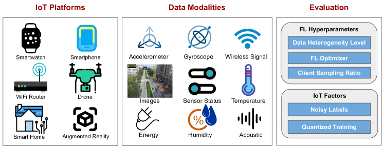
Refer to caption — Figure 1: Overview of FedAIoT.

In this paper, we present FedAIoT, an FL benchmark for AIoT. At its core, FedAIoT includes eight well-chosen datasets collected from a wide range of authentic IoT devices from smartwatch, smartphone and Wi-Fi routers, to drones, smart home sensors, and head-mounted device that either have already become an indispensable part of people’s daily lives or are driving emerging applications. These datasets encapsulate a variety of unique modalities from drone images and audios captured from head-mounted devices to wireless signals and smart home sensors that have not been explored in existing FL benchmarks. Moreover, these datasets target some of the most representative applications of AIoT as well as innovative use cases of AIoT that are not possible with other technologies.

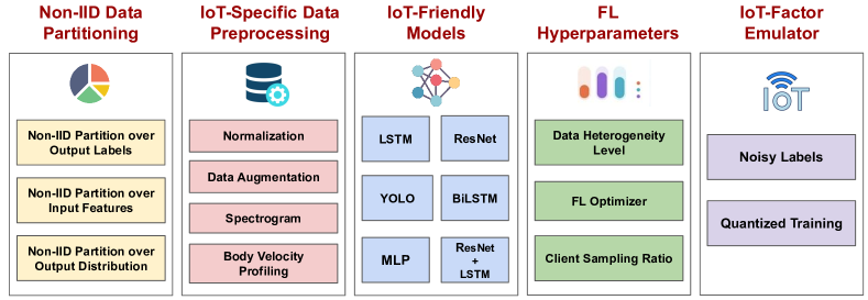
To facilitate the community benchmark the performance of the datasets and ensure reproducibility, FedAIoT includes a unified end-to-end FL framework for AIoT that covers the complete FL-for-AIoT pipeline: from non-IID data partitioning, data preprocessing, to AIoT-friendly models, FL hyperparameters, and IoT-factor emulator. Our framework also includes the implementations of popular schemes, models, and techniques involved in each stage of the FL-for-AIoT pipeline.

We have conducted a systematic benchmarking on the eight datasets using the end-to-end framework. Specifically, we examine the impact of varying degrees of non-IID data distributions, FL optimizers, and client sampling ratios on the performance of FL. We also evaluate the impact of erroneous labels, a prevalent challenge in IoT datasets, as well as the effects of quantized training, a technique that tackles the practical limitation of resource-constrained IoT devices. Our benchmark results provide valuable insights on both the opportunities and challenges of FL for AIoT. Given the significant relevance of FL in the realm of AIoT, we hope FedAIoT could act as a valuable tool to foster advancements in the important area of FL for AIoT.

2 Related Work

The importance of data to FL research pushes the development of FL benchmarks on a variety of data modalities. Existing FL benchmarks, however, predominantly center around curating federated datasets in the domain of computer vision (CV) [he2021fedcv, caldas2018leaf, Song2022FLAIRFL, lai2022fedscale, Dimitriadis2022FLUTEAS], natural language processing (NLP) [lin2021fednlp, caldas2018leaf, lai2022fedscale, Dimitriadis2022FLUTEAS], medical imaging [terrail2022flamby], speech and audio [zhang2023fedaudio, Dimitriadis2022FLUTEAS], and graph neural networks [he2021fedgraphnn]. For example, LEAF [caldas2018leaf] is one of the earliest FL benchmarks which comprises six datasets dedicated to CV and NLP; FedCV [he2021fedcv], FedNLP [lin2021fednlp], and FedAudio [zhang2023fedaudio] focuses on CV, NLP, and audio-related datasets and tasks respectively; FedScale [lai2022fedscale] provides an assortment of $20$ federated datasets mainly in CV and NLP applications, placing a distinct emphasis on system-related aspects; FLUTE [Dimitriadis2022FLUTEAS] covers a mix of datasets from CV, NLP, and audio; and FLamby [terrail2022flamby] presents seven healthcare-related datasets including five medical imaging datasets. Although these benchmarks have significantly contributed to FL research, a dedicated FL benchmark explicitly tailored for IoT data is absent. FedAIoT is specifically designed to fill this critical gap by providing a dedicated benchmark that focuses on data collected by a wide range of authentic IoT devices.

3 Design of FedAIoT

Table 1: Overview of the datasets included in FedAIoT.

Dataset	IoT Platform	Data Modality	Data Dimension	Dataset Size	# Training Samples	# Clients
WISDM-W [weiss2019wisdm]	Smartwatch	Accelerometer
Gyroscope	$200\times 6$	294 MB	$16,569$	80
WISDM-P [weiss2019wisdm]	Smartphone	Accelerometer
Gyroscope	$200\times 6$	253 MB	$13,714$	80
UT-HAR [yousefi2017uthar]	Wi-Fi Router	Wireless Signal	$3\times 30\times 250$	854 MB	$3,977$	20
Widar [zheng2020widardata, zheng2019zero]	Wi-Fi Router	Wireless Signal	$22\times 20\times 20$	3.3 GB	$11,372$	40
VisDrone [pengfei2021visdrone]	Drone	Images	$3\times 224\times 224$	1.8 GB	$6,471$	30
CASAS [schmitteredgecombe2009assesssing]	Smart Home	Motion Sensor
Door Sensor
Thermostat	$2000\times 1$	233 MB	$12,190$	60
AEP [candanedo2017datadriven]	Smart Home	Energy, Humidity
Temperature	$18\times 1$	12 MB	$15,788$	80
EPIC-SOUNDS [epicsounds2023, damen2022rescaling]	Augmented Reality	Acoustics	$400\times 128$	34 GB	$60,055$	210

3.1 Datasets

Table 1 provides an overview of the eight datasets included in FedAIoT. In this section, we provide a brief overview of each included dataset.

WISDM: The Wireless Sensor Data Mining (WISDM) dataset [weiss2019wisdm, wisdm2] is one of the widely used datasets for the task of daily activity recognition using accelerometer and gyroscope sensor data collected from smartphones and smartwatches. WISDM includes data collected from $51$ participants performing $18$ daily activities, each in a $3$ -minute session. We combined activities such as eating soup, chips, pasta, and sandwiches into a single category called "eating", and removed uncommon activities related to playing with balls, such as kicking, catching, or dribbling. We randomly selected $45$ participants as the training set and the rest of the $6$ participants were assigned to the test set. Given that in real-life settings individuals may not carry a smartphone and wear a smartwatch at the same time, we partition WISDM into two separate datasets: WISDM-W with smartwatch data only and WISDM-P with smartphone data only. The total number of samples in the training and test set is $16,569$ and $4,103$ for WISDP-W and $13,714$ and $4,073$ for WISDP-P respectively. No Licence was explicitly mentioned on the dataset homepage.

UT-HAR: The UT-HAR dataset [yousefi2017uthar] is a Wi-Fi dataset for the task of contactless activity recognition. The Wi-Fi data are in the form of Channel State Information (CSI) collected using three pairs of antennas and an Intel 5300 Network Interface Card (NIC), with each antenna pair capable of capturing $30$ subcarriers of CSI. UT-HAR comprises data collected from participants performing seven activities such as walking and running. UT-HAR contains a pre-determined training and test set. The total number of training and test samples is $3,977$ and $500$ respectively.

Widar: The Widar dataset [zheng2020widardata, zheng2019zero] is another Wi-Fi dataset but designed for the task of contactless gesture recognition. The Wi-Fi data are in the form of Wi-Fi signal strength measurements collected using Wi-Fi access points placed strategically in a room. The data collection system employs an Intel $5300$ NIC equipped with $3\times 3$ pairs of antennas. Widar contains data collected from $17$ participants performing $22$ distinct gestures including gestures such as push & pull, sweeping, clapping, and drawing various shapes and numbers. However, not all the gestures are uniformly represented across all users whereas some gestures were only performed by a single user. To ensure consistency between training and test sets, only those gestures that were recorded by more than three users are included in the experimental dataset. This yields a more balanced dataset, encompassing nine gestures with a total sample count of $11,372$ in the training set and $5,222$ in the test set. The dataset is under Creative Commons Attribution-NonCommercial 4.0 International Licence (CC BY 4).

VisDrone:

The VisDrone dataset [pengfei2021visdrone] is a large-scale dataset dedicated to the task of object detection in aerial images captured by drone cameras. VisDrone includes a total of $263$ video clips, containing in $179,264$ frames and $2,512,357$ labeled objects. The labeled objects fall into $12$ categories (e.g., ‘pedestrian’, ‘bicycle’, and ‘car’), recorded under a variety of scenarios such as crowded urban areas, highways, and parks. The dataset contains a pre-determined training and test set. The total number of samples in the training and test set is $6,471$ and $1,610$ respectively. The dataset is licenced under Creative Commons Attribution-NonCommercial-ShareAlike 3.0 License CASAS:

The CASAS dataset [schmitteredgecombe2009assesssing], derived from the CASAS smart home project, is a smart home sensor dataset for the task of recognizing activities of daily living (ADL) based on sequences of sensor states over time to support the application of independent living. The data were collected from three distinct apartments, each equipped with three types of sensors: motion sensors, temperature sensors, and door sensors. Five specific datasets, named ‘Milan’, ‘Cairo’, ‘Kyoto2’, ‘Kyoto3’, and ‘Kyoto4’, were selected based on the uniformity of their sensor data representation. The original activity classifications within each dataset have been consolidated into $11$ categories related to home activities such as Sleep, Eating, and Bathing. Activities not fitting within these categories were collectively classified as Other. The training and test set was made using an 80-20 split. Each data sample is a categorical time series of length $2,000$ , representing sensor states over a certain period of time. The total number of samples in the training and test set is $12,190$ and $3,048$ respectively. No Licence was explicitly mentioned on the dataset homepage.

AEP: The Appliances Energy Prediction (AEP) dataset [candanedo2017datadriven] is another smart home sensor dataset but designed for the task of predicting home energy usage. The data were collected from energy sensors, temperature sensors, and humidity sensors installed inside a home every $10$ minutes over $4.5$ months. The total number of samples in the training and test set is $15,788$ and $3,947$ respectively. No Licence was explicitly mentioned on the dataset homepage.

EPIC-SOUNDS: The EPIC-SOUNDS dataset [epicsounds2023] is a large-scale collection of audio recordings for the task of audio-based human activity recognition in Augmented Reality applications. The audio data were collected from a head-mounted microphone including more than $100$ k categorized segments distributed across $44$ distinct classes. The dataset contains a pre-determined training and test set. The total number of training and test samples is $60,055$ and $40,175$ respectively. The dataset is under CC BY 4 Licence.

3.2 End-to-End Federated Learning Framework for AIoT

To benchmark the performance of the datasets and facilitate future research in FL for AIoT, we have designed and developed an end-to-end FL framework for AIoT as another key part of FedAIoT. As illustrated in Figure 2, our framework covers the complete FL-for-AIoT pipeline, which includes five components: (1) non-IID data partitioning, (2) data preprocessing, (3) AIoT-friendly models, (4) FL hyperparameters, and (5) IoT-factor emulator. In this section, we describe each component within the framework in detail.

3.2.1 Non-IID Data Partitioning

The objective of non-IID data partitioning is to partition the training set such that data allocated to different clients follow the non-IID distribution. The eight datasets included in FedAIoT cover three fundamental tasks (classification, regression, object detection). FedAIoT incorporates three different non-IID data partitioning schemes that are designed for the three tasks respectively.

Scheme#1: Non-IID Partition over Output Labels. For the task of classification (WISDM-W, WISDM-P, UT-HAR, Widar, CASAS, EPIC-SOUNDS) with $C$ classes, we first generate a distribution over the classes for each client by drawing from a Dirichlet Distribution with parameter $\alpha$ [hsu2019measuring], where lower values of $\alpha$ generated more skewed distribution favoring a few classes whereas higher values of $\alpha$ result in more balanced class distribution. We use the same $\alpha$ to determine the number of samples each client receives. In addition, by drawing from a Dirichlet Distribution with parameter $\alpha$ , we create a distribution over the total number of samples, which is then used to allocate a varying number of samples to each client, where lower values of $\alpha$ lead to a few clients holding a majority of the samples whereas higher values of $\alpha$ create a more balanced distribution of samples across clients. This approach allows us to generate non-IID data partitions that better mimic real-world scenarios, where both the class distribution and the number of samples can vary across the clients.

Scheme#2: Non-IID Partition over Input Features. The task of object detection (VisDrone) does not have specific classes. In such cases, we use the input features to create non-IID partitions. Specifically, similar to [he2021fedcv], we first used ImageNet [russakovsky2015imagenet] features generated from a VGG19 model [liu2015vgg19], which encapsulate crucial visual information required for subsequent analysis. With these ImageNet features as inputs, we performed clustering in the feature space using $K$ -nearest neighbors to partition the dataset into ten distinct clusters. Each cluster is a pseudo-class, representing a set of images sharing common visual characteristics as per the extracted ImageNet features. Lastly, Dirichlet Allocation was subsequently applied on top of the pseudo-classes to create the non-IID distribution across different clients.

Scheme#3: Non-IID Partition over Output Distribution. For the task of regression (e.g., AEP dataset) where the output is characterized as a continuous variable, we utilize Quantile Binning, a technique that transforms a continuous variable into a categorical one. Specifically, we divide the range of the output variable into ten equal groups or quantiles, ensuring that each bin accommodates roughly the same number of samples. Each category or bin is treated as a pseudo-class. Once the continuous output has been converted into ten categories, we apply Dirichlet Allocation to generate a non-IID distribution of data across the clients.

3.2.2 Data Preprocessing

The eight datasets included in FedAIoT cover diverse data modalities. FedAIoT incorporates different data preprocessing techniques for different data modalities accordingly. Because of the diversity in sensor and data modality, pre-processing techniques need to be tailored accordingly to remove outliers and minimize noise.

WISDM: We followed the standard preprocessing techniques used in accelerometer and gyroscope-based activity recognition for WISDM. Specifically, for each $3$ -minute session, we used a $10$ -second sliding window with $50$ % overlap to extract samples from the raw accelerometer and gyroscope data sequences. We then normalize each dimension of the extracted samples by removing the mean and scaling to unit variance.

UT-HAR: We followed [yang2023sensefi] and applied a sliding window of $250$ packets with $50$ % overlap to the raw Wi-Fi data from all three antennas to extract samples. We then normalize each dimension of the extracted samples by removing the mean and scaling to unit variance.

Widar: We adopt the body velocity profile (BVP) processing technique as outlined in [yang2023sensefi, zheng2019zero] in order to effectively handle and remove environmental variations from the data. We then apply standard scalar normalization to further refine the data. This creates data samples with the shape ( $22\times 20\times 20$ ) reflecting time axis, $x$ , and $y$ velocity features respectively.

VisDrone: We first normalized the images within a range of 0 to 1 to standardize the pixel values. Data augmentation techniques including random shifts in Hue, Saturation, and Value color space, image compression, shearing transformations, scaling transformations, horizontal and vertical flipping, and MixUp were applied to increase the diversity and generalizability of the dataset.

CASAS: We followed [liciotti2019sequential] to transform the sensor readings into categorical sequences, creating a form of semantic encoding. Each unique temperature setting is assigned a distinct categorical value, as are individual instances of motion sensors and door sensors being activated. For each recorded activity, we then extract a sequence of the 2000 previous sensor activations which is used for modeling and prediction activity.

AEP: Temperature data were log-transformed for skewness, and ‘visibility’ was binarized. Outliers below the \nth10 or above the \nth90 percentile were replaced with corresponding percentile values. Central tendency and date features were added for time-related patterns. Principal component analysis was used for data reduction, and the output was normalized using a standard scaler.

EPIC-SOUNDS: We first performed Short-Time Fourier Transform on raw audio segments followed by applying a Hann window of 10ms duration and a step size of 5ms to ensure optimal spectral resolution. We then extracted $128$ Mel Spectrogram features, a popular choice for audio classification tasks due to their ability to mimic human auditory system characteristics. To further enhance the data, we applied a natural logarithm scaling to the Mel Spectrogram output. Lastly, to enforce uniform input size across all samples, we padded each segment to reach a consistent length of $400$ .

3.2.3 AIoT-friendly Models

Our choice of models is informed by a combination of state-of-the-art results, as referenced in [wisdmmodel, yang2023sensefi, terven2023comprehensive, liciotti2019sequential, seyedzadeh2018energy, sholahudin2016prediction, epicsounds2023], and the resource constraints of the IoT platforms. For example, it is unrealistic to assume that IoT platforms could load and run large Transformer-based models for FL. Hence, we focus on AIoT-friendly models in FedAIoT. Table 2 presents the list of the selected models. A detailed breakdown of each model’s architecture can be found in Appendix A.3. Furthermore, a list of models supported for each dataset is also provided in Appendix.

Table 2: Non-IID data partitioning schemes and models used for each dataset.

Dataset	WISDM-W	WISDM-P	UT-HAR	Widar	VisDrone	CASAS	AEP	EPIC-SOUNDS
Partition	Output Labels	Output Labels	Output Labels	Output Labels	Input Features	Output Labels	Output Distribution	Output Labels
Model	LSTM	LSTM	ResNet18	ResNet18	YOLOv8n	BiLSTM	MLP	ResNet18
	${}^{\cite[cite]{[\@@bibref{}{wisdmmodel}{}{}]}}$	${}^{\cite[cite]{[\@@bibref{}{wisdmmodel}{}{}]}}$	${}^{\cite[cite]{[\@@bibref{}{he2016residual, yang2023sensefi, hsieh2020data}{}{}]}}$	${}^{\cite[cite]{[\@@bibref{}{he2016residual, yang2023sensefi, hsieh2020data}{}{}]}}$	${}^{\cite[cite]{[\@@bibref{}{terven2023comprehensive}{}{}]}}$	${}^{\cite[cite]{[\@@bibref{}{liciotti2019sequential}{}{}]}}$	${}^{\cite[cite]{[\@@bibref{}{seyedzadeh2018energy}{}{}]}}$	${}^{\cite[cite]{[\@@bibref{}{epicsounds2023}{}{}]}}$

3.2.4 FL Hyperparameters

Data Heterogeneity Level. Non-IIDness is a fundamental challenge in FL training, creating artifacts like gradient drifting that negatively impact the final model performance. As outlined in Section 3.2.1, FedAIoT facilitates the creation of diverse data partitions, allowing for the simulation of varying levels of data heterogeneity to meet experimental requirements.

FL Optimizer. FedAIoT supports a handful of commonly used FL optimizers. In the experiment section, we showcase the benchmark results of two FL optimizers: FedAvg [mcmahan2017communication] and FedOPT [reddi2020adaptive].

Client Sampling Ratio. Client sampling ratio denotes the proportion of clients selected for local training in each round of FL. This hyperparameter plays a crucial role as it directly influences the computation and communication costs associated with FL training. FedAIoT facilitates the creation of diverse client sampling ratios and the examination of its impact on both model performance and convergence speed during FL training.

3.2.5 IoT Factors

Real-world Erroneous Label Emulation. Real-world FL deployments on IoT devices often encounter label noise resulting from various sources such as bias, skill differences, and labeling errors introduced by annotators. To effectively emulate label errors in FL, we propose augmenting the ground truth labels of a dataset with a confusion matrix, denoted as $Q$ . Here, $Q_{ij}$ represents the probability that the ground truth label $i$ is changed to a different label $j$ , i.e., $P(\hat{y}=j\mid y=i)$ . Unlike previous benchmark work [zhang2023fedaudio], where the confusion matrix $Q$ was randomly constructed, our approach involves constructing the confusion matrix based on centralized training results. Specifically, we determine the elements of $Q$ (i.e., $Q_{ij}$ ) by calculating the ratio of the number of samples labeled as $j$ by the centrally trained machine learning model to the total number of samples with the ground truth label $i$ . This construction method ensures that the confusion matrix accurately reflects the labeling patterns observed during centralized training. We employ the confusion matrix $Q$ as a guiding tool for generating error labels. To introduce different levels of erroneous label ratio $\epsilon$ , we randomly select the required number of data samples and apply the label changes based on the probabilities specified in the confusion matrix $Q$ . By incorporating such realistic label errors in our FL simulations, we aim to provide a more reliable evaluation of FL algorithms under challenging real-world conditions.

Quantized Training. IoT devices often operate under significant resource constraints. In such case, model quantization becomes essential. This technique, involving the reduction of numerical precision in computations and data of AI models, optimizes memory use and computational efficiency. In FedAIoT, we incorporate two levels of precision, full (float32) and half (float16). While prior research has predominantly focused on the application of quantization during inference, it becomes equally crucial to examine the implications of training models under quantized conditions in the task of FL. Our models were thus trained under both precision formats. The objective was to investigate the balance between computational efficiency and model accuracy. This understanding is key in navigating the resource constraints of IoT devices and enabling FL for AIoT.

4 Experiments and Analysis

We implemented FedAIoT using PyTorch [pytorch] and Ray [ray], and conducted our experiments on a combination 8 $\times$ NVIDIA A6000 GPU cluster, 8 $\times$ NVIDIA RTX8000 GPU, 8 $\times$ NVIDIA A6000 GPU, 8 $\times$ NVIDIA RTX3090 GPU and 10 $\times$ NVIDIA A100 GPU clusters as needed.

4.1 Overall Performance

First, we benchmark the FL performance under two FL optimizers, FedAvg and FedOPT, under low ( $\alpha=0.5$ ) and high ( $\alpha=0.1$ ) data heterogeneity levels, and compare it against centralized training.

Table 3: Overall performance.

Dataset	Metric	Centralized	Low Data Heterogeneity ( $\mathbf{\alpha=0.5}$ )		High Data Heterogeneity ( $\mathbf{\alpha=0.1}$ )
Dataset	Metric	Centralized	FedAvg	FedOPT	FedAvg	FedOPT
WISDM-W	Accuracy (%)	71.47	68.60	67.93	65.97	59.03
WISDM-P	Accuracy (%)	35.76	33.74	31.67	32.26	28.72
UT-HAR	Accuracy (%)	95.79	94.57	76.96	76.04	66.04
Widar	Accuracy (%)	61.14	60.19	59.83	54.95	50.32
VisDrone	MAP-50 (%)	35.50	34.04	32.40	31.55	29.39
CASAS	Accuracy (%)	86.24	73.26	72.27	70.72	69.80
AEP	$R^{2}$	0.58	0.51	0.48	0.41	0.39
EPIC-SOUNDS	Accuracy (%)	42.67	34.82	29.10	26.71	20.01

Benchmark Results: Table 3 summarizes our results. We make three observations. (1) Data heterogeneity level and FL optimizer have different impacts on different datasets. In particular, the performance of UT-HAR and Widar are very sensitive to the data heterogeneity level. In contrast, WISDM-P does not show noticeably accuracy difference under FedAvg at different data heterogeneity levels. (2) Under low data heterogeneity, FedAvg provides a more stable performance compared to FedOPT and consistently achieves performance closer to centralized training across diverse data modalities. (3) Compared to the other datasets, CASAS, AEP, and EPIC-SOUNDS have higher accuracy margins between centralized training and low data heterogeneity. This indicates the need for more advanced FL algorithms for CASAS, AEP, and EPIC-SOUNDS datasets.

4.2 Impact of Client Sampling Ratio

IoT devices usually have significant communication restrictions and hence the client sampling ratio is a critical hyperparameter for FL systems operating AIoT devices. In this experiment, we focus on two client sampling ratios: $10$ % and $30$ %. Our exploration involved recording the maximum accuracy reached after completing $50$ %, $80$ %, and $100$ % of the total training rounds for both these ratios under high data heterogeneity, thereby offering empirical evidence of how the model’s performance and convergence rate are affected by the client sampling ratio.

Table 4: Impact of client sampling ratio.

Dataset	Training Rounds	Low Client Sampling Ratio ( $10\%$ )			High Client Sampling Ratio ( $30\%$ )
Dataset	Training Rounds	50% Rounds	80% Rounds	100% Rounds	50% Rounds	80% Rounds	100% Rounds
WISDM-W	400	57.15	63.40	65.97	59.17	65.85	66.78
WISDM-P	400	32.26	32.26	32.26	31.05	32.73	32.73
UT-HAR	1200	53.3	71.46	76.04	60.12	77.92	81.67
Widar	900	47.09	54.91	54.94	37.69	51.88	55.25
VisDrone	600	30.61	31.55	31.55	33.02	35.80	35.80
CASAS	400	70.72	70.72	70.72	75.13	76.05	76.68
AEP	2000	0.39	0.40	0.41	0.51	0.52	0.53
EPIC-SOUNDS	400	16.28	23.93	26.71	15.54	24.01	26.87

Benchmark Results: Table 4 summarizes our results. We make two observations. (1) An increased client sampling ratio is highly correlated with superior model accuracy (i.e., highest accuracy within 100% training rounds) across different IoT data modalities. This demonstrates the importance of the client sampling ratio to the final model performance at the end of FL. (2) However, a higher sampling ratio does not inherently guarantee faster model convergence. For example, WISDM-P, Widar, and EPIC-SOUNDS achieve higher model performance with a lower client sampling ratio at 50% training rounds compared to a higher client sampling ratio. This result underscores the complex dynamics between client participation and learning efficiency for different IoT data modalities.

4.3 Impact of Erroneous Labels

As elaborated in Section 3.2.5, we investigate the implications of erroneous labels. We assess the performance of our models under circumstances where the label error ratio is set at $10$ % and $30$ %, juxtaposing these results with the control scenario that involves no label errors. Note that we only showcase this for ‘WISDM’, ‘UT-HAR’, ‘WIDAR’, ‘CASAS’, and ‘EPIC-SOUNDS’ as these are classification tasks, and the concept of erroneous labels only apply to classification tasks.

Table 5: Impact of erroneous labels.

Benchmark Results: Table 4.3 summarizes our results. We make two observations. (1) As the ratio of erroneous labels increases, the performance of the models decreases across all the datasets, and the impact of erroneous labels varies across different datasets. For example, WISDM-W only experiences a little performance drop at $10$ % label error ratio, but its performance significantly drops when the label error ratio increases to $30$ %. In contrast, CASAS exhibits a more gradual decline in performance as the error ratio increases from $0$ % to $10$ % and from $10$ % to $30$ %. (2) UT-HAR and EPIC-SOUNDS are very sensitive to label error and show significant accuracy drop even at $10$ % label error ratio.

4.4 Performance on Quantized Training

Lastly, we examine the impact of model quantization on federated learning, specifically using half-precision (FP16). We assess the models’ accuracy and memory usage under this quantization, comparing these results to those from the full-precision (FP32) models. Memory is measured by analyzing the GPU memory usage of a model when trained with the same batch size under a centralized setting.

Table 6: Performance on quantized training.

Dataset	Metric	FP32		FP16
Dataset	Metric	Model Performance	Memory Usage	Model Performance	Memory Usage
WISDM-W	Accuracy (%)	65.97	1444 MB	65.97	564 MB ( $\downarrow$ 60.9%)
WISDM-P	Accuracy (%)	32.26	1444 MB	31.91	564 MB ( $\downarrow$ 60.9%)
UT-HAR	Accuracy (%)	76.04	1716 MB	72.06	639 MB ( $\downarrow$ 62.8%)
Widar	Accuracy (%)	54.95	1734 MB	39.55	636 MB ( $\downarrow$ 63.3%)
VisDrone	MAP-50 (%)	32.09	8369 MB	24.07	3515 MB ( $\downarrow$ 60.0%)
CASAS	Accuracy (%)	70.72	1834 MB	77.99	732 MB ( $\downarrow$ 60.1%)
AEP	$R^{2}$	0.41	1201 MB	0.279	500 MB ( $\downarrow$ 58.4%)
EPIC-SOUNDS	Accuracy (%)	26.71	2176 MB	27.88	936 MB ( $\downarrow$ 57.0%)

Benchmark Results: Table 6 summarizes the model performance and memory usage at two precision levels. We make three observations: (1) As expected, the memory usage significantly decreases when using FP16 precision, ranging from $57.0$ % to $63.3$ % reduction across different datasets. (2) As shown in the previous work [Micikevicius2017MixedPT], the model performance associated with the precision levels varies depending on the dataset. For WISDM-W, CASAS, and EPIC-SOUNDS, the FP16 models maintain or even improve the performance compared to the FP32 models. (3) Widar, VisDrone, and AEP have a significant decline in performance when quantized to FP16 precision.

Table 7: Analysis of quantization demands.

Application	Dataset	IoT Platform	Representative Devices	Hardware RAM Size	Need Quantization
Activity Recognition	WISDM-W	Smartwatch	Apple Watch 8	512 MB to 1 GB	Yes
	WISDM-P	Smartphone	iPhone 14	6 GB	No
	UT-HAR	Wi-Fi Router	TP-Link AX1800	64 MB to 1 GB	Yes
Gesture Recognition	Widar	Wi-Fi Router	TP-Link AX1800	64 MB to 1 GB	Yes
Independent Living	CASAS	Smart Home	Raspberry Pi 4	1 GB to 8 GB	No
Energy Prediction	AEP	Smart Home	Raspberry Pi 4	1 GB to 8 GB	No
Objective Detection	VisDrone	Drone	Dji Mavic 3 + Raspberry Pi 4	1 GB to 8 GB	Yes
Augmented Reality	EPIC-SOUNDS	Head-mounted Device	GoPro / AR Headset	1 GB to 8 GB	No

4.5 Insights from Benchmark Results

Need for Resilience on High Data Heterogeneity: As presented in Table 3, datasets can exhibit a notable response to changes in data heterogeneity. We observe that CASAS, AEP, and EPIC-SOUNDS show a significant impact even at a low data heterogeneity. UT-HAR and Widar see a drastic decline in high data heterogeneity. These findings emphasize the need for developing advanced FL algorithms for data modalities that are sensitive to high data heterogeneity.

Need for Balancing between Client Sampling Ratio and Resource Consumption of IoT Devices: Table 4 reveals that a higher sampling ratio can lead to improved performance in the long run. However, higher client sampling ratios generally entail increased communication bandwidth and energy consumption, which may not be desirable for IoT devices. Therefore, it is crucial to identify the sweet spot that strikes a balance between the client sampling ratio and resource consumption.

Need for Resilience on Erroneous Labels: As demonstrated in Table 4.3, certain datasets exhibit high sensitivity to label errors, resulting in a significant drop in FL performance. Notably, both UT-HAR and EPIC-SOUNDS experience a drastic decrease in accuracy when faced with a 10% erroneous label ratio. Given the inevitability of label errors in real FL deployments, where private data remains unmonitored and uncalibrated except by the respective data owners, the development of label error resilient techniques becomes crucial for achieving reliable FL performance.

Need for Quantization: Table 7 highlights the importance of quantization in FL for all eight datasets. Notably, certain IoT devices, such as drones, lack sufficient RAM storage capacity for FL. Hence, external hardware interfaces like Raspberry Pi 4 has to be incorporated as assistive computing platforms. Analysis from Table 6 reveals that the performance of VisDrone drops significantly from 32FP precision to 16FP precision, and WISDM-W, UT-HAR, and VisDrone require computing memory size that exceeds the representative hardware RAM limits when using 32FP precision, underscoring the necessity of quantized training.

5 Conclusion

In this paper, we presented FedAIoT, a FL benchmark for AIoT. FedAIoT includes eight datasets collected from a wide range of authentic IoT devices as well as a unified end-to-end FL framework for AIoT that covers the complete FL-for-AIoT pipeline. We have benchmarked the performance of the datasets and provided insights on the opportunities and challenges of FL for AIoT.

Limitations and Future works. While the benchmark presented is instrumental in elucidating the role of different factors on model accuracy, the scope of AIoT extends further. A holistic understanding of AIoT also necessitates an examination of its infrastructural facets. These encompass the computational prowess and energy utilization of IoT platforms, along with the efficiency and security of their communication protocols, which are equally vital dimensions in the AIoT landscape. Moving forward, our plan is to establish an open-source repository that hosts and maintains this benchmark. This endeavor will be guided by the invaluable insights we receive from the broader community and users of the benchmark framework. As a part of our ongoing commitment, we intend to continually expand the benchmark’s scope by incorporating additional datasets from a more diverse set of applications, integrating new algorithms, and conducting deeper analytical validations.

Checklist

1.
For all authors…
1. (a)
  
  Do the main claims made in the abstract and introduction accurately reflect the paper’s contributions and scope? \answerYes
2. (b)
  
  Did you describe the limitations of your work? \answerYes
3. (c)
  
  Did you discuss any potential negative societal impacts of your work? \answerNA
4. (d)
  
  Have you read the ethics review guidelines and ensured that your paper conforms to them? \answerYes
2.
If you are including theoretical results…
1. (a)
  
  Did you state the full set of assumptions of all theoretical results? \answerNA
2. (b)
  
  Did you include complete proofs of all theoretical results? \answerNA
3.
If you ran experiments (e.g. for benchmarks)…
1. (a)
  
  Did you include the code, data, and instructions needed to reproduce the main experimental results (either in the supplemental material or as a URL)? \answerYes
2. (b)
  
  Did you specify all the training details (e.g., data splits, hyperparameters, how they were chosen)? \answerYes
3. (c)
  
  Did you report error bars (e.g., with respect to the random seed after running experiments multiple times)? \answerNA
4. (d)
  
  Did you include the total amount of compute and the type of resources used (e.g., type of GPUs, internal cluster, or cloud provider)? \answerYes
4.
If you are using existing assets (e.g., code, data, models) or curating/releasing new assets…
1. (a)
  
  If your work uses existing assets, did you cite the creators? \answerYes
2. (b)
  
  Did you mention the license of the assets? \answerYesMentioned when available
3. (c)
  
  Did you include any new assets either in the supplemental material or as a URL? \answerYes
4. (d)
  
  Did you discuss whether and how consent was obtained from people whose data you’re using/curating? \answerNA
5. (e)
  
  Did you discuss whether the data you are using/curating contains personally identifiable information or offensive content? \answerNA
5.
If you used crowdsourcing or conducted research with human subjects…
1. (a)
  
  Did you include the full text of instructions given to participants and screenshots, if applicable? \answerNA
2. (b)
  
  Did you describe any potential participant risks, with links to Institutional Review Board (IRB) approvals, if applicable? \answerNA
3. (c)
  
  Did you include the estimated hourly wage paid to participants and the total amount spent on participant compensation? \answerNA

Appendix A Appendix

A.1 Supplementary Dataset Details

A.1.1 WISDM

The WISDM dataset comprises raw accelerometer and gyroscope data collected from 51 subjects performing 18 activities for three minutes each. Data were gathered at a 20Hz sampling rate from both a smartphone (Google Nexus 5/5x or Samsung Galaxy S5) and a smartwatch (LG G Watch). Data for each device and sensor type are stored in different directories, resulting in four directories overall. Each directory contains 51 files, each corresponding to a subject. The data entry format is: <subject-id, activity-code, timestamp, x, y, z>. Separate files for the gyroscope and accelerometer readings are provided and are later combined by matching timestamps. Subject ID is given from 1600 to 1650 and the activity code is an alphabetical character between ‘A’ and ‘S’ excluding ‘N’. The timestamp is in Unix time. The code to read and partition the data into 10s segments is provided by our benchmark. The input shape of the processed data is $200\times 6$ . The original dataset is available at https://archive.ics.uci.edu/dataset/507/wisdm+smartphone+and+smartwatch+activity+and+biometrics+dataset.

A.1.2 UT-HAR

The UT-HAR dataset was collected using the Linux 802.11n Channel State Information (CSI) Tool for the task of Human Activity Recognition (HAR). The original data consist of two file types: “input" and “annotation". “input" files contain Wi-Fi CSI data. The first column indicates the timestamp in Unix. Columns 2-91 represent amplitude data for 30 subcarriers across three antennas, and columns 92-181 contain the corresponding phase information. “annotation" files provide the corresponding activity labels, serving as the ground truth for HAR. In our benchmark, only amplitude is used. The final samples are created by taking a sliding window of size $250$ where each sample consists of amplitude information across three antennas and from 30 subcarriers and has shape $3\times 30\times 250$ . The original dataset is available at https://github.com/ermongroup/Wifi_Activity_Recognition/tree/master.

A.1.3 Widar

The Widar dataset (Widar3.0) was collected with a system comprising one transmitter and three receivers, all equipped with Intel 5300 wireless NICs. The system uses the Linux CSI Tool to record the Wi-Fi data. Devices operate in monitor mode on channel 165 at 5.825 GHz. The transmitter broadcasts $1,000$ Wi-Fi packets per second while receivers capture data using their three linearly arranged antennas. In our benchmark, we use the processed body velocity profile (BVP) features extracted from the dataset. The size of each data sample after processing is $22\times 20\times 20$ consisting of $22$ samples over time each having $20$ BVP features each in both $x$ and $y$ directions. The raw dataset is available for download at http://tns.thss.tsinghua.edu.cn/widar3.0/index.html.

A.1.4 VisDrone

The VisDrone dataset was collected by the AISKYEYE team at Tianjin University, China. It comprises 288 video clips with 261,908 frames and 10,209 static images captured by cameras mounted on drones at 14 different cities in China in diverse environments, scenarios, weather, and lighting conditions. The frames were manually annotated with over 2.6 million bounding boxes of common targets like pedestrians, cars, and bicycles. Additional attributes like scene visibility, object class, and occlusion are also provided for enhanced data utilization. The dataset is available at https://github.com/VisDrone/VisDrone-Dataset.

A.1.5 CASAS

The CASAS dataset is a collection of data generated in smart home environments, where intelligent software uses sensors deployed at homes to monitor resident activities and conditions within the space. The CASAS project considers environments as intelligent agents and employs custom IoT hardware known as Smart Home in a Box (SHiB), which encompasses the necessary sensors, devices, and software. The sensors in SHiB perceive the status of residents and their surroundings, and through controllers, the system acts to enhance living conditions by optimizing comfort, safety, and productivity. The CASAS dataset includes the date (in yyyy-mm-dd format), time (in hh:mm:ss.ms format), sensor name, sensor readings, and an activity label in string format. The data were collected in real-time as residents go about their daily activities. The code to extract categorical sensor readings to create input sequences and labels is provided in our benchmark. The CASAS dataset can be downloaded from https://casas.wsu.edu/datasets/.

A.1.6 AEP

The AEP dataset, collected over 4.5 months, comprises readings taken every 10 minutes from a ZigBee wireless sensor network monitoring house temperature and humidity. Each wireless node transmitted data around every 3.3 minutes, which were then averaged over 10-minute periods. Additionally, energy data was logged every 10 minutes via m-bus energy meters. The dataset includes attributes such as date and time (in year-month-day hour:minute:second format), the energy usage of appliances and lights (in Wh), temperature and humidity in various rooms including the kitchen ( $T_{1}$ , $RH_{1}$ ), living room ( $T_{2}$ , $RH_{2}$ ), laundry room ( $T_{3}$ , $RH_{3}$ ), office room ( $T4$ , $RH_{4}$ ), bathroom ( $T_{5}$ , $RH_{5}$ ), ironing room ( $T_{7}$ , $RH_{7}$ ), teenager room ( $T_{8}$ , $RH_{8}$ ), and parents room ( $T_{9}$ , $RH_{9}$ ), and temperature and humidity outside the building ( $T_{6}$ , $RH_{6}$ ) - all with temperatures in Celsius and humidity in percentages. Additionally, weather data from Chievres Airport, Belgium was incorporated, consisting of outside temperature (To in Celsius), pressure (in mm Hg), humidity ( $RH_{out}$ in %), wind speed (in m/s), visibility (in km), and dew point ( $T_{dewpoint}$ in °C). The dataset is available at https://archive.ics.uci.edu/dataset/374/appliances+energy+prediction.

A.1.7 EPIC-SOUNDS

As an extension of the EPIC-KITCHENS-100 dataset, the EPIC-SOUNDS dataset focuses on annotating distinct audio events in the videos of EPIC-KITCHENS-100. The annotations include the time intervals during which each audio event occurs, along with a text description explaining the nature of the sound. Given the variation in video lengths in the dataset, which range from 30 seconds to 1.5 hours, the videos are segmented into clips of 3-4 minutes each to make the annotation process more manageable. In order to ensure that annotators concentrate solely on the audio aspects, only the audio stream is provided to them. This decision is taken to prevent bias that could be introduced by the visual and contextual elements in the videos. Additionally, annotators are given access to the plotted audio waveforms. These visual representations of the audio data help the annotators by guiding them in pinpointing specific sound patterns, thus making the annotation process more efficient and targeted. The EPIC-SOUNDS dataset can be extracted from the EPIC-KITHENS-100 dataset with the GitHub repo at https://github.com/epic-kitchens/epic-sounds-annotations. The extracted audio data in the form of HDF5 file format can also be requested from uob-epic-kitchens@bristol.ac.uk.

A.2 Hyperparameters

Hyperparameters for Table 3. For WISDM-W, the learning rate for centralized training was 0.01 and we trained for 200 epochs with batch size 64. For FedAvg, in both low and high data heterogeneity scenarios, we used a client learning rate of 0.01 and trained for 400 communication rounds with batch size 32. For FedOPT, in both low and high data heterogeneity scenarios, we used a client learning rate of 0.01 and a server learning rate of 0.01. We also trained for 400 communication rounds. For WISDM-P, the learning rate for centralized training was 0.01 and we trained for 200 epochs with batch size 128. For FedAvg, in both low and high data heterogeneity scenarios, we used a client learning rate of 0.008 and trained for 400 communication rounds with batch size 32. For FedOPT, in both low and high data heterogeneity scenarios, we used a client learning rate of 0.01 and a server learning rate of 0.01. We also trained for 400 communication rounds. For UT-HAR and Widar, the learning rate for centralized training was 0.001 and the number of epochs was 500 and 200 for UT-HAR and Widar respectively with a batch size of 32. For both low and high data heterogeneity in both FedAvg and FedOPT, the client learning rate was 0.01 and the server learning rate for FedAvg and FedOPT was 1 and 0.01 respectively. The number of communication rounds was 1200 and 900 for UT-HAR and Widar respectively with a batch size of 32. For VisDrone, we used a cosine learning rate scheduler with $T_{0}=10,T_{mult}=2$ and trained for 200 epochs with a learning rate of 0.1 and batch size 12. For all the experiments on VisDrone, the client learning rate was also 0.1 and the batch size was 12. For FedOPT, the server learning rate was 0.1. For CASAS, the centralized learning rate was 0.1 with batch size 128. For the federated setting, the client learning rate was 0.005, and the batch size was 32. We trained for 400 rounds. For FedOPT, the server learning rate was 0.01. For AEP, the learning rate for centralized training was 0.001 and the batch size was 32 and it was trained for 1200 epochs. For federated experiments, the client learning rate was 0.01, and the batch size was 32. For FedOPT, the server learning rate was 0.1. For EPIC-SOUNDS, for centralized training, the learning rate was 0.1 with batch size 512. The number of epochs was 120. For federated settings, we used a client learning rate of 0.1 and batch size 32. For FedOPT, the server learning rate was 0.01.

Hyperparameters for Table 4. The setup for all the datasets with $10$ % client sampling rate is the same as that of Table 3 under high data heterogeneity. For the $30$ % client sampling rate, the hyperparameters were kept the same as that of the $10$ % client sampling rate experiments, with the exception of CASAS, where the learning rate was set to 0.15.

Hyperparameters for Table 4.3. The hyperparameters were the same as that of Table 3 with $10$ % sampling rate under high data heterogeneity scenario.

Hyperparameters for Table 6. The hyperparameters were same as that of Table 3 with $10$ % client sampling rate under high data heterogeneity scenario.

A.3 Model Architectures

A.3.1 WISDM

For WISDM, we use a custom LSTM model that consists of an LSTM layer followed by a feed-forward neural network. The LSTM layer has an input dimension of 6 and a hidden dimension of 6. After the LSTM layer, the output is flattened and passed through a dropout layer with a rate of 0.2 for regularization. It then goes through a fully connected linear layer with an input size of $1,200$ (6 hidden units * 200 timesteps) and an output size of 128, followed by a ReLU activation function. Another dropout layer with a rate of 0.2 is applied before the final fully connected linear layer with an input size of 128 and an output size of 12.

A.3.2 UT-HAR

For UT-HAR, we use a ResNet-18 model with custom architecture designed for the Wi-Fi based Human Activity Recognition (HAR) task. The model consists of an initial convolutional layer that reshapes the input into a 3-channel tensor followed by the main ResNet architecture with 18 layers. This main architecture includes a series of convolutional blocks with residual connections, Group Normalization layers, ReLU activations, and max-pooling. Finally, there is an adaptive average pooling layer followed by a fully connected layer that outputs the class probabilities. The model utilizes 64 output channels in the initial layer and doubles the number of channels as it goes deeper. The last fully connected layer has 7 output units corresponding to the number of classes for the UT-HAR task.

A.3.3 Widar

For Widar, we also use a custom ResNet-18 model tailored for the Widar dataset. The model starts by reshaping the 22-channel input to 3 channels using two convolutional transpose layers, followed by a convolutional layer with 64 filters, Group Normalization, ReLU activation, and max-pooling. The core of the model consists of four layers of residual blocks (similar to the standard ResNet18) with 64, 128, 256, and 512 filters. Each basic block within these layers contains two convolutional layers, Group Normalization, and ReLU activations. Finally, an adaptive average pooling layer reduces spatial dimensions to $1\times 1$ , followed by a fully connected layer to output class scores.

A.3.4 VisDrone

For VisDrone, we use the default YOLOv8n model from Ultralytics library. YOLOv8n is the smallest YOLOv8 model variant with the three scale parameters: depth, width, and the maximum number of channels set to 0.33, 0.25, and 1024 respectively.

A.3.5 CASAS

For CASAS, we use a BiLSTM neural network which is composed of an embedding layer, a bidirectional LSTM, and a fully connected layer. The embedding layer takes input sequences with dimensions equal to the input dimension and converts them to dense vectors of size 64. The bidirectional LSTM layer has an input size equal to 64, the same number of hidden units, and processes the embedded sequences in both forward and backward directions. The output of the LSTM layer is connected to a fully connected layer with an input size of 128 (to account for the bidirectional LSTM concatenation) and outputs the logits for 12 activities in the CASAS dataset.

A.3.6 AEP

For AEP, we use a custom multi-layer perceptron (MLP) neural network with an architecture comprising five hidden layers and an output layer. The input layer accepts 18 features and passes them through a linear transformation to the first hidden layer with 210 units. Each of the following hidden layers progressively scales the number of units by factors of 2 and 4 and then scales down. Specifically, the sizes of the hidden layers are 210, 420, 840, 420, and 210 units respectively. Each hidden layer uses a ReLU activation function followed by a dropout layer with a dropout rate of 0.3 for regularization. The output layer has a single unit, and the output of the network is obtained by passing the activations of the last hidden layer through a final linear transformation.

A.3.7 EPIC-SOUNDS

For EPIC-SOUNDS, we again use a custom ResNet-18 model which consists of a stack of convolutional layers followed by batch normalization and ReLU activation. The architecture begins with a $7\times 7$ convolutional layer with stride 2, followed by a max pooling layer. Then, it contains four blocks, each comprising a sequence of basic blocks with a residual connection; specifically, each block contains two basic blocks, with output channel sizes of 64, 128, 256, and 512 respectively. Each basic block comprises two sets of 3x3 convolutional layers, each followed by batch normalization and ReLU activation. The first convolutional layer in the basic block has a stride of 2 in the second, third, and fourth blocks. Finally, the model has an adaptive average pooling layer, which reduces the spatial dimensions to 1x1, followed by a fully connected layer with an output size of 44 classes.