Linear classification methods for multivariate repeated measures data - a simulation study

Abstract

Researchers in the behavioral and social sciences often use linear discriminant analysis (LDA) for predictions of group membership (classification) and for identifying the variables most relevant to group separation among a set of continuous correlated variables (description). In this paper, we compare existing linear classification algorithms for nonnormally distributed multivariate repeated measures data in a simulation study based on Likert-type data.
It is widely accepted that, as a multivariate technique, LDA provides more accurate results by examining not only the relationship between the independent and dependent variables but also the relationships within the independent variables themselves. In educational and psychological research and other disciplines, longitudinal data are often collected which provide additional temporal information. However, linear classification methods for repeated measures data are rarely discussed in the literature despite these potential applications. These methods are more sensitive to actual group differences by taking the complex correlations between time points and variables into account, when compared to analyzing the data at each time point separately. Moreover, data in the behavioral and social sciences rarely fulfill the multivariate normality assumption, so we consider techniques that additionally do not require multivariate normality.
The results show that methods which include multivariate outlier removal before parameter estimation as well as robust parameter estimation using generalized estimating equations (GEE) perform better than the standard repeated measures LDA which assumes multivariate normality. The results of the longitudinal support vector machine (SVM) were not competitive.

1 Introduction

In psychology and the social sciences, discriminant analysis (DA) is traditionally applied to classification tasks in data with continuous variables since its invention by Fisher (1936). Its importance for the behavioral sciences has often been emphasized in reviews, tutorials and textbooks (Boedeker and Kearns, 2019; Sherry, 2006; Field, 2017; Huberty and Olejnik, 2006; Fletcher et al, 1978; Betz, 1987; Garrett, 1943). It has been applied to a large number of problems in experimental and applied psychology for class prediction as well as description (Rogge and Bradbury, 1999; Langlois et al, 2000; O’Brien et al, 2009; Kumpulainen et al, 2021; Shinba et al, 2021; Stoyanov et al, 2022; Aggarwala et al, 2022).
Longitudinal data are collected in various disciplines since they provide additional information about temporal changes. Longitudinal studies in psychology and the social sciences (Jensen et al, 2021; Banks et al, 2021; McLanahan et al, 2019) provide potential applications for repeated measures DA or alternative linear classification techniques. At the same time, textbooks discussing DA do not mention respective repeated measures approaches (Lix and Sajobi, 2010).
Traditional classification approaches for continuous multivariate repeated measures data typically assume multivariate normality (Roy and Khattree, 2005a, b; Tomasko et al, 2010; Gupta, 1986), but this assumption is rarely fulfilled by psychological datasets and hard to verify for small sample sizes (Delacre et al, 2017; Rausch and Kelley, 2009; Beaumont et al, 2006; Neto et al, 2016). Psychological data, especially those obtained using patient-reported instruments, are often characterized by skewness.
There are only few alternative approaches which relax or overcome the multivariate normality assumption and take the complex correlation structure between time points and variables into account. We consider the modifications of repeated measures LDA by Brobbey et al. (2021; 2022) that are more robust to deviations from multivariate normality. In their work, they compare the performance of the standard repeated measures LDA (which is based on the unstructured pooled covariance matrix estimate) once to its performance with preceding multivariate outlier removal using two different trimming algorithms by Rousseeuw (1985), and once to its performance when the covariance is estimated by a parsimonious Kronecker product structure using the generalized estimating equations (GEE) model (Inan, 2015), respectively. In both cases, comparisons are made for a number of different simulation scenarios but data are always simulated assuming a parsimonious Kronecker structure for group means and covariance matrices, respectively, and correlations between variables that remain constant over time. Furthermore, the two robust methods are not compared among each other. We furthermore consider the generalization of the support vector machine classifier by Chen and Bowman (2011) to longitudinal data which uses a weighted combination of multivariate measurements taken at several time points as input. This longitudinal SVM, when used with a linear kernel, can also be used as a descriptive method, since it provides a weight vector corresponding to the variables’ relative importance for separating the classes similar to Fisher discriminant function coefficients in DA.
In this paper, we are trying to mimick realistic datasets. We base simulations on unstructured means and covariance matrices estimated from psychometric reference datasets which differ in sample sizes, sample size ratios, class overlap, temporal variation and number of measurement occasions.
In our simulations, we compare the performance of the standard repeated measures LDA with the performance of repeated measures LDA based on GEE estimates by Brobbey et al. (2022), the repeated measures LDA when estimating the parsimonious Kronecker product covariance and the longitudinal SVM, each time either without or with preceding application of one of the two trimming algorithms as proposed by Brobbey (2021). In this way, we compare all potential combinations of these classification procedures applicable to linear classification problems of multivariate repeated measures data and evaluate their performance in data which deviate from multivariate normality. Furthermore, we evaluate the algorithms’ performance in the reference data using a nonparametric bootstrap approach which estimates confidence intervals for the point estimates (Wahl et al, 2016).
The paper is organized as follows. In Section 2, we describe the methods, i.e. the bootstrap approach proposed by Wahl et al. (2016) as well as the robust or nonparametric linear classification procedures, describe the reference datasets and the simulation setup. In Section 3, we present and discuss the results and provide recommendations based on the findings. Conclusions are made in Section 4.

2 Data and Methods

In this section, we will describe the traditional repeated measures LDA, its robust versions and the nonparametric longitudinal SVM for classification of nonnormally distributed repeated measures data. We consider a situation with a categorical outcome variable $i\in\{0,1\}$ (corresponding to two distinct groups) and $n=n_{0}+n_{1}$ samples, where measurements of $p$ variables are taken at $t$ consecutive time points. We consider complete data, i.e. for each individual $j\in\{1,\dots,n_{i}\}$, each measurement $l=1,\dots,p$ is taken at each time point $k=1,\dots,t$.
Table 1 gives an overview of the considered methods. Furthermore, we describe the nonparamtric bootstrap approach for estimation of the methods’ performance in the original data (Wahl et al, 2016), the simulation setup and the reference datasets.

Table 1: Overview of the considered linear classification methods for nonnormally distributed multivariate repeated measures data. The performance of each classification method is estimated either without or in combination with preceding multivariate outlier removal (using the Minimum Volume Ellipsoid (MVE) or the Minimum Covariance Determinant (MCD) algorithm, respectively).

Linear classification method	Description
Repeated measures linear discriminant analysis (LDA) 1)   standard/traditional 2)   robust	Parametric method depending on estimates of the group means and common covariance matrix (unstructured) pooled covariance matrix a)   (parsimonious) Kronecker product covariance estimated by flip-flop algorithm b) (unstructured) covariance matrix estimated using the joint Generalized Estimating Equations model
Longitudinal Support Vector Machine (SVM) using a linear kernel	Nonparametric method independent of distributional assumptions

2 .1 Multivariate repeated measures LDA

For LDA, the unknown parameters $\bm{\mu}_{i}\in\mathds{R}^{pt}$, the group-specific mean vectors, and $\bm{\Sigma}\in\mathds{R}^{pt\times pt}$, the common covariance matrix, need to be estimated from the data. The covariance matrix $\bm{\Sigma}$ is assumed to be positive definite. Assuming that $\bm{\Sigma}$ is unstructured, all distinct correlations between each pair of the $p$ variables and each combination of the $t$ time points must be estimated. If the dataset is small, the estimate $\widehat{\bm{\Sigma}}$ may become singular, i.e. if $n\leq pt$. In order to reduce the complexity of $\bm{\Sigma}$ or to estimate $\bm{\Sigma}$ more efficiently, a reduced number of parameters can be considered by assuming, for example, a Kronecker product structure $\bm{\Sigma}=\bm{\Sigma}_{t\times t}\otimes\bm{\Sigma}_{p\times p}$. Here, $\bm{\Sigma}_{t\times t}\in\mathds{R}^{t\times t}$ comprises the correlations between the $t$ time points and $\bm{\Sigma}_{p\times p}\in\mathds{R}^{p\times p}$ comprises the correlations between the $p$ variables. The number of unknown parameters reduces from $(pt(pt+1)/2)$ for an unstructured covariance matrix to $p(p+1)/2+t(t+1)/2$ for a Kronecker product covariance matrix (Naik and Rao, 2001). It can be estimated by the flip-flop algorithm, which gives maximum likelihood estimates of $\bm{\Sigma}_{t\times t}$ and $\bm{\Sigma}_{p\times p}$ (Lu and Zimmerman, 2005). The flip-flop algorithm is suitable in case the entries in the vector of observations $\textbf{x}\in\mathds{R}^{pt}$ can be separated with respect to two factors, which are the time points and variables in case of multivariate longitudinal data.
Brobbey et al. (2021; 2022) developed two approaches for robust LDA based on the Kronecker product estimate of the covariance matrix that will be described in the following.
The LDA classification rule states that a new observation $\textbf{x}\in\mathds{R}^{pt}$ is assigned to class 0 if

$$\left(\textbf{x}-\frac{\bm{\mu}_{0}+\bm{\mu}_{1}}{2}\right)^{T}\bm{\Sigma}^{-1}(\bm{\mu}_{0}-\bm{\mu}_{1})>\log\left(\frac{\pi_{1}}{\pi_{0}}\right)$$

where $\pi_{i},i\in\{0,1\},$ is the prior probability of class $i$, and $\bm{\Sigma}^{-1}$ can be replaced by $\bm{\Sigma}_{t\times t}^{-1}\otimes\bm{\Sigma}_{p\times p}^{-1}$ (Brobbey, 2021).

2 .1.1 Robust trimmed likelihood LDA for multivariate repeated measures data

The rationale behind robust trimmed likelihood LDA for multivariate repeated measures data (Brobbey, 2021) is to use more robust estimators of the sample mean and covariance matrix in order to increase the accuracy of LDA predictions. Many estimators of these sample statistics are particularly prone to outliers, which are hard to detect in multivariate data with $p>2$ variables. A popular measure of robustness, the finite sample breakdown point by Donoho (1982) and Donoho and Huber (1983), is the smallest number or fraction of extremely small or large values that must be added to the original sample that will result in an arbitrarily large value of the statistic. While many estimators of multivariate location and scatter break down when adding $n/(p+1)$ outliers (Donoho, 1982), estimators based on the Minimum Volume Ellipsoid (MVE) and Minimum Covariance Determinant (MCD) algorithms (Rousseeuw, 1985) have a substantially higher break-down point of $(\lfloor n/2\rfloor-p+1)/n$ (Woodruff and Rocke, 1993; Rousseeuw and Driessen, 1999).
The high-breakdown linear discriminant analysis (Hawkins and McLachlan, 1997) for cross-sectional data is also based on the MCD algorithm and has already been implemented in the R package rrcov (Todorov, 2022).
Robust trimmed likelihood LDA for multivariate repeated measures data can also be used as a supporting analysis, showing that the results of the usual analysis are not severely affected by outliers.
The MCD is statistically more efficient than the MVE algorithm because it is asymptotically normal (Butler et al, 1993), its distances are more precise, i.e. it is more capable of detecting outliers (Rousseeuw and Driessen, 1999). The MCD algorithm takes subsets of size $(n+p+1)/2\leq h\leq n$ of the dataset (for $h>p$) and determines the particular subset of $h$ observations out of the $\binom{n}{h}$ possible subsets for which the determinant of the sample covariance $\widehat{\bm{\Sigma}}$ becomes minimal. The MVE algorithm chooses the subset of $h$ observations for which the ellipsoid containing all $h$ data points becomes minimal.
Brobbey (2021) suggests to estimate the class means $\bm{\mu}_{0}$ and $\bm{\mu}_{1}$ as well as the common covariance matrix $\bm{\Sigma}$ in the reduced dataset derived after applying the MCD or MVE algorithm, respectively. She furthermore suggests to estimate the Kronecker product structure of the covariance matrix since it is more parsimonious than the unstructured equivalent, which may not be estimable for small sample sizes. We apply both versions, where we once estimate the unstructured pooled covariance matrix

$$\bm{\widehat{\Sigma}}=\frac{(n_{0}-1)\bm{\widehat{\Sigma}}_{0}+(n_{1}-1)\bm{\widehat{\Sigma}}_{1}}{(n_{0}-1)+(n_{1}-1)}$$

and once the Kronecker product covariance $\bm{\widehat{\Sigma}}=\bm{\widehat{\Sigma}}_{t\times t}\otimes\bm{\widehat{\Sigma}}_{p\times p}$, where $\bm{\widehat{\Sigma}}_{t\times t}$ and $\bm{\widehat{\Sigma}}_{p\times p}$ are the pooled covariances between the $t$ time points and $p$ variables, respectively. The flip-flop algorithm (Lu and Zimmerman, 2005) is used to estimate $\bm{\widehat{\Sigma}}_{t\times t}^{i}$ and $\bm{\widehat{\Sigma}}_{p\times p}^{i},i\in\{0,1\}$ from the data.
We also apply the MVE and MCD algorithm, respectively, to the data when using the other linear classification methods described in the following sections, which has not been done before.

2 .1.2 Generalized estimation equations (GEE) discriminant analysis for repeated measures data

Joint generalized estimating equations (GEEs) are another possibility to derive more robust estimates of the sample means and covariance matrix from multivariate longitudinal data (Brobbey et al, 2022; Inan, 2015). GEEs provide population-level parameter estimates, which are consistent and asymptotically normally distributed even in case of misspecified working correlation structures of the outcome variables. The covariance matrix is estimated by a robust sandwich estimator (Hardin and Hilbe, 2013). Brobbey et al. (2022) proposed the use of GEEs for multivariate repeated measures data (Inan, 2015) in the context of repeated measures LDA. The population-level estimates of the GEE model are plugged into the repeated measures LDA classification rule. For parsimony, the joint GEE model by Inan (2015) uses a decomposition of the working correlation matrix into a $t\times t$ within- and a $p\times p$ between-multivariate response correlation matrix through the Kronecker product.
We fitted the joint GEE model by Inan (2015) to the data of each group $i\in\{0,1\}$ to obtain the class-specific means and covariance matrix estimates, which we subsequently pooled to obtain the common covariance matrix of the entire dataset. We drop the class index $i$ here for better readability.
The joint GEE model estimates parameters $\bm{\beta}_{l}\in\mathds{R}^{s_{l}+1}$, specific to each variable $\textbf{x}_{jl}\in\mathds{R}^{t},l\in\{1,\dots,p\},j\in\{1,\dots,n_{i}\}$. Although the measurements of each variable $\textbf{x}_{jl}\in\mathds{R}^{t}$ can have their own set of $s_{l}$ covariates (Lipsitz et al, 2009), in our case, time is the only covariate for all $p$ variables, i.e. $s_{l}=1,l=1,\dots,p$.
In the context of repeated measures LDA, the vector $\textbf{x}_{j}\in\mathds{R}^{pt}$ of repeated measurements represents the continuous outcome variables and the measurement occasion $k\in\{1,\dots,t\}$ represents the categorical independent variable. In this case, the independent variables are given as a $pt\times 2p$ block diagonal matrix $\mathbf{Z}_{j}=\text{diag}(\mathbf{Z}_{jl}:1\leq l\leq p)$, where $\mathbf{Z}_{jl}=(\mathbf{1}_{t}\;\mathbf{z}_{j1})=(\mathbf{1}_{t}\;(1,\dots,t)^{T})\in\mathds{R}^{t\times 2}$ is the matrix of covariates of the $l$th outcome variable and identical for all $p$ variables.
The GEE does not require the complete specification of the distribution of repeated measurements $\textbf{x}_{j}$ but only the correct specification of the first two moments and the link function connecting the covariates and marginal means (Lipsitz et al, 2009; Wang, 2014):

$$\text{E}(\mathbf{x}_{j}) =\bm{\mu}_{j}=g^{-1}(\mathbf{Z}_{j}\bm{\beta})$$

$$\text{Var}(\mathbf{x}_{j}) =\bm{\Sigma}_{j}=(\sigma_{jlk})_{\begin{subarray}{c}l=1,\dots,p\\ k=1,\dots,t\end{subarray}}$$

where $g$ is the link function, $\bm{\beta}=(\bm{\beta}_{1},\dots,\bm{\beta}_{p})$. We chose the identity link function for all $p$ variables, i.e. $\bm{\mu}_{j}=\mathbf{Z}_{j}\bm{\beta}$ and assumed an approximate Gaussian distribution as the marginal distribution of each $\mathbf{x}_{jl},l=1,\dots,p$.
For $\bm{\beta}=(\bm{\beta}_{1},\dots,\bm{\beta}_{p})\in\mathds{R}^{2p}$ , and in case of no missing data, the GEE model is (Liang and Zeger, 1986):

$$U(\bm{\beta},\gamma,\rho)=\sum\limits_{j=1}^{n_{i}}\textbf{D}_{j}^{T}\bm{\Sigma}_{j}^{-1}(\textbf{x}_{j}-\mu_{j})=0$$

which can be solved with the Fisher scoring algorithm and where $\textbf{D}_{j}=\frac{\partial\bm{\mu}_{j}(\bm{\beta})}{\partial\bm{\beta}}$ is a block diagonal matrix of derivatives. The working covariance matrix $\bm{\Sigma}_{j}\in\mathds{R}^{pt\times pt}$ in the joint GEE (Inan, 2015) is computed as

$$\bm{\Sigma}_{j} =\psi\cdot((\textbf{A}^{1/2})^{T}(\textbf{R}_{p\times p}(\gamma)\otimes\textbf{R}_{t\times t}(\rho))\textbf{A}^{1/2})\qquad\text{where}$$

A $$=\text{diag(Cov($\textbf{x}_{j}$))}$$

The correlation matrices $\textbf{R}_{p\times p}(\gamma)$ and $\textbf{R}_{t\times t}(\rho)$ may depend on additional parameters $\gamma$ and $\rho$, if they have a particular structure such as compound symmetry or autoregressive structure. Here, $\textbf{R}_{p\times p}(\gamma)$ is the $p\times p$ correlation matrix of the $p$ variables, $\textbf{R}_{t\times t}(\rho)$ is the $t\times t$ correlation matrix of the $t$ repeated measurement occasions, and $\psi$ is a scale parameter. Liang and Zeger (1986) suggested replacing $\textbf{R}_{p\times p}(\gamma)$ and $\textbf{R}_{t\times t}(\rho)$ by the working correlation matrices and showed that the estimates $\bm{\beta}$ are still consistent even for misspecified working correlations.
We assumed unstructured correlation matrices for $\textbf{R}_{p\times p}(\gamma)$ and $\textbf{R}_{t\times t}(\rho)$, respectively.

2 .2 Longitudinal Support Vector Machine

The original linear SVM for cross-sectional data and linearly separable classes (Vapnik, 1982) has been modified such that an overlap between the samples of both classes is to some extent allowed (Cortes and Vapnik, 1995) depending on the choice of the regularization parameter $C$. Chen and Bowman (2011) generalized the SVM classifier for a single time point (cross-sectional data) such that it becomes applicable to longitudinal data. In their longitudinal SVM algorithm, temporal changes are modeled by considering a linear combination of the observations $\textbf{x}_{j}$ and a parameter vector $\bm{\beta}=(1,\beta_{1},\dots,\beta_{t-1})$, which represents the coefficients for each time point $k$. Then, $\widetilde{\textbf{x}}_{j}=\textbf{x}_{j1}+\beta_{1}\textbf{x}_{j2}+\dots+\beta_{t-1}\textbf{x}_{jt}$, are provided as input to the traditional SVM. Combining the $p$ observations from all $t$ time points in a single vector assumes that the distances between time points are the same. The approach also assumes a fixed number of $p$ observations per time point $k$ (complete data) just as in case of LDA.
The Lagrange multipliers $\bm{\alpha}=(\alpha_{1},\dots,\alpha_{n})\in\mathds{R}^{n}$ and the temporal change parameters $\bm{\beta}\in\mathds{R}^{t}$ are iteratively optimized using convex quadratic programming. Although this SVM classifier can also estimate nonlinear decision boundaries depending on the type of kernel matrix that is used, we apply a linear kernel in order to compare its performance to the other linear classifiers and since the absolute values of the weight vector $\textbf{w}\in\mathds{R}^{p}$ estimated by the SVM can be interpreted as variable importance in case of a linear kernel matrix. A summary of the longitudinal SVM algorithm using the linear soft-margin approach can be found in the supplement S1.
Although the SVM algorithm does not make any distributional assumptions, the regularization parameter $C$ needs to be optimized. We use the SSVMP algorithm (Sentelle et al, 2016), a modification of the SVMpath algorithm (Hastie et al, 2004) to find the optimal value of $C$. The SSVMP algorithm is applicable for unequal class sizes and semidefinite kernel matrices in contrast to the original version by Hastie et al. (2004). The path algorithm finds the optimal value $\lambda=1/C$ with high accuracy, since it considers all possible values of $C$. At the same time, it is computationally efficient compared to the generally recommended grid search. It has been shown that the choice of $C$ can be critical for the generalizability of the SVM model (Hastie et al, 2004).

2 .3 Nonparametric bootstrap approach

In order to obtain performance estimates in the reference data, we used a nonparametric bootstrap approach for point estimates by Wahl et al. (2016), which is an extension of the algorithm by Jiang et al. (2008) and based on the .632+ bootstrap method (Efron and Tibshirani, 1997). It allows to quantify the uncertainty of point estimates by constructing confidence intervals. The .632+ bootstrap estimate ($\hat{\theta}^{.632+}$) of the performance measure of interest is computed as a weighted average of the apparent performance $\hat{\theta}^{orig,orig}$ (training and test data given by the original dataset) and the "out-of-bag" (OOB) performance $\hat{\theta}^{bootstrap,OOB}$ (training data given by the bootstrap dataset, randomly sampled with replacement, and test data given by the samples not present in the bootstrap dataset). The formula is:

$$\hat{\theta}^{.632+}=(1-w)\cdot\hat{\theta}^{orig,orig}+w\cdot\hat{\theta}^{bootstrap,OOB}$$

Then each bootstrap dataset is assigned a weight $w_{b}=\hat{\theta}^{bootstrap,bootstrap}-\hat{\theta}^{orig,orig}$, where $\hat{\theta}^{bootstrap,bootstrap}$ is the value of the performance measure, when the bootstrap dataset is used as training as well as test dataset. The $\frac{\alpha}{2}$ and $1-\frac{\alpha}{2}$ percentiles of the empirical distribution of these weights, $\xi_{\frac{\alpha}{2}}$ and $\xi_{1-\frac{\alpha}{2}}$ , give the confidence intervals of $\hat{\theta}^{.632+}$:

$$[\hat{\theta}^{.632+}-\xi_{1-\frac{\alpha}{2}},\hat{\theta}^{.632+}+\xi_{\frac{\alpha}{2}}]$$

The nonparametric bootstrap assumes that the observations $\mathbf{x}_{ij},i\in\{0,1\},j=1,\dots,n_{i}$ are independent.

2 .4 Reference datasets

Two datasets with different numbers of repeated measurement occasions are used as reference datasets. Each one comprises measurements of four continuous predictor variables which are measured at two time points (CORE-OM dataset) and four time points (CASP-19 dataset), respectively. The binary outcome variable represents the group ($y\in\{0,1\}$). Both datasets consist of Likert-type data from psychological questionnaires, measured on a 5-point and 4-point Likert scale, respectively.
We created reference datasets from these data in order to compare the methods’ performance in different (almost) realistic settings, not in order to draw any substantive conclusions about the data themselves.
The first dataset (Zeldovich, 2018) is a self-report questionnaire of psychological distress abbreviated to CORE-OM (Clinical Outcomes in Routine Evaluation-Outcome Measure). It assesses the progress of psychological or psychotherapeutic treatment using four domains (subjective well-being, problems/symptoms, life functioning, risk/harm) measured on a 5-point Likert scale (0: not at all, 4: most or all the time). We created a balanced and an unbalanced dataset by choosing two different variables available in the dataset to form groups. The balanced dataset results from splitting the observations at the median age to form groups of younger ($n_{0}=93$) and older participants ($n_{1}=93$), denoted as "dataset 1" in the following. The unbalanced dataset uses the binary variable hospitalisation as group variable and is denoted as "dataset 2" in the following. Non-hospitalised participants represent group 0 ($n_{0}=42$) and hospitalised ones group 1 ($n_{1}=142$).
The second dataset is a self-report questionnaire of quality of life for adults aged 60 and older abbreviated to CASP-19. The dataset on CASP-19 is derived from waves 2, 3, 4, and 5 of The English Longitudinal Study of Ageing (ELSA) (Banks et al, 2021). The CASP-19 questionnaire comprises the four subdomains control, autonomy, self-realization and pleasure measured on a 4-point Likert scale (0: often, 3: never). Loneliness as one of the factors affecting quality of life (Talarska et al, 2018) is chosen as the group variable. For this purpose, the sample was dichotomized at a score value of three determined from two questions related to loneliness ("Old age is a time of loneliness", "As I get older, I expect to become more lonely"), answered on a 5-point Likert scale (1: strongly agree, 5: strongly disagree) by the participants during wave 2. Persons who feel less lonely represent group 0 ($n_{0}=254$) and those who feel more lonely represent group 1 ($n_{1}=1682$). Since the group differences were nevertheless marginal (similar to dataset 1), we modified these data in order to increase them. Group 1 remained unchanged, but for group 0 only those observations, for which the variables "control" and "self-realization" took on values above their respective 0.51 percentile remained. The dataset is referred to as "dataset 3" in the following.
Answers to questions of each subdomain in the Likert-type questionnaires are summarized in a score, where higher scores indicate a higher level of distress (dataset 1 and 2), and a better quality of life (dataset 3), respectively. Analyses and data simulations are based on these scores. Boxplots showing the distribution of these scores computed from the reference data are presented in Figure 1. For dataset 1, boxes of both groups are much more comparable than for dataset 2, where the groups are more distinct. For dataset 3, the groups are also distinct for each variable but there is only little temporal variation despite four instead of two measurement occasions compared to dataset 1 and 2.
Table 2 shows that our reference datasets substantially differ from multivariate normality, i.e. $p$-values of the $\chi^{2}$ test corresponding to the Mardia measure of skewness are all significant.

Table 2: Mardia measure of multivariate skewness ($b_{1,p}$), value of the corresponding $\chi^{2}$ test statistic with respective $p$-value for the reference data ($\alpha$ = 0.05), i.e.
Dataset 1: CORE-OM dataset with group variable age ($n_{0}=93,n_{1}=93$),
Dataset 2: CORE-OM dataset with group variable hospitalisation ($n_{0}=42,n_{1}=142$),
Dataset 3: CASP-19 dataset with group variable loneliness ($n_{0}=254,n_{1}=1682$).

	$b_{1,p}$	$\chi^{2}$ test statistic	df	$p$-value
Dataset 1	14.8	460.2	120	2.52E-41
Dataset 2	14.8	453.8	120	2.75E-40
Dataset 3	31.6	10199.8	816	0.0

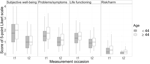
(a)

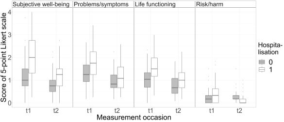
(b)

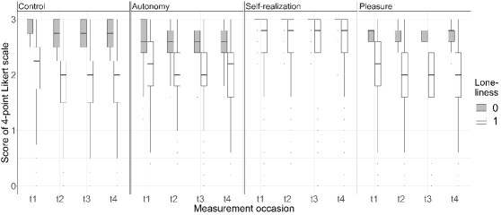
(c)

Figure 1: Boxplots showing the variables’ distribution in the reference datasets:
(a) Dataset 1: CORE-OM dataset, group variable age ($n_{0}=n_{1}=93$)
(b) Dataset 2: CORE-OM dataset, group variable hospitalisation ($n_{0}=42,n_{1}=142$, non-hospitalised patients represent group 0 and hospitalised patients represent group 1)
(c) Dataset 3: CASP-19 dataset, group variable loneliness ($n_{0}=254,n_{1}=1682$, participants who feel less lonely represent group 0 and participants who feel more lonely represent group 1)

2 .5 Simulation study approach and software

Our simulation study aims at mimicking the reference datasets. A brief overview of the steps in the simulation study is given in Figure 2. For each scenario, 2000 datasets are simulated. Data are simulated from the multivariate normal distribution (as a reference), from the multivariate truncated normal distribution which only takes on values within specified boundaries (similar to the scales in the reference data) and multivariate lognormally distributed data in order to include an extremely skewed distribution (overview in Table 3). Data are either not trimmed or trimmed using the MCD and the MVE algorithm, respectively, before applying the classification algorithms.
Sample sizes for the training data are chosen identical to the sample sizes of the original datasets. Sample sizes for the test data are always $n_{0}=n_{1}=1000$ in order to decrease variation of the performance measure estimates.
Application of the linear SVM algorithm requires a data-preprocessing step and finding an optimal hyperparameter $C$ which determines the maximum amount of overlap allowed between samples of both classes. Since the SVM algorithm relies on the Euclidean distance to determine the optimal decision boundary, data are preprocessed by standardization before applying the method. Machine-learning algorithms generally require the optimization of hyperparameters. We applied the simple SVM path (SSVMP) algorithm by Sentelle et al. (2016) as suggested by Chen and Bowman (2011) in order to determine the optimal regularization parameter $C$. It is available as MATLAB code (Sentelle, 2015), which we rewrote in R.
The SSVMP algorithm ran into errors for the largest dataset 3. It did not give results for the vast majority of datasets in scenario 3 (either no convergence was reached after the maximum number of 100 iterations or the assumptions of the Cholesky decomposition originally incorporated in the algorithm were not fulfilled), thus results of the longitudinal SVM are not computed for dataset 3.
The longitudinal SVM algorithm requires to specify a maximum number of iterations used for finding the optimal separating hyperplane parameters. The iterative algorithm for optimization of the Lagrange multipliers $\bm{\alpha}$ and temporal change parameters $\bm{\beta}$ in the longitudinal SVM is repeated until the Euclidean distance between two consecutive estimates of $\bm{\alpha}_{m}$ becomes less than $1\mathrm{E}$−$08$ or the maximum number of 100 iterative steps is reached. The number of times for which the longitudinal SVM algorithm converged in the different settings can be found in Supplementary Table S4.
The MVE and MCD algorithm cannot be applied if the variability in at least one variable is too low to determine unique quantiles. They both failed for the bootstrap approach using dataset 3 (Table 4) because there is hardly any variability for the variable "self-realization" in group 0. The flip-flop algorithm (Lu and Zimmerman, 2005) used by Brobbey (2021) for estimating the Kronecker product structure of the covariance matrix from the training data was iterated until the Frobenius norm of two consecutive Kronecker product covariance matrices became less than or equal to $1\mathrm{E}$−$04$, a proposed stopping criterion by Castaneda and Nossek (2014).
We used the following software for data simulations. We implemented the longitudinal SVM in R and used the R package Rcplex (Bravo et al, 2021), an R interface to linear and quadratic solvers of the IBM ILOG CPLEX Optimization Studio (IBM ILOG, 2021). We used the implementations of MVE and MCD algorithm from the R package MASS (Ripley et al, 2022), the joint GEE model as implemented in the R package JGEE (Inan, 2015), and implemented the version of the flip-flop algorithm in R as described in Lu and Zimmerman (2005). For simulation of multivariate normally, lognormally, truncated normally distributed data, we used the respective functions from the R packages MASS (Ripley et al, 2022), compositions (van den Boogaart et al, 2022), and tmvtnorm (Wilhelm and Manjunath, 2022), respectively. For the truncated normal distribution, the rejection method (default) was used.
We compared the methods’ performance with respect to different measures of discrimination. These consider the similarity between true and predicted class labels. We chose predictive accuracy, the proportion of correctly predicted class labels, and the Youden index (Youden, 1950), which combines the sensitivity and specificity of the classification model in a single measure (Youden index = $|$Sensitivity + Specificity -1$|$). Recommendations based on theses measures can differ a lot. Predictive accuracy of an algorithm may be high in data with highly unbalanced classes if the label of the larger class is predicted for all samples. In this case the Youden index will have the minimum value of zero. Therefore it is reasonable to consider both measures.
For visual assessment, summary ROC curves (Reitsma et al, 2005), which represent sensitivity and specificity estimates for all 2000 simulated datasets in combination, are computed using the R package mada (Doebler, 2020). They are based on a bivariate normal model of sensitivity and specificity, which is identical to the hierarchical summary ROC model by Rutter and Gatsonis (2001) when no covariates affecting either sensitivity or specificity are included (Harbord et al, 2007), and which is recommended for meta-analyses of test performances in the Cochrane Handbook (Cochrane Diagnostic Test Accuracy Working Group, 2011).

Table 3: Parameterizations of the multivariate distributions for group $i\in\{0,1\}$. The multivariate truncated normal distribution is defined by lower and upper boundaries, $\textbf{a}\in\mathds{R}^{pt}$ and $\textbf{b}\in\mathds{R}^{pt}$, respectively, in addition to the mean ($\bm{\mu}_{i}$) and covariance ($\bm{\Sigma}$) parameters.

Distribution	Parameterization
Multivariate normal	$\mathcal{N}_{pt}(\bm{\mu}_{i},\bm{\Sigma})$
Multivariate lognormal	$\mathcal{LN}_{pt}(\bm{\mu}_{i},\bm{\Sigma})$
Multivariate truncated normal	$\mathcal{TN}_{pt}(\bm{\mu}_{i},\bm{\Sigma},\textbf{a},\textbf{b})$

Figure 2: Overview of the steps in the simulation study for a particular reference dataset.

3 Results and discussion

3 .1 Performance in the reference data

Figure 2 shows the ROC curves based on the $\hat{\theta}^{.632+}$ bootstrap estimates of sensitivity and specificity for each reference dataset in order to provide a first visual impression of the algorithms’ performance in the reference data. These estimates of sensitivity and specificity including their 95% confidence intervals can be found in Supplementary Table S2.

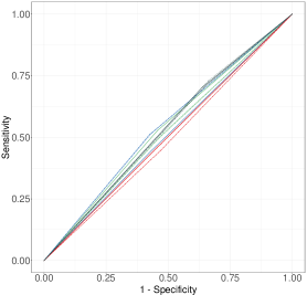
(a)

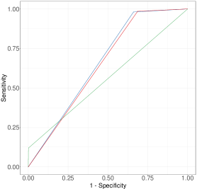
(c)

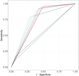
(b)

Figure 2: ROC curves showing the algorithms’ discriminative performance, based on the $\hat{\theta}^{.632+}$ bootstrap estimates of sensitivity and specificity.
(a) Dataset 1: CORE-OM dataset, group variable age ($n_{0}=n_{1}=93$)
(b) Dataset 2: CORE-OM dataset, group variable hospitalisation ($n_{0}=42,n_{1}=142$, non-hospitalised patients represent group 0 and hospitalised patients represent group 1)
(c) Dataset 3: CASP-19 dataset, group variable loneliness ($n_{0}=254,n_{1}=1682$, participants who feel less lonely represent group 0 and participants who feel more lonely represent group 1)

In the balanced scenario (dataset 1), the performance of all methods is very similar and could not distinguish the classes very well. This could already be assumed from the boxplots (Figure 1) which largely overlap for dataset 1. In the unbalanced scenarios (dataset 2 and 3), the different extensions of LDA to repeated measures data clearly perform better than the longitudinal SVM, for which Chen and Bowman (2011) only demonstrated the performance for equal sample sizes. Considering the results, the method may not work as well for highly imbalanced data.
able 4 shows the $\hat{\theta}^{.632+}$ bootstrap estimates for predictive accuracy and the Youden index with their respective 95% confidence intervals. In Dataset 1 (equal sample sizes), the methods’ performance is very similar, and only the longitudinal SVM has a higher predictive accuracy compared to the standard LDA (LDA ($\Sigma_{pooled}$)) with non-overlapping confidence intervals. For the LDA-based methods, performance slightly improves after multivariate outlier removal (application of the MVE or MCD algorithm, respectively). For Dataset 2 (highly imbalanced sample sizes), the most obvious result is the poor performance of the longitudinal SVM. In Dataset 3 (highly imbalanced but larger sample sizes than Dataset 2, less temporal variation), predictive accuracy and Youden Index are much lower for LDA based on GEE estimates compared to the other algorithms.
Results using the MVE and MCD algorithm could not be computed since these methods only work if unique quantiles can be determined but the variable "self-realization" has too low variability in group 0. The results of the longitudinal SVM are missing since the data often did not fulfil the assumptions of the Cholesky decomposition used in the algorithm or the maximum number of 100 iterative steps was exceeded.

Table 4: Performance in the reference data using the bootstrap approach for point estimates by Wahl et al. (2016) and 2000 bootstrap datasets. Mean performance (95% CI) is indicated for each reference dataset. Results with the highest mean are shown in bold. Dataset 1: CORE-OM, group variable age ($n_{0}=n_{1}=93$), Dataset 2: CORE-OM, group variable hospitalisation ($n_{0}=42,n_{1}=142$), Dataset 3: CASP-19, group variable loneliness ($n_{0}=254,n_{1}=1682$).

original					MVE					MCD
LDA ($\Sigma_{pooled}$)	LDA ($\Sigma_{KP}$)	LDA (GEE)	SVM		LDA ($\Sigma_{pooled}$)	LDA ($\Sigma_{KP}$)	LDA (GEE)	SVM		LDA ($\Sigma_{pooled}$)	LDA ($\Sigma_{KP}$)	LDA (GEE)	SVM
Dataset 1
Predictive accuracy
0.461 (0.321, 0.466)	0.519 (0.39, 0.535)	0.514 (0.39, 0.535)	0.54 (0.475, 0.706)		0.485 (0.377, 0.539)	0.54 (0.449, 0.605)	0.52 (0.439, 0.622)	0.536 (0.444, 0.659)		0.497 (0.357, 0.513)	0.536 (0.429, 0.574)	0.52 (0.418, 0.627)	0.539 (0.47, 0.674)
Youden index
0.088 (0, 0.117)	0.099 (0, 0.159)	0.09 (0, 0.134)	0.106 (0, 0.289)		0.104 (0, 0.223)	0.125 (0, 0.266)	0.113 (0, 0.269)	0.099 (0, 0.217)		0.095 (0, 0.149)	0.114 (0, 0.213)	0.104 (0, 0.203)	0.108 (0, 0.269)
Dataset 2
Predictive accuracy
0.844 (0.801, 0.898)	0.84 (0.791, 0.9)	0.765 (0.667, 0.82)	0.296 (0, 0.356)		0.852 (0.814, 0.939)	0.847 (0.803, 0.939)	0.779 (0.724, 0.963)	0.34 (0, 0.394)		0.839 (0.784, 0.92)	0.833 (0.763, 0.91)	0.77 (0.705, 0.95)	0.348 (0, 0.402)
Youden index
0.422 (0.21, 0.646)	0.457 (0.258, 0.63)	0.466 (0.25, 0.575)	0 (0, 0)		0.489 (0.336, 0.756)	0.512 (0.417, 0.821)	0.512 (0.397, 0.873)	0 (0, 0)		0.489 (0.306, 0.716)	0.503 (0.331, 0.715)	0.507 (0.38, 0.872)	0 (0, 0)
Dataset 3
Predictive accuracy
0.897 (0.883, 0.908)	0.896 (0.882, 0.907)	0.236 (0.187, 0.252)
Youden index
0.3 (0.142, 0.412)	0.32 (0.184, 0.448)	0.117 (0.061, 0.133)

3 .2 Performance in the simulated data

Summary ROC plots for all simulation scenarios are shown in Supplementary Figure S1. The summary ROC curves essentially show the better discriminative ability of the classification algorithms in Datasets 2 and 3, respectively, where (mean) measurements between the groups differ more than in Dataset 1.
Complete simulation results showing the mean and standard errors of all performance measures can be found in the supplementary material (Supplementary Table S3). Since the focus is rather comparing the methods’ performance than on the exact numbers, we show a visual comparison of the methods’ predictive accuracy (Figure 3). Since the results with respect to the Youden index are very similar they are shown in Supplementary Figure S2.
Figure 3 shows the boxplots of predictive accuracy estimated in the 2000 test datasets. Notably, the standard repeated measures LDA algorithm (based on the usual pooled covariance estimate, $\bm{\widehat{\Sigma}}_{pooled}$) does not perform best in any simulation scenario, although the difference is especially marginal for Dataset 1. For Dataset 1, the LDA based on the parsimonious Kronecker product covariance ($\Sigma_{KP}$) and LDA based on estimates of the joint GEE model LDA(GEE), respectively, perform slightly better. For Dataset 2 and 3, respectively, LDA(GEE) generally performs best with respect to predictive accuracy (and the Youden index, Supplementary Figure S2), although there are some outliers among the 2000 simulations with worse results. In the nonnormally distributed data (middle and right column), the advantage of multivariate outlier removal through the MVE and MCD algorithms becomes apparent, where the use of the MCD algorithm (in green) often results in higher predictive accuracy compared to the use of the MVE algorithm (in blue). The longitudinal SVM only works comparably well for Dataset 1 (small but balanced sample sizes).
The high computational times for the longitudinal SVM (as a nonparametric method) are another disadvantage (Table 5). The traditional LDA which uses the pooled covariance estimate is least computationally intensive since it does not involve any iterative procedure.

Table 5: Computational times (hours) per algorithm averaged over the simulated datasets per reference dataset (irrespective of the data distribution and irrespective whether trimming has been done before application of the classification algorithm). Dataset 1: CORE-OM, group variable age ($n_{0}=n_{1}=93$), Dataset 2: CORE-OM, group variable hospitalisation ($n_{0}=42,n_{1}=142$), Dataset 3: CASP-19, group variable loneliness ($n_{0}=254,n_{1}=1682$).

	LDA ($\bm{\Sigma}_{pooled}$)	LDA ($\bm{\Sigma}_{KP}$)	LDA (GEE)	SVM
Dataset 1	0.08	1.43	0.62	39.11
Dataset 2	0.08	1.43	0.63	56.43
Dataset 3	0.1	20.46	28.08	−

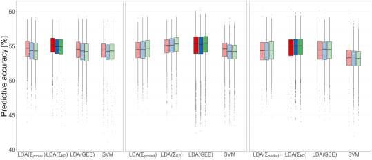
(a)

(b)

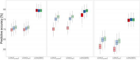
(c)

Figure 3: Boxplots showing the distribution of the algorithms’ predictive accuracy estimated from 2000 simulated datasets for the multivariate normal (left), multivariate lognormal (center) and multivariate truncated normal distribution (right). Results with the highest median value are highlighted in darker colours.
(a) Dataset 1: CORE-OM dataset, group variable age ($n_{0}=n_{1}=93$)
(b) Dataset 2: CORE-OM dataset, group variable hospitalisation ($n_{0}=42,n_{1}=142$)
(c) Dataset 3: CASP-19 dataset, group variable loneliness ($n_{0}=254,n_{1}=1682$)

3 .3 Recommendations

In summary, the (nonparametric) longitudinal SVM seems not to be recommendable due to its poor performance in data with unbalanced class sizes, its relatively high computational times and potential errors the algorithm may run into for some data. However, it may work well for equal class sizes (Chen and Bowman, 2011). Repeated measures LDA based on estimates of the joint GEE model (LDA(GEE)) usually performs best, whether or not the data are normally distributed. Also, results of the LDA(GEE) method are much less affected by multivariate outliers than those of the standard repeated measures LDA (LDA ($\bm{\Sigma}_{pooled}$)) and the LDA using the more parsimonious Kronecker product covariance estimate (LDA ($\bm{\Sigma}_{KP}$)). An additional advantage is also, that the method is already implemented in the R package JGEE (Inan, 2015), and can therefore easily be applied.
LDA ($\bm{\Sigma}_{pooled}$) or LDA ($\bm{\Sigma}_{KP}$) in combination with multivariate outlier removal may still perform better in specific cases. For these classification methods, especially the MCD algorithm for prior outlier removal seems advantageous, that is also implemented in the R package MASS (Ripley et al, 2022).

4 Conclusions

Longitudinal studies are conducted in psychology and other disciplines. Data in psychology and the social sciences are often characterized by nonnormal distributions, especially skewness. LDA is widely applied as a standard technique in these fields, e.g. to questionnaire data where answers are measured on Likert scales, either for classification tasks or for identification of variables most relevant to group separation. Repeated measures techniques are preferable for the analysis of data that are collected repeatedly over time compared to conducting several independent analyses per time point. We compared the performance of robust repeated measures DA techniques proposed by Brobbey et al. (2021; 2022) and the longitudinal SVM by Chen and Bowman (2011) using multiple performance measures. We based these comparisons on real psychometric datasets which differ with respect to sample size, sample size ratio, class overlap, temporal variation and number of repeated measurement occasions. We thus considered additional scenarios to those in Brobbey et al. (2021; 2022), where Kronecker product structures of means and covariances and constant correlations of the variables over time were assumed. We also compared several robust methods among each other in contrast to comparing a particular robust method to the standard method at a time. We included the longitudinal SVM because it is similar to repeated measures LDA in that they are both linear classifiers for which variable weights can additionally be computed and temporal correlations are considered in the analysis. We did not consider extensions of other supervised machine learning algorithms for classification since they usually assume independence between time points (Ribeiro and Freitas, 2019) and do not have a comparably intuitive interpretation of variable weights as the linear SVM. Still they may be useful in case data shall be grouped based on categorical variables, but traditionally scores based on Likert-type data are considered to be continuous variables.
In order to raise awareness of the considered linear classification techniques and their potential application to psychometric data, we compare them in data simulations based on Likert-type data from psychological questionnaires. We computed point estimates of their performance with confidence intervals in the reference data using a nonparametric bootstrap approach and compared their performance in simulated data based on parameter estimates obtained from the reference datasets. We found that the repeated measures LDA based on parameter estimates from the joint GEE model developed by Brobbey et al. (2022) most often gives the best results. The MCD algorithm most often leads to better classification performance when the (original) data show some group mean difference (only partially or non-overlapping boxes in boxplots). Both methods have already been implemented. The results of one of the methods or both methods in combination can be computed at least as an additional sensitivity analysis.
Potential drawbacks of our study are the limited number of reference datasets considered for the method comparison and the single trimming parameter value (10%) for outlier removal used for the MVE and MCD algorithm. To date, no recommendations on the choice of the trimming parameter for multivariate data exist. Multiple values can be tried for the analysis of an actual dataset.
We followed the guidelines for neutral comparison studies by Weber et al. (2019) and the general design of simulation studies by Morris et al. (2019).

Supplementary information

R .1 Longitudinal Support Vector Machine

SVM is based on the structural risk minimization (SRM) principle which is intended to minimize the expectation of the test error for a trained SVM model, called the expected risk $R(a)$. Its value usually cannot be computed directly but the upper boundary is given by the sum of the mean error $R_{emp}(a)$ and the so-called Vapnik-Chervonenkis confidence. Among a predefined set of functions, as, for example, the set of linear functions, the one which yields the maximum margin between the samples of both classes is determined.
The upper bound of the expected risk $R(a)$ holds with a probability of $1-\eta$ and is defined as (Vapnik, 2010; Burges, 1998):

$$R(a) \leq R_{emp}(a)+\sqrt{\left(\frac{h(\log(2n/h)+1)-\log(\eta/4)}{n}\right)}\quad,\text{ where}$$

$$R_{emp}(a) =\frac{1}{2}\sum\limits_{i=1}^{n}|y_{j}-f(\textbf{x}_{j},a)|$$

and $n$ denotes the number of training observations, $a$ a specific support vector machine model, $h$ the Vapnik-Chervonenkis dimension (which equals $n+1$ for the linear SVM), and $f(\textbf{x}_{j},a)$ representing the predicted class labels by model $a$.
The SSVMP algorithm (Sentelle, 2015; Sentelle et al, 2016) optimizes the inverse of the regularization parameter, $\lambda=1/C$. Starting with a high value of $\lambda$ such that all samples lie within the margin of the SVM, it successively determines a strictly decreasing sequence of $\lambda$ values for which the set of support vectors changes for each $\lambda$ value, and it stops if no more observations are left inside of the margin (linearly separable case) or if the next $\lambda$ value would be zero.
In the algorithm by Chen and Bowman (2011), the linear kernel matrix (or Gram matrix) $\textbf{G}_{m}$ is given by:

$$\textbf{G}_{m} =\begin{pmatrix}\textbf{G}_{m}^{11}&\dots&\textbf{G}_{m}^{1t}\\ \vdots&\ddots&\vdots\\ \textbf{G}_{m}^{t1}&\dots&\textbf{G}_{m}^{tt}\end{pmatrix}=\begin{pmatrix}\textbf{X}_{1}^{T}\textbf{X}_{1}&\dots&\textbf{X}_{1}^{T}\textbf{X}_{t}\\ \vdots&\ddots&\vdots\\ \textbf{X}_{t}^{T}\textbf{X}_{1}&\dots&\textbf{X}_{t}^{T}\textbf{X}_{t}\end{pmatrix}\in\mathds{R}^{nt\times nt}$$

 where

$$\textbf{X}_{k} =\begin{pmatrix}y_{1}\textbf{x}_{1k}\\ \vdots\\ y_{n}\textbf{x}_{nk}\end{pmatrix}\in\mathds{R}^{n\times p},\quad k=1,\dots,t.$$

The dual form of the convex quadratic program (QP) is given by:

$$\hskip 14.22636pt\min\limits_{\bm{\alpha}}\frac{1}{2}\bm{\alpha}_{m}^{T}\textbf{G}_{m}\bm{\alpha}_{m}-\textbf{1}^{T}\bm{\alpha}$$

s.t. $$\hskip 14.22636ptC\geq\alpha_{j}\geq 0\quad\forall j=1,\dots,n\hskip 35.56593pt\sum\limits_{k=1}^{t}\sum\limits_{j=1}^{n}\bm{\alpha}_{m}(j+(k-1)n)y_{j}=0$$

where

$$\hskip 14.22636pt\bm{\alpha}_{m}=(\bm{\alpha},\beta_{1}\bm{\alpha},\dots,\beta_{t-1}\bm{\alpha})^{T}\in\mathds{R}^{tn\times 1}$$

and $\bm{\alpha}_{m}^{T}\textbf{G}_{m}\bm{\alpha}_{m}$ is a convex function in the Lagrange multipliers $\bm{\alpha}$ and the temporal change parameters $\bm{\beta}$. The parameters $\bm{\alpha}$ and $\bm{\beta}$ can be optimized iteratively with respect to this objective function:

1. [1.]

2. Initialize $\bm{\beta}=(1,\beta_{1},\dots,\beta_{t-1})$.

3. Assuming the value of $\bm{\beta}$ is known, $\bm{\alpha}$ is optimized. The optimization problem becomes:

   $$\hskip 14.22636pt\min\limits_{\bm{\alpha}}\frac{1}{2}\bm{\alpha}^{T}\left(\sum\limits_{k_{1}=1}^{t}\sum\limits_{k_{2}=1}^{t}\beta_{k_{1}}\beta_{k_{2}}\textbf{G}_{m}^{k_{1}k_{2}}\right)\bm{\alpha}-\textbf{1}^{T}\bm{\alpha}$$

   s.t. $$\hskip 14.22636ptC\geq\alpha_{j}\geq 0\quad\forall j=1,\dots,n\hskip 35.56593pt\sum\limits_{j=1}^{n}\alpha_{j}y_{j}=0$$

4. Assuming the value of $\bm{\alpha}$ is known, $\bm{\beta}$ is optimized. The optimization problem becomes:

   $$\hskip 14.22636pt\min\limits_{\bm{\beta}}\frac{1}{2}\bm{\beta}^{T}\begin{pmatrix}\bm{\alpha}^{T}\textbf{G}_{m}^{11}\bm{\alpha}&\dots&\bm{\alpha}^{T}\textbf{G}_{m}^{1t}\bm{\alpha}\\ \vdots&\ddots&\vdots\\ \bm{\alpha}^{T}\textbf{G}_{m}^{t1}\bm{\alpha}&\dots&\bm{\alpha}^{T}\textbf{G}_{m}^{tt}\bm{\alpha}\end{pmatrix}\bm{\beta}$$

   s.t. $$\hskip 14.22636pt\beta_{0}=1\hskip 35.56593pt\left(\sum\limits_{j=1}^{n}\alpha_{j}y_{j}\right)\sum\limits_{k=1}^{t}\beta_{k}=0$$

Steps 2 and 3 are repeated until convergence.
The dual form allows to directly identify the support vectors. Their corresponding entries of $\bm{\alpha}_{m}$ are different from zero, i.e. $\textbf{x}_{j}$ is a support vector if $\left\{\bm{\alpha}_{m}(j+(k-1)n)\right\}_{k=1,\dots,t}>\textbf{0}\quad j\in\{1,\dots,n\}$.
Having found the optimal solution $\bm{\alpha}_{m}^{*}$ through the iterative QP approach, the weight vector w and the intercept $b$ in the decision function $h$ can be determined:

$$h(\textbf{x}) =\frac{1}{n}\sum\limits_{j=1}^{n}\textbf{w}^{T}\textbf{x}^{T}\bm{\beta}^{*}+b$$

where

w $$=\sum\limits_{j=1}^{n}y_{j}\alpha_{j}^{*}\widetilde{\textbf{x}}_{j}=\sum\limits_{j=1}^{n}y_{j}\alpha_{j}^{*}\{\textbf{x}_{j1}+\beta_{1}^{*}\textbf{x}_{j2}+...+\beta_{t-1}^{*}\textbf{x}_{jt}\}\quad\in\mathds{R}^{p}$$

$$b =\frac{1}{n}\sum\limits_{j=1}^{n}\textbf{w}^{T}(\textbf{x}_{j}^{T}\bm{\beta}^{*})-y_{j}\quad\in\mathds{R}$$

For computation of the intercept $b$, the data $\textbf{x}_{j}$ are used in $t\times p$ matrix form. New data samples are assigned negative class labels ($y=-1$) if $h(\textbf{x})<1$, otherwise they are assigned to the positive class ($y=1$).

Table S 1a: Parameters estimated from Dataset 1: CORE-OM dataset, group variable age (variable 1: subjective well-being, variable 2: problems/symptoms, variable 3: life functioning, variable 4: risk/harm).

Parameter	Description	Estimate
$n_{0}$	sample size group 0	93
$n_{1}$	sample size group 1	93
$n_{test}$	test sample sizes	$n_{0}=n_{1}=1000$
$n_{sim}$	simulation runs	2000
$\bm{\mu}_{0}$	class mean group 0	$\begin{pmatrix}1.75,&1.58,&1.36,&0.32,&1.05,&1.03,&0.91,&0.16\end{pmatrix}^{T}$
$\bm{\mu}_{1}$	class mean group 1	$\begin{pmatrix}1.93,&1.82,&1.53,&0.42,&1.15,&1.19,&1.04,&0.2\end{pmatrix}^{T}$
$\bm{\Sigma}$	pooled covariance matrix	${\scriptsize\begin{pmatrix}0.85&0.41&0.34&0.15&0.40&0.26&0.23&0.03\\ 0.41&0.53&0.26&0.14&0.20&0.36&0.20&0.06\\ 0.34&0.26&0.36&0.11&0.16&0.18&0.23&0.02\\ 0.15&0.14&0.11&0.16&0.08&0.11&0.09&0.06\\ 0.40&0.20&0.16&0.08&0.34&0.16&0.14&0.03\\ 0.26&0.36&0.18&0.11&0.16&0.30&0.16&0.05\\ 0.23&0.20&0.23&0.09&0.14&0.16&0.22&0.03\\ 0.03&0.06&0.02&0.06&0.03&0.05&0.03&0.06\\ \end{pmatrix}}$
$\bm{\Sigma}_{t\times t}$	correlation matrix (time points)	${\scriptsize\begin{pmatrix}1&0.82\\ 0.82&1\end{pmatrix}}$
$\bm{\Sigma}_{p\times p}$	correlation matrix (variables)	${\scriptsize\begin{pmatrix}1&0.42&0.44&0.27\\ 0.42&1&0.5&0.22\\ 0.44&0.5&1&0.2\\ 0.27&0.22&0.2&1\end{pmatrix}}$

Table S 1b: Parameters estimated from Dataset 2: CORE-OM dataset, group variable hospitalisation (variable 1: subjective well-being, variable 2: problems/symptoms, variable 3: life functioning, variable 4: risk/harm).

Parameter	Description	Estimate
$n_{0}$	sample size group 0	42
$n_{1}$	sample size group 1	142
$n_{test}$	test sample sizes	$n_{0}=n_{1}=1000$
$n_{sim}$	simulation runs	2000
$\bm{\mu}_{0}$	class mean group 0	$\begin{pmatrix}1.16,&1.31,&1.06,&0.26,&0.88,&0.92,&0.79,&0.27\end{pmatrix}^{T}$
$\bm{\mu}_{1}$	class mean group 1	$\begin{pmatrix}2.04,&1.81,&1.55,&0.4,&1.16,&1.16,&1.03,&0.15\end{pmatrix}^{T}$
$\bm{\Sigma}$	pooled covariance matrix	$\scriptsize{\begin{pmatrix}0.73&0.34&0.28&0.13&0.37&0.24&0.2&0.05\\ 0.34&0.51&0.22&0.14&0.18&0.35&0.18&0.07\\ 0.28&0.22&0.33&0.1&0.14&0.17&0.22&0.04\\ 0.13&0.14&0.1&0.16&0.07&0.11&0.09&0.07\\ 0.37&0.18&0.14&0.07&0.34&0.15&0.13&0.04\\ 0.24&0.35&0.17&0.11&0.15&0.3&0.16&0.06\\ 0.2&0.18&0.22&0.09&0.13&0.16&0.22&0.04\\ 0.05&0.07&0.04&0.07&0.04&0.06&0.04&0.06\\ \end{pmatrix}}$
$\bm{\Sigma}_{t\times t}$	correlation matrix (time points)	$\scriptsize{\begin{pmatrix}1&0.82\\ 0.82&1\end{pmatrix}}$
$\bm{\Sigma}_{p\times p}$	correlation matrix (variables)	$\scriptsize{\begin{pmatrix}1&0.4&0.43&0.24\\ 0.4&1&0.47&0.21\\ 0.43&0.47&1&0.2\\ 0.24&0.21&0.2&1\end{pmatrix}}$

Table S 1c: Parameters estimated from Dataset 2: CASP-19 dataset, group variable loneliness (variable 1: control, variable 2: autonomy, variable 3: self-realization, variable 4: pleasure).

Parameter	Description	Estimate
$n_{0}$	sample size group 0	254
$n_{1}$	sample size group 1	1682
$n_{test}$	test sample sizes	$n_{0}=n_{1}=1000$
$n_{sim}$	simulation runs	2000
$\bm{\mu}_{0}$	class mean group 0	(2.84, 2.59, 2.96, 2.75, 2.71, 2.58, 2.96, 2.70, 2.67, 2.61, 2.96, 2.70, 2.67, 2.62, 2.95, 2.68 )T
$\bm{\mu}_{1}$	class mean group 1	(2.09, 2.13, 2.67, 2.06, 1.88, 2.07, 2.63, 2.0, 1.86, 2.07, 2.62, 1.96, 1.85, 2.06, 2.61, 1.94)T
$\bm{\Sigma}$	pooled covariance matrix	$\tiny{\setcounter{MaxMatrixCols}{16}\begin{pmatrix}0.31&0.15&0.1&0.18&0.19&0.12&0.1&0.16&0.18&0.12&0.09&0.15&0.18&0.13&0.1&0.16\\ 0.15&0.25&0.08&0.13&0.11&0.15&0.06&0.11&0.11&0.14&0.06&0.1&0.11&0.14&0.07&0.10\\ 0.1&0.08&0.18&0.16&0.08&0.06&0.11&0.11&0.07&0.06&0.11&0.11&0.08&0.06&0.11&0.11\\ 0.18&0.13&0.16&0.32&0.15&0.11&0.13&0.22&0.14&0.11&0.13&0.22&0.16&0.12&0.14&0.22\\ 0.19&0.11&0.08&0.15&0.31&0.16&0.11&0.19&0.21&0.14&0.09&0.17&0.2&0.14&0.1&0.17\\ 0.12&0.15&0.06&0.11&0.16&0.25&0.08&0.14&0.13&0.17&0.07&0.12&0.13&0.16&0.07&0.12\\ 0.1&0.06&0.11&0.13&0.11&0.08&0.17&0.16&0.1&0.07&0.12&0.13&0.1&0.07&0.12&0.13\\ 0.16&0.11&0.11&0.22&0.19&0.14&0.16&0.31&0.17&0.12&0.13&0.23&0.17&0.12&0.14&0.24\\ 0.18&0.11&0.07&0.14&0.21&0.13&0.1&0.17&0.31&0.16&0.1&0.19&0.22&0.14&0.11&0.18\\ 0.12&0.14&0.06&0.11&0.14&0.17&0.07&0.12&0.16&0.24&0.08&0.14&0.14&0.17&0.08&0.13\\ 0.09&0.06&0.11&0.13&0.09&0.07&0.12&0.13&0.1&0.08&0.19&0.16&0.1&0.07&0.13&0.14\\ 0.15&0.1&0.11&0.22&0.17&0.12&0.13&0.23&0.19&0.14&0.16&0.33&0.19&0.13&0.15&0.26\\ 0.18&0.11&0.08&0.16&0.2&0.13&0.1&0.17&0.22&0.14&0.1&0.19&0.34&0.18&0.13&0.22\\ 0.13&0.14&0.06&0.12&0.14&0.16&0.07&0.12&0.14&0.17&0.07&0.13&0.18&0.26&0.09&0.16\\ 0.1&0.07&0.11&0.14&0.1&0.07&0.12&0.14&0.11&0.08&0.13&0.15&0.13&0.09&0.19&0.18\\ 0.16&0.1&0.11&0.22&0.17&0.12&0.13&0.24&0.18&0.13&0.14&0.26&0.22&0.16&0.18&0.36\end{pmatrix}}$
$\bm{\Sigma}_{t\times t}$	correlation matrix (time points)	$\scriptsize{\begin{pmatrix}1&0.69&0.66&0.64\\ 0.69&1&0.75&0.73\\ 0.66&0.75&1&0.76\\ 0.64&0.73&0.76&1\end{pmatrix}}$
$\bm{\Sigma}_{p\times p}$	correlation matrix (variables)	$\scriptsize{\begin{pmatrix}1&0.39&0.27&0.37\\ 0.39&1&0.22&0.31\\ 0.27&0.22&1&0.51\\ 0.37&0.31&0.51&1\end{pmatrix}}$

Table S 2: Performance in the reference data using the bootstrap approach by Wahl et al. (2016) and 2000 bootstrap datasets. Mean performance (95% confidence interval) is indicated for each reference dataset, i.e. Dataset 1: CORE-OM, group variable age ($n_{0}=n_{1}=93$), Dataset 2: CORE-OM, group variable hospitalisation ($n_{0}=42,n_{1}=142$), Dataset 3: CASP-19, group variable loneliness ($n_{0}=254,n_{1}=1682$). The highest point estimates $\hat{\theta}^{.632+}$ are shown in bold.
MVE: Minimum volume ellipsoid, MCD: Minimum covariance determinant, LDA: Linear discriminant analysis, SVM: Support vector machine, $\Sigma_{pooled}$: pooled covariance matrix, $\Sigma_{KP}$: Kronecker product covariance matrix, GEE: covariance matrix of Generalized estimating equation.

original					MVE					MCD
LDA ($\Sigma_{pooled}$)	LDA ($\Sigma_{KP}$)	LDA (GEE)	SVM		LDA ($\Sigma_{pooled}$)	LDA ($\Sigma_{KP}$)	LDA (GEE)	SVM		LDA ($\Sigma_{pooled}$)	LDA ($\Sigma_{KP}$)	LDA (GEE)	SVM
Dataset 1
Predictive accuracy
0.461 (0.321, 0.466)	0.519 (0.39, 0.535)	0.514 (0.39, 0.535)	0.54 (0.475, 0.706)		0.485 (0.377, 0.539)	0.54 (0.449, 0.605)	0.52 (0.439, 0.622)	0.536 (0.444, 0.659)		0.497 (0.357, 0.513)	0.536 (0.429, 0.574)	0.52 (0.418, 0.627)	0.539 (0.47, 0.674)
Youden index
0.088 (0, 0.117)	0.099 (0, 0.159)	0.09 (0, 0.134)	0.106 (0, 0.289)		0.104 (0, 0.223)	0.125 (0, 0.266)	0.113 (0, 0.269)	0.099 (0, 0.217)		0.095 (0, 0.149)	0.114 (0, 0.213)	0.104 (0, 0.203)	0.108 (0, 0.269)
Sensitivity
0.461 (0.134, 0.601)	0.444 (0.212, 0.641)	0.527 (0.359, 0.564)	0.702 (0.594, 1)		0.445 (0.275, 0.663)	0.511 (0.342, 0.703)	0.498 (0.405, 0.633)	0.706 (0.613, 1)		0.473 (0.254, 0.619)	0.516 (0.302, 0.642)	0.517 (0.405, 0.659)	0.729 (0.679, 1)
Specificity
0.543 (0.337, 0.784)	0.569 (0.343, 0.746)	0.543 (0.406, 0.623)	0.363 (0, 0.653)		0.532 (0.316, 0.697)	0.575 (0.424, 0.756)	0.535 (0.411, 0.654)	0.353 (0, 0.472)		0.528 (0.318, 0.673)	0.567 (0.427, 0.741)	0.519 (0.378, 0.622)	0.339 (0, 0.427)
Dataset 2
Predictive accuracy
0.844 (0.801, 0.898)	0.84 (0.791, 0.9)	0.765 (0.667, 0.82)	0.296 (0, 0.357)		0.852 (0.814, 0.939)	0.847 (0.803, 0.939)	0.779 (0.724, 0.963)	0.34 (0, 0.394)		0.839 (0.784, 0.92)	0.833 (0.763, 0.91)	0.77 (0.705, 0.95)	0.348 (0, 0.402)
Youden index
0.422 (0.21, 0.646)	0.457 (0.258, 0.63)	0.466 (0.25, 0.575)	0 (0, 0)		0.489 (0.336, 0.756)	0.512 (0.417, 0.821)	0.502 (0.397, 0.873)	0 (0, 0)		0.489 (0.306, 0.716)	0.503 (0.331, 0.715)	0.507 (0.38, 0.872)	0 (0, 0)
Sensitivity
0.958 (0.937, 1)	0.937 (0.895, 1)	0.792 (0.685, 0.865)	0.095 (0, 0.095)		0.944 (0.902, 1)	0.921 (0.836, 1)	0.802 (0.717, 1)	0.158 (0, 0.158)		0.919 (0.862, 1)	0.901 (0.809, 0.999)	0.783 (0.679, 0.966)	0.167 (0, 0.167)
Specificity
0.5 (0.264, 0.727)	0.52 (0.289, 0.71)	0.673 (0.499, 0.788)	0.957 (0.957, 1)		0.54 (0.361, 0.806)	0.571 (0.467, 0.928)	0.697 (0.571, 0.98)	0.941 (0.941, 1)		0.57 (0.363, 0.793)	0.6 (0.431, 0.861)	0.721 (0.602, 1)	0.939 (0.939, 1)

Table S 2 (continued): Performance in the reference data using the bootstrap approach by Wahl et al. (2016) and 2000 bootstrap datasets. Mean performance (95% confidence interval) is indicated for each reference dataset, i.e. Dataset 1: CORE-OM, group variable age ($n_{0}=n_{1}=93$), Dataset 2: CORE-OM, group variable hospitalisation ($n_{0}=42,n_{1}=142$), Dataset 3: CASP-19, group variable loneliness ($n_{0}=254,n_{1}=1682$). The highest point estimates $\hat{\theta}^{.632+}$ are shown in bold.
MVE: Minimum volume ellipsoid, MCD: Minimum covariance determinant, LDA: Linear discriminant analysis, SVM: Support vector machine, $\Sigma_{pooled}$: pooled covariance matrix, $\Sigma_{KP}$: Kronecker product covariance matrix, GEE: covariance matrix of Generalized estimating equation.

original					MVE					MCD
LDA ($\Sigma_{pooled}$)	LDA ($\Sigma_{KP}$)	LDA (GEE)	SVM		LDA ($\Sigma_{pooled}$)	LDA ($\Sigma_{KP}$)	LDA (GEE)	SVM		LDA ($\Sigma_{pooled}$)	LDA ($\Sigma_{KP}$)	LDA (GEE)	SVM
Dataset 1
Predictive accuracy
0.897 (0.883, 0.908)	0.896 (0.992, 0.907)	0.236 (0.187, 0.252)
Youden index
0.3 (0.142, 0.412)	0.32 (0.184, 0.448)	0.117 (0.061, 0.133)
Sensitivity
0.985 (0.981, 0.999)	0.981 (0.971, 0.994)	0.12 (0.062, 0.133)
Specificity
0.314 (0.145, 0.426)	0.34 (0.193, 0.472)	0.999 (0.999, 1)

Table S 3a: Performance of the algorithms in 2000 simulated datasets for dataset 1 (CORE-OM dataset, group variable age, training data: $n_{0}=n_{1}=93$, test data: $n_{0}=n_{1}=1000$). Data are simulated from the multivariate normally ($\mathcal{N}$), lognormally ($\mathcal{LN}$) and truncated normally ($\mathcal{TN}$) distribution. Parameter estimates are obtained from the training data without trimming (original) or after trimming by applying the MVE or MCD algorithm, respectively, keeping 90% of the training data. Highest mean values are shown in bold.
MVE: Minimum volume ellipsoid, MCD: Minimum covariance determinant, LDA: Linear discriminant analysis, SVM: Support vector machine, $\Sigma_{pooled}$: pooled covariance matrix, $\Sigma_{KP}$: Kronecker product covariance matrix, GEE: covariance matrix of Generalized estimating equation.

	original					MVE					MCD
	LDA ($\Sigma_{pooled}$)	LDA ($\Sigma_{KP}$)	LDA (GEE)	SVM		LDA ($\Sigma_{pooled}$)	LDA ($\Sigma_{KP}$)	LDA (GEE)	SVM		LDA ($\Sigma_{pooled}$)	LDA ($\Sigma_{KP}$)	LDA (GEE)	SVM
Predictive accuracy
$\mathcal{N}$	0.545 (0.018)	0.55 (0.017)	0.544 (0.019)	0.541 (0.021)		0.542 (0.019)	0.547 (0.018)	0.54 (0.02)	0.538 (0.023)		0.541 (0.019)	0.547 (0.019)	0.539 (0.021)	0.539 (0.023)
$\mathcal{LN}$	0.543 (0.018)	0.548 (0.019)	0.546 (0.029)	0.542 (0.021)		0.543 (0.019)	0.549 (0.02)	0.546 (0.027)	0.539 (0.022)		0.545 (0.018)	0.55 (0.018)	0.55 (0.023)	0.539 (0.02)
$\mathcal{TN}$	0.542 (0.02)	0.546 (0.021)	0.542 (0.021)	0.532 (0.021)		0.542 (0.02)	0.547 (0.021)	0.542 (0.021)	0.531 (0.021)		0.543 (0.02)	0.547 (0.021)	0.543 (0.021)	0.531 (0.02)
Youden index
$\mathcal{N}$	0.091 (0.033)	0.101 (0.031)	0.088 (0.034)	0.087 (0.031)		0.085 (0.034)	0.096 (0.032)	0.083 (0.035)	0.083 (0.033)		0.084 (0.035)	0.095 (0.034)	0.082 (0.035)	0.084 (0.033)
$\mathcal{LN}$	0.087 (0.033)	0.098 (0.031)	0.101 (0.038)	0.089 (0.031)		0.088 (0.035)	0.099 (0.033)	0.1 (0.038)	0.084 (0.032)		0.091 (0.035)	0.102 (0.033)	0.103 (0.036)	0.083 (0.031)
$\mathcal{TN}$	0.085 (0.037)	0.094 (0.037)	0.086 (0.037)	0.069 (0.032)		0.085 (0.037)	0.096 (0.036)	0.086 (0.037)	0.066 (0.031)		0.087 (0.037)	0.097 (0.036)	0.087 (0.037)	0.066 (0.03)
Sensitivity
$\mathcal{N}$	0.546 (0.035)	0.55 (0.034)	0.544 (0.035)	0.7 (0.145)		0.543 (0.038)	0.548 (0.038)	0.541 (0.039)	0.689 (0.148)		0.542 (0.039)	0.547 (0.039)	0.54 (0.04)	0.688 (0.148)
$\mathcal{LN}$	0.469 (0.04)	0.468 (0.04)	0.479 (0.04)	0.647 (0.177)		0.512 (0.041)	0.52 (0.04)	0.521 (0.045)	0.668 (0.174)		0.52 (0.042)	0.531 (0.041)	0.529 (0.044)	0.676 (0.178)
$\mathcal{TN}$	0.515 (0.046)	0.512 (0.046)	0.512 (0.045)	0.714 (0.195)		0.536 (0.043)	0.537 (0.043)	0.534 (0.043)	0.725 (0.198)		0.542 (0.043)	0.544 (0.043)	0.54 (0.043)	0.733 (0.192)
Specificity
$\mathcal{N}$	0.544 (0.035)	0.549 (0.035)	0.543 (0.036)	0.383 (0.139)		0.541 (0.039)	0.547 (0.038)	0.54 (0.04)	0.388 (0.14)		0.54 (0.04)	0.546 (0.039)	0.539 (0.041)	0.389 (0.138)
$\mathcal{LN}$	0.617 (0.051)	0.628 (0.054)	0.612 (0.063)	0.438 (0.172)		0.574 (0.044)	0.578 (0.044)	0.571 (0.048)	0.411 (0.17)		0.57 (0.043)	0.57 (0.042)	0.57 (0.044)	0.402 (0.174)
$\mathcal{TN}$	0.569 (0.05)	0.58 (0.053)	0.573 (0.052)	0.349 (0.192)		0.548 (0.043)	0.557 (0.044)	0.55 (0.044)	0.336 (0.195)		0.544 (0.041)	0.551 (0.042)	0.545 (0.042)	0.328 (0.189)

Table S 3b: Performance of the algorithms in 2000 simulated datasets for dataset 2 (CORE-OM dataset, group variable hospitalisation, training data: $n_{0}=42,n_{1}=142$, test data: $n_{0}=n_{1}=1000$). Data are simulated from the multivariate normally ($\mathcal{N}$), lognormally ($\mathcal{LN}$) and truncated normally ($\mathcal{TN}$) distribution. Parameter estimates are obtained from the training data without trimming (original) or after trimming by applying the MVE or MCD algorithm, respectively, keeping 90% of the training data. Highest mean values are shown in bold.
MVE: Minimum volume ellipsoid, MCD: Minimum covariance determinant, LDA: Linear discriminant analysis, SVM: Support vector machine, $\Sigma_{pooled}$: pooled covariance matrix, $\Sigma_{KP}$: Kronecker product covariance matrix, GEE: covariance matrix of Generalized estimating equation.

	original					MVE					MCD
	LDA ($\Sigma_{pooled}$)	LDA ($\Sigma_{KP}$)	LDA (GEE)	SVM		LDA ($\Sigma_{pooled}$)	LDA ($\Sigma_{KP}$)	LDA (GEE)	SVM		LDA ($\Sigma_{pooled}$)	LDA ($\Sigma_{KP}$)	LDA (GEE)	SVM
Predictive accuracy
$\mathcal{N}$	0.712 (0.019)	0.71 (0.015)	0.735 (0.022)	0.559 (0.078)		0.716 (0.021)	0.713 (0.016)	0.73 (0.03)	0.572 (0.08)		0.719 (0.021)	0.715 (0.016)	0.729 (0.03)	0.58 (0.081)
$\mathcal{LN}$	0.647 (0.025)	0.646 (0.028)	0.703 (0.051)	0.516 (0.051)		0.668 (0.025)	0.666 (0.025)	0.712 (0.048)	0.541 (0.076)		0.673 (0.024)	0.67 (0.023)	0.719 (0.042)	0.557 (0.084)
$\mathcal{TN}$	0.671 (0.034)	0.682 (0.032)	0.757 (0.015)	0.542 (0.071)		0.707 (0.028)	0.715 (0.023)	0.755 (0.018)	0.575 (0.079)		0.713 (0.026)	0.723 (0.02)	0.755 (0.017)	0.578 (0.079)
Youden index
$\mathcal{N}$	0.425 (0.039)	0.42 (0.03)	0.471 (0.044)	0.117 (0.156)		0.433 (0.042)	0.426 (0.033)	0.461 (0.053)	0.144 (0.16)		0.438 (0.041)	0.43 (0.033)	0.459 (0.056)	0.159 (0.162)
$\mathcal{LN}$	0.295 (0.049)	0.292 (0.055)	0.407 (0.099)	0.031 (0.101)		0.335 (0.051)	0.331 (0.049)	0.425 (0.094)	0.082 (0.152)		0.345 (0.048)	0.339 (0.046)	0.439 (0.082)	0.113 (0.168)
$\mathcal{TN}$	0.343 (0.069)	0.363 (0.065)	0.514 (0.03)	0.084 (0.142)		0.414 (0.057)	0.43 (0.046)	0.51 (0.035)	0.144 (0.159)		0.427 (0.052)	0.445 (0.04)	0.511 (0.033)	0.156 (0.157)
Sensitivity
$\mathcal{N}$	0.93 (0.017)	0.903 (0.022)	0.746 (0.034)	0.185 (0.256)		0.919 (0.021)	0.895 (0.025)	0.743 (0.039)	0.237 (0.271)		0.915 (0.021)	0.892 (0.025)	0.743 (0.042)	0.259 (0.273)
$\mathcal{LN}$	0.945 (0.019)	0.928 (0.028)	0.661 (0.067)	0.05 (0.167)		0.938 (0.021)	0.923 (0.026)	0.709 (0.065)	0.139 (0.267)		0.942 (0.019)	0.927 (0.024)	0.726 (0.056)	0.195 (0.299)
$\mathcal{TN}$	0.929 (0.018)	0.93 (0.019)	0.768 (0.033)	0.139 (0.245)		0.901 (0.022)	0.905 (0.02)	0.769 (0.033)	0.243 (0.279)		0.896 (0.021)	0.898 (0.019)	0.767 (0.032)	0.265 (0.28)
Specificity
$\mathcal{N}$	0.495 (0.05)	0.517 (0.041)	0.725 (0.039)	0.932 (0.107)		0.514 (0.056)	0.531 (0.045)	0.718 (0.046)	0.912 (0.115)		0.523 (0.054)	0.538 (0.045)	0.716 (0.047)	0.901 (0.119)
$\mathcal{LN}$	0.35 (0.063)	0.364 (0.077)	0.745 (0.068)	0.981 (0.069)		0.396 (0.064)	0.408 (0.068)	0.716 (0.058)	0.942 (0.119)		0.404 (0.061)	0.412 (0.063)	0.713 (0.054)	0.919 (0.137)
$\mathcal{TN}$	0.413 (0.082)	0.433 (0.079)	0.746 (0.033)	0.944 (0.107)		0.513 (0.069)	0.526 (0.059)	0.741 (0.037)	0.901 (0.129)		0.531 (0.064)	0.547 (0.051)	0.743 (0.035)	0.892 (0.134)

Table S 3c: Performance of the algorithms in 2000 simulated datasets for dataset 3 (CASP-19 dataset, group variable loneliness, training data: $n_{0}=254,n_{1}=1682$, test data: $n_{0}=n_{1}=1000$). Data are simulated from the multivariate normally ($\mathcal{N}$), lognormally ($\mathcal{LN}$) and truncated normally ($\mathcal{TN}$) distribution. Parameter estimates are obtained from the training data without trimming (original) or after trimming by applying the MVE or MCD algorithm, respectively, keeping 90% of the training data. Highest mean values are shown in bold.
MVE: Minimum volume ellipsoid, MCD: Minimum covariance determinant, LDA: Linear discriminant analysis, SVM: Support vector machine, $\Sigma_{pooled}$: pooled covariance matrix, $\Sigma_{KP}$: Kronecker product covariance matrix, GEE: covariance matrix of Generalized estimating equation.

	original				MVE				MCD
	LDA ($\Sigma_{pooled}$)	LDA ($\Sigma_{KP}$)	LDA (GEE)		LDA ($\Sigma_{pooled}$)	LDA ($\Sigma_{KP}$)	LDA (GEE)		LDA ($\Sigma_{pooled}$)	LDA ($\Sigma_{KP}$)	LDA (GEE)
Predictive accuracy
$\mathcal{N}$	0.698 (0.011)	0.698 (0.011)	0.795 (0.01)		0.705 (0.013)	0.705 (0.012)	0.794 (0.01)		0.711 (0.011)	0.71 (0.011)	0.794 (0.01)
$\mathcal{LN}$	0.701 (0.011)	0.707 (0.011)	0.772 (0.013)		0.751 (0.011)	0.753 (0.01)	0.789 (0.011)		0.763 (0.01)	0.764 (0.01)	0.794 (0.01)
$\mathcal{TN}$	0.614 (0.018)	0.596 (0.02)	0.745 (0.011)		0.647 (0.016)	0.633 (0.017)	0.749 (0.011)		0.652 (0.015)	0.642 (0.016)	0.748 (0.011)
Youden index
$\mathcal{N}$	0.395 (0.022)	0.397 (0.021)	0.59 (0.02)		0.41 (0.025)	0.409 (0.023)	0.587 (0.021)		0.421 (0.023)	0.42 (0.022)	0.589 (0.02)
$\mathcal{LN}$	0.403 (0.023)	0.414 (0.022)	0.543 (0.026)		0.502 (0.022)	0.507 (0.021)	0.579 (0.021)		0.526 (0.021)	0.529 (0.02)	0.588 (0.02)
$\mathcal{TN}$	0.227 (0.036)	0.191 (0.04)	0.491 (0.022)		0.295 (0.033)	0.266 (0.034)	0.498 (0.022)		0.304 (0.031)	0.283 (0.032)	0.497 (0.021)
Sensitivity
$\mathcal{N}$	0.973 (0.006)	0.967 (0.006)	0.798 (0.016)		0.969 (0.007)	0.963 (0.007)	0.797 (0.018)		0.967 (0.007)	0.961 (0.007)	0.798 (0.017)
$\mathcal{LN}$	0.971 (0.006)	0.961 (0.007)	0.889 (0.014)		0.941 (0.009)	0.926 (0.01)	0.853 (0.015)		0.931 (0.01)	0.915 (0.011)	0.846 (0.016)
$\mathcal{TN}$	0.985 (0.005)	0.993 (0.003)	0.736 (0.02)		0.977 (0.007)	0.988 (0.004)	0.769 (0.02)		0.976 (0.006)	0.986 (0.005)	0.773 (0.02)
Specificity
$\mathcal{N}$	0.422 (0.023)	0.43 (0.023)	0.792 (0.017)		0.441 (0.028)	0.446 (0.026)	0.791 (0.018)		0.454 (0.024)	0.46 (0.023)	0.791 (0.018)
$\mathcal{LN}$	0.432 (0.025)	0.452 (0.023)	0.655 (0.026)		0.561 (0.024)	0.581 (0.022)	0.726 (0.023)		0.595 (0.022)	0.614 (0.021)	0.742 (0.021)
$\mathcal{TN}$	0.242 (0.037)	0.198 (0.042)	0.755 (0.017)		0.318 (0.035)	0.278 (0.036)	0.729 (0.019)		0.328 (0.033)	0.297 (0.034)	0.724 (0.019)

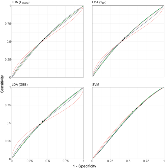
(a) Fig. S 1a

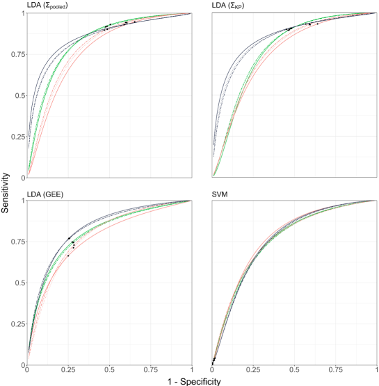
(a) Fig. S 1b

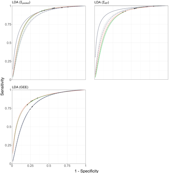
(a) Fig. S 1c

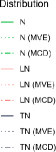
Figure S 1: Summary ROC curves showing the algorithms discriminative performance in 2000 datasets simulated from the multivariate normally ($\mathcal{N}$), lognormally ($\mathcal{LN}$) and truncated normally ($\mathcal{TN}$) distribution, respectively. The black dots and circles represent the mean and confidence region.
(a) Dataset 1: CORE-OM dataset, group variable age ($n_{0}=n_{1}=93$)
(b) Dataset 2: CORE-OM dataset, group variable hospitalisation ($n_{0}=42,n_{1}=142$)
(c) Dataset 3: CASP-19 dataset, group variable loneliness ($n_{0}=254,n_{1}=1682$)
MVE: Minimum volume ellipsoid, MCD: Minimum covariance determinant, LDA: Linear discriminant analysis, SVM: Support vector machine, $\Sigma_{pooled}$: pooled covariance matrix, $\Sigma_{KP}$: Kronecker product covariance matrix, GEE: covariance matrix of Generalized estimating equation.

(a) Fig. S 2a

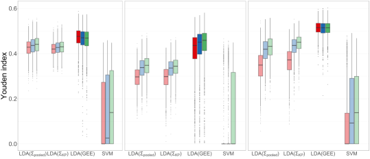
(b) Fig. S 2b

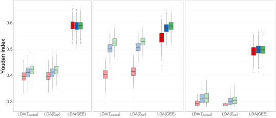
(c) Fig. S 2c

Figure S 2: Boxplots showing the distribution of Youden index estimated in the 2000 simulated datasets for the multivariate normal (left), multivariate lognormal (center) and multivariate truncated normal distribution (right). Results with the highest median value are highlighted in darker colours.
(a) Dataset 1: CORE-OM dataset, group variable age ($n_{0}=n_{1}=93$)
(b) Dataset 2: CORE-OM dataset, group variable hospitalisation ($n_{0}=42,n_{1}=142$)
(c) Dataset 3: CASP-19 dataset, group variable loneliness ($n_{0}=254,n_{1}=1682$)
MVE: Minimum volume ellipsoid, MCD: Minimum covariance determinant, LDA: Linear discriminant analysis, SVM: Support vector machine, $\Sigma_{pooled}$: pooled covariance matrix, $\Sigma_{KP}$: Kronecker product covariance matrix, GEE: covariance matrix of Generalized estimating equation.

Table S 4: Number of times the iterative algorithm for determining the optimal solution $\bm{\alpha}_{m}$ in the longitudinal SVM converged (maximum number of iterations: 100) when applied to the 2000 datasets simulated from the multivariate normally ($\mathcal{N}$), lognormally ($\mathcal{LN}$) and truncated normally ($\mathcal{TN}$) distribution based on parameter estimates obtained from Dataset 1 (CORE-OM dataset, group variable age ($n_{0}=n_{1}=93$)), Dataset 2 (CORE-OM dataset, group variable hospitalisation ($n_{0}=42,n_{1}=142$)).
MVE: Minimum volume ellipsoid, MCD: Minimum covariance determinant.

	original			MVE			MCD
	Dataset 1	Dataset 2		Dataset 1	Dataset 2		Dataset 1	Dataset 2
$\mathcal{N}$	1212	819		1191	776		1186	715
$\mathcal{LN}$	1296	1180		1235	1139		1253	1091
$\mathcal{TN}$	1244	823		1251	591		1250	520

Declarations

• Funding: No funding was received to assist with the preparation of this manuscript.

• Conflict of interest: The authors have no competing interests to declare that are relevant to the content of this article.

• Ethics approval: Not applicable.

• Availability of data and materials: Reference datasets 1 and 2 (Zeldovich, 2018) are available upon request from the corresponding author. Reference dataset 3 (Banks et al, 2021) is publicly available from the UK data service through the website https://www.elsa-project.ac.uk/accessing-elsa-data.

• Code availability: Supplementary files containing the R code used for data simulations can be found on Figshare (https://figshare.com/s/104aeb2a870a810f80bd).

References

- \bibcommenthead
- Aggarwala et al (2022) Aggarwala J, Garg R, Chatterjee S (2022) Linear Discriminant Analysis of Various Physiological and Psychological Parameters among Indian Elite Male Athletes of Different Types of Sports. Sport Mont https://doi.org/10.26773/smj.191012
- Banks et al (2021) Banks J, Batty G, Breedvelt J, et al (2021) English Longitudinal Study of Ageing: Waves 0-9, 1998-2019 [data collection]. 36th Edition. UK Data Service. SN: 5050
- Beaumont et al (2006) Beaumont J, Lix L, Yost K, et al (2006) Application of Robust Statistical Methods for Sensitivity Analysis of Health-Related Quality of Life Outcomes. Qual Life Res 15:349–56. https://doi.org/10.1007/s11136-005-2293-1
- Betz (1987) Betz NE (1987) Use of Discriminant Analysis in Counseling Psychology Research. J Couns Psychol 34:393–403. https://doi.org/10.1037/0022-0167.34.4.393
- Boedeker and Kearns (2019) Boedeker P, Kearns N (2019) Linear Discriminant Analysis for Prediction of Group Membership: A User-Friendly Primer. Adv Methods Pract Psychol Sci 2:250–263. https://doi.org/10.1177/2515245919849378
- van den Boogaart et al (2022) van den Boogaart KG, Tolosana-Delgado R, Bren M (2022) compositions: Compositional Data Analysis. CRAN. https://CRAN.R-project.org/package=compositions\bibnodot.
- Bravo et al (2021) Bravo HC, Hornik K, Theussl S (2021) Rcplex: R Interface to CPLEX. CRAN. https://CRAN.R-project.org/package=Rcplex\bibnodot.
- Brobbey (2021) Brobbey A (2021) Classification Models for Multivariate Non-normal Repeated Measures Data. [Doctoral thesis, University of Calgary] https://prism.ucalgary.ca/handle/1880/112972?show=full\bibnodot.
- Brobbey et al (2022) Brobbey A, Wiebe S, Nettel-Aguirre A, et al (2022) Repeated measures discriminant analysis using multivariate generalized estimation equations. Stat Methods Med Res 31(4):646–657. https://doi.org/10.1177/09622802211032705
- Burges (1998) Burges CJC (1998) A Tutorial on Support Vector Machines for Pattern Recognition. Data Mining and Knowledge Discovery 2:121–167. https://doi.org/10.1023/A:1009715923555
- Butler et al (1993) Butler RW, Davies PL, Jhun M (1993) Asymptotics for the Minimum Covariance Determinant Estimator. Ann Stat 21:1385 – 1400
- Castañeda Garcia and Nossek (2014) Castañeda Garcia M, Nossek J (2014) Estimation of rank deficient covariance matrices with Kronecker structure. ICASSP, IEEE International Conference on Acoustics, Speech and Signal Processing - Proceedings pp 394–398. https://doi.org/10.1109/ICASSP.2014.6853625
- Chen and Bowman (2011) Chen S, Bowman FD (2011) A novel support vector classifier for longitudinal high-dimensional data and its application to neuroimaging data. Stat Anal Data Min 4:604–611. https://doi.org/10.1002/sam.10141
- Cochrane Diagnostic Test Accuracy Working Group (2011) Cochrane Diagnostic Test Accuracy Working Group (2011) Cochrane Handbook for Systematic Reviews of Diagnostic Test Accuracy. The Cochrane Collaboration
- Cortes and Vapnik (1995) Cortes C, Vapnik VN (1995) Support-Vector Networks. Mach Learn 20:273–297. https://doi.org/10.1023/A:1022627411411
- Delacre et al (2017) Delacre M, Lakens D, Leys C (2017) Why psychologists should by default use Welch’s t-test instead of Student’s t-test. Int Rev Soc Psychol 30:92. https://doi.org/10.5334/irsp.82
- Doebler (2020) Doebler P (2020) mada: Meta-Analysis of Diagnostic Accuracy. CRAN. https://CRAN.R-project.org/package=mada\bibnodot.
- Donoho (1982) Donoho D (1982) Breakdown properties of multivariate location estimators. [unpublished PhD thesis, Department of Statistics, Harvard University, Massachusetts], https://doi.org/10.1214/aos/1176348890
- Donoho and Huber (1983) Donoho D, Huber P (1983) The notion of breakdown point. In: A Festschrift for Erich Lehmann. (edited by P. Bickel, K. Doksum, J.L. Hodges), Wadsworth, Belmont, p 157–184
- Efron and Tibshirani (1997) Efron B, Tibshirani R (1997) Improvements on Cross-Validation: The .632+ Bootstrap Method. J Am Stat Assoc 92:548–560. https://doi.org/10.2307/2965703
- Field (2017) Field A (2017) Discovering Statistics Using IBM SPSS Statistics. SAGE Publications, Thousand Oaks
- Fisher (1936) Fisher RA (1936) The use of multiple measurements in taxonomic problems. Ann Hum Genet 7:179–188
- Fletcher et al (1978) Fletcher JM, Rice WJ, Ray RM (1978) Linear Discriminant Function analysis in Neuropsychological Research: Some Uses and abuses. Cortex 14:564–577. https://doi.org/10.1016/S0010-9452(78)80031-8
- Garrett (1943) Garrett HE (1943) The discriminant function and its use in psychology. Psychometrika 8:65–79. https://doi.org/10.1007/BF02288691
- Gupta (1986) Gupta AK (1986) On a classification rule for multiple measurements. Comput Math Appl 12:301–308. https://doi.org/10.1016/0898-1221(86)90082-9
- Harbord et al (2007) Harbord R, Deeks J, Egger M, et al (2007) A unification of models for meta-analysis of diagnostic accuracy studies. Biostatistics 8:239–251. https://doi.org/10.1093/biostatistics/kxl004
- Hardin and Hilbe (2013) Hardin JW, Hilbe JM (2013) Generalized Estimating Equations. CRC Press
- Hastie et al (2004) Hastie TJ, Rosset S, Tibshirani R, et al (2004) The Entire Regularization Path for the Support Vector Machine. J Mach Learn Res 5:1391–1415
- Hawkins and McLachlan (1997) Hawkins DM, McLachlan GJ (1997) High-Breakdown Linear Discriminant Analysis. J Am Stat Assoc 92:136–143. https://doi.org/10.2307/2291457
- Huberty and Olejnik (2006) Huberty C, Olejnik S (2006) Applied MANOVA and discriminant analysis. John Wiley & Sons, Hoboken
- IBM ILOG (2021) IBM ILOG (2021) CPLEX Optimization Studio. IBM Documentation. https://www.ibm.com/docs/en/icos/20.1.0?topic=cplex\bibnodot.
- Inan (2015) Inan G (2015) JGEE: Joint Generalized Estimating Equation Solver. CRAN. https://CRAN.R-project.org/package=JGEE\bibnodot.
- Jensen et al (2021) Jensen E, Pfleger A, Lorenz L, et al (2021) A Repeated Measures Dataset on Public Responses to the COVID-19 Pandemic: Social Norms, Attitudes, Behaviors, Conspiracy Thinking, and (Mis)Information. Front Commun 6. https://doi.org/10.3389/fcomm.2021.789272
- Jiang et al (2008) Jiang B, Zhang X, Cai T (2008) Estimating the Confidence Interval for Prediction Errors of Support Vector Machine Classifiers. J Mach Learn Res 9:521–540. https://doi.org/10.5555/1390681.1390698
- Kumpulainen et al (2021) Kumpulainen P, Cardó AV, Somppi S, et al (2021) Dog activity classification with movement sensor placed on the collar. Appl Anim Behav Sci https://doi.org/10.1016/j.applanim.2021.105393
- Langlois et al (2000) Langlois F, Freeston MH, Ladouceur R (2000) Differences and similarities between obsessive intrusive thoughts and worry in a non-clinical population: study 2. Behav Res Ther 38:175–189. https://doi.org/10.1016/s0005-7967(99)00028-5
- Liang and Zeger (1986) Liang KY, Zeger SL (1986) Longitudinal data analysis using generalized linear models. Biometrika 73:13–22. https://doi.org/10.2307/2336267
- Lipsitz et al (2009) Lipsitz S, Fitzmaurice G, Ibrahim J, et al (2009) Joint generalized estimating equations for multivariate longitudinal binary outcomes with missing data: An application to AIDS data. J R Stat Soc, A: Stat Soc 172:3–20. https://doi.org/10.1111/j.1467-985X.2008.00564.x
- Lix and Sajobi (2010) Lix L, Sajobi T (2010) Discriminant Analysis for Repeated Measures Data: A Review. Front Psychol 1:146. https://doi.org/10.3389/fpsyg.2010.00146
- Lu and Zimmerman (2005) Lu N, Zimmerman D (2005) The likelihood ratio test for a separable covariance matrix. Stat Probab Lett 73:449–457. https://doi.org/10.1016/j.spl.2005.04.020
- McLanahan et al (2019) McLanahan S, Garfinkel I, Waldfogel J, et al (2019) Fragile Families and Child Wellbeing Study, Public Use, United States, 1998-2017. Inter-university Consortium for Political and Social Research [distributor]
- Morris et al (2019) Morris TP, White IR, Crowther MJ (2019) Using simulation studies to evaluate statistical methods. Stat Med 38:2074 – 2102. https://doi.org/10.1002/sim.8086
- Naik and Rao (2001) Naik DN, Rao SS (2001) Analysis of multivariate repeated measures data with a Kronecker product structured covariance matrix. J Appl Stat 28:105 – 191. https://doi.org/10.1080/02664760120011626
- Neto et al (2016) Neto E, Biessmann F, Aurlien H, et al (2016) Regularized Linear Discriminant Analysis of EEG Features in Dementia Patients. Front Aging Neurosci 8. https://doi.org/10.3389/fnagi.2016.00273
- O’Brien et al (2009) O’Brien J, Tsermentseli S, Cummins O, et al (2009) Discriminating children with autism from children with learning difficulties with an adaptation of the Short Sensory Profile. Early Child Dev Care 179:383 – 394. https://doi.org/10.1080/03004430701567926
- Rausch and Kelley (2009) Rausch J, Kelley K (2009) A comparison of linear and mixture models for discriminant analysis under nonnormality. Behav Res Methods 41:85–98. https://doi.org/10.3758/BRM.41.1.85
- Reitsma et al (2005) Reitsma J, Glas A, Rutjes A, et al (2005) Bivariate analysis of sensitivity and specificity produces informative summary measures in diagnostic reviews. J Clin Epidemiol 58:982–990. https://doi.org/10.1016/j.jclinepi.2005.02.022
- Ribeiro and Freitas (2019) Ribeiro CE, Freitas A (2019) A mini-survey of supervised machine learning approaches for coping with ageing-related longitudinal datasets
- Ripley et al (2022) Ripley B, Venables B, Bates DM, et al (2022) MASS: Support Functions and Datasets for Venables and Ripley’s MASS. CRAN. https://CRAN.R-project.org/package=MASS\bibnodot.
- Rogge and Bradbury (1999) Rogge RD, Bradbury TN (1999) Till violence does us part: the differing roles of communication and aggression in predicting adverse marital outcomes. J Consult Clin Psychol 67:340–351. https://doi.org/10.1037//0022-006x.67.3.340
- Rousseeuw (1985) Rousseeuw P (1985) Multivariate estimation with high breakdown point. Mathematical Statistics and Applications Vol B pp 283–297. https://doi.org/10.1007/978-94-009-5438-0_20
- Rousseeuw and Driessen (1999) Rousseeuw P, Driessen K (1999) A Fast Algorithm for the Minimum Covariance Determinant Estimator. Technometrics 41:212–223. https://doi.org/10.2307/1270566
- Roy and Khattree (2005a) Roy A, Khattree R (2005a) Discrimination and classification with repeated measures data under different covariance structures. Commun Stat Simul Comput 34:167–178. https://doi.org/10.1081/SAC-200047072
- Roy and Khattree (2005b) Roy A, Khattree R (2005b) On discrimination and classification with multivariate repeated measures data. J Stat Plan Inference 134:462–485. https://doi.org/10.1016/j.jspi.2004.04.012
- Rutter and Gatsonis (2001) Rutter C, Gatsonis C (2001) A hierarchical regression approach to meta-analysis of diagnostic test accuracy evaluations. Stat Med 20:2865–2884. https://doi.org/10.1002/sim.942
- Sentelle (2015) Sentelle C (2015) simplesvmpath. GitHub repository. https://github.com/csentelle/simplesvmpath.git\bibnodot.
- Sentelle et al (2016) Sentelle C, Anagnostopoulos GC, Georgiopoulos M (2016) A Simple Method for Solving the SVM Regularization Path for Semidefinite Kernels. IEEE Transactions on Neural Networks and Learning Systems 27:709–722. https://doi.org/10.1109/TNNLS.2015.2427333
- Sherry (2006) Sherry A (2006) Discriminant Analysis in Counseling Psychology Research. Couns Psychol 34:661–683. https://doi.org/10.1177/0011000006287103
- Shinba et al (2021) Shinba T, Murotsu K, Usui Y, et al (2021) Return-to-Work Screening by Linear Discriminant Analysis of Heart Rate Variability Indices in Depressed Subjects. Sensors 21. https://doi.org/10.3390/s21155177
- Stoyanov et al (2022) Stoyanov DS, Khorev VS, Paunova R, et al (2022) Resting-State Functional Connectivity Impairment in Patients with Major Depressive Episode. Int J Environ Res Public Health 19. https://doi.org/10.3390/ijerph192114045
- Talarska et al (2018) Talarska D, Tobis S, Kotkowiak M, et al (2018) Determinants of Quality of Life and the Need for Support for the Elderly with Good Physical and Mental Functioning. Med Sci Monit 24:1604–1613. https://doi.org/10.12659/MSM.907032
- Todorov (2022) Todorov V (2022) rrcov: Scalable Robust Estimators with High Breakdown Point. CRAN. https://CRAN.R-project.org/package=rrcov\bibnodot.
- Tomasko et al (2010) Tomasko L, Helms RW, Snapinn SM (2010) A discriminant analysis extension to mixed models. Stat Med 18:1249–1260. URL https://doi.org/10.1002/(SICI)1097-0258(19990530)18:10<1249::AID-SIM125>3.0.CO;2-%23
- Vapnik (1982) Vapnik V (1982) Estimation of Dependences Based on Empirical Data: Empirical Inference Science. Springer
- Vapnik (2010) Vapnik VN (2010) The nature of statistical learning theory. Springer
- Wahl et al (2016) Wahl S, Boulesteix AL, Zierer A, et al (2016) Assessment of predictive performance in incomplete data by combining internal validation and multiple imputation. BMC Med Res Methodol 16:144. https://doi.org/10.1186/s12874-016-0239-7
- Wang (2014) Wang M (2014) Generalized Estimating Equations in Longitudinal Data Analysis: A Review and Recent Developments. Advances in Statistics 2014:1–11. https://doi.org/10.1155/2014/303728
- Weber et al (2019) Weber L, Saelens W, Cannoodt R, et al (2019) Essential guidelines for computational method benchmarking. Genome Biol 20. https://doi.org/10.1186/s13059-019-1738-8
- Wilhelm and Manjunath (2022) Wilhelm S, Manjunath B (2022) tmvtnorm: Truncated Multivariate Normal and Student t Distribution. CRAN. https://CRAN.R-project.org/package=tmvtnorm\bibnodot.
- Woodruff and Rocke (1993) Woodruff DL, Rocke DM (1993) Heuristic Search Algorithms for the Minimum Volume Ellipsoid. J Comput Graph 2:69–95. https://doi.org/10.2307/1390956
- Youden (1950) Youden WJ (1950) Index for rating diagnostic tests. Cancer 3:32–35. https://doi.org/10.1002/1097-0142(1950)3:1<32::AID-CNCR2820030106>3.0.CO;2-3
- Zeldovich (2018) Zeldovich M (2018) Outcome Measurement in Russian Clinical Praxis: Clinical Outcome in Routine Evaluation – Outcome Measure (CORE-OM). [Doctoral thesis, Alpen-Adria University of Klagenfurt] https://netlibrary.aau.at/obvuklhs/content/titleinfo/5370233\bibnodot.