Decade-long timing of four GMRT discovered millisecond pulsars

.pspdf.pdfps2pdf -dEPSCrop -dNOSAFER #1

ABSTRACT

The discovery and timing follow-up of millisecond pulsars (MSPs) are necessary not just for their usefulness in Pulsar Timing Arrays (PTAs) but also for investigating their own intriguing properties. In this work, we provide the findings of the decade-long timing of the four MSPs discovered by the Giant Metre-wave Radio Telescope (GMRT), including their timing precision, model parameters, and newly detected proper motions. We compare the timing results for these MSPs before and after the GMRT upgrade in 2017, characterise the improvement in timing precision due to the bandwidth upgrade. We discuss the suitability of these four GMRT MSPs as well as the usefulness of their decade-long timing data for the PTA experiments. It may aid in the global effort to improve the signal-to-noise (S/N) of recently detected signature of gravitational waves in cross-correlation statistics of residuals of MSPs.

1 Introduction

Millisecond pulsars (MSPs) are fast rotating neutron stars that exhibit exceptional clock-like behaviour over time. Due to their rotational stability, we can probe the effects due to the interstellar medium along the line of sight as well as the effects that are intrinsic to them (e.g., Foster & Cordes (1990)). Pulsar timing (e.g., Lorimer & Kramer (2004)) is a technique that utilises the time-of-arrival (ToA) information of the pulses coming from MSPs, thus revealing precise astrometric, rotational and binary models as well as propagation effects.

The long-term timing of MSPs helps to reduce covariance between system model parameters, resulting in more precise and accurate estimation of these parameters. It can reveal higher-order effects in the system, such as the higher order derivatives of spin frequency, temporal variations in orbital motion in the case of binaries, and a change of the electron-proton plasma along the line of sight (e.g., Lorimer & Kramer (2004)). A better modelling of pulsars by taking these higher-order effects into account will result in more accurate predictions for their ToAs, making them better interstellar clocks.

Detweiler (1979) introduced the utilisation of long-term pulsar timing of MSPs to identify an isotropic stochastic gravitational wave (GW) background of cosmic origins. Its primary contributor is expected to be an ensemble of merging galaxies having supermassive black hole binaries at their centers (Burke-Spolaor et al., 2019). A pulsar timing array (PTA) is an array of well-timed MSPs with varying angular separations in the sky designed to detect the effect of nano-Hertz (nHz) GWs on the cross-correlation of timing residuals from pairs of MSPs (Hellings & Downs, 1983). The current major PTAs are the North American Nanohertz Observatory for Gravitational Waves (NANOGrav) (Jenet et al., 2009), the Parkes Pulsar Timing Array (PPTA) (Manchester, 2006), the European Pulsar Timing Array (EPTA) (Stappers et al., 2006), the Chinese Pulsar Timing Array (CPTA) (Lee, 2016), the MeerKAT Pulsar Timing Array (MPTA) (Bailes et al., 2016), and the Indian Pulsar Timing Array (InPTA) (Joshi et al., 2018).

Recently, Agazie et al. (2023) (NANOGrav), Reardon et al. (2023) (PPTA), Antoniadis et al. (2023) (EPTA $+$ InPTA), and Xu et al. (2023) (CPTA) have shown Hellings and Downs curve signatures in cross-correlation statistics of residuals for a set of MSPs. For the four PTAs, the signal-to-noise ratio (S/N) of the common correlated signal among the pairs of MSPs ranges from 3 to 5. S/N is defined here as $\rho/\sigma$ (Jenet et al., 2005). $\rho$ measures the similarity between the cross-correlation distribution of residuals (as a function of angular separation between MSPs) and the Hellings and Downs function (Hellings & Downs, 1983). $\sigma$ is the standard deviation of the cross-correlation distribution. According to Agazie et al. (2023), the next step will be to merge data sets from NANOGrav, PPTA, EPTA, and InPTA, which will consist of around 80 MSPs and a time baseline of up to 24 years. This is expected to boost the detection significance of the common correlated signal. A high S/N cross-correlation curve will clarify the source of its origin, and a larger number of pulsars may reveal anisotropy in the GW background (e.g., Hotinli et al. (2019)), polarisation structures (e.g., Sato-Polito & Kamionkowski (2022)), and so on. Along with incorporating data sets from multiple PTAs, the individual PTAs intend to improve their sensitivity to this signal by increasing the number of MSPs and the observational timing baseline.

Siemens et al. (2013) describes the equation that shows the dependency of S/N, of the cross-correlation statistics, on the number of MSPs included in the GW detection experiment, the observational cadence, the timing baseline, the timing precision achieved for individual MSPs, and the amplitude of GWs. It shows that in the intermediate signal regime (Siemens et al., 2013) the number of MSPs included in the experiment has the greatest influence on the detection significance of the common correlated GW signal, implying that identifying new MSPs which are suitable for PTAs should be of greater importance.

The Giant Meter-wave Radio telescope is an interferometer with 30 parabolic antennas and a longest baseline of 25 km. Each antenna dish has a 45 m diameter and two orthogonal polarisations (Swarup et al., 1997). The legacy GMRT system (Roy et al., 2010) is equipped with a GMRT Software Backend (GSB) with a maximum instantaneous observational bandwidth of 33 MHz within a frequency range of 120 to 1460 MHz. The upgraded GMRT (uGMRT; Reddy et al. (2017), Gupta et al. (2017)) with GMRT Wide-band Backend (GWB) became operational in 2017, which can have a maximum instantaneous observational bandwidth of 400 MHz in the same frequency range as legacy GMRT. The GMRT High Resolution Southern Sky (GHRSS) survey [Bhattacharyya et al. (2016), Bhattacharyya et al. (2019), Singh et al. (2022), Singh et al. (2023a), Sharma et al. (2023), Singh et al. (2023b)] and Fermi-directed survey [Bhattacharyya et al. (2013), Roy et al. (2015), Bhattacharyya et al. (2021), Bhattacharyya et al. (2022)] has so far discovered 12 MSPs using legacy GMRT and uGMRT systems. For the timing campaign, we have been monitoring four of these regular MSPs that are bright in the lower frequency bands of the GMRT. These four MSPs were observed using the legacy GMRT system from 2011 to 2017, and after 2017, they have been observed using the uGMRT system. Phase-coherent timing has been obtained for the GSB observations for these 4 MSPs and was reported in Bhattacharyya et al. (2019) and Bhattacharyya et al. (2022). Sharma et al. (2022) reported the phase-coherent timing with GWB observations for the same MSPs, which accounts for 2$-$4 years of observational timing baseline.

In this paper, we present the timing of GWB observations with an increased timing baseline and combine it with legacy GMRT timing data sets, resulting in around a decade-long baseline for the 4 MSPs. Section 2 and Section 3 provides the specifics of the observation and the timing technique used in this study, respectively. Section 4 reports the results from timing analysis, a comparison between GSB and GWB timing results, and a comparison of the timing residuals for the 4 GMRT MSPs with other PTAs. Section 5 summarise the findings from the decade-long timing of these 4 MSPs and the suitability of GMRT discovered MSPs and their decade long timing data sets for the PTAs.

2 Observation and data reduction

For phased array (PA) GWB observations in uGMRT band-3 (300$-$500 MHz) and band-4 (550$-$750 MHz), 70$\%$ and 80$\%$ of the array is phased, providing gains of 7 K/Jy and 8 K/Jy, respectively. An array with similar gains as GWB is phased for PA beam observations in legacy GMRT band-3 (306$-$339 MHz) and band-4 (591$-$624 MHz) (Bhattacharyya et al. (2019)). Table 1 lists the configuration for the observations in various receiver backends, dedispersion modes, frequency bands, time resolution, and antenna count. The intra-channel smearing has been corrected for coherent dedispersion mode data sets with known DM values for the observed MSPs. The residual smearing for incoherent dedispersion mode data sets is determined by 2048 (GSB) or 4096 (GWB) channels over a bandwidth of 33 and 200 MHz, respectively.

GMRT Mode Frequency Usable Time No. of Band range (MHz) bandwidth (MHz) Resolution ($\mu s$) Antennas GWB Band-3 I 300-500 135 81.92 22 GWB Band-4 I 550-750 152 81.92 25 GWB Band-3 C 300-500 135 10.24/20.48/40.96^† 22 GWB Band-4 C 550-750 152 10.24/20.48/40.96^† 25 GSB Band-3 I 306-339 30 61.44 22 GSB Band-4 I 591-624 30 61.44 25

Table 1: The table lists the details of the observational setup in different modes. C and I represent coherent and incoherent dispersion modes. In I mode, filterbank files have 2048 and 4096 channels in GSB and GWB backends, respectively.
$\dagger$ - In C mode, filterbank files have 512/1024/2048 channels in our observations. The table shows the time resolution corresponding to the filterbank with different numbers of channels.

We observed 4 GMRT-discovered MSPs, which are presented in Table 2. The table shows the mean observation time, the GMRT backend utilised, the S/N in various frequency bands, the number of epochs in various observing modes and bands, and the timing baseline for the observed MSPs. The flux density values, profiles of these MSPs at various frequencies are reported in Sharma et al. (2022). The spin period and DM are listed in the timing ephemerides table (Table 4) in Section 4.

The four MSPs were selected from the set of GMRT discovered MSPs based on the S/N ratio (provided in the same table) and the timing precision reported in Sharma et al. (2022), Bhattacharyya et al. (2022), and Bhattacharyya et al. (2019). The four MSPs are bright in GMRT band-3 and band-4, with the exception of J1120$-$3618, which has significantly lower detection significance in band-4. These MSPs have been observed roughly with a monthly cadence for the last 7.7$–$11.0 years.

	GMRT	Mean	Median S/N	No. of	Timing
MSP	Backend	Observation		Epochs	baseline
		time	Band 3   Band 4	Band 3   Band 4	(years)
		(min)		C/I          C/I
J1120$-$3618	GWB	52	64          -	19/13          -/-	4.2
	GSB			- /26          -/-	4.3
J1646$-$2142	GWB	43	70         45	26/17       13/10	4.0
	GSB			- /58        -/10	5.8
J1828$+$0625	GWB	46	35         26	19/13         4/4	3.1
	GSB			- /55         -/2	6.1
J2144$-$5237	GWB	55	48         58	27/24         4/9	5.5
	GSB			- /24          -/-	1.8

Table 2: Observational parameters of the four MSPs used in this work. The fifth column lists the number of observations collected for each MSP. It should be noted that the majority of the C and I observations indicated in the table’s fifth column were recorded simultaneously. The observation duration for MSPs with GSB and GWB backend was roughly the same.

Following the observations with the GWB, the GMRT raw PA beam data sets are converted to filterbank format, which is then incoherently dedispersed and folded with the PREPFOLD command of PRESTO (Ransom, 2011). For folding purposes, we make use of the ephimeris presented in Bhattacharyya et al. (2022), and Bhattacharyya et al. (2019). The folded data cubes (PFDs) produced by the PREPFOLD command are then converted to FITS format using the PAM command of PSRCHIVE (van Straten et al., 2012). Following the same profile bin configuration as Sharma et al. (2022), we created 128 and 64 bins for the coherent and incoherent dedispersed profile, respectively, in FITS files for all the MSPs. The FITS files are averaged to a single time integration, 64/128 bins, and 16 frequency subbands. These FITS files are then used for further timing analysis described in Section-3.

For all GSB observations, phase coherent timing has been established in Bhattacharyya et al. (2022), and Bhattacharyya et al. (2019). The GSB ToA from these works are being used directly for this study for aiding long-term timing.

3 Timing technique

This section outlines the procedure that we used to create templates for the MSPs, derive DM from each epoch observation, and produce ToAs for the timing analysis.

Procedure for creating templates: We collected all high S/N FITS files in a specified frequency band/mode for a particular MSP. We use ppalign module of “PulsePortraiture” (Pennucci (2019), Pennucci et al. (2016), and Pennucci et al. (2014)) software to create a 2-dimensional template using the FITS files. The ppalign module aligns the selected set of FITS files iteratively. This module is equipped with a robust alignment algorithm that takes into consideration not only a constant temporal phase offset between different epoch observations but also rotates each frequency subband profile of an epoch by an offset proportional to $\nu^{-2}$. Here, $\nu$ is the frequency of the corresponding frequency subband profile. This results in an aligned set of FITS files which are then averaged while keeping the frequency resolution to obtain a 2-dimensional template (function of frequency and phase bins).

For each MSP the resultant 2-dimensional template is having one time integration, 64/128 profile bins, and 16 freq-subbands. The 2-dimensional template is then frequency averaged to provide a single profile with 64/128 bins. This profile is then used as a template for the particular dedispersion mode and frequency band for that MSP. Note that we use separate templates for the two dedispersion modes and different uGMRT receiver bands for each MSP.

Deriving DM: We considered all the FITS files of a single MSP in a single band and a single dedispersion mode at a time. The template corresponding to this band, mode and MSP is used to generate freq-subband ToAs from the FITS files (having 1 time-integration, 64/128 bins, 16 frequency-subbands), resulting in 16 subband ToAs per epoch. We use the PAT command of PSRCHIVE to generate ToAs. TEMPO2 (Hobbs & Edwards, 2012) is used to fit for the DM using these subband ToAs for each epoch, keeping the other parameters fixed while fitting.

ToAs for timing: We averaged all FITS files corresponding to a specific MSP, band, and mode in frequency so that they have 1 time-integration, 64/128 bins, and 1 frequency-subband. The corresponding template for this set is used to generate a single ToA for each epoch observation. Again, we create ToAs using the PAT command of PSRCHIVE. These band-averaged ToAs are used for timing purposes.

4 Timing Results

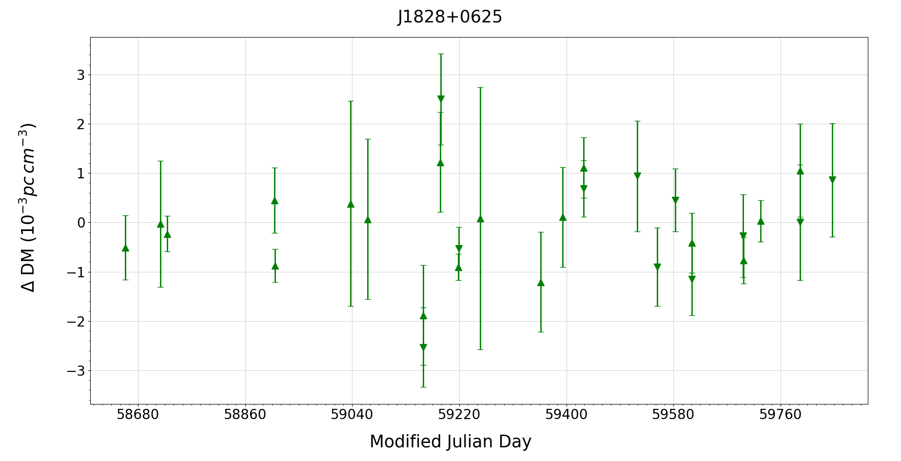
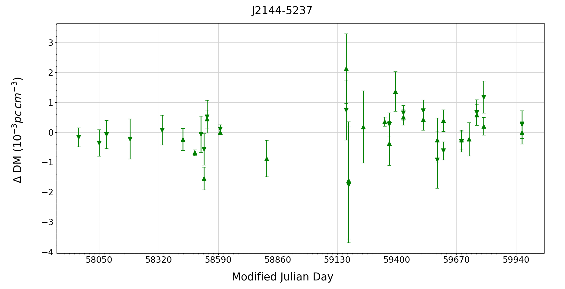
We have measured the temporal variation of DM for each of the four MSPs from the band-3 GWB data sets, and show them in each pulsar subsection below. We did not include the DM values from GWB band-4 and the GSB data sets in these plots since their error bars (GWB band-4: $\sim 5\times 10^{-3}$ pc cm^-3; GSB band-3/4: $\sim 10^{-1}$ pc cm^-3 or higher) are significantly larger than those from the GWB band-3 data sets ($\sim 5\times 10^{-4}$ pc cm^-3). Due to the very large DM error bars in the GSB data sets, we did not consider the DM variations with time for any of the MSPs to treat GSB and GWB data sets equally when doing timing. Instead, we used a global DM for the combined timing of band-3 + band-4 and GSB+GWB data sets (named GSB+GWB from now on) of each MSP.

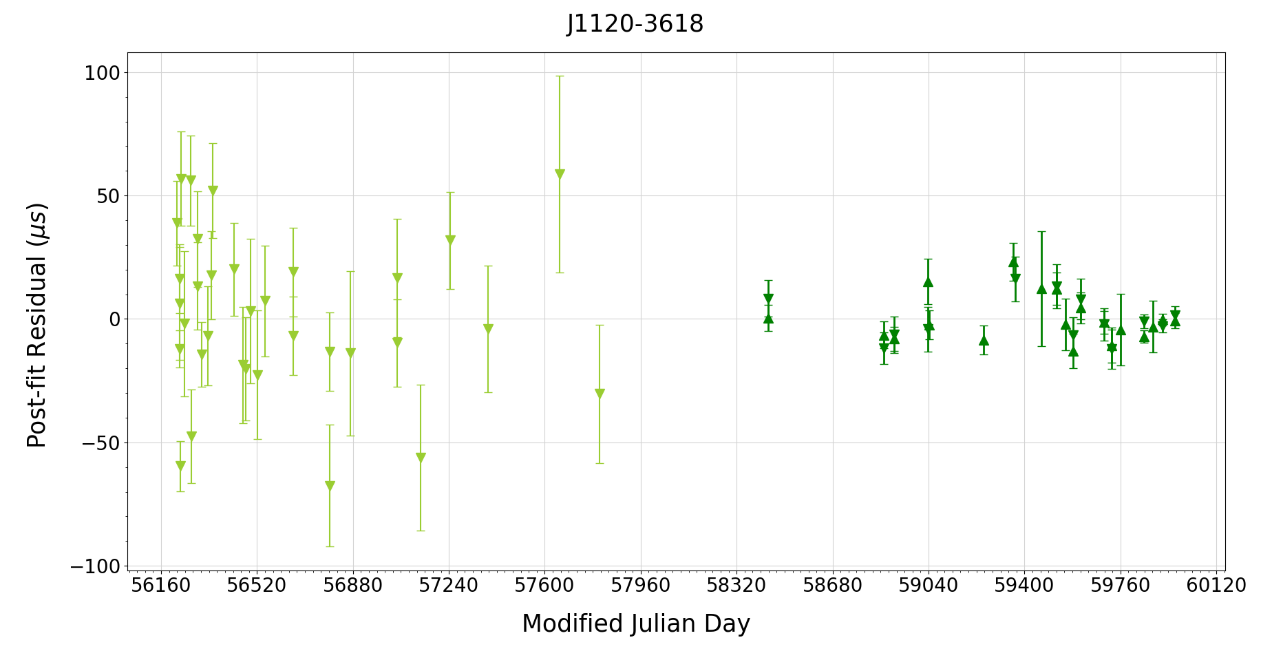
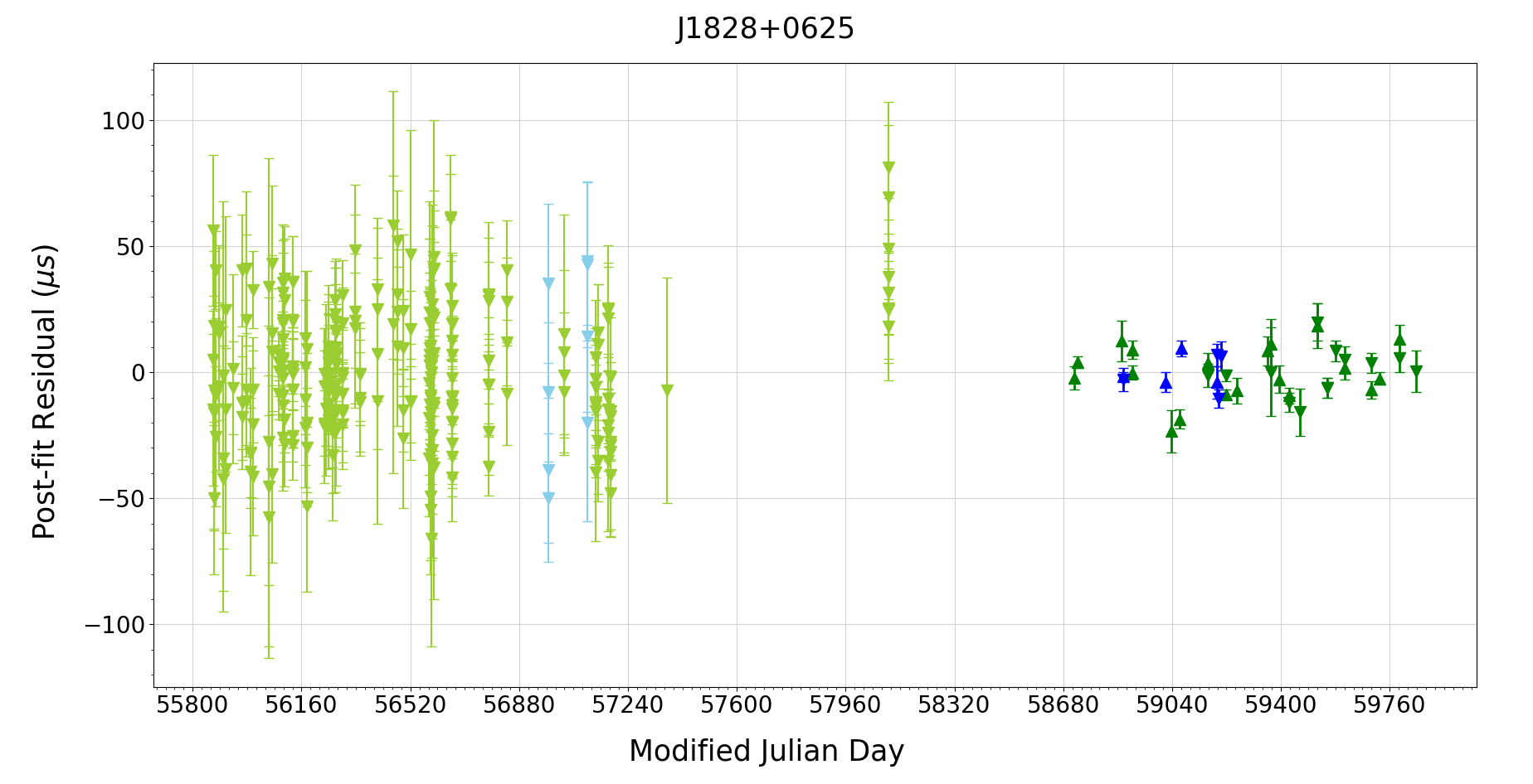
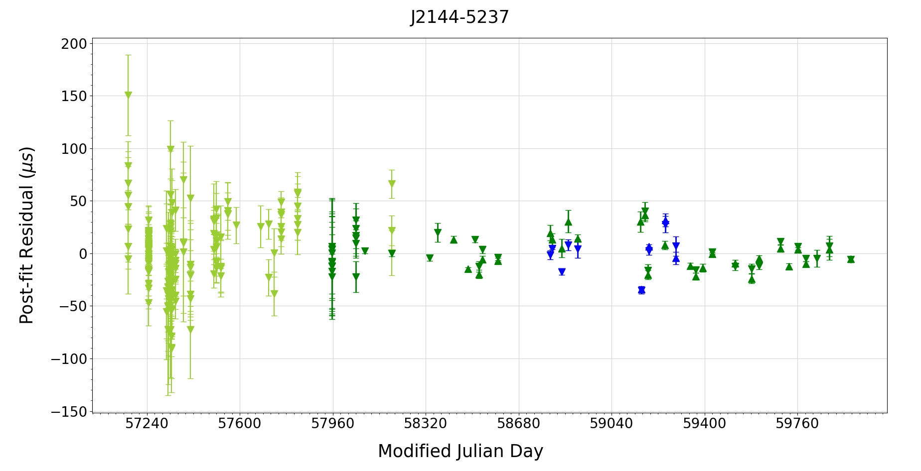
Table 3 shows the number of ToAs corresponding to individual frequency bands and receiver backends for each MSP, as well as the median ToA uncertainty and the root-mean-square (RMS) of post-fit timing residuals obtained from the individual GSB, GWB, and GSB+GWB timing for these MSPs. We show the post-fit residuals for each MSPs, corresponding to GSB+GWB timing, in each pulsar subsection below. Table 4 shows the timing ephimerides and derived parameters obtained from phase-coherent timing of GSB+GWB.

4.1 J1120$-$3618

J1120$-$3618 is a binary MSP with a spin-period of $\sim$5.56 ms, an orbital period of $\sim$5.66 days, and a DM of $\sim$45.12 $pc\,cm^{-3}$. The timing precision obtained in individual GWB and GSB timing is 6.1 and 27.0 $\mu s$ respectively, each spanning more than 4 years of baseline. We achieved an overall timing precision of 10.5 $\mu s$ after combining the GSB and GWB timing data sets (spanning 10.3 years), which is clearly limited by the larger error bars of ToAs in GSB timing data.

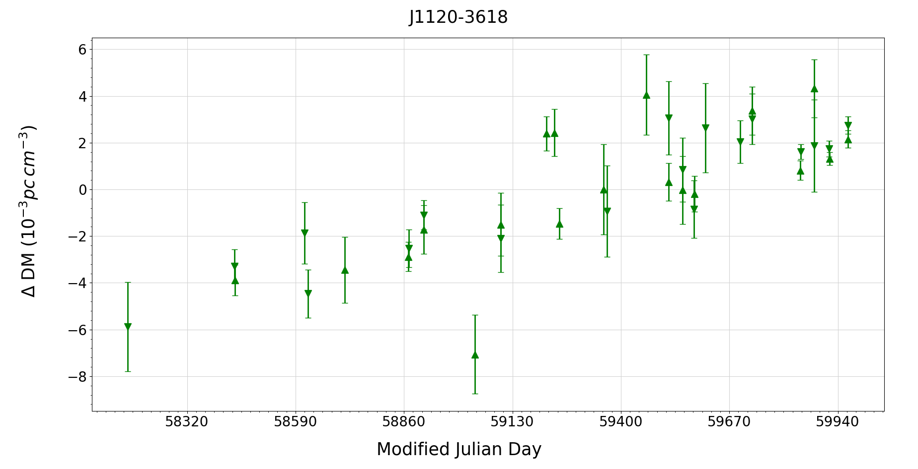
This MSP’s line of sight is crossing an electron-rich medium for the last 4–5 years, as indicated by its DM trend seen in GWB band-3. Its DM value has increased by 8.6$\times$10^-3 $pc\,cm^{-3}$ from February 2018 to January 2023 while the median DM error bar for this MSP in GWB band-3 is 1.0$\times$10^-3 $pc\,cm^{-3}$.

Figure 1: Figure showing DM variation with time for the MSP J1120$-$3618 in GWB band-3 of the uGMRT. Up and down triangles represent coherently and incoherently dedispersed data, respectively.

Figure 2: Post-fit timing residuals vs MJD for MSP J1120$-$3618. Yellow green and green colors are used for GSB band-3 and GWB band-3, respectively. Up and down triangles represent coherently and incoherently de-dedispersed data sets, respectively.

We measure a total proper motion for this MSP, for the first time, of 6.0(6) $mas/yr$ from GSB+GWB timing, and individually 5.2(6) $mas/yr$ in right ascension (RA) and 2.8(7) $mas/yr$ in declination (DEC). The proper motion for J1120$-$3618 falls within the typical proper motion range for known MSPs [few tens of $mas/yr$; ATNF pulsar catalogue (Manchester et al., 2005)].

We estimate the distance to this MSP using its DM, position, and the galactic electron density models NE2001 (Cordes & Lazio, 2002) and YMW16 (Yao et al., 2017), which result in a distance of 1.75 and 0.95 $kpc$, respectively. Using these estimates and the proper motion value for this MSP, we calculate transverse velocities of 49 $km/s$ (for 1.74 $kpc$; NE2001) and 27 $km/s$ (for 0.95 $kpc$; YMW16). These transverse velocity values are significantly lower than the maximum expected space velocity of the MSPs ($\sim$270 $km/s$) in the scenario of spherically symmetric supernova explosions, suggesting that this MSP did not experience an asymmetric kick during its recoiling phase (Tauris & Bailes, 1996).

The timing-fit for J1120$-$3618 yields a spin-period derivative (P1) of 9.4(3) $\times$ 10^-22 s/s, an order of magnitude less than the other three MSPs in this work. It has an intrinsic spin-period derivative (Toscano et al., 1999) of $\sim$5.5 $\times$ 10^-22 s/s ($\sim$0.6 P1) [determined using Equation 2 of Toscano et al. (1999), proper motion, and the distance measurements from the YMW16 model]. The P1-value of J1120$-$3618 is the fifth smallest of all MSPs currently known.

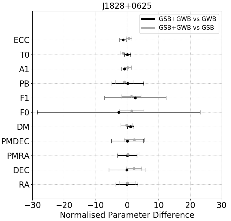
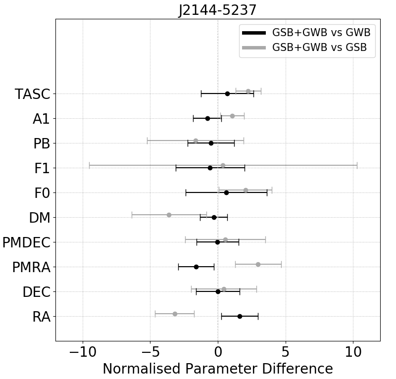
Figure 3 shows a comparison of fitted model parameters from GWB, GSB, and GSB+GWB timing for this MSP. Commonly fitted model parameters (listed in Figure 3) obtained from GSB+GWB timing are on average 1.1 and 3.6 times more precise than individual GWB and GSB timing, respectively. The model parameters from GSB+GWB timing are consistent with individual GWB or GSB timing within $\pm 1\sigma$, where $\sigma$ is the error bar of the fitted model parameter from either GWB or GSB.

Figure 3: Figures showing a comparison of our fitted timing models for J1120$-$3618. The y-axis shows the name of the fitted parameter.
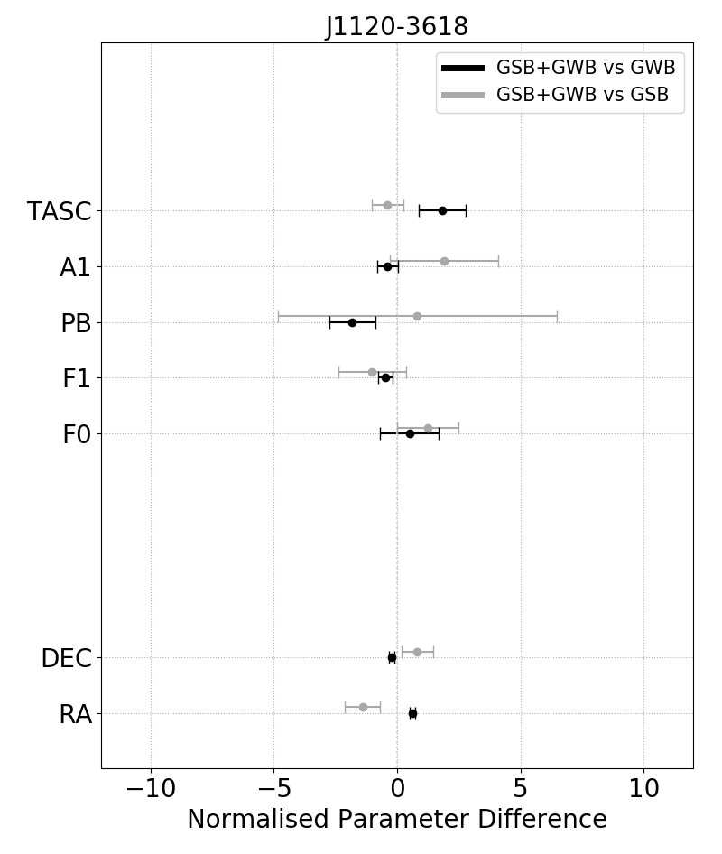
Black color points/error-bars: The x-axis shows the differences of the fitted parameter (astrometric, spin, and binary) values between GSB+GWB timing and only GWB timing normalized by the uncertainties of GWB, i.e., $(X_{GSB+GWB}-X_{GWB})/\sigma_{X}^{GWB}$ where X is the MSP’s model parameter. The error bars have a length equal to the ratio of parameter uncertainties from GWB and GSB+GWB models, i.e., $\sigma_{X}^{GWB}/\sigma_{X}^{GSB+GWB}$.
Dark gray color points/error-bars: The x-axis shows the difference of parameter values between GSB+GWB timing and only GSB timing normalized by the uncertainties of GSB, i.e., $(X_{GSB+GWB}-X_{GSB})/\sigma_{X}^{GSB}$. The error bar length in this case is $\sigma_{X}^{GSB}/\sigma_{X}^{GSB+GWB}$.

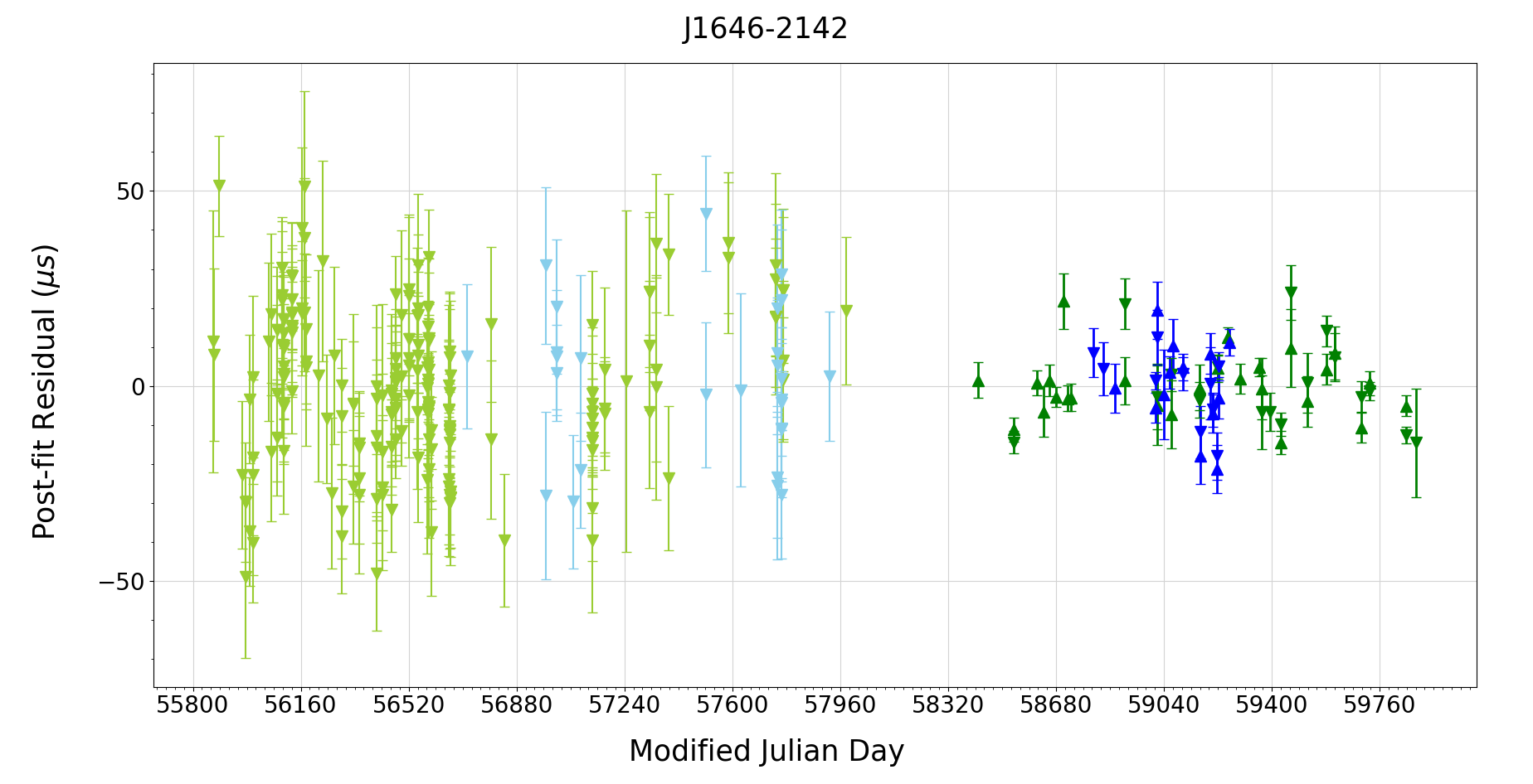
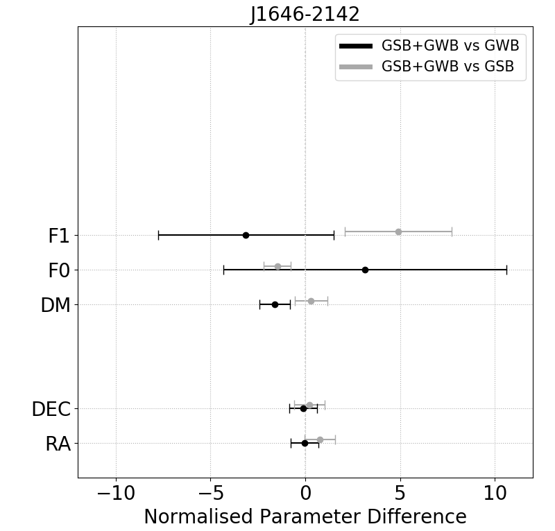
4.2 J1646$-$2142

J1646$-$2142 is an isolated MSP with a spin-period of $\sim$5.85 ms and a DM of $\sim$29.74 $pc\,cm^{-3}$. Timing precision in GWB and GSB timing are 7.3 and 15.7 $\mu s$, respectively. With combined GSB and GWB timing data, we achieved a timing precision of 11.1 $\mu s$ for a span of 11.0 years.

The median DM uncertainty for this MSP in GWB band-3 and band-4 is 6.5$\times$10^-4 and 5.1 $\times$10^-3 $\,pc\,cm^{-3}$, respectively. We see an overall DM change of less than $\pm$3 $\sigma_{DM}$ from July 2017 to October 2022, where $\sigma_{DM}$ is the median DM uncertainty in GWB band-3.

Figure 4: Figure showing DM variation with time for the MSP J1646$-$2142 in GWB band-3 of the uGMRT. The rest of the plotting approach is the same as in Figure 1.

Figure 5: Post-fit timing residuals vs MJD for MSP J1646$-$2142. Yellow green, green, sky blue, and blue colors are used for GSB band-3, GWB band-3, GSB band-4, and GWB band-4, respectively. Up and down triangles represent coherently and incoherently de-dedispersed data sets, respectively.

The GSB+GWB timing fit resulted in insignificant detection of proper motion; therefore, we excluded its fitting in timing. Figure 6 shows differences in model parameters and their precision in GSB+GWB timing against individual GWB and GSB timing. We see an average improvement in model parameter precision of 5.7 and 2.4 times in GSB+GWB timing when compared individually to GWB and GSB timing, respectively. The model parameters from GSB+GWB timing are consistent with individual GSB or GWB timing within $\pm 1\sigma$, where $\sigma$ is the error bar of the fitted model parameter from either GSB or GWB.

Figure 6: Figure showing a comparison of the fitted timing models for J1646$-$2142 in GSB+GWB timing to individual GWB and GSB timing. The plotting style is the same to Figure 3.

4.3 J1828$+$0625

J1828$+$0625 is a binary MSP with a spin-period of $\sim$3.63 ms, an orbital period of $\sim$77.92 days, and a DM of $\sim$22.42 $pc\,cm^{-3}$. We achieved timing precision of 6.2 and 20.9 $\mu s$ in individual timing of the GWB and GSB data sets, respectively. The combined GSB+GWB timing resulted in a timing precision of around 11.8 $\mu s$ for a span of 10.9 years.

The median DM uncertainty of this MSP in GWB band-3 and band-4 is 8.1$\times$10^-4 and 5.2$\times$10^-3 $pc\,cm^{-3}$, respectively. We find that the DM variation for this MSP is confined within $\pm$3 $\sigma_{DM}$ from June 2019 to September 2022, where $\sigma_{DM}$ is the median DM uncertainty in GWB band-3.

Figure 7: Figure showing DM variation with time for the MSP J1828$+$0625 in GWB band-3 of the uGMRT. The rest of the plotting approach is the same as in Figure 1.

Figure 8: Post-fit timing residuals vs MJD for MSP J1828$+$0625. The rest of the plotting approach is the same as in Figure 5.

For this MSP, we estimated a total proper motion of 14.4(2) $mas/yr$, which is well within $\pm$2$\sigma$ of the values reported in Bhattacharyya et al. (2022). The increased timing span with precise GWB ToAs allows to derive the proper motion with at least 5 times higher precision than the values reported in Bhattacharyya et al. (2022) using only GSB data.

The distance estimates for this MSP using the NE2001 and YMW16 models are 1.12 and 1.00 $kpc$, respectively. Proper motion and these distances give a transverse velocity of 77 km/s (for 1.12 $kpc$; NE2001) and 68 km/s (for 1.00 $kpc$; YMW16) for this MSP, which is comparable to the transverse velocities of J1120$–$3618 and suggests the absence of an asymmetric kick during recoiling. The timing fit for this MSP resulted in a precise P1 value of 4.6882(9) $\times$ 10^-21 s/s. Using its transverse velocity and distance (for YMW16), the intrinsic spin period derivative is estimated to be $\sim$2.7 $\times$ 10^-21 s/s ($\sim$0.6 P1).

Figure 9 compares model parameters obtained from GSB+GWB timing to individual GSB or GWB timing. The model parameters obtained from GSB+GWB timing are on average 10.5 times more precise than individual GWB timing while being 4.5 times more precise than individual GSB timing. The model parameters resulting from GSB+GWB timing are in agreement with the parameters obtained from individual GWB or GSB timing within $\pm$1 $\sigma$, where $\sigma$ is the error in model parameter obtained from individual timing of GWB or GSB data sets.

Figure 9: Figure showing a comparison of the fitted timing models for J1828$+$0625 in GSB+GWB timing to individual GWB and GSB timing. The plotting style is the same to Figure 3.

4.4 J2144$-$5237

J2144$-$5237 is a binary MSP with a spin-period of $\sim$5.04 ms, an orbital period of $\sim$10.58 days, and a DM of $\sim$19.55 $pc\,cm^{-3}$. The timing precision achieved in individual timing of GWB and GSB data is 9.0 and 17.1 $\mu s$, respectively, whereas combined GSB+GWB timing resulted in a timing precision of 10.6 $\mu s$ over a 7.7-year span.

The median DM uncertainty for this MSP in GWB band-3 and band-4 is 4.3$\times$10^-4 and 5.8$\times$10^-3 $pc\,cm^{-3}$, respectively. We see small variations in DM from July 2017 to January 2023, which are contained within $\pm$3 $\sigma_{DM}$, where $\sigma_{DM}$ is the DM uncertainty in GWB band-3.

Figure 10: Figure showing DM variation with time for the MSP J2144$-$5237 in GWB band-3 of the uGMRT. The rest of the plotting approach is the same as in Figure 1.

Figure 11: Post-fit timing residuals vs MJD for MSP J2144$-$5237. The rest of the plotting approach is the same as in Figure 5. However, this MSP did not have GSB band-4 data available.

Individual GSB and GWB timing resulted in unreliable proper motion values with large error bars. We find proper motion for this MSP (9.8(5) $mas/yr$) for the first time using combined GSB+GWB timing.

The NE2001 and YMW16 models (together with DM and position) gave distance estimates of 0.80 and 1.66 $kpc$ for this MSP, respectively. The resulting transverse velocities are 37 $km/s$ (for 0.80 $kpc$, NE2001) and 77 $km/s$ (for 1.66 $kpc$, YMW16), respectively. These numbers are comparable to the transverse velocities of MSPs J1120$–$3618 and J1828$–$0625, and suggest a symmetric supernova explosion for this MSP as well. The timing fit for this MSP resulted in a P1 value of 9.055(3) $\times$ 10^-21 s/s, from which the intrinsic spin period derivative is calculated to be $\sim$5.9 $\times$ 10^-21 s/s ($\sim$0.6 P1).

Figure 12 compares the model parameters obtained from GSB+GWB timing with those obtained from individual GWB and GSB timing. The model parameters obtained from GSB+GWB timing are on average 3.4 and 5.7 times more precise than parameters in individual GWB and GSB timing, respectively. Also, the model parameter values obtained from GSB+GWB timing are within $\pm$1 $\sigma$ of the model parameters obtained from individual GWB and GSB timing, where $\sigma$ is the error in model parameter obtained from individual timing of GWB or GSB data sets.

Figure 12: Figure showing a comparison of the fitted timing models for J2144$-$5237 in GSB+GWB timing to individual GWB and GSB timing. The plotting style is the same to Figure 3.

Parameter Backend Band J1120$-$3618 J1646$-$2142 J1828$+$0625 J2144$-$5237 GWB B3 33 43 32 51 $N_{ToA}$ B4 - 23 8 13 GSB B3 32 192 273 185 B4 - 27 8 - Median GWB B3 6.74 4.09 4.51 3.28 $\sigma_{ToA}$ B4 - 5.97 4.18 4.32 ($\mu$s) GSB B3 19.52 16.56 22.19 20.55 B4 - 17.14 30.60 - Post-fit GWB B3+B4^† 6.1 7.3 6.2 9.0 timing res- GSB 27.0 15.7 20.9 17.1 iduals ($\mu$s) GSB+GWB 10.5 11.1 11.8 10.6

Table 3: The table lists the number of ToAs, median ToA uncertainties, and post-fit timing residuals for each MSP in both frequency bands and for both (and combination of) receiver backend data sets. B3 and B4 represent band-3 and band-4, respectively. The $\dagger$ on B4 in the third and last column and row is to indicate “whenever available”.

Fitted parameters J1120$-$3618 J1646$-$2142 J1828$+$0625 J2144$-$5237 RA (hh:mm:ss.s) 11:20:23.3553(4) 16:46:18.6341(3) 18:28:28.95501(5) 21:44:35.6453(7) PMRA (mas/yr) 5.2(6) -14.0(2) 5.4(3) DEC (dd:mm:ss.s) -36:19:40.477(7) -21:42:02.51(3) +06:25:09.793(1) -52:37:07.41(1) PMDEC (mas/yr) 2.8(7) -3.0(2) -8.2(5) F0 (s^-1) 179.95266943563(6) 170.849405719173(5) 275.667196397883(4) 198.35548314683(2) F1 (s^-2) -3.03(9)e-17 -2.4248(3)e-16 -3.5627(7)e-16 -3.563(1)e-16 F2 (s^-3) 3.0(5)e-26 DM (pc cm^-3) 45.128(3) 29.74000(9) 22.4165(1) 19.5500(2) BINARY ELL1 ISOLATED DD ELL1 PB (days) 5.659945229(3) 77.92496858(2) 10.580318287(5) A1 (lt-s) 4.304023(3) 34.888407(1) 6.361098(2) T0 (MJD) 57546.579(8) TASC (MJD) 56225.015639(2) 57497.7855778(7) OM (degrees) 230.35(3) ECC 9.795(8)e-05 START-FINISH (MJD) 56220-59965 55869-59881 55869-59848 57168-59966 Reference MJD 57805 57924 58103 58539 NTOA 65 285 321 249 Number of Fit Parameters 11 6 13 11 Post-fit timing residuals ($\mu$s) 10.462 11.095 11.814 10.550 Units TCB TDB TDB TDB EPHEM DE200 DE200 DE405 DE200 TIMEEPH IF99 FB90 FB90 FB90 Derived Parameters P0 (ms) 5.557016759664(2) 5.8531078629779(2) 3.62756255755819(5) 5.0414537785161(4) Transverse velocity (km/s) [YMW16] 27 68 77 Measured P1 (s/s) 9.4(3)e-22 8.307(1)e-21 4.6882(9)e-21 9.055(3)e-21 Intrinsic P1 (s/s) [YMW16] 5.5e-22 2.7e-21 5.9e-21 Surface Magnetic field (10⁸ Gauss) 0.730 2.231 1.320 2.162 Median Companion Mass ($M_{\odot}$) 0.2161 0.3180 0.2099 Spin-down Luminosity (10³³ erg s^-1) 0.2157 1.6364 3.8793 2.7914 Total time span (years) 10.253 10.987 10.894 7.662

Table 4: The table lists the parameters that have been fitted or derived for a specific MSP along with the units of measurement (if applicable). The parameters and their uncertainty (if applicable) values are derived from band-3+band-4 (whenever available) and GSB+GWB timing fit. The parameter definitions are the same as in Table 2 and 3 of the tempo2 manual, which is available at https://www.jb.man.ac.uk/~pulsar/Resources/tempo2_manual.pdf.

4.5 Comparison with MSPs currently included in PTAs

The International pulsar timing array (IPTA; Verbiest et al. (2016), Perera et al. (2019)) combines timing data from three major PTAs: NANOGrav, PPTA, and EPTA, with the goal of improving timing precision for individual MSPs. IPTA second data release Perera et al. (2019) reported timing analyses of 65 MSPs, providing the model parameters and timing residuals obtained for each MSP. In Figure 13, we plotted the RMS of timing residuals obtained for the 65 IPTA MSPs and 4 GMRT MSPs in GSB+GWB timing.

Figure 13: Top panel: Figure showing the timing precision of 65 IPTA MSPs and four GMRT discovered MSPs. Here, we’ve used the timing precision for the IPTA MSPs (green color) listed in appendix A of Perera et al. (2019). For the GMRT discovered MSPs, we plotted the timing precision (magenta color) obtained from GSB+GWB timing given in Table 3 of this work. On the x-axis, MSPs are sorted in decreasing order of timing precision. Bottom panel: Timing precision of 14 PTA MSPs monitored by InPTA (using uGMRT) and four GMRT discovered MSPs. Here, we’ve used the timing precision for the InPTA MSPs (black color) listed in Figure 5 of Tarafdar et al. (2022). For the GMRT discovered MSPs, we plotted the timing precision (dark-gray color) obtained from only GWB timing given in Table 3 of this work. Again, MSPs are sorted in decreasing order of timing precision on the x-axis.

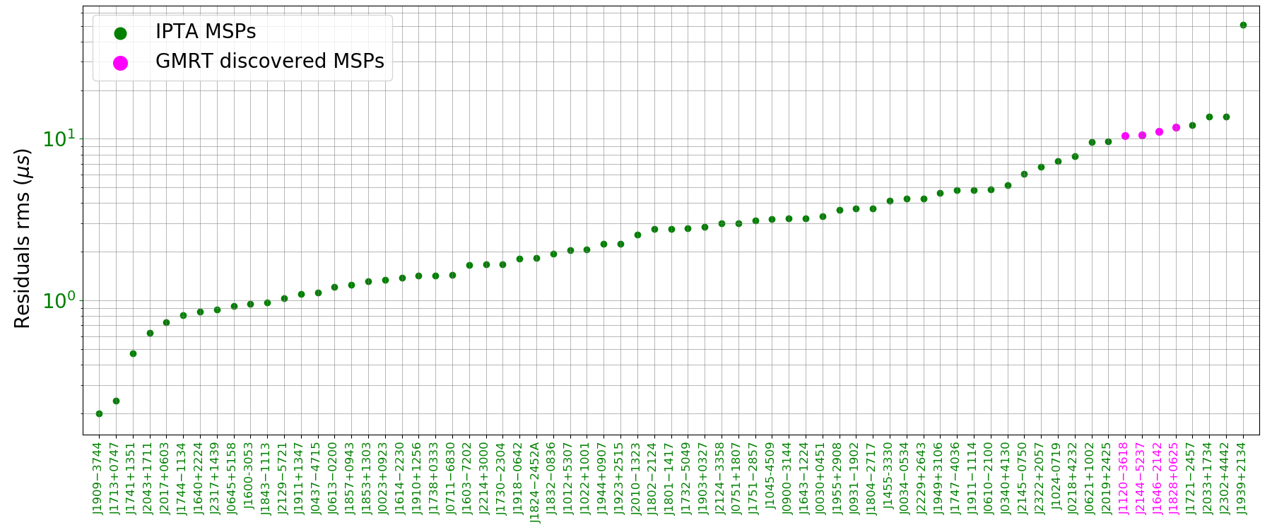
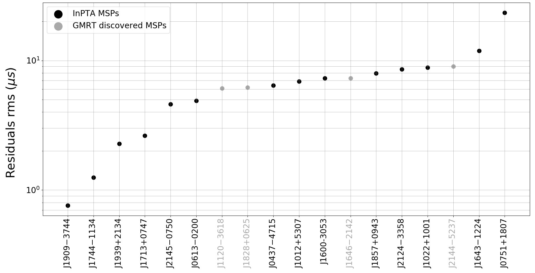
The 4 GMRT discovered MSPs fall inside timing precision range for the IPTA MSPs. We note that the RMS timing residuals obtained from individual GWB timing are (on average) 1.5 times less than the RMS timing residuals obtained from GSB+GWB timing. Therefore, considering solely the GWB timing precision makes them even more promising candidates for PTA experiments. Moreover, Tarafdar et al. (2022)(InPTA) reported the RMS timing residual of 14 well-timed PTA MSPs (observed with uGMRT) from GWB timing observations for a span of $\sim$ four years. The timing precision for these bright PTA MSPs at the uGMRT ranges between 0.76$-$23.4 $\mu$s (Figure 13; bottom panel). This clearly illustrates that the timing precision of the four GMRT-discovered MSPs (based on GWB observations) is well within the range of PTA MSPs over a similarly sized timing span.

5 Summary

In this work, we compared the timing results of the 4 GMRT-discovered MSPs for GWB (spanning 3.1$–$5.5 years), GSB (spanning 1.8$–$6.1 years), and GSB+GWB (covering 7.7$–$11.0 years) combined observations. The RMS of timing residuals obtained from GSB+GWB timing is on average $\sim$1.6 times higher than individual GWB timing but $\sim$1.8 times (on average) lower than the residual’s RMS obtained from GSB timing. The fitted model parameters in GSB+GWB timing are on average 5 and 4 times more precise than those in individual GWB and GSB timing, respectively. Model parameters from GSB+GWB timing are consistent with individual GWB and GSB timing within $\pm 1$$\sigma$, where $\sigma$ is the error in model parameter obtained from individual timing of GWB or GSB observations.

We presented DM variations for the 4 MSPs derived from GWB observations. We find that the line of sight for J1120$-$3618 crosses an electron-rich medium. We see an $\sim$9$\,\sigma_{DM}$ increase in the DM value for this MSP during the GWB observations period of 4.2 years, where $\sigma_{DM}$ is the median DM uncertainty. For the remaining three MSPs, the change in DM values is contained within $\pm 3$ $\sigma_{DM}$.

We detected proper motion for the first time for J1120$-$3618 (6.0(6) $mas/yr$) and J2144$-$5237 (9.8(5) $mas/yr$). For J1828$-$0625, we detect a proper motion of 14.4(2) $mas/yr$, which is at least five times more precise than that reported in Bhattacharyya et al. (2022). The transverse velocity for the three MSPs, calculated from these proper motion values and the distance estimates derived from NE2001 and YMW16, falls within the range expected for the MSPs (e.g., Hobbs et al. (2005)).

Finally, we compared the timing precision achieved for the four GMRT MSPs to that of 65 IPTA MSPs reported in the second IPTA data release (Perera et al., 2019) and with 14 MSPs reported in first data release of InPTA (Tarafdar et al., 2022). The GMRT MSPs fall within the timing precision range of the IPTA MSPs and InPTA observed MSPs, making them potential candidates for PTA experiments. The decade-long timing data for the four GMRT MSPs utilised in this study may be useful in the ongoing global effort to aid to the detection significance of the common correlated signal recently detected by multiple PTAs.

6 Acknowledgments

We gratefully acknowledge the Department of Atomic Energy, Government of India, for its assistance under project no. 12-R$\&$D-TFR-5.02-0700. The GMRT is run by the National Centre for Radio Astrophysics - Tata Institute of Fundamental Research.

References

- Agazie et al. (2023) Agazie, G., Anumarlapudi, A., Archibald, A. M., et al. 2023, ApJ, 951, L8. doi:10.3847/2041-8213/acdac6
- Alam et al. (2021) Alam, M. F., Arzoumanian, Z., Baker, P. T., et al. 2021, ApJS, 252, 5. doi:10.3847/1538-4365/abc6a1
- Antoniadis et al. (2023) Antoniadis, J., Babak, S., Bak Nielsen, A.-S., et al. 2023, arXiv:2306.16224. doi:10.48550/arXiv.2306.16224
- Bailes et al. (2021) Bailes, M., Berger, B. K., Brady, P. R., et al. 2021, Nature Reviews Physics, 3, 344. doi:10.1038/s42254-021-00303-8
- Bailes et al. (2016) Bailes, M., Barr, E., Bhat, N. D. R., et al. 2016, MeerKAT Science: On the Pathway to the SKA, 11. doi:10.22323/1.277.0011
- Bhattacharyya et al. (2013) Bhattacharyya, B., Roy, J., Ray, P. S., et al. 2013, ApJ, 773, L12. doi:10.1088/2041-8205/773/1/L12
- Bhattacharyya et al. (2016) Bhattacharyya, B., Cooper, S., Malenta, M., et al. 2016, ApJ, 817, 130. doi:10.3847/0004-637X/817/2/130
- Bhattacharyya et al. (2019) Bhattacharyya, B., Roy, J., Stappers, B. W., et al. 2019, ApJ, 881, 59. doi:10.3847/1538-4357/ab2bf3
- Bhattacharyya et al. (2021) Bhattacharyya, B., Roy, J., Johnson, T. J., et al. 2021, ApJ, 910, 160. doi:10.3847/1538-4357/abe4d5
- Bhattacharyya et al. (2022) Bhattacharyya, B., Roy, J., Freire, P. C. C., et al. 2022, ApJ, 933, 159. doi:10.3847/1538-4357/ac74b6
- Burke-Spolaor et al. (2019) Burke-Spolaor, S., Taylor, S. R., Charisi, M., et al. 2019, aapr, 27, 5. doi:10.1007/s00159-019-0115-7
- Cordes & Lazio (2002) Cordes, J. M. & Lazio, T. J. W. 2002, astro-ph/0207156. doi:10.48550/arXiv.astro-ph/0207156
- Cordes et al. (2006) Cordes, J. M., Freire, P. C. C., Lorimer, D. R., et al. 2006, ApJ, 637, 446. doi:10.1086/498335
- Detweiler (1979) Detweiler, S. 1979, apj, 234, 1100. doi:10.1086/157593
- Foster & Cordes (1990) Foster, R. S. & Cordes, J. M. 1990, ApJ, 364, 123. doi:10.1086/169393
- Gupta et al. (2017) Gupta, Y., Ajithkumar, B., Kale, H. S., et al. 2017, Current Science, 113, 707. doi:10.18520/cs/v113/i04/707-714
- Hellings & Downs (1983) Hellings, R. W. & Downs, G. S. 1983, apjl, 265, L39. doi:10.1086/183954
- Hobbs et al. (2005) Hobbs, G., Lorimer, D. R., Lyne, A. G., et al. 2005, MNRAS, 360, 974. doi:10.1111/j.1365-2966.2005.09087.x
- Hobbs & Edwards (2012) Hobbs, G. & Edwards, R. 2012, Astrophysics Source Code Library. ascl:1210.015
- Hotinli et al. (2019) Hotinli, S. C., Kamionkowski, M., & Jaffe, A. H. 2019, The Open Journal of Astrophysics, 2, 8. doi:10.21105/astro.1904.05348
- Joshi et al. (2018) Joshi, B. C., Arumugasamy, P., Bagchi, M., et al. 2018, Journal of Astrophysics and Astronomy, 39, 51. doi:10.1007/s12036-018-9549-y
- Jenet et al. (2005) Jenet, F. A., Hobbs, G. B., Lee, K. J., et al. 2005, ApJ, 625, L123. doi:10.1086/431220
- Jenet et al. (2009) Jenet, F., Finn, L. S., Lazio, J., et al. 2009, arXiv:0909.1058
- Keith et al. (2010) Keith, M. J., Jameson, A., van Straten, W., et al. 2010, MNRAS, 409, 619. doi:10.1111/j.1365-2966.2010.17325.x
- Lee (2016) Lee, K. J. 2016, Frontiers in Radio Astronomy and FAST Early Sciences Symposium 2015, 502, 19
- Liu et al. (2014) Liu, K., Desvignes, G., Cognard, I., et al. 2014, MNRAS, 443, 3752. doi:10.1093/mnras/stu1420
- Lorimer & Kramer (2004) Lorimer, D. R. & Kramer, M. 2004, Handbook of pulsar astronomy, by D.R. Lorimer and M. Kramer. Cambridge observing handbooks for research astronomers, Vol. 4. Cambridge, UK: Cambridge University Press, 2004
- Manchester et al. (2005) Manchester, R. N., Hobbs, G. B., Teoh, A., et al. 2005, AJ, 129, 1993. doi:10.1086/428488
- Manchester (2006) Manchester, R. N. 2006, Chinese Journal of Astronomy and Astrophysics Supplement, 6, 139
- McMullin et al. (2007) McMullin, J. P., Waters, B., Schiebel, D., et al. 2007, Astronomical Data Analysis Software and Systems XVI, 376, 127 (uGMRT)
- Mohan & Rafferty (2015) Mohan, N. & Rafferty, D. 2015, Astrophysics Source Code Library. ascl:1502.007
- Pennucci (2019) Pennucci, T. T. 2019, ApJ, 871, 34. doi:10.3847/1538-4357/aaf6ef
- Pennucci et al. (2016) Pennucci, T. T., Demorest, P. B., & Ransom, S. M. 2016, Astrophysics Source Code Library. ascl:1606.013
- Pennucci et al. (2014) Pennucci, T. T., Demorest, P. B., & Ransom, S. M. 2014, ApJ, 790, 93. doi:10.1088/0004-637X/790/2/93
- Perera et al. (2019) Perera, B. B. P., DeCesar, M. E., Demorest, P. B., et al. 2019, MNRAS, 490, 4666. doi:10.1093/mnras/stz2857
- Prasad & Chengalur (2012) Prasad, J. & Chengalur, J. 2012, Experimental Astronomy, 33, 157. doi:10.1007/s10686-011-9279-5
- Ransom (2011) Ransom, S. 2011, Astrophysics Source Code Library. ascl:1107.017
- Reardon et al. (2023) Reardon, D. J., Zic, A., Shannon, R. M., et al. 2023, ApJ, 951, L6. doi:10.3847/2041-8213/acdd02
- Reddy et al. (2017) Reddy, S. H., Kudale, S., Gokhale, U., et al. 2017, Journal of Astronomical Instrumentation, 6, 1641011-336. doi:10.1142/S2251171716410117
- Roy et al. (2010) Roy, J., Gupta, Y., Pen, U.-L., et al. 2010, Experimental Astronomy, 28, 25. doi:10.1007/s10686-010-9187-0
- Roy et al. (2012) Roy, J., Bhattacharyya, B., & Gupta, Y. 2012, MNRAS, 427, L90. doi:10.1111/j.1745-3933.2012.01351.x
- Roy & Bhattacharyya (2013) Roy, J. & Bhattacharyya, B. 2013, apjl, 765, L45. doi:10.1088/2041-8205/765/2/L45
- Roy et al. (2015) Roy, J., Ray, P. S., Bhattacharyya, B., et al. 2015, ApJ, 800, L12. doi:10.1088/2041-8205/800/1/L12
- Sato-Polito & Kamionkowski (2022) Sato-Polito, G. & Kamionkowski, M. 2022, Phys. Rev. D, 106, 023004. doi:10.1103/PhysRevD.106.023004
- Sharma et al. (2022) Sharma, S. S., Roy, J., Bhattacharyya, B., et al. 2022, ApJ, 936, 86. doi:10.3847/1538-4357/ac86d8
- Siemens et al. (2013) Siemens, X., Ellis, J., Jenet, F., et al. 2013, Classical and Quantum Gravity, 30, 224015. doi:10.1088/0264-9381/30/22/224015
- Singh et al. (2022) Singh, S., Roy, J., Panda, U., et al. 2022, ApJ, 934, 138. doi:10.3847/1538-4357/ac7b91
- Singh et al. (2023a) Singh, S., Roy, J., Bhattacharyya, B., et al. 2023, ApJ, 944, 54. doi:10.3847/1538-4357/acb05a
- Sharma et al. (2023) Sharma, S. S., Roy, J., Kudale, S., et al. 2023, ApJ, 947, 88. doi:10.3847/1538-4357/acc10f
- Singh et al. (2023b) Singh, S., Roy, J., Sunder, S., et al. 2023, arXiv:2307.01477. doi:10.48550/arXiv.2307.01477
- Stappers et al. (2006) Stappers, B. W., Kramer, M., Lyne, A. G., et al. 2006, Chinese Journal of Astronomy and Astrophysics Supplement, 6, 298
- Stappers et al. (2018) Stappers, B. W., Keane, E. F., Kramer, M., et al. 2018, Philosophical Transactions of the Royal Society of London Series A, 376, 20170293. doi:10.1098/rsta.2017.0293
- Stovall et al. (2014) Stovall, K., Lynch, R. S., Ransom, S. M., et al. 2014, ApJ, 791, 67. doi:10.1088/0004-637X/791/1/67
- Swarup et al. (1997) Swarup, G., Ananthakrishnan, S., Subrahmanya, C. R., et al. 1997, High-Sensitivity Radio Astronomy, 217
- Tarafdar et al. (2022) Tarafdar, P., Nobleson, K., Rana, P., et al. 2022, pasa, 39, e053. doi:10.1017/pasa.2022.46
- Tauris & Bailes (1996) Tauris, T. M. & Bailes, M. 1996, A&A, 315, 432
- Toscano et al. (1999) Toscano, M., Sandhu, J. S., Bailes, M., et al. 1999, MNRAS, 307, 925. doi:10.1046/j.1365-8711.1999.02685.x
- van Straten et al. (2012) van Straten, W., Demorest, P., & Oslowski, S. 2012, Astronomical Research and Technology, 9, 237. doi:10.48550/arXiv.1205.6276
- Verbiest et al. (2016) Verbiest, J. P. W., Lentati, L., Hobbs, G., et al. 2016, MNRAS, 458, 1267. doi:10.1093/mnras/stw347
- Xu et al. (2023) Xu, H., Chen, S., Guo, Y., et al. 2023, Research in Astronomy and Astrophysics, 23, 075024. doi:10.1088/1674-4527/acdfa5
- Yao et al. (2017) Yao, J. M., Manchester, R. N., & Wang, N. 2017, ApJ, 835, 29. doi:10.3847/1538-4357/835/1/29