Detectability of the Yarkovsky Effect in the Main Belt

Abstract

We attempt to detect a signal of Yarkovsky-related acceleration in the orbits of 134 main belt asteroids (MBAs) we observed with the University of Hawai’i 88 inch telescope, supplemented with observations publicly available from the Minor Planet Center and Gaia Data Release 3. We estimated expected Yarkovsky acceleration values based on parameters derived through thermophysical modeling, but we were not able to find any reliable detections of Yarkovsky in our sample. Through tests with synthetic observations, however, we estimated the minimum observational arc length needed to detect the Yarkovsky effect for all of our sample MBAs, which in nearly every case exceeded the current arc length of the existing observations. We find that the Yarkovsky effect could be detectable within a couple of decades of discovery for a 100 m MBA assuming 0.$\arcsec$1 astrometric accuracy, which is at the size range detectable by the upcoming Vera Rubin Observatory Legacy Survey of Space and Time.

1 Introduction

The orbital elements of asteroids are constantly changing, subject to perturbations due to gravity, relativity, and radiation forces (see the review by Farnocchia et al., 2015b). Asteroid orbits are chiefly defined by the gravitational force of the Sun, but the perturbations on that force must be accounted for in order to fit well-constrained orbits with all observational data points. It is standard practice to include the gravity of the planets, Moon, and Pluto, as well as large bodies in the asteroid belt, in the dynamical models for computing orbit solutions (e.g., Farnocchia et al., 2015b). Similarly, a general relativistic model for the Sun is sufficient to describe most asteroid orbits, but the relativistic contributions of the planets can be significant in the case of close encounters (e.g., Chesley et al., 2014).

Although it imparts a much smaller acceleration than solar and planetary gravitational forces, one thermal force that can be important to consider is the Yarkovsky effect, which arises from an anisotropy in an asteroid’s reemission of absorbed solar radiation (see the reviews by Bottke et al., 2006; Vokrouhlický et al., 2015). As asteroids are rotating bodies with nonzero thermal inertia, there is a delay between when an asteroid absorbs and reradiates heat from the Sun. Between these two events, the asteroid rotates by some angle, producing a net force along the asteroid’s orbit. This transverse force induces a secular change on the asteroid’s semimajor axis, causing the asteroid to drift outward or inward depending on the obliquity of its spin axis. The effect is maximized for obliquities of 0$\degree$ or 180$\degree$.

Generally, the Yarkovsky force is stronger for smaller asteroids close to the Sun due to the more favorable area-to-mass ratios and increased solar flux. However, if the diameter becomes so small that the thermal wave can penetrate the entire body, the day- and nightsides will equalize in temperature and weaken the Yarkovsky effect. While thermal inertia is necessary for the Yarkovsky force to manifest, very high values similarly dampen its effect. If the thermal inertia is so high that no heat is transferred over one rotation cycle, the temperature distribution remains uniform along lines of constant latitude; thus, there is no anisotropy in the thermal emission. The same is true for asteroids with zero or infinitely fast rotation (Bottke et al., 2006).

Unlike gravity or relativity, nongravitational forces such as the Yarkovsky effect depend on the physical properties of the asteroid itself, which are generally unknown. The Yarkovsky effect can, however, be observed as an orbital deviation in the orbits of asteroids, but because of its small magnitude, it is only detectable in the case of very precisely known orbits, constrained by sufficiently long arcs of optical astrometry (Vokrouhlický et al., 2015). When feasible, radar observations greatly improve orbital constraints, as they provide information orthogonal to what we obtain with optical observations and at much higher precision (Ostro et al., 2002), but they are limited to targets sufficiently close to Earth.

Despite the currently hundreds of reported Yarkovsky detections among the near-Earth asteroid (NEA) population (e.g., Chesley et al., 2003, 2008, 2016; Vokrouhlický et al., 2008; Nugent et al., 2012; Farnocchia et al., 2013; Greenberg et al., 2020), the Yarkovsky effect has never been detected in main belt asteroids (MBAs) on an individual level through orbit determination. In particular, the increased heliocentric distance for MBAs relative to NEAs presents several key challenges. Due to the drop-off in apparent magnitude with heliocentric distance and size, it is more difficult to detect MBAs of the same size as NEAs. Thus, the MBAs that have been discovered are generally larger, so there are fewer viable candidates to investigate for signatures of the Yarkovsky effect compared with NEAs due to the inverse relationship between asteroid size and the Yarkovsky drift rate.

Signs of the Yarkovsky effect’s influence in the main belt are, however, well-established, particularly as a mechanism for explaining the structure of asteroid families, which are the leftover fragments born from the catastrophic disruptions of parent asteroids. Members of the same family can be identified through commonalities in their proper orbital elements (Milani & Knezevic, 1994). Asteroid families are observed to be sharply bounded by orbital resonances and may be asymmetric in proper element space, which can be explained by the semimajor axis drift induced by the Yarkovsky effect, shifting members further out from their parent asteroid until they fall into secular or mean-motion resonances that can boost their eccentricities and inclinations or eject them into planet-crossing orbits (Bottke et al., 2001). The ages of asteroid families can be estimated by numerically integrating their members backward in time, which can be further refined by explicitly taking the Yarkovsky-induced orbital drift into account (e.g., Nesvorný et al., 2002; Nesvorný & Bottke, 2004). Because the Yarkovsky effect is inversely proportional to asteroid size, the smallest members of a family end up furthest away from the parent body, displaying a characteristic “V shape” when plotting the absolute magnitude $H$ of the members against their semimajor axes (Vokrouhlický et al., 2006b, a). Family members drift either outward or inward depending on the sign of their rotation, as confirmed by the observed distributions (Ďurech & Hanuš, 2023).

Searches for signatures of the Yarkovsky effect are often purely based on astrometric data, which allows one to ignore how the relevant physical properties are either poorly constrained or completely unknown for the vast majority of asteroids. It is possible to derive these properties by way of a thermophysical model (TPM; e.g., Delbò et al., 2015), which requires both thermal infrared flux measurements and a shape model for the asteroid. However, shape models are only available for a few thousand asteroids, and many are crude approximations with unrealistic sharp edges (Ďurech et al., 2010). Such poor shape models are physically unrealistic and likely to introduce inaccuracies into the thermophysical modeling (e.g., Hanuš et al., 2015). Even so, with some knowledge about the physical properties of a sample of asteroids in hand, it becomes possible to identify the most promising candidates for detecting Yarkovsky acceleration and therefore prioritize future observations to better constrain their orbits. Indeed, we already have one such successful case with the 0.5 km NEA (101955) Bennu, where its orbit was tightly constrained thanks to tracking data obtained by the sample return mission Origins, Spectral Interpretation, Resource Identification, Security, Regolith Explorer (OSIRIS-REx; Lauretta et al., 2017), which in turn validated the thermophysical modeling of its Yarkovsky acceleration (Farnocchia et al., 2021).

2 Yarkovsky Modeling

Because the Yarkovsky effect primarily manifests as a semimajor axis drift, the nongravitational transverse acceleration is commonly described with a comet-like model (Marsden et al., 1973), $a_{t}=A_{2}g(r)$, where $g(r)$, originally formulated to describe H2O-driven outgassing, is equal to $(1\,\mathrm{au}/r)^{2}$, and $A_{2}$ is a free parameter. As of 2023 September 21, there are published $A_{2}$ values for 340 NEAs in the Jet Propulsion Laboratory (JPL) Small-Body Database.

The complexity of Yarkovsky models can vary based on the amount of information available for a particular asteroid (e.g., Vokrouhlický et al., 2000; Chesley et al., 2014). We use the fairly simple Farnocchia et al. (2013) formulation for our work, which describes the $A_{2}$ parameter as

$$A_{2}=\frac{4(1-A)}{9}\Phi(1\,\mathrm{au})f(\Theta)\cos(\gamma)$$ (1)

where $A$ is the Bond albedo, and $\gamma$ is the spin obliquity, which was derived through lightcurve inversion along with the shape model. $\Phi(1\,\mathrm{au})$ is the standard radiation force factor, equal to

$$\Phi(1\,\mathrm{au})=\frac{3G_{S}}{2\rho Dc}$$ (2)

where $G_{S}$ is equal to 1361 W m^-2 (Kopp & Lean, 2011) and is the solar constant at 1 au, $\rho$ is the bulk density, $D$ is the mean diameter, and $c$ is the speed of light. $f(\Theta)$ is a function of the thermal parameter $\Theta$, which is equal to

$$f(\Theta)=\frac{0.5\Theta}{1+\Theta+0.5\Theta^{2}}$$ (3)

and $\Theta$ is given by

$$\Theta=\frac{\Gamma}{\epsilon\sigma_{SB}T_{*}^{3}}\sqrt{\frac{2\pi}{P}}$$ (4)

where $\Gamma$ is the thermal inertia, $\epsilon$ is the bolometric emissivity assumed to be 0.9, $\sigma_{SB}$ is the Stefan-Boltzmann constant, and $P$ is the rotational period. $T_{*}$ is the subsolar temperature, given by

$$T_{*}=\sqrt[4]{\frac{(1-A)G_{S}}{\epsilon\sigma_{SB}p^{2}}}$$ (5)

where $p$ is the semilatus rectum, given by

$$p=a(1-e^{2})$$ (6)

where $e$ is the eccentricity, and $a$ is the semimajor axis.

3 Data

3.1 Thermophysical Modeling Sample Selection

Hung et al. (2022) identified a total of 2551 asteroids observed by the Wide-field Infrared Survey Explorer (WISE; Wright et al., 2010) that had both sufficient thermal data and existing shape models on the publicly available Database of Asteroid Models from Inversion Techniques (DAMIT; Ďurech et al., 2010). We then thermophysically modeled these asteroids and derived thermal inertia, diameters, and albedos for 1847 asteroids after making our $\chi^{2}$ quality cuts. We used these thermal parameters to compute an approximate Yarkovsky acceleration prediction for every asteroid we thermophysically modeled using the framework in Farnocchia et al. (2013), and we summarize this process below. We refer the reader to Hung et al. (2022) for more details.

In our thermophysically modeled sample, only the NEAs (1685) Toro and (1865) Cerberus have explicitly determined $A_{2}$ values. Toro has $A_{2}=-3.05\pm 0.46\times 10^{-15}$ au day^-2, and Cerberus has $A_{2}=-10.22\pm 3.93\times 10^{-15}$ au day^-2. In order to identify the most promising Yarkovsky candidates for observational follow-up, we use our derived physical parameters to compute an approximate Yarkovsky acceleration prediction for every asteroid in our sample using Equation 1. We are not able to derive any information about the bulk density from thermophysical modeling, so we instead estimate the parameter using the average value expected from the asteroid’s taxonomy (Krasinsky et al., 2002; Carry, 2012). In cases where the taxonomy was unknown, the taxonomy was assumed based on the asteroid’s geometric albedo $p_{V}$. As a simplification, we assumed no uncertainties on the bulk densities we adopted, but our $A_{2}$ estimation would benefit from more careful consideration of the bulk density uncertainties should we find any valid Yarkovsky detections in our sample. We refer the reader to table 2 in Hung et al. (2022) for the full list of values used.

The uncertainty on $A_{2}$ was determined by what values of $\Gamma$, $D$, and $A$ would maximize or minimize $A_{2}$ in the range of each parameter’s respective TPM-derived 1$\sigma$ uncertainties. The rotation period and spin axis of each asteroid were determined through lightcurve inversion. We assumed no uncertainties on $\rho$, $P$, or $\gamma$. It is important to note that the thermal parameter uncertainties will be underestimated, as the TPM does not account for any uncertainties in the shape model and spin axis. In many cases, we could not constrain an asteroid’s lower bound on thermal inertia in our TPM; thus, the lower bound on $A_{2}$ was similarly unconstrained.

3.2 UH88 Observing Campaign

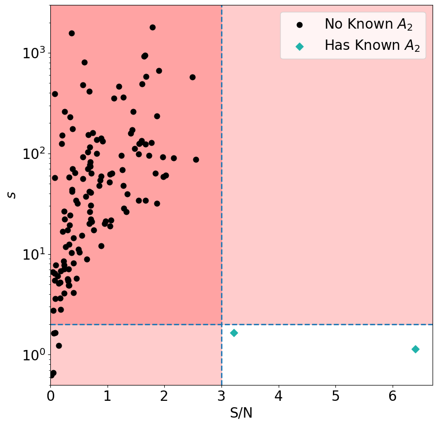
We obtained a total of 6 nights between 2021 April and 2022 February for visible-wavelength follow-up observations with the Semiconductor Technology Associates 10k charge-coupled device (CCD) camera (STACam) on the University of Hawai’i 88 inch (UH88) telescope, observing a total of 134 MBAs (Fig. 1), with 35 having diameters of at most 5 km, as well as, incidentally, one Mars-crosser (Table 1). We selected our targets out of our full thermophysically modeled sample based on what was observable on each night, with higher priority given to targets that had higher-quality thermophysical modeling fits and larger $A_{2}$ estimates. As a point of comparison, we also observed the two NEAs in our thermophysically modeled sample with a previously found Yarkovsky detection: (1685) Toro (JPL) and (1865) Cerberus (JPL).

Our targets were bright ($V\leq 20$ mag in the majority of cases) and generally observed below 1.5 airmass. While we used no filter for the first 3 nights of our observing run, we switched to using the $R$ band for the remaining nights in order to reduce the effects of differential color refraction on the astrometry, which become more significant the further away an observation is from zenith. At airmasses greater than 2, chromatic corrections may be as large as 0.$\arcsec$1 for white light (Tholen & Farnocchia, 2018). The use of any filter that narrows the bandpass will reduce the differential color refraction due to restricting the total wavelength range received by the camera. With the $R$-band in particular, we have the advantage of higher quantum efficiency and better seeing compared with shorter-wavelength filters. The filter also compensated for the somewhat nonuniform color response of the detector, which in turn simplified the flattening process.

Figure 1: Semimajor axes, eccentricities, and inclinations of our 134 MBA targets. The vertical lines in semimajor axis are drawn at the boundaries of the inner ($a<2.0$ au), central ($2.0<a<3.2$ au), and outer ($3.2<a<4.6$ au) main belt regions. Nearly all of our observed MBAs fall within the central main belt region.

We observed each target with a minimum of three dithered exposures to confirm its motion and identity. We set the exposure time to obtain a signal-to-noise ratio (S/N) of at least 10. As nearly all of our targets had apparent magnitudes of $V=20$ mag or brighter, this requirement was achievable with exposures much shorter than a minute for most asteroids. In some cases, however, we discarded exposures due to factors such as issues with telescope tracking inconsistencies, exceptionally poor seeing, or interference between the target and background stars. Additionally, some of our targets were located near the center of the galactic plane, which is home to very dense star fields and thus many potential places for the flux of a background star to abut or completely surround an asteroid. Although we attempted to take observations of this region of the sky, we discarded the observations for a small number of asteroids where we were unable to locate the target within the field.

Ideally, we would have a minimum of two internally consistent observations on different nights to confirm any detection of Yarkovsky drift, but weather conditions precluded second-night observations on several targets. We nonsidereally tracked each target, matching the motion of the target. However, our MBA targets moved slowly enough to keep the background stars as approximate point sources rather than trails in the exposure times we used. The NEAs moved about an order of magnitude faster and thus required a trailed model for the stars, though this had a negligible effect on the accuracy of the astrometry.

Table 1: UH88 Observations

Designation		2021	2021	2021	2021	2021	2022	Predicted $A_{2}$
		Apr 13	May 12	Jun 10	Sep 25	Oct 23	Feb 27	($10^{15}$ au day-2)
767	Bondia	$\cdots$	$\cdots$	$\cdots$	$\cdots$	$\cdots$	✓	$0.07^{+0.01}_{-0.02}$
769	Tatjana	$\cdots$	$\cdots$	$\cdots$	$\cdots$	$\cdots$	✓	$0.16^{+0.03}_{-0.16}$
963	Iduberga	✓	✓	✓	$\cdots$	$\cdots$	$\cdots$	$0.93^{+0.10}_{-0.26}$
1169	Alwine	✓	✓	✓	$\cdots$	$\cdots$	$\cdots$	$-0.91^{+0.64}_{-0.54}$
1415	Malautra	$\cdots$	✓	✓	$\cdots$	$\cdots$	$\cdots$	$0.25^{+0.10}_{-0.16}$

Note. — Observations for each target asteroid separated by date. We observed a total of 134 unique MBAs, as well as one Mars-crosser (2204 Lyyli) and two NEAs (1685 Toro and 1865 Cerberus). Each night consists of at least three dithered exposures per target. Due to the use of multiple shape models in the thermophysical modeling, there is often more than one set of derived thermal properties for an asteroid. The predicted $A_{2}$ reported here uses the thermal inertia, diameter, and albedo derived from the thermophysical modeling fit with the smallest $\chi^{2}$ for that asteroid. Refer to Hung et al. (2022) for more details. The full version of this table can be found in the appendix in Table 4.

We overscan-subtracted, bias-corrected, and flat-fielded the STACam data according to the standard reduction process. We performed the bias correction using a master bias frame generated from a median combination of 15 bias frames taken at the start of each night. We generated the flat field from a median combination of all science images, excluding the images with especially dense star fields. A custom flat field is necessary for targets near the Moon, as the moonlight will create a gradient in the sky background. For the 2 nights where significant moonlight was a concern, we took an average of 12 dithered exposures for any target with a lunar elongation of less than 50$\degree$, which then we median combined to form the custom flat field.

We visually identified the position of the target asteroid in each image, and we matched the reference stars against the Gaia Data Release 2 (DR2; Lindegren et al., 2018) catalog using the astrometric software AstroMagic. The matches made over STACam’s 14.5 arcmin² field of view ranged between around 100 and over 10,000 in the cases of the dense star fields.

We then determined the final positions of the reference stars and target asteroid through a centroiding process, first run using a large aperture to accommodate errors in the AstroMagic pattern matching (e.g., distortions caused by refection) and then again using the optimum aperture, automatically determined by what matched the seeing. In each pass, we fitted a Gaussian distribution to the point-source image profile for each matched reference star and the target asteroid after a background subtraction, where we took the background to be the median value of the pixels in the annulus surrounding the aperture. The least-squares fit was repeated until convergence, which usually happened in about four iterations. Finally, the astrometric fitting was performed over six passes in order to eliminate astrometric and photometric outliers (brought about by, e.g., multiple sources in the same aperture), though all astrometric outliers were usually identified in a single pass. We performed the astrometric fits linearly, as the size of the detector was small enough to ignore higher-order contributions.

The centroiding of the target asteroid was occasionally corrupted due to other sources that were misattributed to the asteroid’s flux. We corrected single bad pixels brought about by cosmic-ray hits or instrument defects by masking. We removed the flux from an abutting background star by a self-subtraction in the image, which involved making a copy of the image. We selected a nearby and slightly brighter isolated star and scaled the flux down in the copied image to match the abutting star. We aligned the abutting star in the original image with the scaled isolated star in the copied image and performed the subtraction. We then performed the centroiding again on the newly isolated asteroid.

We submitted our astrometry to the Minor Planet Center (MPC), with average target asteroid uncertainties on R.A. and decl. positions of 0.$\arcsec$03 and ranging between 0.$\arcsec$01–0.$\arcsec$36. The standard deviation was 0.$\arcsec$03 in R.A. and 0.$\arcsec$02 in decl. Unmodeled sources of error include variations in seeing, transparency, and tracking within the same exposure, but these issues become less of a concern when there is minimal trailing in the background stars, such as in our observations.

4 Orbit Determination

For well-constrained orbits, the orbital deviations caused by the Yarkovsky effect become visible in the data. We computed our orbit solutions with the JPL asteroid and comet orbit determination software. Its methods are described in Farnocchia et al. (2015b). An assumed set of orbital elements and dynamical model will define an initial orbit that is fit to a set of observations. The best fit is determined by the orbit that minimizes the sum of the squares of the residuals, i.e., the differences between the measured and computed sky position for each observation.

In addition to our own observations with UH88, we also used observations from Gaia Data Release 3 (DR3; Tanga et al., 2023), which includes astrometry for over 150,000 solar system objects among its extensive body of data products collected between 2014 July 25 and 2017 May 28. Gaia rotates at a constant rate (Gaia Collaboration et al., 2016), so the transit of a source on the focal plane will end up crossing nine CCD strips. A single transit may thus have up to nine total positions, one for each CCD. The astrometric positions have both per-transit systematic errors and individual random errors. We selected the first position per transit, and the corresponding correlated uncertainty was obtained by adding the systematic and random covariances.

The remaining observations we used come from those reported to the MPC, retrieved on 2023 June 1. The MPC serves as the central database for positional measurements of asteroids and other small bodies. Observation records for MBAs can span time frames over a century. However, most observations obtained from the MPC were reported using a format that did not allow for any communication of astrometric uncertainties. Thus, some assumptions must be made on the uncertainties of each reported observation when computing an orbit, which is handled by way of a weighting scheme. The weights are determined based on statistical analyses of the astrometric errors of past observations, which may be separated by variables such as the historical accuracy of the observing site, reported magnitude, and epoch of observation (e.g., Chesley et al., 2010; Farnocchia et al., 2015a; Vereš et al., 2017). We used the debiasing scheme of Eggl et al. (2020) and the weighting scheme of Vereš et al. (2017) for our orbit determination computations, which are, respectively, the most recent debiasing and weighting schemes available. Outliers were identified and rejected with the scheme described in Carpino et al. (2003).

4.1 Force Model

The gravitational accelerations of the Sun, eight major planets, Pluto, and Moon are accounted for using the JPL planetary and lunar Development Ephemeris DE441 (Park et al., 2021). We also include the gravitational contributions of the 16 most massive perturbers in the main asteroid belt described in the small-body perturber file SB441-N16 (Farnocchia, 2021).

The relativistic contributions of the Sun, planets, and Moon are included through the Einstein–Infeld–Hoffmann equations of motion, which approximate the dynamics of a system of pointlike masses due to mutual gravitational interactions, as well as general relativistic effects. The equations of motion are described in a first-order post-Newtonian expansion as detailed in Einstein et al. (1938), Will (1993), and Moyer (2003).

The Yarkovsky model is the Farnocchia et al. (2013) formulation, which is what is described in §2.

4.2 Determining Valid Detections of $A_{2}$

Plausible detections of $A_{2}$ are defined by the S/N and the indicator parameter $\mathcal{S}$, which is the ratio between the $A_{2}$ derived by the orbit determination and the expected $A_{2}$, typically taken from diameter scaling the $A_{2}$ of a reference asteroid with a reliable Yarkovsky detection (e.g., Farnocchia et al., 2013; Vokrouhlický et al., 2015; Del Vigna et al., 2018). Because we have some knowledge of our asteroid sample’s physical properties thanks to our thermophysical modeling efforts, we can instead use the per-asteroid predicted $A_{2}$ values as described in §3.1.

We consider detection to be valid if it has an S/N of at least 3 with a $\mathcal{S}$ that is close to 1. Cases with $\mathcal{S}\gg 1$ could indicate instances of nongravitational acceleration too strong to be explained by the Yarkovsky effect or, more likely, be spurious detections as a result of a poor orbital fit. Such cases could also imply a much lower bulk density or smaller size for the asteroid than what was assumed. Cases with $\mathcal{S}\ll 1$ would similarly suggest that our predicted $A_{2}$ values are overestimated as a result of inaccuracies in the values used for one or more of the asteroid’s physical parameters, where the Yarkovsky force weakens with larger sizes, higher densities, very high or very low thermal inertia, and obliquities closer to 90$\degree$. However, low-$\mathcal{S}$ cases can still be valid detections of Yarkovsky acceleration and could offer new constraints on the physical properties of the asteroid (Vokrouhlický et al., 2015). We adopt the filtering criteria of Del Vigna et al. (2018) in only accepting detections with both S/N $>3$ and $\mathcal{S}\leq 2$ as valid.

5 Results

With the existing observations, we were unable to find any plausible detections of Yarkovsky acceleration in our observed MBA sample, suggesting that the astrometry was not of sufficient accuracy or observational arc length (Table 2). Every MBA orbit solution produced an $A_{2}$ value at very low S/N, and many values were much larger than predicted.

We did, however, find valid detections with the two NEAs in our sample that already had previously found $A_{2}$ detections in the literature (Fig. 2). The NEAs, (1685) Toro and (1865) Cerberus, show good agreement with the existing estimates. Toro is reported to have an $A_{2}$ of $-3.05\pm 0.46\times 10^{-15}$ au day^-2 in the JPL Small-Body Database. We find an $A_{2}$ of $-2.95\pm 0.46\times 10^{-15}$ au day^-2, which translates to an S/N of 6.4 and is within 1$\sigma$ of the JPL value. Cerberus is reported to have an $A_{2}$ of $-10.22\pm 3.93\times 10^{-15}$ au day^-2 on the JPL Small-Body Database. Our orbit determination gives us an $A_{2}$ of $-11.90\pm 3.69\times 10^{-15}$ au day^-2, corresponding to an S/N of 3.2, which is again within a 1$\sigma$ agreement. The $A_{2}$ value determined can be rather sensitive to the astrometric data set used, coming down to the choice of what observations are included and at what weights, but the close agreement suggests that the differences are minor.

Toro is the only asteroid in our sample with the benefit of existing radar observations, which is partially why its $A_{2}$ detection is of higher S/N than that of Cerberus, which has no radar observations and a slightly shorter observational arc. Cerberus was originally found with a somewhat weak Yarkovsky acceleration signal of 2.1$\sigma$ by Greenberg et al. (2020) using observations between 1971 and 2019. Including our UH88 observations and Gaia DR3, as well as observations from a host of other sites, Cerberus’s observational arc is now 2 yr longer. As a consequence, we have found an improvement to the significance of the Yarkovsky acceleration detection of 1.1$\sigma$, illustrating the importance of having accurate observations for such searches.

Table 2: $A_{2}$ Values from Orbit Determination

Designation		Predicted $A_{2}$	Derived $A_{2}$	S/N	$\mathcal{S}$
		($10^{15}$ au day-2)	($10^{15}$ au day-2)
1685	Toro	$-2.60^{+0.31}_{-0.19}$	$-2.95\pm 0.46$	6.40	1.1
1865	Cerberus	$-7.18^{+0.85}_{-0.57}$	$-11.90\pm 3.69$	3.22	1.7
1773	Rumpelstilz	$0.77^{+0.05}_{-0.09}$	$-67.23\pm 26.41$	2.55	87.2
22092	2000 AQ199	$-0.00^{+0.00}_{-0.23}$	$-132.11\pm 52.99$	2.49	575.1
1430	Somalia	$0.70^{+0.16}_{-0.70}$	$-63.42\pm 29.32$	2.16	90.3

Note. — Solutions for our 134 MBAs, one Mars-crosser (2204 Lyyli), and two NEAs (1685 Toro and 1865 Cerberus). For a detection to be valid, we require both S/N $>3$ and $\mathcal{S}\leq 2$, where $\mathcal{S}$ is the absolute value of the ratio of the derived and predicted $A_{2}$. In cases where the predicted $A_{2}$ was nominally zero, we used the larger error bar value for this calculation instead. Only the NEAs can be considered valid Yarkovsky detections. The remaining MBAs had $A_{2}$ values associated with very low S/N which were often orders of magnitude larger than expected. The full version of this table can be found in the appendix in Table 5.

While our two NEA $A_{2}$ detections fall within 1$\sigma$ agreement with the literature comparisons, we note that this is a much too limited sample size from which to draw any major conclusions. The slight differences between our determined $A_{2}$ values and those in the literature come about mainly due to the differences in the choice of what observations were included in the orbit solution and how the data were weighted. The earliest observations in particular can be highly influential in the orbit solution, as they define the total length of the observational arc, but they are often isolated in time, sometimes separated by several years or decades from the next earliest observations. The accuracy and precision of the earliest observations are also much more suspect compared to modern observations thanks to general technological improvements over time in instruments, cameras, and star catalogs, particularly for observations taken before 1950 (Vereš et al., 2017).

Although weighting schemes can statistically account for the expected accuracy of an observation based on factors such as the observing site or epoch, old data are sparse, which precludes any reliable statistical schemes to correct whatever biases they might have. The star catalog is also often unknown for old observations, which can lead to additional arcseconds of error, as the data cannot be debiased. Ideally, it would be best to manually reweight all suspect observations, but this can be a very time-consuming process with little benefit. It is much more important when working with a plausible new Yarkovsky detection to ensure that an extraordinary result is indeed real, but we have no such cases in our MBA sample.

It is possible to improve the accuracy and precision of archival data by remeasuring against modern star catalogs, as was done for four 1953 precovery observations to confirm a Yarkovsky detection in the orbit of (152563) 1992 BF (Vokrouhlický et al., 2008), but this may not always be feasible. These observations predate the adoption of the CCD in the late 20th century, which replaced photographic plates with a data format that could be electronically stored and processed (Tokunaga, 2014). Observations from photographic plates could only be remeasured if the plates were first digitized, which can be a costly procedure and is dependent on the plates having been preserved in some form over the past several decades. Moreover, nothing can be done about the temporal gaps in the astrometry without coming across more archival data by happenstance, which will be less likely the older the observations are required to be.

Given the low quality of the early observational records, as well as the several variables the Yarkovsky effect depends on, it is difficult to constrain the parameter space with an unsuccessful detection beyond drawing the broadest of conclusions. Let us use the smallest $A_{2}$ uncertainty found among our MBAs as an example. We found an $A_{2}$ uncertainty of $14\times 10^{-15}$ au day^-2 for (1518) Rovaniemi, which means a valid $A_{2}$ detection would be at minimum equal to $42\times 10^{-15}$ au day^-2 in magnitude for an S/N of 3. For this exercise, we will consider our diameter of 8.4 km as robustly determined thanks to the agreement found with the TPM-derived values in Hung et al. (2022) and adopt values for the Bond albedo, thermal inertia, and obliquity in Equation 1 such that we maximize the Yarkovsky acceleration. $A_{2}$ is thus left to vary inversely with the bulk density, where we find that $A_{2}$ only reaches $42\times 10^{-15}$ au day^-2 for a bulk density of 0.080 g cm^-3, too low to be physically plausible and a factor of 34 times smaller than the average S-type bulk density of 2.71 g cm^-3 we adopted for Rovaniemi. Further observations will be necessary for more useful constraints on the parameter space.

Figure 2: $A_{2}$ derived by orbit determination for our sample of 134 MBAs, one Mars-crosser, and two NEAs plotted in terms of the S/N and indicator parameter $\mathcal{S}$. We define the $A_{2}$ to be valid if it has both S/N $>3$ and $\mathcal{S}\leq 2$. All of our MBAs fall outside of this range, while the two NEAs are our only valid detections. Notably, the two NEAs are also the only asteroids in our sample with a previously found $A_{2}$ in the literature.

6 Discussion

6.1 Finding the Minimum Arc Length for Yarkovsky Detectability with Synthetic Observations

The currently available observational data set precluded us from finding any concrete signal of the Yarkovsky effect in the MBAs in our sample, and the lack of detection in turn offered only very poor constraints on the parameter space of the relevant physical properties. We can, however, investigate what observations might be necessary to obtain a Yarkovsky detection using data simulated with the OrbFit software package.

The parameter space for testing synthetic observations is enormous. We could consider the arc length, cadence, precision, and location on Earth of the observations. The orbital properties of the asteroid, such as its semimajor axis and eccentricity, also play an important role, as the difficulty of detecting $A_{2}$ increases with heliocentric distance. In order to simplify our investigation, we consider only the best-case scenario with current technology using a fixed observing strategy with a select few asteroids in order to find a quantified relation between arc length, semimajor axis, and the detectability of $A_{2}$.

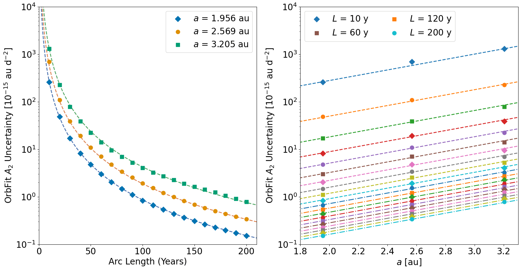
We draw three MBAs from our observed sample to serve as our test cases. Restricting ourselves to low-eccentricity ($e<0.1$) asteroids, we choose the minimum, median, and maximum semimajor axes among them: (45898) 2000 XQ49 at $a=1.955$ au, (50219) 2000 AL237 at $a=2.567$ au, and (13936) 1989 HC at $a=3.201$ au. We use a range of semimajor axes to test the effects of differing angular size, and we use low-eccentricity asteroids to ensure the heliocentric distance is as consistent as possible. We vary the observational arc lengths starting at 1980 January 1 from 10 to 200 yr in steps of 10 yr with a fixed cadence of 50 days between the observations. For each observation, the observer is assumed to be geocentric. The uncertainty on R.A. and decl. is assumed to be 0.$\arcsec$1, a slightly more conservative value than the average uncertainties we found with our UH88 observations.

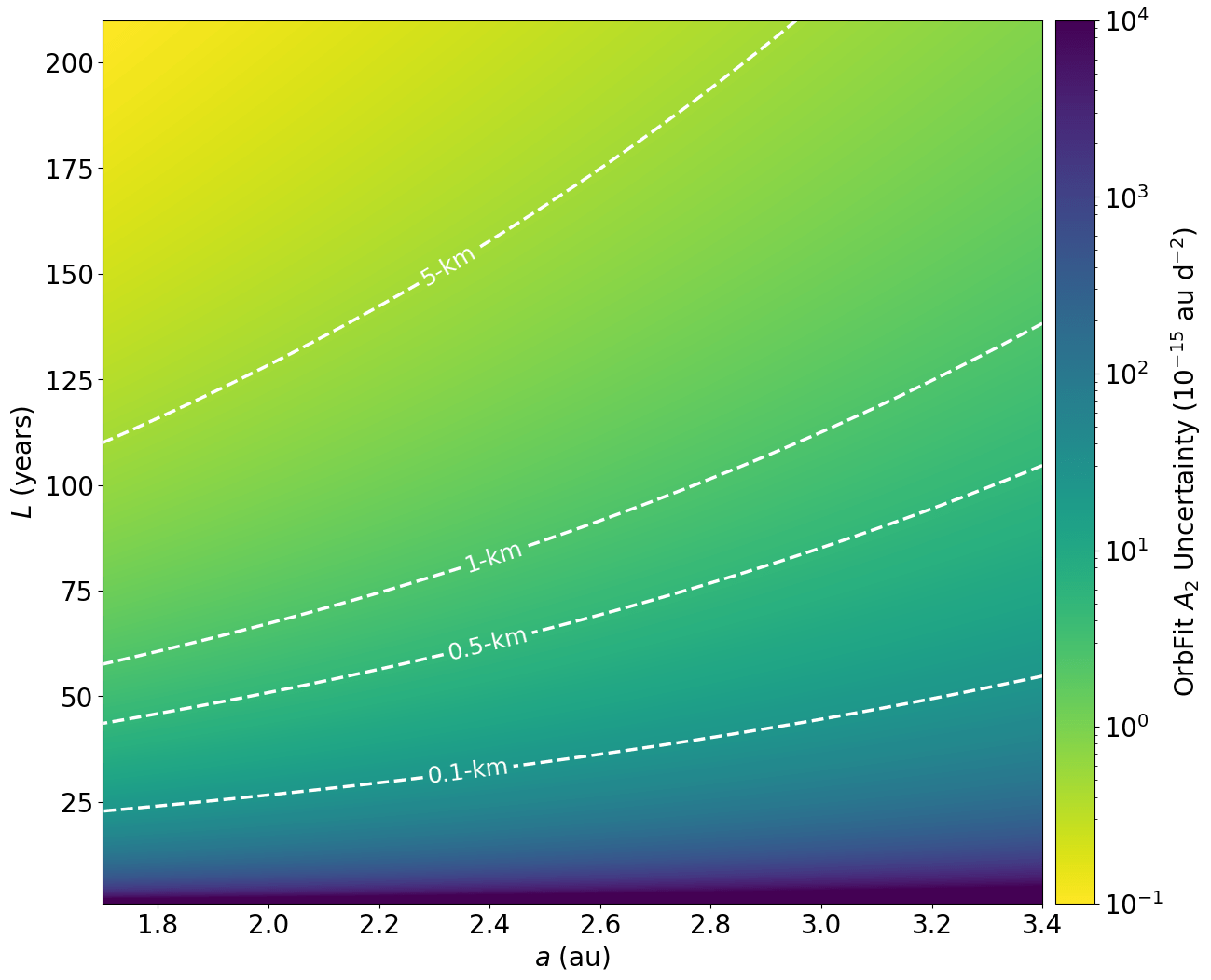
For each set of simulated observations, we used OrbFit to estimate $A_{2}$ and its corresponding uncertainty. The detectability of $A_{2}$ would simply be determined by the S/N, which is the $A_{2}$ value divided by the OrbFit $A_{2}$ uncertainty. Therefore, we can simply express the $A_{2}$ uncertainty as a function of arc length and semimajor axis. The S/N is then obtained by linearly scaling the $A_{2}$ uncertainty to whatever target $A_{2}$ value we choose.

6.2 Detectability Thresholds in Our Observed Sample

If we hold the semimajor axis constant, the relation between arc length $L$ and $A_{2}$ uncertainty $A_{2,unc}$ essentially follows a power law (Fig. 3, left panel). If we hold the arc length constant, the semimajor axis $a$ and $A_{2,unc}$ appear to follow some sort of exponential function (Fig. 3, right panel). We can thus combine the two and fit $A_{2,unc}$ with the two-dimensional function

$$f(L,a)=k10^{c(a-2.6)}L^{\alpha}$$ (7)

where $k$, $c$, and $\alpha$ are our fitting coefficients. We use the minimize routine with the Nelder–Mead method (Nelder & Mead, 1965) in the Python library SciPy to minimize the sum of the residuals $r$, which are given by

$$\sum_{i}r_{i}^{2}=\sum_{i}\left(1-f(L_{i},a_{i})/A_{2,unc_{i}}\right)^{2}$$ (8)

We minimize the relative error on $A_{2,unc}$ rather than the absolute in order to avoid biasing the fit toward larger values of the $A_{2}$ uncertainty, which would consequently lead us to better fit shorter observational arcs than longer arcs. We find best-fit values of $k=1.852\times 10^{5}$, $c=0.556$, and $\alpha=-2.488$. We stress for the reader’s consideration that our fit here is only a proxy for the detectability of the Yarkovsky effect in the main belt.

Figure 3: The $A_{2}$ uncertainty as a function of observational arc length $L$ and asteroid semimajor axis $a$. With the semimajor axis fixed in the left panel, the arc length $L$ and $A_{2}$ uncertainty $A_{2,unc}$ follow a power law. With the arc length fixed in the right panel, $a$ and $A_{2,unc}$ follow an exponential function. Note that the $A_{2}$ uncertainty decreases as the arc length increases from 10 to 200 yr in 10 yr steps, but we only include four arc lengths in the legend for the purpose of brevity. The fitted lines are plotted from our two-dimensional fit, $f(L,a)=k10^{c(a-2.6)}L^{\alpha}$, where the values of the coefficients are $k=1.852\times 10^{5}$, $c=0.556$, and $\alpha=-2.488$.

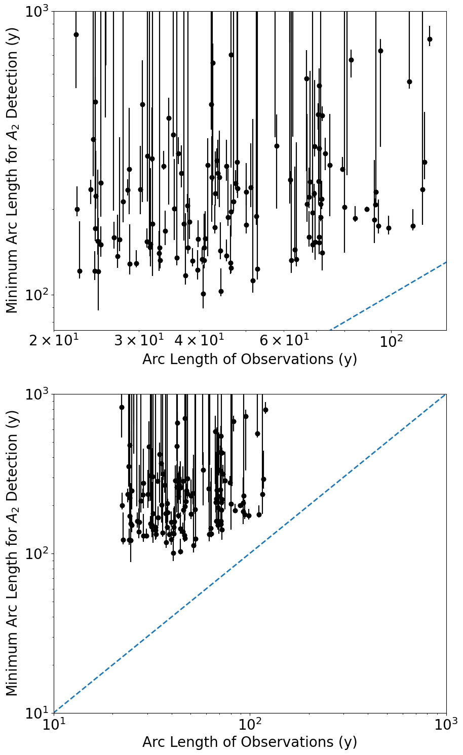
The semimajor axis is a known quantity for every asteroid in our observed sample. If we define the threshold for detectability to be S/N = 3, then the $A_{2}$ uncertainty must be a third of the target $A_{2}$ value. With this in mind, we can thus translate the predicted $A_{2}$ values of our sample into minimum arc lengths for detectability with Equation 7 (Table 3). If we compare our minimum arc lengths for Yarkovsky detectability to the arc lengths of the existing observations for our observed sample of MBAs, we see that no asteroids come close to meeting the threshold (Fig. 4). Even if any had met the threshold, it is unlikely that we would have been able to find a successful Yarkovsky detection. The synthetic observations were modeled after the best-case scenario under modern-day standards, with a regular cadence and much higher levels of precision than were accessible a century ago (Vereš et al., 2017). Observations of lower precision will necessitate longer arc lengths for Yarkovsky detection to be possible for a given $A_{2}$ value. While (767) Bondia, for example, has the longest observational arc in our sample, with its earliest observations in 1902, there are multiple years-long gaps in its pre-1956 record, and many observations are only to arcminute precision. Finally, it is also important to note that this discussion is in part predicated on the accuracy of our predicted $A_{2}$ values, which can vary between asteroids due to differences in data quality. The predicted $A_{2}$ values were estimated from parameters derived through thermophysical modeling (see §3.1), which becomes less reliable when applied to cruder shape models (Hung et al., 2022).

Table 3: Minimum Arc Lengths Needed for Yarkovsky Detection

Designation		$a$	$e$	Predicted $A_{2}$	Min. $L$	Current $L$
		(au)		($10^{15}$ au day-2)	(yr)	(yr)
767	Bondia	3.119	0.1829	$0.07^{+0.01}_{-0.02}$	751–888	120
769	Tatjana	3.166	0.1870	$0.16^{+0.03}_{-0.16}$	532+	109
963	Iduberga	2.248	0.1378	$0.93^{+0.10}_{-0.26}$	168–200	111
1169	Alwine	2.319	0.1549	$-0.91^{+0.64}_{-0.54}$	152–299	92
1415	Malautra	2.223	0.0874	$0.25^{+0.10}_{-0.16}$	255–441	117

Note. — Minimum observational arc lengths $L$ needed to detect a predicted $A_{2}$ value at S/N = 3 for our sample of 134 observed MBAs and one Mars-crosser (2204 Lyyli), calculated as described in §6.2. The semimajor axis $a$ and eccentricity $e$ are taken from the JPL Small-Body Database. The predicted $A_{2}$ values are estimated from TPM-derived parameters as described in §3.1. The current arc lengths are the total time span of the existing observations for each asteroid, last retrieved on 2023 January 1. The minimum arc length spans cover the $1\sigma$ range in the predicted $A_{2}$ values. In instances where the predicted $A_{2}$ reaches zero, the minimum arc length is essentially infinite; thus, we only report a lower bound for such asteroids. The full version of this table can be found in the appendix in Table 6.

6.3 Detectability Thresholds for Undiscovered MBAs

Figure 4: We compare the observational arc lengths of our observed sample of MBAs with the minimum arc lengths needed for a Yarkovsky detection. The dashed line shows where the two axes are equal. The error bars on the minimum arc lengths are based on the error bars on the predicted $A_{2}$ values derived from our TPM fitting as described in §3.1. They are best taken strictly as lower limits due to the caveats described in §6.2. None of our observed asteroids have long enough arcs to meet the threshold for Yarkovsky detection.

The difficulty in detecting the Yarkovsky effect in the main belt is in part due to the sizes of known MBAs. An MBA of the same size as an NEA would be more difficult to detect due to the drop-off in apparent magnitude with heliocentric distance; thus, many fewer subkilometer MBAs are known relative to NEAs as a result of observational bias. However, we can expect asteroid discovery capabilities to dramatically improve in the near future with upcoming surveys such as the Vera Rubin Observatory Legacy Survey of Space and Time (LSST; Ivezić et al., 2019), expected in 2024, which will be able to probe fainter magnitudes. LSST will have an 8.4 m primary mirror with a 9.6 deg² field of view and is expected to be capable of detecting asteroids with diameters in the range of 100 m at main belt distances.

Previous Yarkovsky studies have used a relation scaling with the most reliable Yarkovsky detection to obtain an expected value for $A_{2}$ in cases where the physical characterization of an asteroid is unknown (e.g., Farnocchia et al., 2013; Del Vigna et al., 2018). The Yarkovsky effect is inversely proportional to the asteroid diameter, so the scaling relation is of the form

$$A_{2,\mathrm{exp}}=A_{2,\mathrm{ref}}\frac{D_{\mathrm{ref}}}{D}$$ (9)

where $A_{2,\mathrm{exp}}$ is the expected $A_{2}$ for an asteroid of diameter $D$ scaled with the corresponding values of a reference asteroid. In order to keep the parameter space as simple as possible, we assume all other parameters that affect the Yarkovsky acceleration, such as the bulk density, obliquity, and albedo, to be the same as the reference asteroid. Currently, the most reliable detection is that of (101955) Bennu. Bennu was visited by the sample return mission OSIRIS-REx (Lauretta et al., 2017) from late 2018 to 2020, where the addition of the spacecraft’s tracking data and physical characterization helped refine Bennu’s Yarkovsky detection down to 0.07% precision (Farnocchia et al., 2021).

Bennu has an estimated semimajor axis drift rate of $\left\langle da/dt\right\rangle=-284.6\pm 0.2$ m y^-1 (Farnocchia et al., 2021) and an equivalent diameter of 0.482 km (Daly et al., 2020). Using equation 5 in Farnocchia et al. (2013) with $a_{\mathrm{Bennu}}=1.126$ au, $e_{\mathrm{Bennu}}=0.204$, and $n_{\mathrm{Bennu}}=0.824$ deg d^-1 and assuming $d=2$, this translates to an $A_{2,\mathrm{Bennu}}$ of $-45.57\pm 0.03\times 10^{-15}$ au day^-2.

Figure 5: The diameters of the nearly 2000 MBAs thermophysically modeled in Hung et al. (2022) plotted against the absolute values of their predicted $A_{2}$, which was estimated from their derived parameters. The scaling relation from Equation 9 using the values of Bennu produces consistently higher expected $A_{2}$ values than predicted, but we see better agreement if we reduce the relation by a factor of 3.

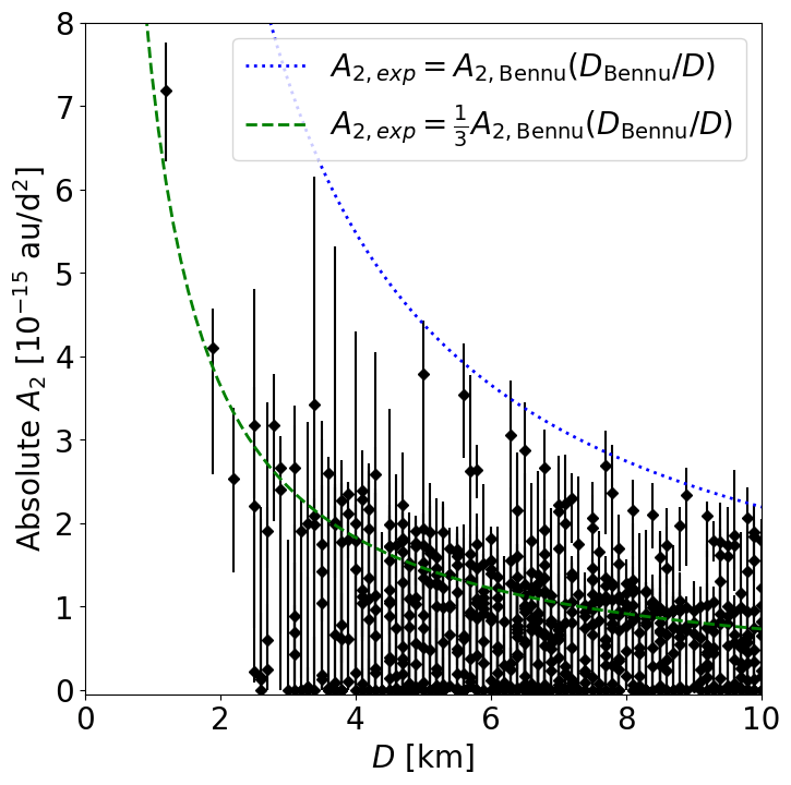
It is important to note, however, that Bennu as an NEA may not necessarily be reflective of the general population of MBAs. Even among NEAs, Bennu is notable for its extreme obliquity and low bulk density ($\sim$1 g cm^-3; Farnocchia et al., 2021), which both maximize the Yarkovsky acceleration. Using Bennu as our reference asteroid consistently yields expected $A_{2}$ values that are higher than the $A_{2}$ values we estimated with our TPM-derived parameters. We can, however, find better agreement if we simply apply a factor of one-third to the scaling relation (Fig. 5). While this method of estimation is very crude, the exact numbers are not overly important, as we are only interested in using the scaling relation to determine rough Yarkovsky detectability thresholds for undiscovered asteroids.

Using the modified scaling relation, we expect a 100 m MBA to have an $A_{2,\mathrm{exp}}$ of $73\times 10^{-15}$ au day^-2 and a 1-km MBA to have an $A_{2,\mathrm{exp}}$ of $7.3\times 10^{-15}$ au day^-2. With Equation 7, we can find the minimum arc length to detect the Yarkovsky effect as a function of semimajor axis. While with current technology, it would only become possible to detect a Yarkovsky drift in the central main belt region in about 80 yr for a 1 km MBA, detection is dramatically easier for 100 m MBAs, where it would take about 30 yr (Fig. 6). So long as we can find such small MBAs and maintain consistent high-quality astrometry, a Yarkovsky detection in the main belt is achievable within a reasonable time frame.

Figure 6: Equation 7 is represented here as a three-dimensional plot, with the $A_{2}$ uncertainty as a function of the semimajor axis $a$ and observational arc length $L$. Overplotted are contour lines for the minimum arc length for the Yarkovsky effect to become detectable as a function of $a$ for MBAs of 0.1, 0.5, 1, and 5 km in diameter, where their $A_{2}$ values are estimated from the diameter scaling relation described in Figure 5.

7 Conclusions and Future Prospects

Although there are hundreds of reported cases among the NEA population, the Yarkovsky effect has never been detected in individual MBAs, and that fact remains true with our attempts in this work. Using our sample of over a thousand thermophysically modeled MBAs, we were able to identify among them the most promising candidates for direct Yarkovsky detection based on their predicted $A_{2}$ values. We observed a subset of these candidates with the UH88, and we attempted to look for direct signs of Yarkovsky acceleration with the JPL asteroid and comet orbit determination software, where our observational data consisted of data from our UH88 observations, Gaia DR3, and archival astrometry reported at the MPC.

The majority of MBAs in our sample have archival data spanning many decades, with a few having total arc lengths of longer than a century. Long observational arcs provide greater constraints for the orbit determination and thus are advantageous to have when attempting to detect Yarkovsky-induced orbital drift. However, the historical data from up through the mid-20th century are often of much cruder precision and lower quality in comparison to astrometric positions from the past few decades (Vereš et al., 2017) thanks to technological advancements across telescopes and detectors Tokunaga (see e.g., the review by 2014) as well as larger and more accurate star catalogs (e.g., Anders et al., 2022; Gaia Collaboration et al., 2023). With the release of Gaia DR3 (Tanga et al., 2023), we have hundreds of yet-unused highly accurate astrometric positions for many of the asteroids in our sample. As expected, the improvements to the orbit solutions provided by these observations were largely marginal and not sufficient to produce a plausible Yarkovsky detection among any of our MBAs. The Gaia mission was only launched in 2013, in the modern era where observations of MBAs from ground-based observatories are plentiful and a regular occurrence.

We showed that the existing observations are not of sufficiently high accuracy or precision to constrain the Yarkovsky effect. Using synthetic observations assuming a certain value for $A_{2}$, we found the minimum observational arc length required to detect the Yarkovsky effect given an expected $A_{2}$ and semimajor axis. It should be stressed, however, that this minimum is under the best-case conditions, where the asteroid is regularly observed throughout the whole arc and at a level of accuracy (0.$\arcsec$1) that is generally high even for modern-day astrometry (Vereš et al., 2017). Note that we also do not take into consideration the viability of an individual observation (e.g., limitations on magnitude or solar elongation), but main belt orbits are easily accessible for observations on a yearly basis, and the interval between observations is not significant as long as it is short compared with the total arc length. Searches for Yarkovsky acceleration have sometimes found detections that are strongly dependent on a few observations that are separated by a long time interval from the rest of the data set (e.g., Farnocchia et al., 2013; Del Vigna et al., 2018). Remeasuring these isolated observations against modern star catalogs could confirm whether or not the Yarkovsky acceleration signal is real, as was done for the four 1953 precovery observations of (152563) 1992 BF (Vokrouhlický et al., 2008), but the data may not necessarily have been preserved to make such remeasurements possible.

Even if we were to find a valid Yarkovsky detection in the main belt, it cannot be considered reliable without the full consideration of the effects of the completeness of the perturbing asteroids and the uncertainties in their masses. While NEAs are relatively isolated, MBAs will spend more time in closer proximity to other asteroids in the main belt. Because of this, MBAs may be more sensitive to the gravitational perturbations of other asteroids than NEAs. The effects of perturbing asteroids may be inaccurately modeled, as methods for asteroid mass determination are limited, and derived masses are often associated with large uncertainties (e.g., Carry, 2012). The most precise mass estimates come from spacecraft flybys of asteroids, but such missions are incredibly costly and thus very few in number (e.g., Pätzold et al., 2011; Konopliv et al., 2014; Lauretta et al., 2017). Multiple-asteroid systems provide the next most reliable method for mass determination through Kepler’s third law and knowledge of the satellites’ orbits around the primary asteroid (e.g., Fang et al., 2011; Rojo & Margot, 2011; Yang et al., 2020; Drummond et al., 2021; Vernazza et al., 2021). The most common mass estimates have come from close encounters with other asteroids (e.g., Michalak, 2000, 2001; Kovačević, 2012; Baer & Chesley, 2017; Li et al., 2019) or Mars (e.g., Pitjeva, 2001; Mouret et al., 2009), but the accuracy can be very crude for smaller asteroids (e.g., Zielenbach, 2011; Carry, 2012). Mass estimates are only available for a few hundred asteroids (Carry, 2012); thus, it is possible that significant perturbers are not included in the dynamical models at all. If such an unknown perturber happened to be on an orbit trailing or leading a target asteroid, its gravitational contribution might end up mimicking or masking the effects of Yarkovsky acceleration. The perturber sensitivity problem was explored in depth with the Yarkovsky detection of Bennu (Farnocchia et al., 2021), where the model included a total of 343 asteroid perturbers with their mass uncertainties, and the convergence of the orbital solution indicated that the perturber set was sufficient.

The best path forward to confirm the Yarkovsky effect in the main belt is simply more time, but the future is promising. Many MBAs are bright enough to be easily seen by survey telescopes such as the Panoramic Survey Telescope and Rapid Response System (Pan-STARRS1) telescope (Chambers et al., 2016) and the Catalina Sky Survey. These surveys discover thousands of new NEAs every year by scanning the entire night sky on a routine basis and at the same time obtain many incidental follow-up observations of MBAs, which have orbits ensuring that they will be observable at regular, roughly yearly intervals. Upcoming near-future surveys such as LSST (Ivezić et al., 2019) are especially promising, as they will be capable of reaching deeper magnitudes and discovering much smaller MBAs where the Yarkovsky force is stronger and more easily detected. With our synthetic observations, we have shown that the Yarkovsky acceleration should be detectable in 100 m MBAs within a couple of decades. LSST in particular will be especially fruitful for asteroid discovery and follow-up, as it will operate in the Southern Hemisphere, which has traditionally seen much less observational coverage than the Northern Hemisphere.

Although we have no direct confirmation of Yarkovsky-induced orbital drift on any individual asteroid in the main belt as of yet, detection is in a sense inevitable as the body of high-quality astrometry grows. There are no benchmark tests to verify the accuracy of thermophysically derived parameters, and ground-truth information is highly limited, restricted to spacecraft missions that are only feasible for a very small number of asteroids. However, a successful detection of Yarkovsky acceleration could serve as a means of constraining the physical properties of an asteroid that are independent of its thermal data and the limitations of the thermophysical models. The first MBA Yarkovsky detection may end up occurring with a yet-undiscovered asteroid, but thermal data of asteroids will only grow more plentiful with upcoming space-based surveys like the Near-Earth Object Surveyor. The detection of Bennu’s Yarkovsky acceleration combined with its thermophysically derived parameters made it possible to estimate its bulk density (Chesley et al., 2014), a value that was later confirmed by spacecraft tracking measurements (Scheeres et al., 2019). Of course, these are only hypothetical scenarios for MBAs for now, but in time, we will have a better understanding of the makeup of the largest group of asteroids in the solar system.

8 Appendix

Table 4: UH88 Observations

Designation		2021	2021	2021	2021	2021	2022	Predicted $A_{2}$
		Apr 13	May 12	Jun 10	Sep 25	Oct 23	Feb 27	($10^{15}$ au day-2)
767	Bondia	$\cdots$	$\cdots$	$\cdots$	$\cdots$	$\cdots$	✓	$0.07^{+0.01}_{-0.02}$
769	Tatjana	$\cdots$	$\cdots$	$\cdots$	$\cdots$	$\cdots$	✓	$0.16^{+0.03}_{-0.16}$
963	Iduberga	✓	✓	✓	$\cdots$	$\cdots$	$\cdots$	$0.93^{+0.10}_{-0.26}$
1169	Alwine	✓	✓	✓	$\cdots$	$\cdots$	$\cdots$	$-0.91^{+0.64}_{-0.54}$
1415	Malautra	$\cdots$	✓	✓	$\cdots$	$\cdots$	$\cdots$	$0.25^{+0.10}_{-0.16}$
1430	Somalia	✓	✓	$\cdots$	$\cdots$	$\cdots$	$\cdots$	$0.70^{+0.16}_{-0.70}$
1518	Rovaniemi	$\cdots$	$\cdots$	✓	$\cdots$	$\cdots$	$\cdots$	$0.91^{+0.16}_{-0.37}$
1652	Herge	$\cdots$	$\cdots$	✓	$\cdots$	$\cdots$	$\cdots$	$0.67^{+0.02}_{-0.04}$
1685	Toro	✓	✓	✓	$\cdots$	$\cdots$	$\cdots$	$-2.60^{+0.31}_{-0.19}$
1704	Wachmann	$\cdots$	✓	✓	$\cdots$	$\cdots$	$\cdots$	$0.94^{+0.14}_{-0.20}$
1772	Gagarin	$\cdots$	✓	$\cdots$	$\cdots$	$\cdots$	$\cdots$	$0.05^{+0.02}_{-0.01}$
1773	Rumpelstilz	✓	✓	✓	$\cdots$	$\cdots$	$\cdots$	$0.77^{+0.05}_{-0.09}$
1865	Cerberus	$\cdots$	$\cdots$	$\cdots$	✓	✓	$\cdots$	$-7.18^{+0.85}_{-0.57}$
2204	Lyyli	$\cdots$	$\cdots$	$\cdots$	$\cdots$	$\cdots$	✓	$-0.46^{+0.10}_{-0.02}$
2493	Elmer	✓	✓	$\cdots$	$\cdots$	$\cdots$	$\cdots$	$-0.77^{+0.69}_{-0.23}$
2818	Juvenalis	$\cdots$	$\cdots$	$\cdots$	✓	$\cdots$	$\cdots$	$-2.22^{+2.22}_{-0.62}$
2840	Kallavesi	✓	✓	✓	$\cdots$	$\cdots$	$\cdots$	$0.00^{+0.41}_{-0.00}$
2874	Jim Young	✓	✓	✓	$\cdots$	$\cdots$	$\cdots$	$0.71^{+0.65}_{-0.71}$
3121	Tamines	✓	✓	✓	$\cdots$	$\cdots$	$\cdots$	$0.27^{+0.48}_{-0.17}$
3376	Armandhammer	✓	✓	✓	$\cdots$	$\cdots$	$\cdots$	$0.11^{+0.04}_{-0.02}$
3383	Koyama	✓	✓	✓	$\cdots$	$\cdots$	$\cdots$	$0.81^{+0.18}_{-0.25}$
3510	Veeder	✓	✓	✓	$\cdots$	$\cdots$	$\cdots$	$0.71^{+0.06}_{-0.13}$
3556	Lixiaohua	$\cdots$	$\cdots$	$\cdots$	$\cdots$	$\cdots$	✓	$-0.00^{+0.00}_{-0.51}$
3722	Urata	$\cdots$	$\cdots$	$\cdots$	$\cdots$	$\cdots$	✓	$-0.03^{+0.01}_{-0.16}$
4005	Dyagilev	✓	✓	✓	$\cdots$	$\cdots$	$\cdots$	$0.28^{+0.11}_{-0.08}$
4088	Baggesen	$\cdots$	✓	✓	$\cdots$	$\cdots$	$\cdots$	$0.61^{+0.19}_{-0.27}$
4113	Rascana	$\cdots$	$\cdots$	✓	$\cdots$	$\cdots$	$\cdots$	$-0.19^{+0.09}_{-0.48}$
4285	Hulkower	$\cdots$	$\cdots$	$\cdots$	$\cdots$	$\cdots$	✓	$-1.28^{+1.28}_{-0.24}$
4323	Hortulus	✓	✓	✓	$\cdots$	$\cdots$	$\cdots$	$1.31^{+0.34}_{-0.56}$
4399	Ashizuri	$\cdots$	✓	✓	$\cdots$	$\cdots$	$\cdots$	$-0.30^{+0.17}_{-0.57}$
4515	Khrennikov	$\cdots$	✓	✓	$\cdots$	$\cdots$	$\cdots$	$-1.60^{+1.03}_{-0.70}$
4912	Emilhaury	✓	✓	✓	$\cdots$	$\cdots$	$\cdots$	$-1.46^{+1.14}_{-0.25}$
4928	Vermeer	✓	✓	$\cdots$	$\cdots$	$\cdots$	$\cdots$	$-1.99^{+0.64}_{-0.43}$
4959	Niinoama	$\cdots$	$\cdots$	$\cdots$	$\cdots$	$\cdots$	✓	$-0.32^{+0.05}_{-0.04}$
5589	De Meis	✓	✓	$\cdots$	$\cdots$	$\cdots$	$\cdots$	$-1.15^{+0.96}_{-0.49}$
5635	Cole	✓	✓	$\cdots$	$\cdots$	$\cdots$	$\cdots$	$0.32^{+1.73}_{-0.14}$
5889	Mickiewicz	$\cdots$	$\cdots$	$\cdots$	$\cdots$	$\cdots$	✓	$-0.70^{+0.15}_{-0.10}$
5958	Barrande	$\cdots$	✓	$\cdots$	$\cdots$	$\cdots$	$\cdots$	$-0.05^{+0.02}_{-0.30}$
6499	Michiko	$\cdots$	✓	$\cdots$	$\cdots$	$\cdots$	$\cdots$	$-0.74^{+0.49}_{-0.43}$
6581	Sobers	$\cdots$	$\cdots$	$\cdots$	$\cdots$	$\cdots$	✓	$-1.99^{+1.21}_{-0.35}$
6607	Matsushima	$\cdots$	$\cdots$	$\cdots$	$\cdots$	$\cdots$	✓	$-0.71^{+0.71}_{-0.15}$
6714	Montreal	✓	✓	✓	$\cdots$	$\cdots$	$\cdots$	$0.05^{+0.51}_{-0.02}$
6755	Solov’yanenko	$\cdots$	✓	✓	$\cdots$	$\cdots$	$\cdots$	$1.17^{+0.22}_{-0.69}$
6915	(1992 HH)	✓	✓	✓	$\cdots$	$\cdots$	$\cdots$	$-0.51^{+0.25}_{-0.35}$
7196	Baroni	$\cdots$	$\cdots$	$\cdots$	✓	✓	$\cdots$	$-2.17^{+1.15}_{-0.54}$
7517	Alisondoane	✓	✓	✓	$\cdots$	$\cdots$	$\cdots$	$1.04^{+0.07}_{-0.22}$
7684	Marioferrero	✓	✓	✓	$\cdots$	$\cdots$	$\cdots$	$1.06^{+0.27}_{-0.47}$
8359	(1989 WD)	$\cdots$	$\cdots$	✓	$\cdots$	$\cdots$	$\cdots$	$-1.85^{+0.67}_{-0.79}$
9008	Bohsternberk	$\cdots$	$\cdots$	✓	$\cdots$	$\cdots$	$\cdots$	$-1.73^{+0.40}_{-0.20}$
9158	Plate	✓	✓	$\cdots$	$\cdots$	$\cdots$	$\cdots$	$-1.55^{+0.76}_{-0.44}$
9173	Viola Castello	$\cdots$	✓	$\cdots$	$\cdots$	$\cdots$	$\cdots$	$-1.15^{+1.15}_{-0.24}$
9234	Matsumototaku	$\cdots$	$\cdots$	$\cdots$	✓	✓	$\cdots$	$-2.67^{+2.56}_{-0.74}$
9274	Amylovell	$\cdots$	$\cdots$	$\cdots$	$\cdots$	✓	$\cdots$	$-2.63^{+1.28}_{-1.14}$
9566	Rykhlova	$\cdots$	$\cdots$	$\cdots$	$\cdots$	✓	$\cdots$	$-1.97^{+0.55}_{-0.23}$
9582	(1990 EL7)	$\cdots$	$\cdots$	$\cdots$	$\cdots$	✓	$\cdots$	$-2.00^{+2.00}_{-0.48}$
10166	Takarajima	✓	✓	✓	$\cdots$	$\cdots$	$\cdots$	$-0.00^{+0.00}_{-2.48}$
10338	(1991 RB11)	$\cdots$	$\cdots$	$\cdots$	$\cdots$	$\cdots$	✓	$-0.09^{+0.08}_{-0.78}$
10406	(1997 WZ29)	$\cdots$	$\cdots$	$\cdots$	$\cdots$	$\cdots$	✓	$-1.35^{+0.32}_{-0.17}$
10456	Anechka	✓	✓	✓	$\cdots$	$\cdots$	$\cdots$	$1.82^{+0.36}_{-0.79}$
10656	Albrecht	✓	✓	$\cdots$	$\cdots$	$\cdots$	$\cdots$	$-0.61^{+0.45}_{-0.14}$
11676	(1998 CQ2)	$\cdots$	$\cdots$	$\cdots$	✓	✓	$\cdots$	$-2.64^{+0.34}_{-0.30}$
11823	Christen	$\cdots$	$\cdots$	$\cdots$	$\cdots$	$\cdots$	✓	$1.77^{+0.31}_{-1.44}$
11889	(1991 AH2)	✓	✓	✓	$\cdots$	$\cdots$	$\cdots$	$0.46^{+0.04}_{-0.30}$
12097	(1998 HG121)	$\cdots$	✓	✓	$\cdots$	$\cdots$	$\cdots$	$1.04^{+0.44}_{-0.40}$
12374	Rakhat	✓	✓	$\cdots$	$\cdots$	$\cdots$	$\cdots$	$1.72^{+0.36}_{-0.70}$
12555	(1998 QP47)	✓	✓	✓	$\cdots$	$\cdots$	$\cdots$	$-0.58^{+0.58}_{-0.51}$
12617	Angelusilesius	$\cdots$	$\cdots$	$\cdots$	$\cdots$	$\cdots$	✓	$-0.00^{+0.00}_{-0.99}$
12690	Kochimiraikagaku	$\cdots$	$\cdots$	$\cdots$	$\cdots$	$\cdots$	✓	$-0.21^{+0.21}_{-0.14}$
12705	(1990 TJ)	✓	✓	✓	$\cdots$	$\cdots$	$\cdots$	$-0.51^{+0.31}_{-0.41}$
12883	(1998 QY32)	✓	✓	✓	$\cdots$	$\cdots$	$\cdots$	$-0.00^{+0.00}_{-0.64}$
12926	Brianmason	$\cdots$	$\cdots$	$\cdots$	✓	✓	$\cdots$	$2.06^{+0.37}_{-0.52}$
13007	(1984 AU)	✓	✓	✓	$\cdots$	$\cdots$	$\cdots$	$-0.65^{+0.65}_{-0.67}$
13019	(1988 NW)	✓	✓	$\cdots$	$\cdots$	$\cdots$	$\cdots$	$0.71^{+0.35}_{-0.42}$
13059	Ducuroir	✓	✓	✓	$\cdots$	$\cdots$	$\cdots$	$1.89^{+0.34}_{-0.60}$
13446	Almarkim	$\cdots$	$\cdots$	$\cdots$	$\cdots$	$\cdots$	✓	$0.00^{+0.07}_{-0.00}$
13883	(7066 P-L)	$\cdots$	$\cdots$	$\cdots$	$\cdots$	$\cdots$	✓	$1.01^{+0.09}_{-0.16}$
13925	(1986 QS3)	✓	✓	✓	$\cdots$	$\cdots$	$\cdots$	$-0.57^{+0.16}_{-0.14}$
13936	(1989 HC)	$\cdots$	$\cdots$	$\cdots$	$\cdots$	$\cdots$	✓	$0.95^{+0.07}_{-0.25}$
13948	(1990 QB6)	$\cdots$	$\cdots$	$\cdots$	$\cdots$	$\cdots$	✓	$0.43^{+0.63}_{-0.24}$
14031	Rozyo	✓	✓	✓	$\cdots$	$\cdots$	$\cdots$	$-0.88^{+0.88}_{-0.46}$
14257	(2000 AR97)	$\cdots$	$\cdots$	✓	$\cdots$	$\cdots$	$\cdots$	$0.62^{+0.94}_{-0.62}$
15920	(1997 UB25)	$\cdots$	$\cdots$	$\cdots$	$\cdots$	✓	$\cdots$	$-2.40^{+1.72}_{-0.49}$
17431	Sainte-Colombe	$\cdots$	$\cdots$	$\cdots$	✓	✓	$\cdots$	$2.12^{+0.38}_{-0.53}$
18591	(1997 YT11)	$\cdots$	$\cdots$	✓	$\cdots$	$\cdots$	$\cdots$	$0.48^{+0.72}_{-0.34}$
18997	Mizrahi	$\cdots$	$\cdots$	$\cdots$	✓	✓	$\cdots$	$-2.66^{+2.66}_{-0.46}$
19136	Strassmann	$\cdots$	$\cdots$	$\cdots$	✓	✓	$\cdots$	$-2.27^{+2.27}_{-0.48}$
19876	(7637 P-L)	$\cdots$	$\cdots$	$\cdots$	✓	✓	$\cdots$	$2.09^{+0.32}_{-1.89}$
20179	(1996 XX31)	$\cdots$	$\cdots$	$\cdots$	✓	✓	$\cdots$	$-2.36^{+1.30}_{-0.58}$
20498	(1999 RT1)	$\cdots$	$\cdots$	$\cdots$	$\cdots$	$\cdots$	✓	$0.00^{+1.08}_{-0.00}$
20515	(1999 RO34)	$\cdots$	$\cdots$	$\cdots$	$\cdots$	$\cdots$	✓	$0.91^{+0.29}_{-0.39}$
20557	Davidkulka	✓	✓	✓	$\cdots$	$\cdots$	$\cdots$	$1.42^{+0.29}_{-0.60}$
20681	(1999 VH10)	$\cdots$	✓	✓	$\cdots$	$\cdots$	$\cdots$	$0.99^{+0.27}_{-0.56}$
21041	(1990 QO1)	$\cdots$	$\cdots$	$\cdots$	✓	✓	$\cdots$	$-2.06^{+1.29}_{-0.39}$
21842	(1999 TH102)	$\cdots$	$\cdots$	$\cdots$	$\cdots$	$\cdots$	✓	$-0.44^{+0.44}_{-0.25}$
22092	(2000 AQ199)	$\cdots$	$\cdots$	$\cdots$	$\cdots$	$\cdots$	✓	$-0.00^{+0.00}_{-0.23}$
24181	(1999 XN8)	✓	✓	✓	$\cdots$	$\cdots$	$\cdots$	$-1.38^{+1.38}_{-0.55}$
25887	(2000 SU308)	$\cdots$	$\cdots$	$\cdots$	✓	✓	$\cdots$	$2.34^{+0.32}_{-0.86}$
26176	(1996 GD2)	$\cdots$	$\cdots$	$\cdots$	✓	✓	$\cdots$	$-2.22^{+0.59}_{-0.58}$
26520	(2000 CQ75)	$\cdots$	$\cdots$	$\cdots$	$\cdots$	$\cdots$	✓	$1.04^{+0.34}_{-1.04}$
27259	(1999 XS136)	✓	✓	$\cdots$	$\cdots$	$\cdots$	$\cdots$	$1.18^{+0.11}_{-0.14}$
28709	(2000 GY96)	$\cdots$	$\cdots$	$\cdots$	$\cdots$	$\cdots$	✓	$-1.41^{+0.28}_{-0.15}$
28736	(2000 GE133)	$\cdots$	$\cdots$	$\cdots$	✓	✓	$\cdots$	$-2.09^{+0.49}_{-0.18}$
30072	(2000 EP93)	✓	✓	$\cdots$	$\cdots$	$\cdots$	$\cdots$	$0.90^{+0.26}_{-0.54}$
31755	(1999 JA96)	$\cdots$	$\cdots$	$\cdots$	$\cdots$	$\cdots$	✓	$-0.95^{+0.95}_{-0.92}$
31829	(1999 XT12)	$\cdots$	$\cdots$	$\cdots$	$\cdots$	$\cdots$	✓	$-0.59^{+0.59}_{-0.89}$
32103	Re’emsari	$\cdots$	$\cdots$	$\cdots$	$\cdots$	$\cdots$	✓	$-1.55^{+1.22}_{-0.88}$
32507	(2001 LR15)	$\cdots$	$\cdots$	$\cdots$	✓	✓	$\cdots$	$-2.88^{+0.71}_{-0.56}$
32776	Nriag	✓	✓	✓	$\cdots$	$\cdots$	$\cdots$	$-1.05^{+0.66}_{-0.92}$
33116	(1998 BO12)	$\cdots$	$\cdots$	✓	$\cdots$	$\cdots$	$\cdots$	$1.52^{+0.43}_{-0.46}$
33181	Aalokpatwa	$\cdots$	$\cdots$	$\cdots$	✓	$\cdots$	$\cdots$	$-2.30^{+0.54}_{-0.29}$
33974	(2000 ND17)	$\cdots$	$\cdots$	$\cdots$	$\cdots$	$\cdots$	✓	$-2.24^{+1.27}_{-0.59}$
34290	(2000 QQ150)	$\cdots$	$\cdots$	$\cdots$	$\cdots$	$\cdots$	✓	$0.02^{+0.07}_{-0.02}$
35595	(1998 HO116)	$\cdots$	$\cdots$	$\cdots$	$\cdots$	$\cdots$	✓	$-0.24^{+0.24}_{-0.27}$
37377	(2001 VP46)	$\cdots$	✓	✓	$\cdots$	$\cdots$	$\cdots$	$-0.08^{+0.03}_{-0.05}$
38650	(2000 ON17)	$\cdots$	$\cdots$	$\cdots$	✓	✓	$\cdots$	$1.70^{+0.54}_{-0.57}$
38950	(2000 ST295)	$\cdots$	$\cdots$	$\cdots$	✓	✓	$\cdots$	$-2.39^{+0.79}_{-0.48}$
40104	(1998 QE4)	$\cdots$	$\cdots$	$\cdots$	$\cdots$	$\cdots$	✓	$-1.16^{+0.20}_{-0.41}$
40413	(1999 RS10)	✓	✓	✓	$\cdots$	$\cdots$	$\cdots$	$1.64^{+0.51}_{-1.26}$
41709	(2000 UH56)	✓	✓	✓	$\cdots$	$\cdots$	$\cdots$	$1.21^{+0.79}_{-0.51}$
42490	(1991 SU)	$\cdots$	$\cdots$	$\cdots$	✓	✓	$\cdots$	$1.80^{+0.22}_{-1.80}$
44612	(1999 RP27)	✓	✓	$\cdots$	$\cdots$	$\cdots$	$\cdots$	$-2.20^{+1.46}_{-2.61}$
45898	(2000 XQ49)	$\cdots$	$\cdots$	$\cdots$	✓	✓	$\cdots$	$2.53^{+0.86}_{-1.12}$
47127	(1999 CJ103)	✓	✓	$\cdots$	$\cdots$	$\cdots$	$\cdots$	$-0.83^{+0.35}_{-0.29}$
49088	(1998 RS68)	✓	✓	✓	$\cdots$	$\cdots$	$\cdots$	$-1.99^{+0.42}_{-0.22}$
50219	(2000 AL237)	✓	✓	✓	$\cdots$	$\cdots$	$\cdots$	$-0.16^{+0.05}_{-0.76}$
50776	(2000 FS12)	✓	✓	$\cdots$	$\cdots$	$\cdots$	$\cdots$	$0.75^{+0.49}_{-0.44}$
51291	(2000 KK29)	$\cdots$	$\cdots$	$\cdots$	$\cdots$	$\cdots$	✓	$-0.00^{+0.00}_{-0.35}$
51822	(2001 OB25)	$\cdots$	$\cdots$	$\cdots$	$\cdots$	$\cdots$	✓	$-0.26^{+0.16}_{-1.63}$
56131	(1999 CY48)	✓	✓	✓	$\cdots$	$\cdots$	$\cdots$	$1.05^{+1.96}_{-1.05}$
57429	(2001 SX33)	$\cdots$	$\cdots$	$\cdots$	$\cdots$	✓	$\cdots$	$-1.94^{+1.94}_{-0.56}$
59150	(1998 XV90)	$\cdots$	$\cdots$	$\cdots$	✓	✓	$\cdots$	$-2.06^{+0.44}_{-0.28}$
66003	(1998 OX6)	✓	✓	$\cdots$	$\cdots$	$\cdots$	$\cdots$	$-0.17^{+0.07}_{-0.96}$
79056	(1132 T-3)	$\cdots$	✓	✓	$\cdots$	✓	$\cdots$	$4.10^{+0.46}_{-1.52}$
87932	(2000 SW343)	$\cdots$	✓	✓	$\cdots$	$\cdots$	$\cdots$	$1.05^{+0.17}_{-0.38}$
89932	(2002 EV85)	$\cdots$	$\cdots$	$\cdots$	✓	✓	$\cdots$	$2.14^{+0.57}_{-1.87}$
92930	(2000 RH26)	$\cdots$	✓	✓	$\cdots$	$\cdots$	$\cdots$	$-0.03^{+0.01}_{-0.06}$
99028	(2001 DC98)	$\cdots$	$\cdots$	$\cdots$	✓	✓	$\cdots$	$-3.79^{+2.39}_{-0.65}$

Note. — Observations for each target asteroid separated by date. We observed a total of 134 unique MBAs, as well as one Mars-crosser (2204 Lyyli) and two NEAs (1685 Toro and 1865 Cerberus). Each night consists of at least three dithered exposures per target. Due to the use of multiple shape models in the thermophysical modeling, there is often more than one set of derived thermal properties for an asteroid. The predicted $A_{2}$ reported here uses the thermal inertia, diameter, and albedo derived from the thermophysical modeling fit with the smallest $\chi^{2}$ for that asteroid. Refer to Hung et al. (2022) for more details.

Table 5: $A_{2}$ Values from Orbit Determination

Designation		Predicted $A_{2}$	Derived $A_{2}$	S/N	$\mathcal{S}$
		($10^{15}$ au day-2)	($10^{15}$ au day-2)
1685	Toro	$-2.60^{+0.31}_{-0.19}$	$-2.95\pm 0.46$	6.40	1.1
1865	Cerberus	$-7.18^{+0.85}_{-0.57}$	$-11.90\pm 3.69$	3.22	1.7
1773	Rumpelstilz	$0.77^{+0.05}_{-0.09}$	$-67.23\pm 26.41$	2.55	87.2
22092	2000 AQ199	$-0.00^{+0.00}_{-0.23}$	$-132.11\pm 52.99$	2.49	575.1
1430	Somalia	$0.70^{+0.16}_{-0.70}$	$-63.42\pm 29.32$	2.16	90.3
9158	Plate	$-1.55^{+0.76}_{-0.44}$	$-94.07\pm 46.56$	2.02	60.6
99028	2001 DC98	$-3.79^{+2.39}_{-0.65}$	$-222.60\pm 112.42$	1.98	58.8
12617	Angelusilesius	$-0.00^{+0.00}_{-0.99}$	$91.37\pm 46.30$	1.97	92.3
769	Tatjana	$0.16^{+0.03}_{-0.16}$	$-109.06\pm 57.43$	1.90	662.2
15920	1997 UB25	$-2.40^{+1.72}_{-0.49}$	$-76.05\pm 40.66$	1.87	31.7
4005	Dyagilev	$0.28^{+0.11}_{-0.08}$	$66.40\pm 35.53$	1.87	236.4
10166	Takarajima	$-0.00^{+0.00}_{-2.48}$	$-157.51\pm 85.72$	1.84	63.6
6714	Montreal	$0.05^{+0.51}_{-0.02}$	$-93.12\pm 52.11$	1.79	1808.1
2493	Elmer	$-0.77^{+0.69}_{-0.23}$	$-99.08\pm 56.05$	1.77	128.4
56131	1999 CY48	$1.05^{+1.96}_{-1.05}$	$-99.73\pm 57.74$	1.73	95.1
3376	Armandhammer	$0.11^{+0.04}_{-0.02}$	$-65.37\pm 38.82$	1.68	581.1
13007	1984 AU	$-0.65^{+0.65}_{-0.67}$	$-80.10\pm 48.05$	1.67	124.1
11823	Christen	$1.77^{+0.31}_{-1.44}$	$60.24\pm 36.05$	1.67	33.9
51822	2001 OB25	$-0.26^{+0.16}_{-1.63}$	$247.81\pm 149.33$	1.66	945.1
66003	1998 OX6	$-0.17^{+0.07}_{-0.96}$	$-153.91\pm 93.67$	1.64	918.8
21842	1999 TH102	$-0.44^{+0.44}_{-0.25}$	$215.11\pm 133.34$	1.61	491.0
6607	Matsushima	$-0.71^{+0.71}_{-0.15}$	$-94.93\pm 59.41$	1.60	133.4
28709	2000 GY96	$-1.41^{+0.28}_{-0.15}$	$-180.85\pm 113.66$	1.59	128.6
14031	Rozyo	$-0.88^{+0.88}_{-0.46}$	$109.93\pm 70.44$	1.56	124.5
3383	Koyama	$0.81^{+0.18}_{-0.25}$	$-79.74\pm 51.43$	1.55	98.1
1169	Alwine	$-0.91^{+0.64}_{-0.54}$	$30.82\pm 19.89$	1.55	34.1
2204	Lyyli	$-0.46^{+0.10}_{-0.02}$	$51.40\pm 34.80$	1.48	111.5
12555	1998 QP47	$-0.58^{+0.58}_{-0.51}$	$-151.69\pm 104.57$	1.45	260.4
6915	1992 HH	$-0.51^{+0.25}_{-0.35}$	$-87.24\pm 60.51$	1.44	171.3
13948	1990 QB6	$0.43^{+0.63}_{-0.24}$	$67.89\pm 48.30$	1.41	158.7
20557	Davidkulka	$1.42^{+0.29}_{-0.60}$	$56.03\pm 41.45$	1.35	39.4
1704	Wachmann	$0.94^{+0.14}_{-0.20}$	$-24.57\pm 18.49$	1.33	26.2
10456	Anechka	$1.82^{+0.36}_{-0.79}$	$-51.85\pm 40.08$	1.29	28.5
12097	1998 HG121	$1.04^{+0.44}_{-0.40}$	$-49.86\pm 38.89$	1.28	48.0
4959	Niinoama	$-0.32^{+0.05}_{-0.04}$	$-115.12\pm 89.65$	1.28	360.5
57429	2001 SX33	$-1.94^{+1.94}_{-0.56}$	$-134.02\pm 106.01$	1.26	69.0
13883	7066 P-L	$1.01^{+0.09}_{-0.16}$	$-96.52\pm 77.20$	1.25	95.5
50219	2000 AL237	$-0.16^{+0.05}_{-0.76}$	$-73.76\pm 61.54$	1.20	461.3
35595	1998 HO116	$-0.24^{+0.24}_{-0.27}$	$-86.04\pm 76.66$	1.12	352.2
21041	1990 QO1	$-2.06^{+1.29}_{-0.39}$	$130.52\pm 121.29$	1.08	63.3
6581	Sobers	$-1.99^{+1.21}_{-0.35}$	$43.16\pm 40.86$	1.06	21.7
32776	Nriag	$-1.05^{+0.66}_{-0.92}$	$-64.79\pm 61.86$	1.05	61.9
4515	Khrennikov	$-1.60^{+1.03}_{-0.70}$	$30.36\pm 29.02$	1.05	19.0
14257	2000 AR97	$0.62^{+0.94}_{-0.62}$	$32.12\pm 30.90$	1.04	51.8
11676	1998 CQ2	$-2.64^{+0.34}_{-0.30}$	$55.80\pm 57.68$	0.97	21.1
4912	Emilhaury	$-1.46^{+1.14}_{-0.25}$	$-29.45\pm 30.95$	0.95	20.1
5635	Cole	$0.32^{+1.73}_{-0.14}$	$-42.96\pm 46.89$	0.92	132.3
13936	1989 HC	$0.95^{+0.07}_{-0.25}$	$-134.43\pm 151.48$	0.89	140.8
7684	Marioferrero	$1.06^{+0.27}_{-0.47}$	$-62.41\pm 69.84$	0.89	59.0
2818	Juvenalis	$-2.22^{+2.22}_{-0.62}$	$-26.81\pm 30.19$	0.89	12.1
12883	1998 QY32	$-0.00^{+0.00}_{-0.64}$	$-34.51\pm 39.71$	0.87	54.1
24181	1999 XN8	$-1.38^{+1.38}_{-0.55}$	$-66.27\pm 77.33$	0.86	48.1
20515	1999 RO34	$0.91^{+0.29}_{-0.39}$	$91.40\pm 112.53$	0.81	100.3
11889	1991 AH2	$0.46^{+0.04}_{-0.30}$	$62.90\pm 78.07$	0.81	136.2
12374	Rakhat	$1.72^{+0.36}_{-0.70}$	$-29.69\pm 38.88$	0.76	17.2
13925	1986 QS3	$-0.57^{+0.16}_{-0.14}$	$91.65\pm 124.48$	0.74	159.8
42490	1991 SU	$1.80^{+0.22}_{-1.80}$	$-37.91\pm 52.28$	0.73	21.0
12705	1990 TJ	$-0.51^{+0.31}_{-0.41}$	$32.20\pm 44.43$	0.72	63.7
89932	2002 EV85	$2.14^{+0.57}_{-1.87}$	$65.15\pm 91.31$	0.71	30.4
27259	1999 XS136	$1.18^{+0.11}_{-0.14}$	$-48.44\pm 68.12$	0.71	41.0
13059	Ducuroir	$1.89^{+0.34}_{-0.60}$	$-42.03\pm 59.17$	0.71	22.3
31755	1999 JA96	$-0.95^{+0.95}_{-0.92}$	$-70.41\pm 100.50$	0.70	73.9
6499	Michiko	$-0.74^{+0.49}_{-0.43}$	$-60.84\pm 87.48$	0.70	82.6
32507	2001 LR15	$-2.88^{+0.71}_{-0.56}$	$75.99\pm 110.23$	0.69	26.4
13019	1988 NW	$0.71^{+0.35}_{-0.42}$	$-54.66\pm 79.38$	0.69	77.1
3556	Lixiaohua	$-0.00^{+0.00}_{-0.51}$	$-58.95\pm 85.06$	0.69	115.8
37377	2001 VP46	$-0.08^{+0.03}_{-0.05}$	$-34.95\pm 51.40$	0.68	413.6
33116	1998 BO12	$1.52^{+0.43}_{-0.46}$	$-30.41\pm 44.40$	0.68	20.0
5589	De Meis	$-1.15^{+0.96}_{-0.49}$	$-47.92\pm 70.39$	0.68	41.7
31829	1999 XT12	$-0.59^{+0.59}_{-0.89}$	$-90.02\pm 134.88$	0.67	153.1
30072	2000 EP93	$0.90^{+0.26}_{-0.54}$	$-63.06\pm 95.34$	0.66	70.0
4113	Rascana	$-0.19^{+0.09}_{-0.48}$	$-19.54\pm 29.77$	0.66	103.4
44612	1999 RP27	$-2.20^{+1.46}_{-2.61}$	$19.65\pm 30.64$	0.64	8.9
26520	2000 CQ75	$1.04^{+0.34}_{-1.04}$	$38.77\pm 62.25$	0.62	37.3
10338	1991 RB11	$-0.09^{+0.08}_{-0.78}$	$71.90\pm 120.18$	0.60	805.1
10656	Albrecht	$-0.61^{+0.45}_{-0.14}$	$56.88\pm 99.46$	0.57	92.5
3722	Urata	$-0.03^{+0.01}_{-0.16}$	$-12.76\pm 22.54$	0.57	478.0
2840	Kallavesi	$0.00^{+0.41}_{-0.00}$	$-22.82\pm 40.22$	0.57	56.1
963	Iduberga	$0.93^{+0.10}_{-0.26}$	$14.31\pm 26.08$	0.55	15.4
1652	Herge	$0.67^{+0.02}_{-0.04}$	$-6.98\pm 13.74$	0.51	10.4
8359	1989 WD	$-1.85^{+0.67}_{-0.79}$	$20.55\pm 42.20$	0.49	11.1
25887	2000 SU308	$2.34^{+0.32}_{-0.86}$	$-74.54\pm 154.08$	0.48	31.8
9234	Matsumototaku	$-2.67^{+2.56}_{-0.74}$	$15.27\pm 33.32$	0.46	5.7
20681	1999 VH10	$0.99^{+0.27}_{-0.56}$	$33.58\pm 74.61$	0.45	34.1
5889	Mickiewicz	$-0.70^{+0.15}_{-0.10}$	$44.89\pm 103.54$	0.43	64.5
45898	2000 XQ49	$2.53^{+0.86}_{-1.12}$	$-10.45\pm 25.52$	0.41	4.1
20179	1996 XX31	$-2.36^{+1.30}_{-0.58}$	$-19.15\pm 46.71$	0.41	8.1
19136	Strassmann	$-2.27^{+2.27}_{-0.48}$	$-32.83\pm 79.46$	0.41	14.5
12690	Kochimiraikagaku	$-0.21^{+0.21}_{-0.14}$	$-36.87\pm 94.55$	0.39	175.2
4399	Ashizuri	$-0.30^{+0.17}_{-0.57}$	$-20.70\pm 53.75$	0.39	70.0
50776	2000 FS12	$0.75^{+0.49}_{-0.44}$	$-31.48\pm 83.82$	0.38	42.0
40104	1998 QE4	$-1.16^{+0.20}_{-0.41}$	$-50.82\pm 132.20$	0.38	43.8
92930	2000 RH26	$-0.03^{+0.01}_{-0.06}$	$49.98\pm 134.54$	0.37	1566.8
18997	Mizrahi	$-2.66^{+2.66}_{-0.46}$	$27.47\pm 74.70$	0.37	10.3
9173	Viola Castello	$-1.15^{+1.15}_{-0.24}$	$-27.95\pm 80.43$	0.35	24.2
767	Bondia	$0.07^{+0.01}_{-0.02}$	$14.98\pm 42.70$	0.35	229.8
3510	Veeder	$0.71^{+0.06}_{-0.13}$	$13.84\pm 41.24$	0.34	19.5
47127	1999 CJ103	$-0.83^{+0.35}_{-0.29}$	$48.54\pm 148.85$	0.33	58.2
26176	1996 GD2	$-2.22^{+0.59}_{-0.58}$	$-27.71\pm 85.11$	0.33	12.5
1518	Rovaniemi	$0.91^{+0.16}_{-0.37}$	$-4.42\pm 13.57$	0.33	4.9
9566	Rykhlova	$-1.97^{+0.55}_{-0.23}$	$14.02\pm 43.25$	0.32	7.1
4928	Vermeer	$-1.99^{+0.64}_{-0.43}$	$-9.75\pm 30.62$	0.32	4.9
28736	2000 GE133	$-2.09^{+0.49}_{-0.18}$	$11.25\pm 36.83$	0.31	5.4
9008	Bohsternberk	$-1.73^{+0.40}_{-0.20}$	$-9.59\pm 30.79$	0.31	5.5
19876	7637 P-L	$2.09^{+0.32}_{-1.89}$	$11.75\pm 39.84$	0.30	5.6
1415	Malautra	$0.25^{+0.10}_{-0.16}$	$4.31\pm 14.13$	0.30	17.2
4285	Hulkower	$-1.28^{+1.28}_{-0.24}$	$-15.14\pm 55.78$	0.27	11.8
87932	2000 SW343	$1.05^{+0.17}_{-0.38}$	$23.27\pm 91.76$	0.25	22.2
13446	Almarkim	$0.00^{+0.07}_{-0.00}$	$17.16\pm 68.17$	0.25	260.4
40413	1999 RS10	$1.64^{+0.51}_{-1.26}$	$-12.75\pm 52.18$	0.24	7.8
7517	Alisondoane	$1.04^{+0.07}_{-0.22}$	$-7.31\pm 29.94$	0.24	7.1
4323	Hortulus	$1.31^{+0.34}_{-0.56}$	$5.35\pm 22.32$	0.24	4.1
3121	Tamines	$0.27^{+0.48}_{-0.17}$	$-7.04\pm 28.96$	0.24	26.5
2874	Jim Young	$0.71^{+0.65}_{-0.71}$	$6.02\pm 26.51$	0.23	8.5
59150	1998 XV90	$-2.06^{+0.44}_{-0.28}$	$34.49\pm 154.86$	0.22	16.7
1772	Gagarin	$0.05^{+0.02}_{-0.01}$	$7.05\pm 33.65$	0.21	151.0
51291	2000 KK29	$-0.00^{+0.00}_{-0.35}$	$-43.63\pm 220.04$	0.20	125.0
33974	2000 ND17	$-2.24^{+1.27}_{-0.59}$	$-15.20\pm 84.81$	0.18	6.8
9582	1990 EL7	$-2.00^{+2.00}_{-0.48}$	$-5.63\pm 31.94$	0.18	2.8
38950	2000 ST295	$-2.39^{+0.79}_{-0.48}$	$-8.68\pm 51.15$	0.17	3.6
12926	Brianmason	$2.06^{+0.37}_{-0.52}$	$10.77\pm 63.74$	0.17	5.2
79056	1132 T-3	$4.10^{+0.46}_{-1.52}$	$5.07\pm 33.43$	0.15	1.2
33181	Aalokpatwa	$-2.30^{+0.54}_{-0.29}$	$11.74\pm 75.86$	0.15	5.1
38650	2000 ON17	$1.70^{+0.54}_{-0.57}$	$10.32\pm 78.67$	0.13	6.1
4088	Baggesen	$0.61^{+0.19}_{-0.27}$	$-4.75\pm 46.27$	0.10	7.8
9274	Amylovell	$-2.63^{+1.28}_{-1.14}$	$4.35\pm 50.55$	0.09	1.7
6755	Solov’yanenko	$1.17^{+0.22}_{-0.69}$	$4.21\pm 46.12$	0.09	3.6
41709	2000 UH56	$1.21^{+0.79}_{-0.51}$	$6.62\pm 82.00$	0.08	5.5
34290	2000 QQ150	$0.02^{+0.07}_{-0.02}$	$-8.56\pm 104.15$	0.08	390.8
10406	1997 WZ29	$-1.35^{+0.32}_{-0.17}$	$-8.67\pm 113.02$	0.08	6.4
5958	Barrande	$-0.05^{+0.02}_{-0.30}$	$3.10\pm 36.51$	0.08	57.5
49088	1998 RS68	$-1.99^{+0.42}_{-0.22}$	$3.24\pm 57.54$	0.06	1.6
20498	1999 RT1	$0.00^{+1.08}_{-0.00}$	$2.96\pm 57.18$	0.05	2.7
7196	Baroni	$-2.17^{+1.15}_{-0.54}$	$-1.44\pm 28.86$	0.05	0.7
18591	1997 YT11	$0.48^{+0.72}_{-0.34}$	$-3.20\pm 74.72$	0.04	6.7
17431	Sainte-Colombe	$2.12^{+0.38}_{-0.53}$	$-1.33\pm 58.18$	0.02	0.6
32103	Re’emsari	$-1.55^{+1.22}_{-0.88}$	$-0.27\pm 65.95$	0.00	0.2

Note. — Solutions for our 134 MBAs, one Mars-crosser (2204 Lyyli), and two NEAs (1685 Toro and 1865 Cerberus). For a detection to be valid, we require both S/N $>3$ and $\mathcal{S}\leq 2$, where $\mathcal{S}$ is the absolute value of the ratio of the derived and predicted $A_{2}$. In cases where the predicted $A_{2}$ was nominally zero, we used the larger error bar value for this calculation instead. Only the NEAs can be considered valid Yarkovsky detections. The remaining MBAs had $A_{2}$ values associated with very low S/N which were often orders of magnitude larger than expected.

Table 6: Minimum Arc Lengths Needed for Yarkovsky Detection

Designation		$a$	$e$	Predicted $A_{2}$	Min. $L$	Current $L$
		(au)		($10^{15}$ au day-2)	(yr)	(yr)
767	Bondia	3.119	0.1829	$0.07^{+0.01}_{-0.02}$	751–888	120
769	Tatjana	3.166	0.1870	$0.16^{+0.03}_{-0.16}$	532+	109
963	Iduberga	2.248	0.1378	$0.93^{+0.10}_{-0.26}$	168–200	111
1169	Alwine	2.319	0.1549	$-0.91^{+0.64}_{-0.54}$	152–299	92
1415	Malautra	2.223	0.0874	$0.25^{+0.10}_{-0.16}$	255–441	117
1430	Somalia	2.561	0.1975	$0.70^{+0.16}_{-0.70}$	213+	93
1518	Rovaniemi	2.226	0.1425	$0.91^{+0.16}_{-0.37}$	164–217	94
1652	Herge	2.251	0.1503	$0.67^{+0.02}_{-0.04}$	197–205	89
1704	Wachmann	2.222	0.0873	$0.94^{+0.14}_{-0.20}$	163–190	99
1772	Gagarin	2.530	0.1037	$0.05^{+0.02}_{-0.01}$	583–731	83
1773	Rumpelstilz	2.437	0.1265	$0.77^{+0.05}_{-0.09}$	203–218	93
2204	Lyyli	2.591	0.4049	$-0.46^{+0.10}_{-0.02}$	271–306	79
2493	Elmer	2.791	0.1691	$-0.77^{+0.69}_{-0.23}$	225–615	68
2818	Juvenalis	2.378	0.1495	$-2.22^{+2.22}_{-0.62}$	119+	62
2840	Kallavesi	2.398	0.0932	$0.00^{+0.41}_{-0.00}$	264+	81
2874	Jim Young	2.244	0.1344	$0.71^{+0.65}_{-0.71}$	150+	69
3121	Tamines	2.229	0.0849	$0.27^{+0.48}_{-0.17}$	189–433	75
3376	Armandhammer	2.348	0.0672	$0.11^{+0.04}_{-0.02}$	382–474	71
3383	Koyama	2.565	0.0456	$0.81^{+0.18}_{-0.25}$	201–252	72
3510	Veeder	2.545	0.1288	$0.71^{+0.06}_{-0.13}$	220–246	69
3556	Lixiaohua	3.169	0.2132	$-0.00^{+0.00}_{-0.51}$	359+	58
3722	Urata	2.236	0.1994	$-0.03^{+0.01}_{-0.16}$	332–797	95
4005	Dyagilev	2.452	0.1490	$0.28^{+0.11}_{-0.08}$	274–358	73
4088	Baggesen	2.445	0.0585	$0.61^{+0.19}_{-0.27}$	206–291	50
4113	Rascana	2.260	0.0966	$-0.19^{+0.09}_{-0.48}$	201–431	58
4285	Hulkower	2.643	0.1613	$-1.28^{+1.28}_{-0.24}$	176+	53
4323	Hortulus	2.246	0.2030	$1.31^{+0.34}_{-0.56}$	139–191	71
4399	Ashizuri	2.575	0.1720	$-0.30^{+0.17}_{-0.57}$	213–466	71
4515	Khrennikov	2.415	0.1531	$-1.60^{+1.03}_{-0.70}$	133–233	70
4912	Emilhaury	2.302	0.1384	$-1.46^{+1.14}_{-0.25}$	141–276	69
4928	Vermeer	2.147	0.1894	$-1.99^{+0.64}_{-0.43}$	113–143	40
4959	Niinoama	3.149	0.0105	$-0.32^{+0.05}_{-0.04}$	410–461	72
5589	De Meis	2.752	0.0406	$-1.15^{+0.96}_{-0.49}$	181–434	67
5635	Cole	2.385	0.2689	$0.32^{+1.73}_{-0.14}$	137–356	42
5889	Mickiewicz	3.046	0.1567	$-0.70^{+0.15}_{-0.10}$	281–327	44
5958	Barrande	2.348	0.1292	$-0.05^{+0.02}_{-0.30}$	273–728	67
6499	Michiko	2.763	0.1412	$-0.74^{+0.49}_{-0.43}$	208–390	71
6581	Sobers	2.299	0.1193	$-1.99^{+1.21}_{-0.35}$	124–193	41
6607	Matsushima	2.623	0.1112	$-0.71^{+0.71}_{-0.15}$	219+	48
6714	Montreal	2.554	0.1354	$0.05^{+0.51}_{-0.02}$	251–769	43
6755	Solov’yanenko	2.442	0.0414	$1.17^{+0.22}_{-0.69}$	165–254	50
6915	(1992 HH)	2.603	0.1244	$-0.51^{+0.25}_{-0.35}$	217–351	44
7196	Baroni	2.324	0.1901	$-2.17^{+1.15}_{-0.54}$	118–176	46
7517	Alisondoane	2.446	0.2632	$1.04^{+0.07}_{-0.22}$	181–205	84
7684	Marioferrero	2.797	0.0534	$1.06^{+0.27}_{-0.47}$	202–281	68
8359	(1989 WD)	2.349	0.0666	$-1.85^{+0.67}_{-0.79}$	121–168	33
9008	Bohsternberk	2.177	0.1059	$-1.73^{+0.40}_{-0.20}$	126–146	39
9158	Plate	2.299	0.1508	$-1.55^{+0.76}_{-0.44}$	132–192	41
9173	Viola Castello	2.794	0.1175	$-1.15^{+1.15}_{-0.24}$	197+	47
9234	Matsumototaku	2.202	0.0992	$-2.67^{+2.56}_{-0.74}$	102–415	52
9274	Amylovell	2.631	0.1576	$-2.63^{+1.28}_{-1.14}$	122–184	72
9566	Rykhlova	2.361	0.2500	$-1.97^{+0.55}_{-0.23}$	131–156	46
9582	(1990 EL7)	2.166	0.0460	$-2.00^{+2.00}_{-0.48}$	113+	53
10166	Takarajima	2.624	0.1358	$-0.00^{+0.00}_{-2.48}$	143+	32
10338	(1991 RB11)	3.112	0.1555	$-0.09^{+0.08}_{-0.78}$	281–1560	47
10406	(1997 WZ29)	3.205	0.2021	$-1.35^{+0.32}_{-0.17}$	235–275	48
10456	Anechka	2.380	0.0423	$1.82^{+0.36}_{-0.79}$	133–180	44
10656	Albrecht	3.176	0.0852	$-0.61^{+0.45}_{-0.14}$	307–571	69
11676	(1998 CQ2)	2.400	0.1148	$-2.64^{+0.34}_{-0.30}$	119–132	47
11823	Christen	2.370	0.2482	$1.77^{+0.31}_{-1.44}$	135–283	63
11889	(1991 AH2)	2.762	0.1812	$0.46^{+0.04}_{-0.30}$	293–458	32
12097	(1998 HG121)	2.397	0.1456	$1.04^{+0.44}_{-0.40}$	157–219	38
12374	Rakhat	2.552	0.3062	$1.72^{+0.36}_{-0.70}$	148–197	68
12555	(1998 QP47)	2.889	0.0809	$-0.58^{+0.58}_{-0.51}$	228+	48
12617	Angelusilesius	2.641	0.1227	$-0.00^{+0.00}_{-0.99}$	209+	62
12690	Kochimiraikagaku	3.005	0.1186	$-0.21^{+0.21}_{-0.14}$	381+	42
12705	(1990 TJ)	2.532	0.0660	$-0.51^{+0.31}_{-0.41}$	204–379	44
12883	(1998 QY32)	2.275	0.0927	$-0.00^{+0.00}_{-0.64}$	207+	43
12926	Brianmason	2.688	0.2213	$2.06^{+0.37}_{-0.52}$	149–179	71
13007	(1984 AU)	2.532	0.1339	$-0.65^{+0.65}_{-0.67}$	177+	116
13019	(1988 NW)	2.637	0.1766	$0.71^{+0.35}_{-0.42}$	203–341	51
13059	Ducuroir	2.590	0.0935	$1.89^{+0.34}_{-0.60}$	147–183	40
13446	Almarkim	3.068	0.0961	$0.00^{+0.07}_{-0.00}$	774+	62
13883	(7066 P-L)	3.034	0.1517	$1.01^{+0.09}_{-0.16}$	245–272	62
13925	(1986 QS3)	3.009	0.0619	$-0.57^{+0.16}_{-0.14}$	288–360	36
13936	(1989 HC)	3.205	0.0055	$0.95^{+0.07}_{-0.25}$	275–321	34
13948	(1990 QB6)	2.404	0.2317	$0.43^{+0.63}_{-0.24}$	180–362	43
14031	Rozyo	2.588	0.1983	$-0.88^{+0.88}_{-0.46}$	180+	28
14257	(2000 AR97)	2.226	0.1391	$0.62^{+0.94}_{-0.62}$	141+	80
15920	(1997 UB25)	2.203	0.2172	$-2.40^{+1.72}_{-0.49}$	108–194	38
17431	Sainte-Colombe	2.346	0.1267	$2.12^{+0.38}_{-0.53}$	124–149	33
18591	(1997 YT11)	2.621	0.0821	$0.48^{+0.72}_{-0.34}$	192–455	29
18997	Mizrahi	2.565	0.0872	$-2.66^{+2.66}_{-0.46}$	127+	36
19136	Strassmann	2.597	0.1050	$-2.27^{+2.27}_{-0.48}$	136+	33
19876	(7637 P-L)	2.348	0.1762	$2.09^{+0.32}_{-1.89}$	126–345	64
20179	(1996 XX3)1	2.377	0.1448	$-2.36^{+1.30}_{-0.58}$	118–177	29
20498	(1999 RT1)	2.597	0.1778	$0.00^{+1.08}_{-0.00}$	198+	27
20515	(1999 RO34)	3.056	0.0359	$0.91^{+0.29}_{-0.39}$	239–336	37
20557	Davidkulka	2.378	0.1029	$1.42^{+0.29}_{-0.60}$	147–197	41
20681	(1999 VH10)	2.801	0.0899	$0.99^{+0.27}_{-0.56}$	206–320	43
21041	(1990 QO1)	3.001	0.0506	$-2.06^{+1.29}_{-0.39}$	175–278	46
21842	(1999 TH102)	3.096	0.1936	$-0.44^{+0.44}_{-0.25}$	307+	35
22092	(2000 AQ199)	2.554	0.1037	$-0.00^{+0.00}_{-0.23}$	360+	63
24181	(1999 XN8)	2.585	0.1173	$-1.38^{+1.38}_{-0.55}$	155+	37
25887	(2000 SU308)	2.941	0.2040	$2.34^{+0.32}_{-0.86}$	164–208	43
26176	(1996 GD2)	2.743	0.0342	$-2.22^{+0.59}_{-0.58}$	145–180	27
26520	(2000 CQ75)	2.679	0.2641	$1.04^{+0.34}_{-1.04}$	187+	71
27259	(1999 XS136)	2.570	0.1297	$1.18^{+0.11}_{-0.14}$	181–197	71
28709	(2000 GY96)	3.130	0.1585	$-1.41^{+0.28}_{-0.15}$	224–255	28
28736	(2000 GE133)	2.282	0.0664	$-2.09^{+0.49}_{-0.18}$	125–143	30
30072	(2000 EP93)	2.689	0.1877	$0.90^{+0.26}_{-0.54}$	201–322	24
31755	(1999 JA96)	2.938	0.0705	$-0.95^{+0.95}_{-0.92}$	188+	25
31829	(1999 XT12)	2.993	0.0288	$-0.59^{+0.59}_{-0.89}$	213+	31
32103	Re’emsari	2.357	0.2537	$-1.55^{+1.22}_{-0.88}$	126–280	32
32507	(2001 LR15)	2.789	0.2119	$-2.88^{+0.71}_{-0.56}$	137–165	32
32776	Nriag	2.608	0.1699	$-1.05^{+0.66}_{-0.92}$	156–301	36
33116	(1998 BO12)	2.335	0.1673	$1.52^{+0.43}_{-0.46}$	136–174	25
33181	Aalokpatwa	2.702	0.0781	$-2.30^{+0.54}_{-0.29}$	146–171	31
33974	(2000 ND17)	2.448	0.1082	$-2.24^{+1.27}_{-0.59}$	124–191	27
34290	(2000 QQ150)	2.988	0.0914	$0.02^{+0.07}_{-0.02}$	643+	26
35595	(1998 HO116)	2.562	0.0835	$-0.24^{+0.24}_{-0.27}$	261–1805	24
37377	(2001 VP46)	2.580	0.1647	$-0.08^{+0.03}_{-0.05}$	447–628	71
38650	(2000 ON17)	2.633	0.1982	$1.70^{+0.54}_{-0.57}$	150–198	34
38950	(2000 ST295)	2.272	0.0901	$-2.39^{+0.79}_{-0.48}$	113–143	24
40104	(1998 QE4)	2.995	0.0838	$-1.16^{+0.20}_{-0.41}$	209–254	24
40413	(1999 RS10)	2.445	0.0671	$1.64^{+0.51}_{-1.26}$	138–276	25
41709	(2000 UH56)	2.677	0.1421	$1.21^{+0.79}_{-0.51}$	161–245	47
42490	(1991 SU)	2.414	0.1384	$1.80^{+0.22}_{-1.80}$	140+	38
44612	(1999 RP27)	2.198	0.1783	$-2.20^{+1.46}_{-2.61}$	88–186	25
45898	(2000 XQ49)	1.956	0.0733	$2.53^{+0.86}_{-1.12}$	90–127	41
47127	(1999 CJ103)	3.100	0.1674	$-0.83^{+0.35}_{-0.29}$	252–352	46
49088	(1998 RS68)	2.314	0.1011	$-1.99^{+0.42}_{-0.22}$	128–147	41
50219	(2000 AL237)	2.569	0.0976	$-0.16^{+0.05}_{-0.76}$	208–496	35
50776	(2000 FS12)	2.651	0.1774	$0.75^{+0.49}_{-0.44}$	192–334	30
51291	(2000 KK29)	3.185	0.1514	$-0.00^{+0.00}_{-0.35}$	421+	26
51822	(2001 OB25)	3.170	0.0598	$-0.26^{+0.16}_{-1.63}$	212–671	31
56131	(1999 CY48)	2.368	0.0932	$1.05^{+1.96}_{-1.05}$	116+	32
57429	(2001 SX33)	2.777	0.0647	$-1.94^{+1.94}_{-0.56}$	155+	24
59150	(1998 XV90)	3.184	0.1196	$-2.06^{+0.44}_{-0.28}$	196–227	38
66003	(1998 OX6)	2.860	0.0647	$-0.17^{+0.07}_{-0.96}$	222–586	24
79056	(1132 T-3)	2.374	0.2508	$4.10^{+0.46}_{-1.52}$	99–124	44
87932	(2000 SW343)	2.606	0.1249	$1.05^{+0.17}_{-0.38}$	189–241	22
89932	(2002 EV85)	2.684	0.1969	$2.14^{+0.57}_{-1.87}$	143–359	27
92930	(2000 RH26)	2.632	0.2395	$-0.03^{+0.01}_{-0.06}$	534–1037	22
99028	(2001 DC98)	2.631	0.2023	$-3.79^{+2.39}_{-0.65}$	114–181	23

Note. — Minimum observational arc lengths $L$ needed to detect a predicted $A_{2}$ value at S/N = 3 for our sample of 134 observed MBAs and one Mars-crosser (2204 Lyyli), calculated as described in §6.2. The semimajor axis $a$ and eccentricity $e$ are taken from the JPL Small-Body Database. The predicted $A_{2}$ values are estimated from TPM-derived parameters as described in §3.1. The current arc lengths are the total time span of the existing observations for each asteroid, last retrieved on 2023 January 1. The minimum arc length spans cover the $1\sigma$ range in the predicted $A_{2}$ values. In instances where the predicted $A_{2}$ reaches zero, the minimum arc length is essentially infinite; thus, we only report a lower bound for such asteroids.

References

- Anders et al. (2022) Anders, F., Khalatyan, A., Queiroz, A. B. A., et al. 2022, A&A, 658, A91, doi: 10.1051/0004-6361/202142369
- Baer & Chesley (2017) Baer, J., & Chesley, S. R. 2017, AJ, 154, 76, doi: 10.3847/1538-3881/aa7de8
- Bottke et al. (2006) Bottke, William F., J., Vokrouhlický, D., Rubincam, D. P., & Nesvorný, D. 2006, Annual Review of Earth and Planetary Sciences, 34, 157, doi: 10.1146/annurev.earth.34.031405.125154
- Bottke et al. (2001) Bottke, W. F., Vokrouhlický, D., Brož, M., Nesvorný, D., & Morbidelli, A. 2001, Science, 294, 1693, doi: 10.1126/science.1066760
- Carpino et al. (2003) Carpino, M., Milani, A., & Chesley, S. R. 2003, Icarus, 166, 248, doi: 10.1016/S0019-1035(03)00051-4
- Carry (2012) Carry, B. 2012, Planet. Space Sci., 73, 98, doi: 10.1016/j.pss.2012.03.009
- Chambers et al. (2016) Chambers, K. C., Magnier, E. A., Metcalfe, N., et al. 2016, arXiv e-prints, arXiv:1612.05560. https://arxiv.org/abs/1612.05560
- Chesley et al. (2010) Chesley, S. R., Baer, J., & Monet, D. G. 2010, Icarus, 210, 158, doi: 10.1016/j.icarus.2010.06.003
- Chesley et al. (2016) Chesley, S. R., Farnocchia, D., Pravec, P., & Vokrouhlický, D. 2016, in Asteroids: New Observations, New Models, ed. S. R. Chesley, A. Morbidelli, R. Jedicke, & D. Farnocchia, Vol. 318 (Cambridge, England: Cambridge University Press), 250–258, doi: 10.1017/S1743921315008790
- Chesley et al. (2008) Chesley, S. R., Vokrouhlický, D., Ostro, S. J., et al. 2008, in LPI Contributions, Vol. 1405, Asteroids, Comets, Meteors 2008, 8330
- Chesley et al. (2003) Chesley, S. R., Ostro, S. J., Vokrouhlický, D., et al. 2003, Science, 302, 1739, doi: 10.1126/science.1091452
- Chesley et al. (2014) Chesley, S. R., Farnocchia, D., Nolan, M. C., et al. 2014, Icarus, 235, 5, doi: 10.1016/j.icarus.2014.02.020
- Daly et al. (2020) Daly, M. G., Barnouin, O. S., Seabrook, J. A., et al. 2020, Science Advances, 6, eabd3649, doi: 10.1126/sciadv.abd3649
- Del Vigna et al. (2018) Del Vigna, A., Faggioli, L., Milani, A., et al. 2018, A&A, 617, A61, doi: 10.1051/0004-6361/201833153
- Delbò et al. (2015) Delbò, M., Mueller, M., Emery, J. P., Rozitis, B., & Capria, M. T. 2015, Asteroid Thermophysical Modeling (Tucson, AZ: University of Arizona Press), 107–128, doi: 10.2458/azu_uapress_9780816532131-ch006
- Drummond et al. (2021) Drummond, J. D., Merline, W. J., Carry, B., et al. 2021, Icarus, 358, 114275, doi: 10.1016/j.icarus.2020.114275
- Ďurech & Hanuš (2023) Ďurech, J., & Hanuš, J. 2023, A&A, 675, A24, doi: 10.1051/0004-6361/202345889
- Ďurech et al. (2010) Ďurech, J., Sidorin, V., & Kaasalainen, M. 2010, A&A, 513, A46, doi: 10.1051/0004-6361/200912693
- Eggl et al. (2020) Eggl, S., Farnocchia, D., Chamberlin, A. B., & Chesley, S. R. 2020, Icarus, 339, 113596, doi: 10.1016/j.icarus.2019.113596
- Einstein et al. (1938) Einstein, A., Infeld, L., & Hoffmann, B. 1938, Annals of Mathematics, 39, 65
- Fang et al. (2011) Fang, J., Margot, J.-L., Brozovic, M., et al. 2011, AJ, 141, 154, doi: 10.1088/0004-6256/141/5/154
- Farnocchia (2021) Farnocchia, D. 2021, Small-Body Perturber Files SB441-N16 and SB441-N343, Tech. Rep. IOM 392R-21-005, Jet Propulsion Laboratory. https://ssd.jpl.nasa.gov/ftp/eph/small_bodies/asteroids_de441/SB441_IOM392R-21-005_perturbers.pdf
- Farnocchia et al. (2015a) Farnocchia, D., Chesley, S. R., Chamberlin, A. B., & Tholen, D. J. 2015a, Icarus, 245, 94, doi: 10.1016/j.icarus.2014.07.033
- Farnocchia et al. (2015b) Farnocchia, D., Chesley, S. R., Milani, A., Gronchi, G. F., & Chodas, P. W. 2015b, in Asteroids IV (Tucson, AZ: University of Arizona Press), 815–834, doi: 10.2458/azu_uapress_9780816532131-ch041
- Farnocchia et al. (2013) Farnocchia, D., Chesley, S. R., Vokrouhlický, D., et al. 2013, Icarus, 224, 1, doi: 10.1016/j.icarus.2013.02.004
- Farnocchia et al. (2021) Farnocchia, D., Chesley, S. R., Takahashi, Y., et al. 2021, Icarus, 369, 114594, doi: 10.1016/j.icarus.2021.114594
- Gaia Collaboration et al. (2016) Gaia Collaboration, Prusti, T., de Bruijne, J. H. J., et al. 2016, A&A, 595, A1, doi: 10.1051/0004-6361/201629272
- Gaia Collaboration et al. (2023) Gaia Collaboration, Arenou, F., Babusiaux, C., et al. 2023, A&A, 674, A34, doi: 10.1051/0004-6361/202243782
- Greenberg et al. (2020) Greenberg, A. H., Margot, J.-L., Verma, A. K., Taylor, P. A., & Hodge, S. E. 2020, AJ, 159, 92, doi: 10.3847/1538-3881/ab62a3
- Hanuš et al. (2015) Hanuš, J., Delbò, M., Ďurech, J., & Alí-Lagoa, V. 2015, Icarus, 256, 101, doi: 10.1016/j.icarus.2015.04.014
- Hung et al. (2022) Hung, D., Hanuš, J., Masiero, J. R., & Tholen, D. J. 2022, \psj, 3, 56, doi: 10.3847/PSJ/ac4d1f
- Ivezić et al. (2019) Ivezić, Ž., Kahn, S. M., Tyson, J. A., et al. 2019, ApJ, 873, 111, doi: 10.3847/1538-4357/ab042c
- Konopliv et al. (2014) Konopliv, A. S., Asmar, S. W., Park, R. S., et al. 2014, Icarus, 240, 103, doi: 10.1016/j.icarus.2013.09.005
- Kopp & Lean (2011) Kopp, G., & Lean, J. L. 2011, Geophysical Research Letters, 38, doi: 10.1029/2010gl045777
- Kovačević (2012) Kovačević, A. B. 2012, MNRAS, 419, 2725, doi: 10.1111/j.1365-2966.2011.19919.x
- Krasinsky et al. (2002) Krasinsky, G. A., Pitjeva, E. V., Vasilyev, M. V., & Yagudina, E. I. 2002, Icarus, 158, 98, doi: 10.1006/icar.2002.6837
- Lauretta et al. (2017) Lauretta, D. S., Balram-Knutson, S. S., Beshore, E., et al. 2017, Space Sci. Rev., 212, 925, doi: 10.1007/s11214-017-0405-1
- Li et al. (2019) Li, F., Fu, Y., & Yuan, Y. 2019, AJ, 157, 210, doi: 10.3847/1538-3881/ab1843
- Lindegren et al. (2018) Lindegren, L., Hernández, J., Bombrun, A., et al. 2018, A&A, 616, A2, doi: 10.1051/0004-6361/201832727
- Marsden et al. (1973) Marsden, B. G., Sekanina, Z., & Yeomans, D. K. 1973, AJ, 78, 211, doi: 10.1086/111402
- Michalak (2000) Michalak, G. 2000, A&A, 360, 363
- Michalak (2001) —. 2001, A&A, 374, 703, doi: 10.1051/0004-6361:20010731
- Milani & Knezevic (1994) Milani, A., & Knezevic, Z. 1994, Icarus, 107, 219, doi: 10.1006/icar.1994.1020
- Mouret et al. (2009) Mouret, S., Simon, J. L., Mignard, F., & Hestroffer, D. 2009, A&A, 508, 479, doi: 10.1051/0004-6361/200810979
- Moyer (2003) Moyer, T. 2003, Formulation for Observed and Computed Values of Deep Space Network Observables, 576 pp, Wiley, Hoboken, NJ
- Nelder & Mead (1965) Nelder, J. A., & Mead, R. 1965, The Computer Journal, 7, 308, doi: 10.1093/comjnl/7.4.308
- Nesvorný et al. (2002) Nesvorný, D., Bottke, William F., J., Dones, L., & Levison, H. F. 2002, Nature, 417, 720, doi: 10.1038/nature00789
- Nesvorný & Bottke (2004) Nesvorný, D., & Bottke, W. F. 2004, Icarus, 170, 324, doi: 10.1016/j.icarus.2004.04.012
- Nugent et al. (2012) Nugent, C. R., Margot, J. L., Chesley, S. R., & Vokrouhlický, D. 2012, AJ, 144, 60, doi: 10.1088/0004-6256/144/2/60
- Ostro et al. (2002) Ostro, S. J., Hudson, R. S., Benner, L. A. M., et al. 2002, in Asteroids III (Tucson, AZ: University of Arizona Press), 151–168
- Park et al. (2021) Park, R. S., Folkner, W. M., Williams, J. G., & Boggs, D. H. 2021, AJ, 161, 105, doi: 10.3847/1538-3881/abd414
- Pätzold et al. (2011) Pätzold, M., Andert, T. P., Asmar, S. W., et al. 2011, Science, 334, 491, doi: 10.1126/science.1209389
- Pitjeva (2001) Pitjeva, E. V. 2001, A&A, 371, 760, doi: 10.1051/0004-6361:20010399
- Rojo & Margot (2011) Rojo, P., & Margot, J. L. 2011, ApJ, 727, 69, doi: 10.1088/0004-637X/727/2/69
- Scheeres et al. (2019) Scheeres, D. J., McMahon, J. W., French, A. S., et al. 2019, Nature Astronomy, 3, 352, doi: 10.1038/s41550-019-0721-3
- Tanga et al. (2023) Tanga, P., Pauwels, T., Mignard, F., et al. 2023, A&A, 674, A12, doi: 10.1051/0004-6361/202243796
- Tholen & Farnocchia (2018) Tholen, D. J., & Farnocchia, D. 2018, in AAS/Division for Planetary Sciences Meeting Abstracts, Vol. 50, AAS/Division for Planetary Sciences Meeting Abstracts #50, 111.04
- Tokunaga (2014) Tokunaga, A. T. 2014, in Encyclopedia of the Solar System (Third Edition), third edition edn., ed. T. Spohn, D. Breuer, & T. V. Johnson (Boston: Elsevier), 1089–1105, doi: https://doi.org/10.1016/B978-0-12-415845-0.00051-7
- Vereš et al. (2017) Vereš, P., Farnocchia, D., Chesley, S. R., & Chamberlin, A. B. 2017, Icarus, 296, 139, doi: 10.1016/j.icarus.2017.05.021
- Vernazza et al. (2021) Vernazza, P., Ferrais, M., Jorda, L., et al. 2021, A&A, 654, A56, doi: 10.1051/0004-6361/202141781
- Vokrouhlický et al. (2015) Vokrouhlický, D., Bottke, W. F., Chesley, S. R., Scheeres, D. J., & Statler, T. S. 2015, The Yarkovsky and YORP Effects (Tucson, AZ: University of Arizona Press), 509–531, doi: 10.2458/azu_uapress_9780816532131-ch027
- Vokrouhlický et al. (2006a) Vokrouhlický, D., Brož, M., Bottke, W. F., Nesvorný, D., & Morbidelli, A. 2006a, Icarus, 182, 118, doi: 10.1016/j.icarus.2005.12.010
- Vokrouhlický et al. (2006b) Vokrouhlický, D., Brož, M., Morbidelli, A., et al. 2006b, Icarus, 182, 92, doi: 10.1016/j.icarus.2005.12.011
- Vokrouhlický et al. (2008) Vokrouhlický, D., Chesley, S. R., & Matson, R. D. 2008, AJ, 135, 2336, doi: 10.1088/0004-6256/135/6/2336
- Vokrouhlický et al. (2000) Vokrouhlický, D., Milani, A., & Chesley, S. R. 2000, Icarus, 148, 118, doi: 10.1006/icar.2000.6469
- Will (1993) Will, C. M. 1993, Theory and Experiment in Gravitational Physics (Cambridge, England: Cambridge University Press)
- Wright et al. (2010) Wright, E. L., Eisenhardt, P. R. M., Mainzer, A. K., et al. 2010, AJ, 140, 1868, doi: 10.1088/0004-6256/140/6/1868
- Yang et al. (2020) Yang, B., Hanuš, J., Carry, B., et al. 2020, A&A, 641, A80, doi: 10.1051/0004-6361/202038372
- Zielenbach (2011) Zielenbach, W. 2011, AJ, 142, 120, doi: 10.1088/0004-6256/142/4/120