Maximal Volume Matrix Cross Approximation for Image Compression and Least Squares Solution

Kenneth Allen111kenneth.allen@uga.edu. Department of Mathematics, University of Georgia, Athens, GA 30602    Ming-Jun Lai 222mjlai@uga.edu. Department of Mathematics, University of Georgia, Athens, GA 30602. This author is supported by the Simons Foundation Collaboration Grant #864439.    Zhaiming Shen333zhaiming.shen@uga.edu.Department of Mathematics, University of Georgia, Athens, GA 30602.
Abstract

We study the classic cross approximation of matrices based on the maximal volume submatrices. Our main results consist of an improvement of a classic estimate for matrix cross approximation and a greedy approach for finding the maximal volume submatrices. Indeed, we present a new proof of a classic estimate of the inequality with an improved constant. Also, we present a family of greedy maximal volume algorithms which improve the error bound of cross approximation of a matrix in the Chebyshev norm and also improve the computational efficiency of classic maximal volume algorithm. The proposed algorithms are shown to have theoretical guarantees of convergence. Finally, we present two applications: one is image compression and the other is least squares approximation of continuous functions. Our numerical results in the end of the paper demonstrate the effective performances of our approach.

Key words. Matrix Cross Approximation, Low Rank Integer Matrix, Greedy Maximal Volume Algorithm, Matrix Completion and Compression, Least Squares Approximation

AMS subject classifications. 65F55, 15A83, 15A23, 05C30

1 Introduction

Low rank matrix approximation has been one of the vital topics of research for decades. It has a wide range of applications in the areas such as collaborative filtering [2, 17], signal processing [5, 8, 9], matrix completion [7, 10, 33], data compression [15, 25], just to name a few. One obvious way to obtain such an approximation is to use singular value decomposition (SVD), which has been the most commonly used technique in low rank approximation. However, the drawbacks of SVD are that it can only express data in some abstract basis (e.g. eigenspaces) and hence may lose the interpretability of the physical meaning of the rows and columns of a matrix. Also the computation of eigen-decomposition of matrices can be burdensome for large-scale problems.

It is also common to use the low rankness for compressing images. For example, if a black-and-white image is of rank 1, we only need to use one column and one row to represent this image instead of using the entire image. Although one can use SVD to reduce a matrix into small blocks, the integer property of the image will lose. That is, the decomposed image is no longer of integer entries which will take more bits for an encoder to compress it. It is desired to have a low rank integer matrix to approximate an integer image. One way to do it is to use the so-called matrix cross approximation as explained in this paper.

Another application of the matrix cross approximation is to solve the least squares approximation problem which is commonly encountered in practice. More precisely, let us say we need to solve the following least squares problem:

min𝐱A𝐱𝐛2subscript𝐱subscriptnorm𝐴𝐱𝐛2\min_{\mathbf{x}}\|A\mathbf{x}-\mathbf{b}\|_{2} (1)

for a given matrix A𝐴A of size m×n𝑚𝑛m\times n and the right-hand side 𝐛𝐛\mathbf{b}. When mnmuch-greater-than𝑚𝑛m\gg n is very large and/or the singular value σn(A)0subscript𝜎𝑛𝐴0\sigma_{n}(A)\approx 0, one way to simplify the computation is to approximate A𝐴A by its cross approximation and then solve a much smaller size least squares problem or a better conditioned least squares problem. This technique is particularly useful when we deal with multiple least squares tasks with same data matrix and different response vectors. It helps to speed up the computation without sacrificing the interpretability of least squares parameters.

Let us recall the cross approximation as follows. Given a matrix Am×n𝐴superscript𝑚𝑛A\in\mathbb{R}^{m\times n}, letting I={i1,,ik}𝐼subscript𝑖1subscript𝑖𝑘I=\{i_{1},\cdots,i_{k}\} and J={j1,,jk}𝐽subscript𝑗1subscript𝑗𝑘J=\{j_{1},\cdots,j_{k}\} be the row and column indices, we denote by AI,:subscript𝐴𝐼:A_{I,:} the all the rows of A𝐴A with row indices in I𝐼I and A:,Jsubscript𝐴:𝐽A_{:,J} the all the columns of A𝐴A with column indices in J𝐽J. Assume that the submatrix AI;Jsubscript𝐴𝐼𝐽A_{I;J} situated on rows I𝐼I and columns J𝐽J is nonsingular. Then

A:,JAI,J1AI,:Asubscript𝐴:𝐽superscriptsubscript𝐴𝐼𝐽1subscript𝐴𝐼:𝐴A_{:,J}A_{I,J}^{-1}A_{I,:}\approx A (2)

is called a skeleton or cross approximation of A𝐴A. The left-hand side of (2) is also called CUR decomposition in the literature. Note that if #(I)=#(J)=1#𝐼#𝐽1\#(I)=\#(J)=1, it is the classic skeleton approximation. There is a plenty of study on the cross approximation and CUR decomposition of matrices. See [16], [18], [19], [20], [21], [23], [26], [28], and the literature therein. The study is also generalized to the setting of tensors. See, e.g. [6], [27] and [29].

There are different strategies to obtain such an approximations or decomposition in the literature. These include volume optimization [18, 19, 20], random sampling [7, 22], leverage scores computing [4, 13, 26], and empirical interpolation [11, 14, 32]. The approach we will be focusing on falls into the first category.

To state the main results in the paper, let us recall the definition of Chebeshev norm. For any matrix A=[aij]1im,1jn𝐴subscriptdelimited-[]subscript𝑎𝑖𝑗formulae-sequence1𝑖𝑚1𝑗𝑛A=[a_{ij}]_{1\leq i\leq m,1\leq j\leq n}, AC=maxi,j|aij|subscriptnorm𝐴𝐶subscript𝑖𝑗subscript𝑎𝑖𝑗\|A\|_{C}=\max_{i,j}|a_{ij}| is called Chebyshev norm for matrix A𝐴A. Also, the volume of a square matrix A𝐴A is just the absolute value of the determinant of A𝐴A. We start with an error estimate of the matrix cross approximation from [20].

Theorem 1 (cf. [20])

Let A𝐴A be a matrix of size m×n𝑚𝑛m\times n. Fix r[1,min{m,n})𝑟1𝑚𝑛r\in[1,\min\{m,n\}). Suppose that I{1,,m}𝐼1𝑚I\subset\{1,\cdots,m\} with #(I)=r#𝐼𝑟\#(I)=r and J{1,,n}𝐽1𝑛J\subset\{1,\cdots,n\} with #(J)=r#𝐽𝑟\#(J)=r such that AI,Jsubscript𝐴𝐼𝐽A_{I,J} has the maximal volume among all r×r𝑟𝑟r\times r submatrices of A𝐴A. Then the Chebyshev norm of the residual matrix satisfies the following estimate:

AArC(r+1)σr+1(A),subscriptnorm𝐴subscript𝐴𝑟𝐶𝑟1subscript𝜎𝑟1𝐴\|A-A_{r}\|_{C}\leq(r+1)\sigma_{r+1}(A), (3)

where Ar=A:,JAI,J1AI,:subscript𝐴𝑟subscript𝐴:𝐽superscriptsubscript𝐴𝐼𝐽1subscript𝐴𝐼:A_{r}=A_{:,J}A_{I,J}^{-1}A_{I,:} is the r𝑟r-cross approximation of A𝐴A, σr+1(A)subscript𝜎𝑟1𝐴\sigma_{r+1}(A) is the (r+1)thsuperscript𝑟1𝑡(r+1)^{th} singular value of A𝐴A.

The above result was established in [20] by using the properties of polynomial interpolation. We are very interested in giving another proof by using properties of matrices and a recent result about the determinant of matrix (cf. [16]). It turns out that we are able to establish a similar estimate in (3) and in fact, we are able to improve this error bound from (3) to (10). It is clear that a submatrix with the maximal volume as described in Theorem 1 is hard to find. There are a few algorithms available in the literature. In this paper, we propose a family of greedy algorithms to speed up the computation of submatrices with the maximal volume which has a theoretical guarantee of convergence. Finally in the paper, we present two new applications: one is for image compression and one is for least squares approximation. Indeed, when A𝐴A is an image with integer entries, one can encode AI,:,A:,Jsubscript𝐴𝐼:subscript𝐴:𝐽A_{I,:},A_{:,J} instead of the entire image A𝐴A to send/store the image. After received integer matrices AI,:subscript𝐴𝐼:A_{I,:} and A:,Jsubscript𝐴:𝐽A_{:,J}, one can decode them and compute according to the left-hand side of (2) which will be a good approximation of A𝐴A if I𝐼I and J𝐽J are appropriately chosen. We shall present a family of greedy algorithms for fast computing the maximal volume of submatrices of A𝐴A for finding these row and column indices I𝐼I and J𝐽J. Their convergences and numerical performances will also be discussed in a later section.

Next we consider a least squares problem of large size in (1) with matrix A𝐴A which may not be full rank, i.e. σn(A)=0subscript𝜎𝑛𝐴0\sigma_{n}(A)=0. If σr+1(A)0subscript𝜎𝑟1𝐴0\sigma_{r+1}(A)\approx 0 for r+1n𝑟1𝑛r+1\leq n while σr(A)subscript𝜎𝑟𝐴\sigma_{r}(A) is large enough, we can use the matrix cross approximation A:,JAI,J1AI,:subscript𝐴:𝐽superscriptsubscript𝐴𝐼𝐽1subscript𝐴𝐼:A_{:,J}A_{I,J}^{-1}A_{I,:} to approximate A𝐴A with #(I)=#(J)=r#𝐼#𝐽𝑟\#(I)=\#(J)=r. Then the least squares problem of large size can be solved by finding

min𝐱^A:,JAI,J1AI,:𝐱^𝐛2.subscript^𝐱subscriptnormsubscript𝐴:𝐽superscriptsubscript𝐴𝐼𝐽1subscript𝐴𝐼:^𝐱𝐛2\min_{\hat{\mathbf{x}}}\|A_{:,J}A_{I,J}^{-1}A_{I,:}\mathbf{\hat{x}}-\mathbf{b}\|_{2}. (4)

Note that letting 𝐱^^𝐱\hat{\mathbf{x}} be the new least squares solution, it is easy to see

A:,JAI,J1AI,:𝐱^𝐛2A𝐱b𝐛2+(A:,JAI,J1AI,:A)𝐱b2,subscriptnormsubscript𝐴:𝐽superscriptsubscript𝐴𝐼𝐽1subscript𝐴𝐼:^𝐱𝐛2subscriptnorm𝐴subscript𝐱𝑏𝐛2subscriptnormsubscript𝐴:𝐽superscriptsubscript𝐴𝐼𝐽1subscript𝐴𝐼:𝐴subscript𝐱𝑏2\|A_{:,J}A_{I,J}^{-1}A_{I,:}\mathbf{\hat{x}}-\mathbf{b}\|_{2}\leq\|A\mathbf{x}_{b}-\mathbf{b}\|_{2}+\|(A_{:,J}A_{I,J}^{-1}A_{I,:}-A)\mathbf{x}_{b}\|_{2}, (5)

where 𝐱bsubscript𝐱𝑏\mathbf{x}_{b} is the original least squares solution. The first term on the right-hand side is the norm of the standard least squares residual vector while the second term is nicely bounded above if A:,JAI,J1AI,:subscript𝐴:𝐽superscriptsubscript𝐴𝐼𝐽1subscript𝐴𝐼:A_{:,J}A_{I,J}^{-1}A_{I,:} is a good approximation of A𝐴A, i.e., σr+1(A)0subscript𝜎𝑟1𝐴0\sigma_{r+1}(A)\approx 0. We shall discuss more towards this aspect in section 5.

2 Improved Error Bounds

We now see that the cross approximation of matrix is useful and the approximation in (3) is very crucial. It is important to improve its estimate. Let us recall the following results to explain the cross decomposition, i.e., an estimate of the residual matrix E=AA:,JAI,J1AI,:𝐸𝐴subscript𝐴:𝐽superscriptsubscript𝐴𝐼𝐽1subscript𝐴𝐼:E=A-A_{:,J}A_{I,J}^{-1}A_{I,:}.

For I=[i1,,ir]𝐼subscript𝑖1subscript𝑖𝑟I=[i_{1},\cdots,i_{r}] and J=[j1,,jr]𝐽subscript𝑗1subscript𝑗𝑟J=[j_{1},\cdots,j_{r}], let

ij=[AijAi,j1Ai,jkAi1,jAi1,j1Ai1,jkAik,jAik,j1Aik,jk]subscript𝑖𝑗delimited-[]matrixsubscript𝐴𝑖𝑗subscript𝐴𝑖subscript𝑗1subscript𝐴𝑖subscript𝑗𝑘subscript𝐴subscript𝑖1𝑗subscript𝐴subscript𝑖1subscript𝑗1subscript𝐴subscript𝑖1subscript𝑗𝑘subscript𝐴subscript𝑖𝑘𝑗subscript𝐴subscript𝑖𝑘subscript𝑗1subscript𝐴subscript𝑖𝑘subscript𝑗𝑘\mathcal{E}_{ij}=\left[\begin{matrix}A_{ij}&A_{i,j_{1}}&\cdots&A_{i,j_{k}}\cr A_{i_{1},j}&A_{i_{1},j_{1}}&\cdots&A_{i_{1},j_{k}}\cr\vdots&\vdots&\ddots&\vdots\cr A_{i_{k},j}&A_{i_{k},j_{1}}&\cdots&A_{i_{k},j_{k}}\cr\end{matrix}\right] (6)

for all i=1,,m𝑖1𝑚i=1,\cdots,m and j=1,,n𝑗1𝑛j=1,\cdots,n. The researchers in [16] proved the following.

Theorem 2 (cf. [16])

Let

E=AA:,JAI,J1AI,:.𝐸𝐴subscript𝐴:𝐽superscriptsubscript𝐴𝐼𝐽1subscript𝐴𝐼:E=A-A_{:,J}A_{I,J}^{-1}A_{I,:}. (7)

Then each entry Eijsubscript𝐸𝑖𝑗E_{ij} of E𝐸E is given by

Eij=detijdetAI,Jsubscript𝐸𝑖𝑗detsubscript𝑖𝑗detsubscript𝐴𝐼𝐽E_{ij}=\frac{{\rm det}\mathcal{E}_{ij}}{{\rm det}A_{I,J}} (8)

for all i=1,,m𝑖1𝑚i=1,\cdots,m and j=1,,n𝑗1𝑛j=1,\cdots,n.

Notice that ij=0subscript𝑖𝑗0\mathcal{E}_{ij}=0 for all iI𝑖𝐼i\in I and for all jJ𝑗𝐽j\in J. That is, the entries of E𝐸E are all zero except for (i,j),iI𝑖𝑗𝑖𝐼(i,j),i\not\in I and jJ𝑗𝐽j\not\in J. Since the SVD approximation is optimal, it is easy to see that a cross approximation of a matrix is not as good as using SVD in Frobenius norm. However, some cross approximations can be as good as using SVD if AI,Jsubscript𝐴𝐼𝐽A_{I,J} has a maximal volume which is defined by

vol(A)=det(AA)vol𝐴det𝐴superscript𝐴\hbox{vol}(A)=\sqrt{{\rm det}(AA^{*})} (9)

for any matrix A𝐴A of size m×n𝑚𝑛m\times n with mn𝑚𝑛m\leq n. Note that the concept of the volume of a matrix defined in this paper is slightly different from the one in [3], [30], and [31]. In the literature mentioned previously, the volume is the product of all singular values of the matrix A𝐴A. However, the value of volumes in the two definition is the same. The researchers in [30], and [31] used the concept of the maximal volume to reveal the rank of a matrix.

We turn our interest to matrix approximation. The estimate in (3) will be improved in this paper as follows.

Theorem 3

Under the assumption in Theorem 1, we have the following estimate:

AArC(r+1)1+rσr+12(A)(r+1)A22σr+1(A).subscriptnorm𝐴subscript𝐴𝑟𝐶𝑟11𝑟subscriptsuperscript𝜎2𝑟1𝐴𝑟1subscriptsuperscriptnorm𝐴22subscript𝜎𝑟1𝐴\|A-A_{r}\|_{C}\leq\frac{(r+1)}{\sqrt{1+\frac{r\sigma^{2}_{r+1}(A)}{(r+1)\|A\|^{2}_{2}}}}\sigma_{r+1}(A). (10)

It is easy to see that the estimate in (10) is slightly better than (3). For example, in the principle component analysis (PCA), a matrix may have a big leading singular value while the rest of singular values are very small, that is, σ1(A)σk(A),k2formulae-sequencemuch-greater-thansubscript𝜎1𝐴subscript𝜎𝑘𝐴𝑘2\sigma_{1}(A)\gg\sigma_{k}(A),k\geq 2. For a matrix A𝐴A, say σ2(A)subscript𝜎2𝐴\sigma_{2}(A) is only half of σ1(A)subscript𝜎1𝐴\sigma_{1}(A). Using the cross approximation with r=1𝑟1r=1, the estimate on the right-hand side of (10) is about 1.886σ2(A)1.886subscript𝜎2𝐴1.886\sigma_{2}(A), while the estimate on the right-hand side of (3) is 2σ2(A)2subscript𝜎2𝐴2\sigma_{2}(A). Note that the computation of the cross approximation when r=1𝑟1r=1 is extremely simple which is an advantage over the standard PCA, the latter requires power method to find the leading singular value and two singular vectors.

From the result above, we can see Ar=A:,JAI,J1AI,:subscript𝐴𝑟subscript𝐴:𝐽superscriptsubscript𝐴𝐼𝐽1subscript𝐴𝐼:A_{r}=A_{:,J}A_{I,J}^{-1}A_{I,:} is a good approximation of A𝐴A similar to the SVD approximation of A𝐴A when AI,Jsubscript𝐴𝐼𝐽A_{I,J} is a maximal volume submatrix and the rank r𝑟r is not too big. However, finding AI,Jsubscript𝐴𝐼𝐽A_{I,J} is not trivial when r>1𝑟1r>1, although it is easy to see that a maximal volume submatrix AI,Jsubscript𝐴𝐼𝐽A_{I,J} always exists since there are finitely many submatrices of size r×r𝑟𝑟r\times r in A𝐴A of size n×n𝑛𝑛n\times n. As n1much-greater-than𝑛1n\gg 1, the total number of choices of submatrices of size r×r𝑟𝑟r\times r increases combinatorially large. Computing the AI,Jsubscript𝐴𝐼𝐽A_{I,J} is an NP hard problem (cf. [12]). To help find such indices I𝐼I and J𝐽J, the following concept of dominant matrices is introduced according to the literature (cf. [19, 20, 28]).

Definition 1

Let Asubscript𝐴A_{\square} be a r×r𝑟𝑟r\times r nonsingular submatrix of the given rectangular n×r𝑛𝑟n\times r matrix A𝐴A, where n>r𝑛𝑟n>r. Asubscript𝐴A_{\square} is dominant if all the entries of AA1𝐴subscriptsuperscript𝐴1AA^{-1}_{\square} are not greater than 1 in modulus.

Two basic results on dominant matrices can be found in [19].

Lemma 1

For n×r𝑛𝑟n\times r matrix A𝐴A, a maximum volume r×r𝑟𝑟r\times r submatrix Asubscript𝐴A_{\diamondsuit} is dominant.

On the other hand, a dominant matrix is not too far away from the maximal volume matrix Asubscript𝐴A_{\diamondsuit} when r>0𝑟0r>0 as shown in the following.

Lemma 2

For any n×r𝑛𝑟n\times r matrix A𝐴A with full rank, we have

|det(A)||det(A)|/rr/2detsubscript𝐴detsubscript𝐴superscript𝑟𝑟2|{\rm det}(A_{\square})|\geq|{\rm det}(A_{\diamondsuit})|/r^{r/2} (11)

for all dominant r×r𝑟𝑟r\times r submatrices Asubscript𝐴A_{\square} of A𝐴A, where Asubscript𝐴A_{\diamondsuit} is a submatrix of r×r𝑟𝑟r\times r with maximal volume.

We shall use a dominant matrix to replace the maximal volume matrix Asubscript𝐴A_{\diamondsuit}. In fact, in [20], the researchers showed that if AI,Jsubscript𝐴𝐼𝐽A_{I,J} is a good approximation of Asubscript𝐴A_{\diamondsuit} with det(AI,J)=νdet(A)detsubscript𝐴𝐼𝐽𝜈detsubscript𝐴{\rm det}(A_{I,J})=\nu{\rm det}(A_{\diamondsuit}) with ν(0,1)𝜈01\nu\in(0,1), then

|AA:,JAI,J1AI,:|1ν(r+1)σr+1(A).subscript𝐴subscript𝐴:𝐽superscriptsubscript𝐴𝐼𝐽1subscript𝐴𝐼:1𝜈𝑟1subscript𝜎𝑟1𝐴|A-A_{:,J}A_{I,J}^{-1}A_{I,:}|_{\infty}\leq\frac{1}{\nu}(r+1)\sigma_{r+1}(A). (12)

Our proof of Theorem 3 can yield the following

Theorem 4

Suppose that AI,Jsubscript𝐴𝐼𝐽A_{I,J} is a dominant matrix satisfying |det(AI,J)|=ν|det(A)|detsubscript𝐴𝐼𝐽𝜈detsubscript𝐴|{\rm det}(A_{I,J})|=\nu|{\rm det}(A_{\diamondsuit})| with ν(0,1]𝜈01\nu\in(0,1]. Then using the dominant matrix AI,Jsubscript𝐴𝐼𝐽A_{I,J} to form the cross approximation Arsubscript𝐴𝑟A_{r}, we have

AArC(r+1)ν1+rσr+12(A)ν2(r+1)A22σr+1(A).subscriptnorm𝐴subscript𝐴𝑟𝐶𝑟1𝜈1𝑟subscriptsuperscript𝜎2𝑟1𝐴superscript𝜈2𝑟1subscriptsuperscriptnorm𝐴22subscript𝜎𝑟1𝐴\|A-A_{r}\|_{C}\leq\frac{(r+1)}{\nu\sqrt{1+\frac{r\sigma^{2}_{r+1}(A)\nu^{2}}{(r+1)\|A\|^{2}_{2}}}}\sigma_{r+1}(A). (13)

The proofs of Theorems 3 and 4 will be given in the next section. In addition to the introduction of dominant submatrix, the researchers in [19] also explained a computational approach called maximal volume (maxvol) algorithm and several improvements of the algorithm were studied.

3 Proof of Theorems 3 and 4

Let us begin with some elementary properties of the Chebyshev norm of matrices. Recall that for any matrix A𝐴A of size (r+1)×(r+1)𝑟1𝑟1(r+1)\times(r+1), we have AF=i=1r+1σi2(A)subscriptnorm𝐴𝐹superscriptsubscript𝑖1𝑟1superscriptsubscript𝜎𝑖2𝐴\|A\|_{F}=\sqrt{\sum_{i=1}^{r+1}\sigma_{i}^{2}(A)}. Hence,

AFr+1σr+1(A)andAFr+1σ1(A).formulae-sequencesubscriptnorm𝐴𝐹𝑟1subscript𝜎𝑟1𝐴andsubscriptnorm𝐴𝐹𝑟1subscript𝜎1𝐴\|A\|_{F}\geq\sqrt{r+1}\sigma_{r+1}(A)\quad\text{and}\quad\|A\|_{F}\leq\sqrt{r+1}\sigma_{1}(A). (14)

On the other hand, A2AF(r+1)2AC2=(r+1)ACsubscriptnorm𝐴2subscriptnorm𝐴𝐹superscript𝑟12subscriptsuperscriptnorm𝐴2𝐶𝑟1subscriptnorm𝐴𝐶\|A\|_{2}\leq\|A\|_{F}\leq\sqrt{(r+1)^{2}\|A\|^{2}_{C}}=(r+1)\|A\|_{C}. It follows that

Lemma 3

For any matrix A𝐴A of size m×n𝑚𝑛m\times n,

σ1(A)(r+1)ACandσr+1(A)r+1ACformulae-sequencesubscript𝜎1𝐴𝑟1subscriptnorm𝐴𝐶andsubscript𝜎𝑟1𝐴𝑟1subscriptnorm𝐴𝐶\sigma_{1}(A)\leq(r+1)\|A\|_{C}\quad\text{and}\quad\sigma_{r+1}(A)\leq\sqrt{r+1}\|A\|_{C} (15)

Let us first prove Theorem 3.

  • Proof. [Proof of Theorem 3] From (8), we see that

    EC=maxi,j|det(ij)||det(AI,J)|.subscriptnorm𝐸𝐶subscript𝑖𝑗detsubscript𝑖𝑗detsubscript𝐴𝐼𝐽\|E\|_{C}=\max_{i,j}\frac{|{\rm det}(\mathcal{E}_{ij})|}{|{\rm det}(A_{I,J})|}. (16)

    We first note that the determinant det(ij)detsubscript𝑖𝑗{\rm det}(\mathcal{E}_{ij}) can be easily found. Indeed, let us recall the following Schur determinant identity:

    Lemma 4

    Let A,B,C𝐴𝐵𝐶A,B,C, and D𝐷D be block sub-matrices of M𝑀M with A𝐴A invertible. Then

    det([ABCD])=det(A)det(DCA1B).detmatrix𝐴𝐵𝐶𝐷det𝐴det𝐷𝐶superscript𝐴1𝐵{\rm det}(\begin{bmatrix}A&B\\ C&D\end{bmatrix})={\rm det}(A){\rm det}(D-CA^{-1}B).

    In particular, when A𝐴A is an r×r𝑟𝑟r\times r, B𝐵B and C𝐶C are vectors, and D𝐷D is a scalar,

    det([ABCD])=(DCA1B)det(A).detmatrix𝐴𝐵𝐶𝐷𝐷𝐶superscript𝐴1𝐵det𝐴{\rm det}(\begin{bmatrix}A&B\\ C&D\end{bmatrix})=(D-CA^{-1}B){\rm det}(A).
    • Proof. Note that [ABCD]=[A0CI][IA1B0DCA1B]matrix𝐴𝐵𝐶𝐷matrix𝐴0𝐶𝐼matrix𝐼superscript𝐴1𝐵0𝐷𝐶superscript𝐴1𝐵\begin{bmatrix}A&B\\ C&D\end{bmatrix}=\begin{bmatrix}A&0\\ C&I\end{bmatrix}\begin{bmatrix}I&A^{-1}B\\ 0&D-CA^{-1}B\end{bmatrix}. Taking the determinant we get the desired result. \Box

    By using Lemma 4 and (6), we have

    EC=maxi,j|det(AijAI,jAI,J1Ai,J)|=maxi,j|AijAI,jAI,J1Ai,J|.subscriptnorm𝐸𝐶subscript𝑖𝑗detsubscript𝐴𝑖𝑗superscriptsubscript𝐴𝐼𝑗topsuperscriptsubscript𝐴𝐼𝐽1subscript𝐴𝑖𝐽subscript𝑖𝑗subscript𝐴𝑖𝑗superscriptsubscript𝐴𝐼𝑗topsuperscriptsubscript𝐴𝐼𝐽1subscript𝐴𝑖𝐽\|E\|_{C}=\max_{i,j}|{\rm det}(A_{ij}-A_{I,j}^{\top}A_{I,J}^{-1}A_{i,J})|=\max_{i,j}|A_{ij}-A_{I,j}^{\top}A_{I,J}^{-1}A_{i,J}|. (17)

    Next we need to estimate the right-hand side of (17) when |det(AI,J)|detsubscript𝐴𝐼𝐽|{\rm det}(A_{I,J})| is largest. To do so, we consider ij1superscriptsubscript𝑖𝑗1\mathcal{E}_{ij}^{-1}. Then it can be written as

    ij1=1det(ij)[ij],superscriptsubscript𝑖𝑗11detsubscript𝑖𝑗delimited-[]superscriptsubscript𝑖𝑗\mathcal{E}_{ij}^{-1}=\frac{1}{{\rm det}(\mathcal{E}_{ij})}[\mathcal{E}_{ij}^{*}],

    where ijsuperscriptsubscript𝑖𝑗\mathcal{E}_{ij}^{*} stands for the cofactors matrix of ijsubscript𝑖𝑗\mathcal{E}_{ij}. It is easy to see that ij1C=|det(AI,J)|/|det(ij)|subscriptnormsuperscriptsubscript𝑖𝑗1𝐶detsubscript𝐴𝐼𝐽detsubscript𝑖𝑗\|\mathcal{E}_{ij}^{-1}\|_{C}=|{\rm det}(A_{I,J})|/|{\rm det}(\mathcal{E}_{ij})| by the definition of the cofactors matrix and the det(AI,J)detsubscript𝐴𝐼𝐽{\rm det}(A_{I,J}) is the largest. By using Lemma 4, we have

    ij1C=1|AijAI,jAI,J1Ai,J|.subscriptnormsuperscriptsubscript𝑖𝑗1𝐶1subscript𝐴𝑖𝑗superscriptsubscript𝐴𝐼𝑗topsuperscriptsubscript𝐴𝐼𝐽1subscript𝐴𝑖𝐽\|\mathcal{E}_{ij}^{-1}\|_{C}=\frac{1}{|A_{ij}-A_{I,j}^{\top}A_{I,J}^{-1}A_{i,J}|}. (18)

    Next recall that for any matrix A𝐴A of size (r+1)×(r+1)𝑟1𝑟1(r+1)\times(r+1), we have AF=i=1r+1σi2(A)subscriptnorm𝐴𝐹superscriptsubscript𝑖1𝑟1superscriptsubscript𝜎𝑖2𝐴\|A\|_{F}=\sqrt{\sum_{i=1}^{r+1}\sigma_{i}^{2}(A)} and hence,

    AFr+1σr+1(A) and AFr+1σ1(A).subscriptnorm𝐴𝐹𝑟1subscript𝜎𝑟1𝐴 and subscriptnorm𝐴𝐹𝑟1subscript𝜎1𝐴\|A\|_{F}\geq\sqrt{r+1}\sigma_{r+1}(A)\hbox{ and }\|A\|_{F}\leq\sqrt{r+1}\sigma_{1}(A). (19)

    On the other hand, A2AF(r+1)2AC2=(r+1)AC.subscriptnorm𝐴2subscriptnorm𝐴𝐹superscript𝑟12superscriptsubscriptnorm𝐴𝐶2𝑟1subscriptnorm𝐴𝐶\|A\|_{2}\leq\|A\|_{F}\leq\sqrt{(r+1)^{2}\|A\|_{C}^{2}}=(r+1)\|A\|_{C}. It follows

    σ1(A)(r+1)AC and σr+1(A)r+1AC.subscript𝜎1𝐴𝑟1subscriptnorm𝐴𝐶 and subscript𝜎𝑟1𝐴𝑟1subscriptnorm𝐴𝐶\sigma_{1}(A)\leq(r+1)\|A\|_{C}\hbox{ and }\sigma_{r+1}(A)\leq\sqrt{r+1}\|A\|_{C}. (20)

    Furthermore, we have

    Theorem 5

    Let B𝐵B be a matrix of size m×n𝑚𝑛m\times n with singular values s1s2smsubscript𝑠1subscript𝑠2subscript𝑠𝑚s_{1}\geq s_{2}\geq\cdots\geq s_{m} and let C=AB𝐶𝐴𝐵C=AB with singular values t1tmsubscript𝑡1subscript𝑡𝑚t_{1}\geq\cdots\geq t_{m}. Then

    tisiA2,i=1,,nformulae-sequencesubscript𝑡𝑖subscript𝑠𝑖subscriptnorm𝐴2𝑖1𝑛t_{i}\leq s_{i}\|A\|_{2},\quad i=1,\cdots,n
    • Proof. Consider the eigenvalues of CC=BAABsuperscript𝐶top𝐶superscript𝐵topsuperscript𝐴top𝐴𝐵C^{\top}C=B^{\top}A^{\top}AB. Let AA=QΣ2Qsuperscript𝐴top𝐴𝑄superscriptΣ2superscript𝑄topA^{\top}A=Q\Sigma^{2}Q^{\top} be the spectral decomposition of AAsuperscript𝐴top𝐴A^{\top}A. Let D=Q(A22IΣ2)Q𝐷𝑄superscriptsubscriptnorm𝐴22𝐼superscriptΣ2superscript𝑄topD=Q(\|A\|_{2}^{2}I-\Sigma^{2})Q^{\top}. Then D𝐷D is positive semi-definite. Since D=A2IAA𝐷subscriptnorm𝐴2𝐼superscript𝐴top𝐴D=\|A\|_{2}I-A^{\top}A, we have

      A22BB=B(AA+D)B=CC+BDBCC.superscriptsubscriptnorm𝐴22superscript𝐵top𝐵superscript𝐵topsuperscript𝐴top𝐴𝐷𝐵superscript𝐶top𝐶superscript𝐵top𝐷𝐵superscript𝐶top𝐶\|A\|_{2}^{2}B^{\top}B=B^{\top}(A^{\top}A+D)B=C^{\top}C+B^{\top}DB\geq C^{\top}C.

      It follows that the eigenvalue ti2superscriptsubscript𝑡𝑖2t_{i}^{2} of CCsuperscript𝐶top𝐶C^{\top}C is less than or equal to A22si2superscriptsubscriptnorm𝐴22superscriptsubscript𝑠𝑖2\|A\|_{2}^{2}s_{i}^{2} for each i𝑖i. \Box

    As Ir+1=ijij1subscript𝐼𝑟1subscript𝑖𝑗superscriptsubscript𝑖𝑗1I_{r+1}=\mathcal{E}_{ij}\mathcal{E}_{ij}^{-1}, we use Theorem 5 to get

    11\displaystyle 1 \displaystyle\leq σr+1(ij)ij12σr+1(ij)ij1Fσr+1(ij)(r+1)ij1C.subscript𝜎𝑟1subscript𝑖𝑗subscriptnormsuperscriptsubscript𝑖𝑗12subscript𝜎𝑟1subscript𝑖𝑗subscriptnormsuperscriptsubscript𝑖𝑗1𝐹subscript𝜎𝑟1subscript𝑖𝑗𝑟1subscriptnormsuperscriptsubscript𝑖𝑗1𝐶\displaystyle\sigma_{r+1}(\mathcal{E}_{ij})\|\mathcal{E}_{ij}^{-1}\|_{2}\leq\sigma_{r+1}(\mathcal{E}_{ij})\|\mathcal{E}_{ij}^{-1}\|_{F}\leq\sigma_{r+1}(\mathcal{E}_{ij})(r+1)\|\mathcal{E}_{ij}^{-1}\|_{C}. (21)

    It follows

    1ij1C(r+1)σr+1(ij)1subscriptnormsuperscriptsubscript𝑖𝑗1𝐶𝑟1subscript𝜎𝑟1subscript𝑖𝑗\frac{1}{\|\mathcal{E}_{ij}^{-1}\|_{C}}\leq(r+1)\sigma_{r+1}(\mathcal{E}_{ij})

    Combining with the result in (18), we have

    |AijAI,jAI,J1Ai,J|(r+1)σr+1(ij).subscript𝐴𝑖𝑗superscriptsubscript𝐴𝐼𝑗topsuperscriptsubscript𝐴𝐼𝐽1subscript𝐴𝑖𝐽𝑟1subscript𝜎𝑟1subscript𝑖𝑗|A_{ij}-A_{I,j}^{\top}A_{I,J}^{-1}A_{i,J}|\leq(r+1)\sigma_{r+1}(\mathcal{E}_{ij}).

    Using (17), we finish a proof of Theorem 1 since σr+1(ij)σr+1(A)subscript𝜎𝑟1subscript𝑖𝑗subscript𝜎𝑟1𝐴\sigma_{r+1}(\mathcal{E}_{ij})\leq\sigma_{r+1}(A).

    Again, since Ir+1=ijij1subscript𝐼𝑟1subscript𝑖𝑗superscriptsubscript𝑖𝑗1I_{r+1}=\mathcal{E}_{ij}\mathcal{E}_{ij}^{-1}, we use Theorem 5 to get

    11\displaystyle 1 \displaystyle\leq σr+1(ij)ij12=σr+1(ij)ij1F1k=2r+1σk2(ij1)k=1r+1σk2(ij1)subscript𝜎𝑟1subscript𝑖𝑗subscriptnormsuperscriptsubscript𝑖𝑗12subscript𝜎𝑟1subscript𝑖𝑗subscriptnormsuperscriptsubscript𝑖𝑗1𝐹1superscriptsubscript𝑘2𝑟1superscriptsubscript𝜎𝑘2superscriptsubscript𝑖𝑗1superscriptsubscript𝑘1𝑟1superscriptsubscript𝜎𝑘2superscriptsubscript𝑖𝑗1\displaystyle\sigma_{r+1}(\mathcal{E}_{ij})\|\mathcal{E}_{ij}^{-1}\|_{2}=\sigma_{r+1}(\mathcal{E}_{ij})\|\mathcal{E}_{ij}^{-1}\|_{F}\sqrt{1-\frac{\sum_{k=2}^{r+1}\sigma_{k}^{2}(\mathcal{E}_{ij}^{-1})}{\sum_{k=1}^{r+1}\sigma_{k}^{2}(\mathcal{E}_{ij}^{-1})}} (22)
    \displaystyle\leq σr+1(A)(r+1)ij1C1rσr+12(ij1)(r+1)σ12(ij1).subscript𝜎𝑟1𝐴𝑟1subscriptnormsuperscriptsubscript𝑖𝑗1𝐶1𝑟superscriptsubscript𝜎𝑟12superscriptsubscript𝑖𝑗1𝑟1superscriptsubscript𝜎12superscriptsubscript𝑖𝑗1\displaystyle\sigma_{r+1}(A)(r+1)\|\mathcal{E}_{ij}^{-1}\|_{C}\sqrt{1-\frac{r\sigma_{r+1}^{2}(\mathcal{E}_{ij}^{-1})}{(r+1)\sigma_{1}^{2}(\mathcal{E}_{ij}^{-1})}}. (23)

    We now estimate σk(ij1)subscript𝜎𝑘superscriptsubscript𝑖𝑗1\sigma_{k}(\mathcal{E}_{ij}^{-1}) for k=1,r+1𝑘1𝑟1k=1,r+1. For convenience, let us write L=ij1𝐿superscriptsubscript𝑖𝑗1L=\mathcal{E}_{ij}^{-1} and σ1(L)=maxλi(LL)subscript𝜎1𝐿subscript𝜆𝑖superscript𝐿top𝐿\sigma_{1}(L)=\max\sqrt{\lambda_{i}(L^{\top}L)} and σr+1(L)=minλi(LL)subscript𝜎𝑟1𝐿subscript𝜆𝑖superscript𝐿top𝐿\sigma_{r+1}(L)=\min\sqrt{\lambda_{i}(L^{\top}L)}, where λi(LL)subscript𝜆𝑖superscript𝐿top𝐿\lambda_{i}(L^{\top}L) is the ith eigenvalue of LLsuperscript𝐿top𝐿L^{\top}L. As L𝐿L is invertible in this case and LLsuperscript𝐿top𝐿L^{\top}L is symmetric, we have

    σ1(L)=1minλi((LL)1) and σr+1(L)=1maxλi((LL)1).subscript𝜎1𝐿1subscript𝜆𝑖superscriptsuperscript𝐿top𝐿1 and subscript𝜎𝑟1𝐿1subscript𝜆𝑖superscriptsuperscript𝐿top𝐿1\sigma_{1}(L)=\frac{1}{\min\sqrt{\lambda_{i}((L^{\top}L)^{-1})}}\hbox{ and }\sigma_{r+1}(L)=\frac{1}{\max\sqrt{\lambda_{i}((L^{\top}L)^{-1})}}.

    Since L1=ijsuperscript𝐿1subscript𝑖𝑗L^{-1}=\mathcal{E}_{ij}, we have

    σ1(L)=1σr+1(ij) and σr+1(L)=1σ1(ij)1σ1(A).subscript𝜎1𝐿1subscript𝜎𝑟1subscript𝑖𝑗 and subscript𝜎𝑟1𝐿1subscript𝜎1subscript𝑖𝑗1subscript𝜎1𝐴\sigma_{1}(L)=\frac{1}{\sigma_{r+1}(\mathcal{E}_{ij})}\hbox{ and }\sigma_{r+1}(L)=\frac{1}{\sigma_{1}(\mathcal{E}_{ij})}\geq\frac{1}{\sigma_{1}(A)}.

    So we have

    1rσr+12(ij1)(r+1)σ12(ij1)=1rσr+12(ij)(r+1)σ12(ij)1rσr+12(ij)(r+1)A2.1𝑟superscriptsubscript𝜎𝑟12superscriptsubscript𝑖𝑗1𝑟1superscriptsubscript𝜎12superscriptsubscript𝑖𝑗11𝑟subscriptsuperscript𝜎2𝑟1subscript𝑖𝑗𝑟1subscriptsuperscript𝜎21subscript𝑖𝑗1𝑟subscriptsuperscript𝜎2𝑟1subscript𝑖𝑗𝑟1superscriptnorm𝐴21-\frac{r\sigma_{r+1}^{2}(\mathcal{E}_{ij}^{-1})}{(r+1)\sigma_{1}^{2}(\mathcal{E}_{ij}^{-1})}=1-\frac{r\sigma^{2}_{r+1}(\mathcal{E}_{ij})}{(r+1)\sigma^{2}_{1}(\mathcal{E}_{ij})}\leq 1-\frac{r\sigma^{2}_{r+1}(\mathcal{E}_{ij})}{(r+1)\|A\|^{2}}.

    Now we recall the proof of Theorem 1 above and note that we in fact have

    ECmaxijσr+1(ij)(r+1).subscriptnorm𝐸𝐶subscript𝑖𝑗subscript𝜎𝑟1subscript𝑖𝑗𝑟1\|E\|_{C}\leq\max_{ij}\sigma_{r+1}(\mathcal{E}_{ij})(r+1).

    Summarizing the discussions above, we consider the pair of index (i,j)𝑖𝑗(i,j) such that ECσr+1(ij)(r+1)subscriptnorm𝐸𝐶subscript𝜎𝑟1subscript𝑖𝑗𝑟1\|E\|_{C}\leq\sigma_{r+1}(\mathcal{E}_{ij})(r+1) and hence,

    EC2superscriptsubscriptnorm𝐸𝐶2\displaystyle\|E\|_{C}^{2} \displaystyle\leq (r+1)2σr+12(A)(1rσr+12(ij)(r+1)A2)superscript𝑟12superscriptsubscript𝜎𝑟12𝐴1𝑟subscriptsuperscript𝜎2𝑟1subscript𝑖𝑗𝑟1superscriptnorm𝐴2\displaystyle(r+1)^{2}\sigma_{r+1}^{2}(A)\left(1-\frac{r\sigma^{2}_{r+1}(\mathcal{E}_{ij})}{(r+1)\|A\|^{2}}\right)
    \displaystyle\leq (r+1)2σr+12(A)(1rEC2(r+1)3A2)superscript𝑟12superscriptsubscript𝜎𝑟12𝐴1𝑟subscriptsuperscriptnorm𝐸2𝐶superscript𝑟13subscriptnorm𝐴2\displaystyle(r+1)^{2}\sigma_{r+1}^{2}(A)\left(1-\frac{r\|E\|^{2}_{C}}{(r+1)^{3}\|A\|_{2}}\right)

    Solving EC2superscriptsubscriptnorm𝐸𝐶2\|E\|_{C}^{2} from the above inequality, we have

    ECr+11+rσr+12(A)(r+1)A22σr+1(A)subscriptnorm𝐸𝐶𝑟11𝑟subscriptsuperscript𝜎2𝑟1𝐴𝑟1subscriptsuperscriptnorm𝐴22subscript𝜎𝑟1𝐴\displaystyle\|E\|_{C}\leq\frac{r+1}{\sqrt{1+\frac{r\sigma^{2}_{r+1}(A)}{(r+1)\|A\|^{2}_{2}}}}\sigma_{r+1}(A) (24)

    which finishes the proof. \Box

  • Proof. [Proof of Theorem 4] Carefully examining the steps of the proof above yields the desired result of Theorem 4. \Box

4 Greedy Maximum Volume Algorithms

The aim of this section is to find a dominant submatrix which is close to the submatrix with maximal volume efficiently. We shall introduce a greedy step to improve the performance of standard maximal volume algorithm introduced in [19]. We start with the maxvol algorithm described in [19] for finding an approximation to a dominant r×r𝑟𝑟r\times r submatrix of an n×r𝑛𝑟n\times r matrix M𝑀M. A detailed discussion of greedy maximum volume algorithms can also be found in [1].

Algorithm 1 Maximal Volume Algorithm
1:  Input: n×r𝑛𝑟n\times r matrix M𝑀M, r×r𝑟𝑟r\times r submatrix A0subscript𝐴0A_{0} with det(A0)0detsubscript𝐴00{\rm det}(A_{0})\neq 0, tolerance ϵ>0italic-ϵ0\epsilon>0
2:  Let l=0,B0=MA01formulae-sequence𝑙0subscript𝐵0𝑀superscriptsubscript𝐴01l=0,B_{0}=MA_{0}^{-1} and Al=A0subscript𝐴𝑙subscript𝐴0A_{l}=A_{0}
3:  Set bijsubscript𝑏𝑖𝑗b_{ij} equal to the largest in modulus entry of B0subscript𝐵0B_{0}.
4:  While |bij|>1+ϵsubscript𝑏𝑖𝑗1italic-ϵ|b_{ij}|>1+\epsilon
5:  Replace the j𝑗jth row of Alsubscript𝐴𝑙A_{l} with the i𝑖ith row of M𝑀M
6:  l:=l+1assign𝑙𝑙1l:=l+1
7:  Set Bl=MAl1subscript𝐵𝑙𝑀superscriptsubscript𝐴𝑙1B_{l}=MA_{l}^{-1}
8:  Set bijsubscript𝑏𝑖𝑗b_{ij} equal to the largest in modulus entry of Blsubscript𝐵𝑙B_{l}
9:  End
10:  Output: Alsubscript𝐴𝑙A_{l} a close to dominant submatrix of M𝑀M.

The maximal volume algorithm 1 generates a sequence of increasing volumes of submatrices. In other words, we have the following theorem.

Theorem 6 (cf. [19])

The sequence {vl}={vol(Al)}subscript𝑣𝑙volsubscript𝐴𝑙\{v_{l}\}=\{{\rm vol}(A_{l})\} is increasing and is bounded above. Hence, Algorithm 1 converges.

  • Proof. It is easy to understand that vol(Al)volsubscript𝐴𝑙{\rm vol}(A_{l}) is increasing. Since the determinant of all submatrices of A𝐴A are bounded above by Hadamard’s inequality, the sequence is convergent and hence the algorithm will terminate and produce a good approximation of dominant submatrix. \Box

We now generalize Algorithm 1 to find a r×r𝑟𝑟r\times r dominant submatrix of an n×m𝑛𝑚n\times m matrix M𝑀M by searching for the largest in modulus entry of both Bl=M(:,Jl)Al1subscript𝐵𝑙𝑀:subscript𝐽𝑙superscriptsubscript𝐴𝑙1B_{l}=M(:,J_{l})A_{l}^{-1}, and Cl=Al1M(Il,:)subscript𝐶𝑙superscriptsubscript𝐴𝑙1𝑀subscript𝐼𝑙:C_{l}=A_{l}^{-1}M(I_{l},:) at each step.

Algorithm 2 2D Maximal Volume Algorithm
1:  Input: n×m𝑛𝑚n\times m matrix M𝑀M, r×r𝑟𝑟r\times r submatrix A0subscript𝐴0A_{0} with det(A0)0detsubscript𝐴00{\rm det}(A_{0})\neq 0, tolerance ϵ>0italic-ϵ0\epsilon>0, l=0𝑙0l=0, bij=subscript𝑏𝑖𝑗b_{ij}=\infty and Al=A0subscript𝐴𝑙subscript𝐴0A_{l}=A_{0}.
2:  While |bij|>1+ϵsubscript𝑏𝑖𝑗1italic-ϵ|b_{ij}|>1+\epsilon
3:  Let Bl=M(:,Jl)Al1subscript𝐵𝑙𝑀:subscript𝐽𝑙superscriptsubscript𝐴𝑙1B_{l}=M(:,J_{l})A_{l}^{-1}, and Cl=Al1M(Il,:)subscript𝐶𝑙superscriptsubscript𝐴𝑙1𝑀subscript𝐼𝑙:C_{l}=A_{l}^{-1}M(I_{l},:)
4:  Set bijsubscript𝑏𝑖𝑗b_{ij} equal to the largest in modulus entry of both Blsubscript𝐵𝑙B_{l} and Clsubscript𝐶𝑙C_{l}
5:  If bijsubscript𝑏𝑖𝑗b_{ij} is from Blsubscript𝐵𝑙B_{l}, replace the j𝑗jth row of Alsubscript𝐴𝑙A_{l} with the i𝑖ith row of M(:,Jl)𝑀:subscript𝐽𝑙M(:,J_{l})
6:  If bijsubscript𝑏𝑖𝑗b_{ij} is from Clsubscript𝐶𝑙C_{l}, replace the i𝑖ith column of Alsubscript𝐴𝑙A_{l} with the j𝑗jth column of M(Il,:)𝑀subscript𝐼𝑙:M(I_{l},:)
7:   l:=l+1assign𝑙𝑙1l:=l+1
8:  End
9:  Output: Alsubscript𝐴𝑙A_{l} a close to dominant submatrix with indices (Il,Jl)subscript𝐼𝑙subscript𝐽𝑙(I_{l},J_{l}) in M𝑀M.

However, Algorithm 2 requires two backslash operations at each step. To simplify this to one backslash operation at each step, we may consider an alternating maxvol algorithm such as Algorithm 3 where we alternate between optimizing swapping rows and columns. Note that this converges to a dominant submatrix because the sequence vol(Al)volsubscript𝐴𝑙{\rm vol}(A_{l}) is again increasing and bounded above.

Algorithm 3 Alternating Maximal Volume Algorithm
1:  Input: n×m𝑛𝑚n\times m matrix M𝑀M, r×r𝑟𝑟r\times r submatrix A0subscript𝐴0A_{0} with det(A0)0detsubscript𝐴00{\rm det}(A_{0})\neq 0, tolerance ϵ>0italic-ϵ0\epsilon>0, l=0𝑙0l=0, bij=subscript𝑏𝑖𝑗b_{ij}=\infty and Al=A0subscript𝐴𝑙subscript𝐴0A_{l}=A_{0}
2:  While max{|bij|,|cij|}>1+ϵsubscript𝑏𝑖𝑗subscript𝑐𝑖𝑗1italic-ϵ\max\{|b_{ij}|,|c_{ij}|\}>1+\epsilon
3:  Let Bl=M(:,Jl)Al1subscript𝐵𝑙𝑀:subscript𝐽𝑙superscriptsubscript𝐴𝑙1B_{l}=M(:,J_{l})A_{l}^{-1}.
4:  Set bijsubscript𝑏𝑖𝑗b_{ij} equal to the largest in modulus entry of Blsubscript𝐵𝑙B_{l}.
5:  If |bij|>1+ϵsubscript𝑏𝑖𝑗1italic-ϵ|b_{ij}|>1+\epsilon, replace the j𝑗jth row of A0subscript𝐴0A_{0} with the i𝑖ith row of M(:,J0)𝑀:subscript𝐽0M(:,J_{0}).
6:  Let Cl=Al1M(Il,:)subscript𝐶𝑙superscriptsubscript𝐴𝑙1𝑀subscript𝐼𝑙:C_{l}=A_{l}^{-1}M(I_{l},:).
7:  Set cijsubscript𝑐𝑖𝑗c_{ij} equal to the largest in modulus entry of Clsubscript𝐶𝑙C_{l}.
8:  If |cij|>1+ϵsubscript𝑐𝑖𝑗1italic-ϵ|c_{ij}|>1+\epsilon, replace the i𝑖ith column of Alsubscript𝐴𝑙A_{l} with the j𝑗jth column of M(Il,:)𝑀subscript𝐼𝑙:M(I_{l},:).
9:  l:=l+1assign𝑙𝑙1l:=l+1.
10:  End
11:  Output: Alsubscript𝐴𝑙A_{l} a close to dominant submatrix of M𝑀M with index set (Il,Jl)subscript𝐼𝑙subscript𝐽𝑙(I_{l},J_{l}) in M𝑀M.

We now introduce a greedy strategy to reduce the number of backslash operations needed to find a dominant submatrix by swapping more rows at each step, which will be called a greedy maxvol algorithm. The greedy maxvol algorithm is similar the the maxvol algorithm except that instead of swapping one row every iteration, we may swap two or more rows. First, we will describe the algorithm for swapping at most two rows of an n×r𝑛𝑟n\times r matrix, which we will call 222-greedy maxvol. Given an n×r𝑛𝑟n\times r matrix M𝑀M, initial r×r𝑟𝑟r\times r submatrix A0subscript𝐴0A_{0} such that det(A0)0detsubscript𝐴00{\rm det}(A_{0})\neq 0, and tolerance ϵ>0italic-ϵ0\epsilon>0, we use Algorithm 4 to find a dominant matrix.

Algorithm 4 222-Greedy Maximal Volume Algorithm
1:  Input: n×r𝑛𝑟n\times r matrix M𝑀M, r×r𝑟𝑟r\times r submatrix A0subscript𝐴0A_{0} with det(A0)0detsubscript𝐴00{\rm det}(A_{0})\neq 0, tolerance ϵ>0italic-ϵ0\epsilon>0
2:   Let l=0,B0=MA01formulae-sequence𝑙0subscript𝐵0𝑀superscriptsubscript𝐴01l=0,B_{0}=MA_{0}^{-1} and Al=A0subscript𝐴𝑙subscript𝐴0A_{l}=A_{0}.
3:   Set bi1j1subscript𝑏subscript𝑖1subscript𝑗1b_{i_{1}j_{1}} equal to the largest in modulus entry of B0subscript𝐵0B_{0}.
4:  While |bi1j1|>1+ϵsubscript𝑏subscript𝑖1subscript𝑗11italic-ϵ|b_{i_{1}j_{1}}|>1+\epsilon
5:   Replace the j1subscript𝑗1j_{1}th row of Alsubscript𝐴𝑙A_{l} with the i1subscript𝑖1i_{1}th row of M𝑀M.
6:   Set bi2j2subscript𝑏subscript𝑖2subscript𝑗2b_{i_{2}j_{2}} equal to the largest in modulus entry of Blsubscript𝐵𝑙B_{l} over all columns excluding the j1subscript𝑗1j_{1}st column.
7:   Let Bl=[bi1j1bi1j2bi2j1bi2j2]subscriptsuperscript𝐵𝑙matrixsubscript𝑏subscript𝑖1subscript𝑗1subscript𝑏subscript𝑖1subscript𝑗2subscript𝑏subscript𝑖2subscript𝑗1subscript𝑏subscript𝑖2subscript𝑗2B^{\prime}_{l}=\begin{bmatrix}b_{i_{1}j_{1}}&b_{i_{1}j_{2}}\\ b_{i_{2}j_{1}}&b_{i_{2}j_{2}}\end{bmatrix}.
8:  If |det(Bl)|>|bi1j1|detsubscriptsuperscript𝐵𝑙subscript𝑏subscript𝑖1subscript𝑗1|{\rm det}(B^{\prime}_{l})|>|b_{i_{1}j_{1}}|, replace the j2subscript𝑗2j_{2}th row of Alsubscript𝐴𝑙A_{l} with the i2subscript𝑖2i_{2}th row of M𝑀M.
9:  l:=l+1assign𝑙𝑙1l:=l+1.
10:  Let Bl=MAl1subscript𝐵𝑙𝑀superscriptsubscript𝐴𝑙1B_{l}=MA_{l}^{-1}.
11:  Set bi1j1subscript𝑏subscript𝑖1subscript𝑗1b_{i_{1}j_{1}} equal to the largest in modulus entry of Blsubscript𝐵𝑙B_{l}.
12:  End
13:  Output: Alsubscript𝐴𝑙A_{l} a close to dominant submatrix of M𝑀M.

To prove that this algorithm 4 converges, recall Hadamard’s inequality. For an n×n𝑛𝑛n\times n matrix M𝑀M, we have:

|det(M)|i=1nM(:,i).det𝑀superscriptsubscriptproduct𝑖1𝑛norm𝑀:𝑖|{\rm det}(M)|\leq\prod_{i=1}^{n}||M(:,i)||. (25)

With the estimate above, it follows

Theorem 7

The sequence {|det(A)|,1}detsubscript𝐴1\{|{\rm det}(A_{\ell})|,\ell\geq 1\} from Algorithm 4 is increasing and is bounded above by i=1nM(:,i)superscriptsubscriptproduct𝑖1𝑛norm𝑀:𝑖\prod_{i=1}^{n}||M(:,i)||. Therefore, Algorithm 4 converges.

  • Proof. Note that multiplication by an invertible matrix does not change the ratio of determinants of pairs of corresponding sub-matrices. Suppose we only swap one row. Then det(Al+1)det(Al)=bi1j1det(I)=bi1j1detsubscript𝐴𝑙1detsubscript𝐴𝑙subscript𝑏subscript𝑖1subscript𝑗1det𝐼subscript𝑏subscript𝑖1subscript𝑗1\frac{{\rm det}(A_{l+1})}{{\rm det}(A_{l})}=\frac{b_{i_{1}j_{1}}}{{\rm det}(I)}=b_{i_{1}j_{1}}. Therefore, as |bi1j1|>1subscript𝑏subscript𝑖1subscript𝑗11|b_{i_{1}j_{1}}|>1, we have|det(Al+1)|>|det(Al)|detsubscript𝐴𝑙1detsubscript𝐴𝑙|{\rm det}(A_{l+1})|>|{\rm det}(A_{l})|.

    Now suppose we swap two rows. Then after permutation of rows, the submatrix of Bnsubscript𝐵𝑛B_{n} corresponding to Al+1subscript𝐴𝑙1A_{l+1} is [BlR0I]matrixsubscriptsuperscript𝐵𝑙𝑅0𝐼\begin{bmatrix}B^{\prime}_{l}&R\\ 0&I\end{bmatrix} in block form, which has determinant det(Bl)detsubscriptsuperscript𝐵𝑙{\rm det}(B^{\prime}_{l}). Therefore similarly to before, we have that det(Al+1)=det(Bl)det(Al)detsubscript𝐴𝑙1detsubscriptsuperscript𝐵𝑙detsubscript𝐴𝑙{\rm det}(A_{l+1})={\rm det}(B^{\prime}_{l}){\rm det}(A_{l}), and since |det(Bl)|>|bi1j1|>1detsubscriptsuperscript𝐵𝑙subscript𝑏subscript𝑖1subscript𝑗11|{\rm det}(B^{\prime}_{l})|>|b_{i_{1}j_{1}}|>1, we have that |det(Al+1)|>|det(Al)|detsubscript𝐴𝑙1detsubscript𝐴𝑙|{\rm det}(A_{l+1})|>|{\rm det}(A_{l})|, so |det(Al)|detsubscript𝐴𝑙|{\rm det}(A_{l})| is an increasing sequence and bounded above. \Box

Note that when we swap two rows, the ratio between |det(Al+1)|detsubscript𝐴𝑙1|{\rm det}(A_{l+1})| and |det(Al)|detsubscript𝐴𝑙|{\rm det}(A_{l})| is maximized when |det(Bl)|detsubscriptsuperscript𝐵𝑙|{\rm det}(B^{\prime}_{l})| is maximized. For a more general algorithm, we search for a largest element in each of the r𝑟r rows of Blsubscript𝐵𝑙B_{l}: |bi1j1||bi2j2||birjr|subscript𝑏subscript𝑖1subscript𝑗1subscript𝑏subscript𝑖2subscript𝑗2subscript𝑏subscript𝑖𝑟subscript𝑗𝑟|b_{i_{1}j_{1}}|\geq|b_{i_{2}j_{2}}|\geq\dots\geq|b_{i_{r}j_{r}}|. We’ll call bk:=bikjkassignsubscript𝑏𝑘subscript𝑏subscript𝑖𝑘subscript𝑗𝑘b_{k}:=b_{i_{k}j_{k}}. Let Bl(k)=[bi1j1bi1j2bi1jkbi2j1bi2j2bi2jkbikj1bikj2bikjk]superscriptsubscript𝐵𝑙𝑘matrixsubscript𝑏subscript𝑖1subscript𝑗1subscript𝑏subscript𝑖1subscript𝑗2subscript𝑏subscript𝑖1subscript𝑗𝑘subscript𝑏subscript𝑖2subscript𝑗1subscript𝑏subscript𝑖2subscript𝑗2subscript𝑏subscript𝑖2subscript𝑗𝑘missing-subexpressionsubscript𝑏subscript𝑖𝑘subscript𝑗1subscript𝑏subscript𝑖𝑘subscript𝑗2subscript𝑏subscript𝑖𝑘subscript𝑗𝑘B_{l}^{(k)}=\begin{bmatrix}b_{i_{1}j_{1}}&b_{i_{1}j_{2}}&\dots&b_{i_{1}j_{k}}\\ b_{i_{2}j_{1}}&b_{i_{2}j_{2}}&\dots&b_{i_{2}j_{k}}\\ \vdots&\vdots&&\vdots\\ b_{i_{k}j_{1}}&b_{i_{k}j_{2}}&\dots&b_{i_{k}j_{k}}\end{bmatrix}. Then we replace the jksubscript𝑗𝑘j_{k}th row of Ansubscript𝐴𝑛A_{n} with the iksubscript𝑖𝑘i_{k}th row of M𝑀M if |det([Bl(k)xkykbk+1])||det(Bl(k))|detmatrixsuperscriptsubscript𝐵𝑙𝑘subscript𝑥𝑘subscript𝑦𝑘subscript𝑏𝑘1detsuperscriptsubscript𝐵𝑙𝑘|{\rm det}(\begin{bmatrix}B_{l}^{(k)}&x_{k}\\ y_{k}&b_{k+1}\end{bmatrix})|\geq|{\rm det}(B_{l}^{(k)})|, where xk=[bi1jkbi2jkbik1jk]subscript𝑥𝑘matrixsubscript𝑏subscript𝑖1subscript𝑗𝑘subscript𝑏subscript𝑖2subscript𝑗𝑘subscript𝑏subscript𝑖𝑘1subscript𝑗𝑘x_{k}=\begin{bmatrix}b_{i_{1}j_{k}}\\ b_{i_{2}j_{k}}\\ \vdots\\ b_{i_{k-1}j_{k}}\end{bmatrix}, and yk=[bikj1bikj2bikjk1]subscript𝑦𝑘matrixsubscript𝑏subscript𝑖𝑘subscript𝑗1subscript𝑏subscript𝑖𝑘subscript𝑗2subscript𝑏subscript𝑖𝑘subscript𝑗𝑘1y_{k}=\begin{bmatrix}b_{i_{k}j_{1}}&b_{i_{k}j_{2}}&\dots&b_{i_{k}j_{k-1}}\end{bmatrix}. Using the Schur determinant formula for the determinant of block-matrices, this condition is equivalent to the condition that |bk+1dk[Bl(k)]1ck|1subscript𝑏𝑘1subscript𝑑𝑘superscriptdelimited-[]superscriptsubscript𝐵𝑙𝑘1subscript𝑐𝑘1|b_{k+1}-d_{k}[B_{l}^{(k)}]^{-1}c_{k}|\geq 1. In particular, if |bk+1|>1subscript𝑏𝑘11|b_{k+1}|>1, and sign(bk+1)sign(dk[Bl(k)]1ck)signsubscript𝑏𝑘1signsubscript𝑑𝑘superscriptdelimited-[]superscriptsubscript𝐵𝑙𝑘1subscript𝑐𝑘\hbox{sign}(b_{k+1})\neq\hbox{sign}(d_{k}[B_{l}^{(k)}]^{-1}c_{k}), then the condition will be met. The general hh-greedy maxvol algorithm for swapping at most hh rows at each iteration runs can be derived and the detail is left.

We may generalize this algorithm to n×m𝑛𝑚n\times m matrices by employing an alternating hh-Greedy algorithm similar to before between the rows and columns. We have the following alternating hh-greedy maxvol algorithm summarized in Algorithm 5. For convenience, we shall call GMVA for these greedy algorithms discussed in this section. Let us also introduce two matrices

Bk=[bi1j1bi1j2bi1jkbi2j1bi2j2bi2jkbikj1bikj2bikjk]subscriptsuperscript𝐵𝑘matrixsubscript𝑏subscript𝑖1subscript𝑗1subscript𝑏subscript𝑖1subscript𝑗2subscript𝑏subscript𝑖1subscript𝑗𝑘subscript𝑏subscript𝑖2subscript𝑗1subscript𝑏subscript𝑖2subscript𝑗2subscript𝑏subscript𝑖2subscript𝑗𝑘missing-subexpressionsubscript𝑏subscript𝑖𝑘subscript𝑗1subscript𝑏subscript𝑖𝑘subscript𝑗2subscript𝑏subscript𝑖𝑘subscript𝑗𝑘B^{\prime}_{k}=\begin{bmatrix}b_{i_{1}j_{1}}&b_{i_{1}j_{2}}&\dots&b_{i_{1}j_{k}}\\ b_{i_{2}j_{1}}&b_{i_{2}j_{2}}&\dots&b_{i_{2}j_{k}}\\ \vdots&\vdots&&\vdots\\ b_{i_{k}j_{1}}&b_{i_{k}j_{2}}&\dots&b_{i_{k}j_{k}}\end{bmatrix} (26)

and

Ck=[ci1j1ci1j2ci1jkci2j1ci2j2ci2jkcikj1cikj2cikjk]subscriptsuperscript𝐶𝑘matrixsubscript𝑐subscript𝑖1subscript𝑗1subscript𝑐subscript𝑖1subscript𝑗2subscript𝑐subscript𝑖1subscript𝑗𝑘subscript𝑐subscript𝑖2subscript𝑗1subscript𝑐subscript𝑖2subscript𝑗2subscript𝑐subscript𝑖2subscript𝑗𝑘missing-subexpressionsubscript𝑐subscript𝑖𝑘subscript𝑗1subscript𝑐subscript𝑖𝑘subscript𝑗2subscript𝑐subscript𝑖𝑘subscript𝑗𝑘C^{\prime}_{k}=\begin{bmatrix}c_{i_{1}j_{1}}&c_{i_{1}j_{2}}&\dots&c_{i_{1}j_{k}}\\ c_{i_{2}j_{1}}&c_{i_{2}j_{2}}&\dots&c_{i_{2}j_{k}}\\ \vdots&\vdots&&\vdots\\ c_{i_{k}j_{1}}&c_{i_{k}j_{2}}&\dots&c_{i_{k}j_{k}}\end{bmatrix} (27)

to simplify the notations.

Algorithm 5 Alternating hh-Greedy Maximal Volume Algorithm
1:  Input: n×m𝑛𝑚n\times m matrix M𝑀M, r×r𝑟𝑟r\times r submatrix A1subscript𝐴1A_{1} with index set (I0,J0)subscript𝐼0subscript𝐽0(I_{0},J_{0}) with det(A1)0detsubscript𝐴10{\rm det}(A_{1})\neq 0, tolerance ϵ>0italic-ϵ0\epsilon>0, l=0𝑙0l=0, and bi1j1=ci1j1=subscript𝑏subscript𝑖1subscript𝑗1subscript𝑐subscript𝑖1subscript𝑗1b_{i_{1}j_{1}}=c_{i_{1}j_{1}}=\infty
2:   While max{|bi1j1|,|ci1j1|}>1+ϵsubscript𝑏subscript𝑖1subscript𝑗1subscript𝑐subscript𝑖1subscript𝑗11italic-ϵ\max\{|b_{i_{1}j_{1}}|,|c_{i_{1}j_{1}}|\}>1+\epsilon
3:  Let Bl=M(:,Jl)Al1subscript𝐵𝑙𝑀:subscript𝐽𝑙superscriptsubscript𝐴𝑙1B_{l}=M(:,J_{l})A_{l}^{-1}.
4:  Set bi1j1subscript𝑏subscript𝑖1subscript𝑗1b_{i_{1}j_{1}} equal to the largest in modulus entry of Blsubscript𝐵𝑙B_{l}.
5:  If |bi1j1|>1+ϵsubscript𝑏subscript𝑖1subscript𝑗11italic-ϵ|b_{i_{1}j_{1}}|>1+\epsilon, replace the j1subscript𝑗1j_{1}th row of Alsubscript𝐴𝑙A_{l} with the i1subscript𝑖1i_{1}th row of M𝑀M.
6:  For k = 2:h,
7:  set bikjksubscript𝑏subscript𝑖𝑘subscript𝑗𝑘b_{i_{k}j_{k}} equal to the largest in modulus entry of Blsubscript𝐵𝑙B_{l} over all columns excluding the j1,,jk1subscript𝑗1subscript𝑗𝑘1j_{1},\dots,j_{k-1} columns.
8:  Let Bksuperscriptsubscript𝐵𝑘B_{k}^{\prime} be the matrix in (26)
9:  If |det(Bk)|>|det(Bk1)|detsubscriptsuperscript𝐵𝑘detsubscriptsuperscript𝐵𝑘1|{\rm det}(B^{\prime}_{k})|>|{\rm det}(B^{\prime}_{k-1})|, replace the jksubscript𝑗𝑘j_{k}th row of Alsubscript𝐴𝑙A_{l} with the iksubscript𝑖𝑘i_{k}th row of M𝑀M.
10:  break
11:  Let Cl=Al1M(Il,:)subscript𝐶𝑙superscriptsubscript𝐴𝑙1𝑀subscript𝐼𝑙:C_{l}=A_{l}^{-1}M(I_{l},:).
12:  Set ci1j1subscript𝑐subscript𝑖1subscript𝑗1c_{i_{1}j_{1}} equal to the largest in modulus entry of Clsubscript𝐶𝑙C_{l}.
13:  If |ci1j1|>1+ϵsubscript𝑐subscript𝑖1subscript𝑗11italic-ϵ|c_{i_{1}j_{1}}|>1+\epsilon, replace the i1subscript𝑖1i_{1}th row of Alsubscript𝐴𝑙A_{l} with the j1subscript𝑗1j_{1}th row of M𝑀M.
14:  For k = 2:h,
15:  set cikjksubscript𝑐subscript𝑖𝑘subscript𝑗𝑘c_{i_{k}j_{k}} equal to the largest in modulus entry of Clsubscript𝐶𝑙C_{l} over all rowss excluding the i1,,ik1subscript𝑖1subscript𝑖𝑘1i_{1},\dots,i_{k-1} rows.
16:  Let Cksuperscriptsubscript𝐶𝑘C_{k}^{\prime} be the matrix in (27)
17:  If |det(Ck)|>|det(Ck1)|detsubscriptsuperscript𝐶𝑘detsubscriptsuperscript𝐶𝑘1|{\rm det}(C^{\prime}_{k})|>|{\rm det}(C^{\prime}_{k-1})|, replace the iksubscript𝑖𝑘i_{k}th row of Alsubscript𝐴𝑙A_{l} with the jksubscript𝑗𝑘j_{k}th row of M𝑀M.
18:  break
19:  l:=l+1assign𝑙𝑙1l:=l+1
20:  End
21:  Output: Alsubscript𝐴𝑙A_{l} a close to dominant submatrix of M𝑀M with index set (Il,Jl)subscript𝐼𝑙subscript𝐽𝑙(I_{l},J_{l})

5 Numerical Performance of GMVA and its Applications

In this section, we compare the numerical performances of GMVA by varying hh and present its application to image compression and least squares approximation of continuous functions via standard polynomial basis.

5.1 Performance of Greedy Maximal Volume Algorithms (GMVA)

First we report some simulation results to answer the questions: how many backslash operations, and how much computational time the hh-greedy maxvol algorithm can save when using the greedy maxvol algorithm.

We will generate 100100100 random 5000×r5000𝑟5000\times r matrices, and calculate the average number of backslash operations, and average computational time, needed to find a dominant submatrix within a relative error of 108superscript10810^{-8} for r=30,60,90,120,150,180,210,240𝑟306090120150180210240r=30,60,90,120,150,180,210,240. We present the average number of backslash operations in Table 1 and average computational time in Table 2.

r𝑟r Average Number of Backslash Operations
h=11h=1 h=22h=2 h=33h=3 h=44h=4 h=r𝑟h=r
303030 33.92 23.84 20.88 20.33 19.84
606060 50.56 34.05 31.78 31.31 29.56
909090 62.68 42.91 38.39 37.29 38.06
120120120 71.64 51.46 44.43 42.57 41.12
150150150 81.97 54.78 50.08 46.02 46.33
180180180 89.75 58.93 54.06 52.54 53.10
210210210 95.68 64.82 57.93 55.25 53.37
240240240 99.65 69.85 60.77 57.39 55.55
Table 1: Average number of backslash operations needed to find a dominant submatrix of 100100100 random 5000×r5000𝑟5000\times r matrices using hh-greedy maxvol algorithm within a relative error of 108superscript10810^{-8}.
r𝑟r Average Time Taken
h=11h=1 h=22h=2 h=33h=3 h=44h=4 h=r𝑟h=r
303030 0.1310 0.1195 0.1072 0.1048 0.1028
606060 0.2653 0.2121 0.1993 0.1973 0.1883
909090 0.5128 0.4217 0.3823 0.3716 0.3840
120120120 0.8644 0.7168 0.6190 0.5968 0.5850
150150150 1.2885 1.0194 0.9437 0.8723 0.8946
180180180 1.8529 1.4043 1.2863 1.2581 1.2983
210210210 2.4726 1.9294 1.7411 1.6637 1.6285
240240240 3.0215 2.4335 2.1348 2.0247 2.0117
Table 2: Average time in seconds to find a dominant submatrix of 100100100 random 5000×r5000𝑟5000\times r matrices using hh-greedy maxvol algorithm within a relative error of 108superscript10810^{-8}.

Next, we present the number of backslash operations and the computational time for running an alternating hh-greedy algorithm on 5000×5000500050005000\times 5000 matrices. As we can see from Table 3 and Table 4 the computational time and number of backslash operations needed decreases as hh increases up to r𝑟r. This shows that our GMVA are more efficient when hh is large.

r𝑟r Average Number of Backslash Operations
h=11h=1 h=22h=2 h=33h=3 h=44h=4 h=r𝑟h=r
303030 33.63 23.58 21.16 20.49 19.98
606060 51.22 34.65 31.81 30.39 30.13
909090 65.52 44.31 38.75 38.71 37.06
120120120 74.13 48.49 45.42 43.79 43.09
150150150 80.81 55.44 51.24 47.77 48.24
180180180 89.85 60.85 52.64 50.52 49.04
210210210 95.74 63.96 57.88 56.89 53.16
240240240 100.45 67.64 59.38 59.04 55.41
Table 3: Average number of backslash operations needed to find a dominant submatrix of 100100100 random 5000×5000500050005000\times 5000 matrices using hh-greedy maxvol algorithm within a relative error of 108superscript10810^{-8}.
r𝑟r Average Time Taken
h=11h=1 h=22h=2 h=33h=3 h=44h=4 h=r𝑟h=r
303030 0.1360 0.0930 0.0795 0.0754 0.0730
606060 0.4169 0.2644 0.2457 0.2351 0.2372
909090 0.8349 0.5577 0.4921 0.4940 0.4797
120120120 1.3528 0.8887 0.8391 0.8114 0.8128
150150150 2.0072 1.3865 1.2946 1.2105 1.2435
180180180 2.7712 1.8928 1.6516 1.5875 1.5680
210210210 3.6673 2.4751 2.2535 2.2290 2.1063
240240240 4.5758 3.1068 2.7553 2.7464 2.6220
Table 4: Average time in seconds to find a dominant submatrix of 100100100 random 5000×5000500050005000\times 5000 matrices using hh-greedy maxvol algorithm within a relative error of 108superscript10810^{-8}.

5.2 Application to Image Compression

Many images are of low rank in nature or can be approximated by a low rank image. More precisely, the pixel values of an image in RGB colors are in integer matrix format. Using standard SVD to approximate a given image will lead to a low rank approximation with non-integer entries, which require more bits to store and transmit and hence defeat the purpose of compression of an image.

In this subsection, we introduce the cross approximation for image compression. Let M𝑀M be a matrix with integer entries, we use GMVA to find a r×r𝑟𝑟r\times r submatrix Arsubscript𝐴𝑟A_{r} and index sets I𝐼I and J𝐽J for row and column indices. Then we can compute a cross approximation M(:,J)Ar1M(I,:)𝑀:𝐽superscriptsubscript𝐴𝑟1𝑀𝐼:M(:,J)A_{r}^{-1}M(I,:) to approximate M𝑀M. Let U,S,V𝑈𝑆𝑉U,S,V be the SVD approximation of M𝑀M with S𝑆S being the matrix of singular values, if S(r+1,r+1)𝑆𝑟1𝑟1S(r+1,r+1) is small enough, by Theorem 3, the cross approximation is a good one. One only needs to store and transmit 2nrr22𝑛𝑟superscript𝑟22nr-r^{2} integer entries for this image as both M(:,J)𝑀:𝐽M(:,J) and M(I.:)M(I.:) contain the block Arsubscript𝐴𝑟A_{r}. Note that we do not need to save/store/transmit Ar1superscriptsubscript𝐴𝑟1A_{r}^{-1}. Instead, it will be computed from Arsubscript𝐴𝑟A_{r} after the storage/transmission.

We shall present a few examples to demonstrate the effectiveness of this computational method. Certainly, the condition in Theorem 4 is a sufficient condition. In practice, we only need to measure the peak signal-to-noise ratio (PSNR) to determine if r𝑟r is large enough or not. That is, do many decomposition and reconstruction to find the best rank r𝑟r as well as index pair (I,J)𝐼𝐽(I,J) before storing or sending the components M(:,J),M(I,Jc)𝑀:𝐽𝑀𝐼superscript𝐽𝑐M(:,J),M(I,J^{c}) which are compressed by using the standard JPEG, where Jcsuperscript𝐽𝑐J^{c} stands for the complement index of J𝐽J. Since the size of the two components is smaller than the size of the original entire image, the application of JPEG to the two components should yield a better compression performance than the original image and hence, the matrix cross approximation can help further increase the performance of the image compression.

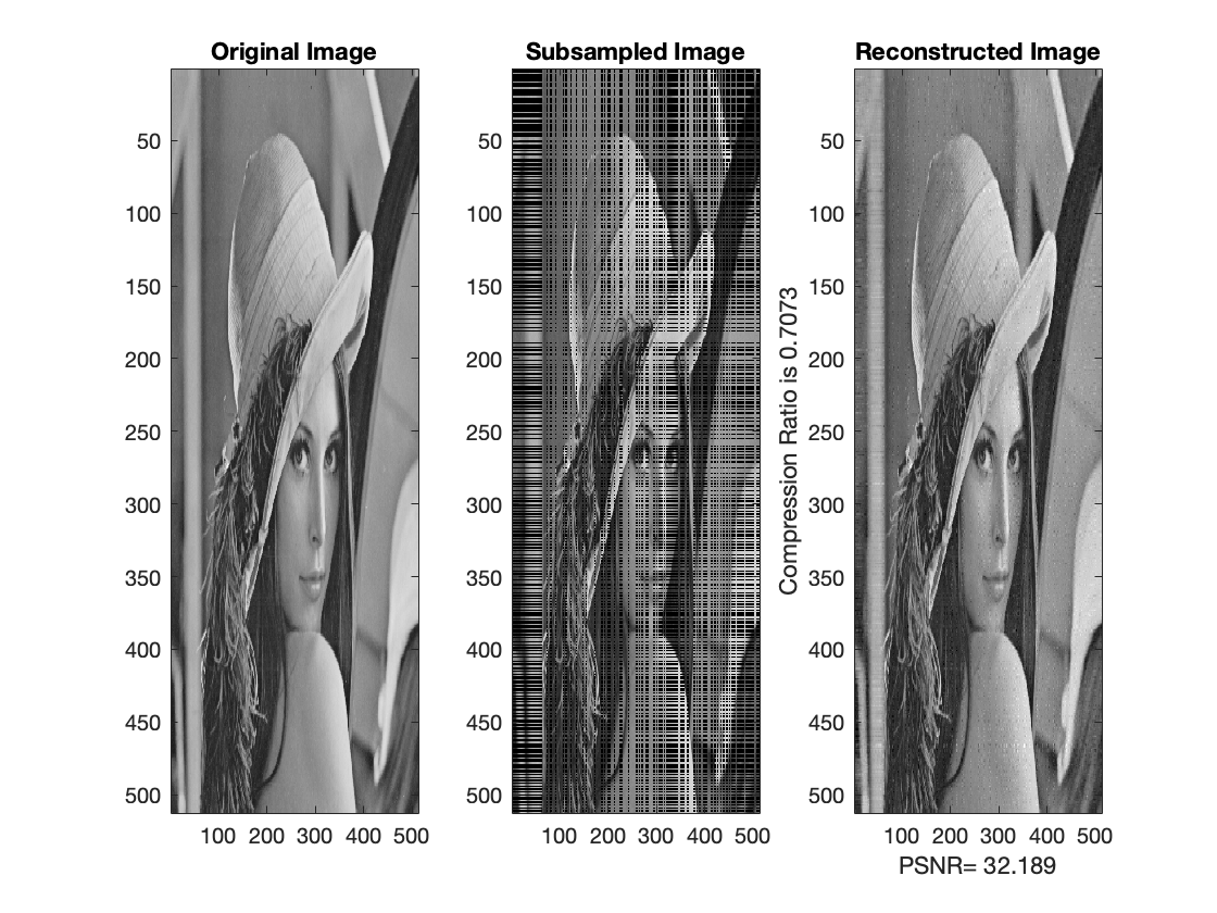
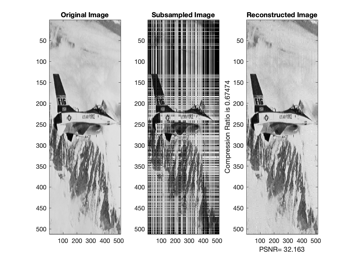
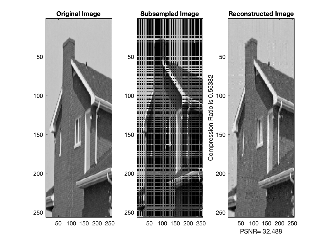
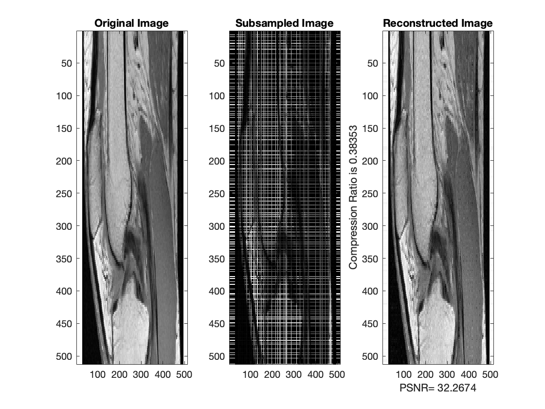
In the following, We use 13 standard images to test our method and report our results in Table 5. That is, the PSNR for these images with their ranks are shown in Table 5. In addition, in Figure 1, we show the comparison of the original images with reconstructed images from their matrix cross approximation. Table 5 shows that many images can be recovered to have PSNR 32 or better by using fewer than half of the integer entries of the entire matrix. In other words, about the half of the pixel values are needed to be encoded for compression instead of the entire image.

Table 5: Various image compression results
image names m n rank Ratio PSNR
bank.pgm 512 512 355 0.90 32.12
barbara.pgm 512 512 260 0.76 32.22
clock.pgm 256 256 90 0.58 32.48
lena512.pgm 512 512 240 0.72 32.20
house.pgm 256 256 90 0.58 32.38
myboat.pgm 256 256 135 0.78 32.80
saturn.pgm 512 512 55 0.20 32.21
F16.pgm 512 512 235 0.71 32.21
pepper.pgm 512 512 370 0.92 32.23
knee.pgm 512 512 105 0.37 32.24
brain.pgm 512 512 110 0.38 32.62
mri.pgm 512 512 130 0.44 34.46
Refer to caption Refer to caption
Figure 1: Comparison of Original Images, Subsampled Images, and Reconstructed Images from Our Method

5.3 Application to Least Squares Approximation

We now turn our attention to the approximation of least squares problem min𝐱A𝐱𝐛subscript𝐱norm𝐴𝐱𝐛\min_{\bf x}\|A{\bf x}-{\bf b}\| for a given observation matrix A𝐴A and observation vector 𝐛𝐛{\bf b}. We shall write 𝐱𝐛subscript𝐱𝐛{\bf x}_{{\bf b}} to the least square solution and explain how to use the matrix cross approximation to find a good approximation of 𝐱𝐛subscript𝐱𝐛{\bf x}_{{\bf b}}. As explained before, we shall use A:,JAI,J1AI,:subscript𝐴:𝐽superscriptsubscript𝐴𝐼𝐽1subscript𝐴𝐼:A_{:,J}A_{I,J}^{-1}A_{I,:} to approximate the observation matrix A𝐴A. For convenience, let us write

A=[AI,JAI,JcAIc,JAIc,Jc].𝐴matrixsubscript𝐴𝐼𝐽subscript𝐴𝐼superscript𝐽𝑐subscript𝐴superscript𝐼𝑐𝐽subscript𝐴superscript𝐼𝑐superscript𝐽𝑐A=\begin{bmatrix}A_{I,J}&A_{I,J^{c}}\\ A_{I^{c},J}&A_{I^{c},J^{c}}\end{bmatrix}. (28)

The matrix cross approximation is

A:,JAI,J1AI,:=[AI,JAIc,J]AI,J1[AI,JAI,Jc]=[EIAIc,JAI,J1][AI,JAI,Jc],subscript𝐴:𝐽superscriptsubscript𝐴𝐼𝐽1subscript𝐴𝐼:matrixsubscript𝐴𝐼𝐽subscript𝐴superscript𝐼𝑐𝐽superscriptsubscript𝐴𝐼𝐽1matrixsubscript𝐴𝐼𝐽subscript𝐴𝐼superscript𝐽𝑐matrixsubscript𝐸𝐼subscript𝐴superscript𝐼𝑐𝐽superscriptsubscript𝐴𝐼𝐽1matrixsubscript𝐴𝐼𝐽subscript𝐴𝐼superscript𝐽𝑐A_{:,J}A_{I,J}^{-1}A_{I,:}=\begin{bmatrix}A_{I,J}\\ A_{I^{c},J}\end{bmatrix}A_{I,J}^{-1}\begin{bmatrix}A_{I,J}&A_{I,J^{c}}\end{bmatrix}=\begin{bmatrix}E_{I}\\ A_{I^{c},J}A_{I,J}^{-1}\end{bmatrix}\begin{bmatrix}A_{I,J}&A_{I,J^{c}}\end{bmatrix}, (29)

where EIsubscript𝐸𝐼E_{I} is the identity matrix. For simplicity, we use Theorem 3 to have

AIc,JcAIc,JAI,J1AI,JcCr+11+rσr+12(A)(r+1)A22σr+1(A).subscriptnormsubscript𝐴superscript𝐼𝑐superscript𝐽𝑐subscript𝐴superscript𝐼𝑐𝐽superscriptsubscript𝐴𝐼𝐽1subscript𝐴𝐼superscript𝐽𝑐𝐶𝑟11𝑟subscriptsuperscript𝜎2𝑟1𝐴𝑟1subscriptsuperscriptnorm𝐴22subscript𝜎𝑟1𝐴\|A_{I^{c},J^{c}}-A_{I^{c},J}A_{I,J}^{-1}A_{I,J^{c}}\|_{C}\leq\frac{r+1}{\sqrt{1+\frac{r\sigma^{2}_{r+1}(A)}{(r+1)\|A\|^{2}_{2}}}}\sigma_{r+1}(A). (30)

Note that all the entries in AIc,JAI,J1subscript𝐴superscript𝐼𝑐𝐽superscriptsubscript𝐴𝐼𝐽1A_{I^{c},J}A_{I,J}^{-1} are less than or equal to 1 in absolute value. One way to find an approximation of the least squares solution is to solve

[AI,JAI,Jc]𝐱^=𝐛Imatrixsubscript𝐴𝐼𝐽subscript𝐴𝐼superscript𝐽𝑐^𝐱subscript𝐛𝐼\begin{bmatrix}A_{I,J}&A_{I,J^{c}}\end{bmatrix}\mathbf{\hat{x}}=\mathbf{b}_{I} (31)

where 𝐛=[𝐛I;𝐛Ic]𝐛subscript𝐛𝐼subscript𝐛superscript𝐼𝑐\mathbf{b}=[\mathbf{b}_{I};\mathbf{b}_{I^{c}}] consists of two parts according to the indices in I𝐼I and the complement indices in Icsuperscript𝐼𝑐I^{c}. Such a solution can be solved using the sparse solution techniques as discussed in [24] or simply solve AI,J𝐱^=𝐛Isubscript𝐴𝐼𝐽^𝐱subscript𝐛𝐼A_{I,J}\mathbf{\hat{x}}=\mathbf{b}_{I} with zero entries in 𝐱𝐱{\bf x} associated with the indices in Jcsuperscript𝐽𝑐J^{c}. Hence, there is no residual or near zero residual in the first part. Our main concern is the residual vector in the second part

[AIc,JAIc,Jc]𝐱^𝐛Ic=AIc,J𝐱^𝐛Ic=AIc,JAI,J1𝐛I𝐛Ic.matrixsubscript𝐴superscript𝐼𝑐𝐽subscript𝐴superscript𝐼𝑐superscript𝐽𝑐^𝐱subscript𝐛superscript𝐼𝑐subscript𝐴superscript𝐼𝑐𝐽^𝐱subscript𝐛superscript𝐼𝑐subscript𝐴superscript𝐼𝑐𝐽superscriptsubscript𝐴𝐼𝐽1subscript𝐛𝐼subscript𝐛superscript𝐼𝑐\begin{bmatrix}A_{I^{c},J}&A_{I^{c},J^{c}}\end{bmatrix}\mathbf{\hat{x}}-\mathbf{b}_{I^{c}}=A_{I^{c},J}\mathbf{\hat{x}}-\mathbf{b}_{I^{c}}=A_{I^{c},J}A_{I,J}^{-1}\mathbf{b}_{I}-\mathbf{b}_{I^{c}}. (32)

Recall 𝐱𝐛subscript𝐱𝐛{\bf x}_{\bf b} is a least squares solution. Wet us write the residual vector A𝐱𝐛𝐛=:ϵA\mathbf{x}_{\bf b}-\mathbf{b}=:\mathbf{\epsilon} with ϵitalic-ϵ\mathbf{\epsilon} consisting of two parts, i.e., ϵ=[ϵI;ϵIc]italic-ϵsubscriptitalic-ϵ𝐼subscriptitalic-ϵsuperscript𝐼𝑐\mathbf{\epsilon}=[\mathbf{\epsilon}_{I};\mathbf{\epsilon}_{I^{c}}]. Then 𝐛Ic=[AIc,JAIc,Jc]𝐱bϵIcsubscript𝐛superscript𝐼𝑐matrixsubscript𝐴superscript𝐼𝑐𝐽subscript𝐴superscript𝐼𝑐superscript𝐽𝑐subscript𝐱𝑏subscriptitalic-ϵsuperscript𝐼𝑐\mathbf{b}_{I^{c}}=\begin{bmatrix}A_{I^{c},J}&A_{I^{c},J^{c}}\end{bmatrix}\mathbf{x}_{b}-\epsilon_{I^{c}}. We have

AIc,J𝐱^𝐛Icsubscript𝐴superscript𝐼𝑐𝐽^𝐱subscript𝐛superscript𝐼𝑐\displaystyle A_{I^{c},J}\mathbf{\hat{x}}-\mathbf{b}_{I^{c}} =AIc,JAI,J1𝐛I𝐛Icabsentsubscript𝐴superscript𝐼𝑐𝐽superscriptsubscript𝐴𝐼𝐽1subscript𝐛𝐼subscript𝐛superscript𝐼𝑐\displaystyle=A_{I^{c},J}A_{I,J}^{-1}\mathbf{b}_{I}-\mathbf{b}_{I^{c}}
=AIc,JAI,J1𝐛I[AIc,JAIc,Jc]𝐱b+ϵIcabsentsubscript𝐴superscript𝐼𝑐𝐽superscriptsubscript𝐴𝐼𝐽1subscript𝐛𝐼matrixsubscript𝐴superscript𝐼𝑐𝐽subscript𝐴superscript𝐼𝑐superscript𝐽𝑐subscript𝐱𝑏subscriptitalic-ϵsuperscript𝐼𝑐\displaystyle=A_{I^{c},J}A_{I,J}^{-1}\mathbf{b}_{I}-\begin{bmatrix}A_{I^{c},J}&A_{I^{c},J^{c}}\end{bmatrix}\mathbf{x}_{b}+\epsilon_{I^{c}}
=AIc,JAI,J1𝐛I[AIc,JAIc,JAI,J1AI,Jc]𝐱b+[0Ic,JAIc,JAI,J1AI,JcAIc,Jc]𝐱b+ϵIcabsentsubscript𝐴superscript𝐼𝑐𝐽superscriptsubscript𝐴𝐼𝐽1subscript𝐛𝐼matrixsubscript𝐴superscript𝐼𝑐𝐽subscript𝐴superscript𝐼𝑐𝐽subscriptsuperscript𝐴1𝐼𝐽subscript𝐴𝐼superscript𝐽𝑐subscript𝐱𝑏matrixsubscript0superscript𝐼𝑐𝐽subscript𝐴superscript𝐼𝑐𝐽subscriptsuperscript𝐴1𝐼𝐽subscript𝐴𝐼superscript𝐽𝑐subscript𝐴superscript𝐼𝑐superscript𝐽𝑐subscript𝐱𝑏subscriptitalic-ϵsuperscript𝐼𝑐\displaystyle=A_{I^{c},J}A_{I,J}^{-1}\mathbf{b}_{I}-\begin{bmatrix}A_{I^{c},J}&A_{I^{c},J}A^{-1}_{I,J}A_{I,J^{c}}\end{bmatrix}\mathbf{x}_{b}+\begin{bmatrix}0_{I^{c},J}&A_{I^{c},J}A^{-1}_{I,J}A_{I,J^{c}}-A_{I^{c},J^{c}}\end{bmatrix}\mathbf{x}_{b}+\epsilon_{I^{c}}
=AIc,JAI,J1(𝐛I[AI,JAI,Jc]𝐱b)+[0Ic,JAIc,JAI,J1AI,JcAIc,Jc]𝐱b+ϵIcabsentsubscript𝐴superscript𝐼𝑐𝐽superscriptsubscript𝐴𝐼𝐽1subscript𝐛𝐼matrixsubscript𝐴𝐼𝐽subscript𝐴𝐼superscript𝐽𝑐subscript𝐱𝑏matrixsubscript0superscript𝐼𝑐𝐽subscript𝐴superscript𝐼𝑐𝐽subscriptsuperscript𝐴1𝐼𝐽subscript𝐴𝐼superscript𝐽𝑐subscript𝐴superscript𝐼𝑐superscript𝐽𝑐subscript𝐱𝑏subscriptitalic-ϵsuperscript𝐼𝑐\displaystyle=A_{I^{c},J}A_{I,J}^{-1}(\mathbf{b}_{I}-\begin{bmatrix}A_{I,J}&A_{I,J^{c}}\end{bmatrix}\mathbf{x}_{b})+\begin{bmatrix}0_{I^{c},J}&A_{I^{c},J}A^{-1}_{I,J}A_{I,J^{c}}-A_{I^{c},J^{c}}\end{bmatrix}\mathbf{x}_{b}+\epsilon_{I^{c}}
=AIc,JAI,J1ϵI+[0Ic,JAIc,JAI,J1AI,JcAIc,Jc]𝐱b+ϵIc.absentsubscript𝐴superscript𝐼𝑐𝐽superscriptsubscript𝐴𝐼𝐽1subscriptitalic-ϵ𝐼matrixsubscript0superscript𝐼𝑐𝐽subscript𝐴superscript𝐼𝑐𝐽subscriptsuperscript𝐴1𝐼𝐽subscript𝐴𝐼superscript𝐽𝑐subscript𝐴superscript𝐼𝑐superscript𝐽𝑐subscript𝐱𝑏subscriptitalic-ϵsuperscript𝐼𝑐\displaystyle=A_{I^{c},J}A_{I,J}^{-1}\epsilon_{I}+\begin{bmatrix}0_{I^{c},J}&A_{I^{c},J}A^{-1}_{I,J}A_{I,J^{c}}-A_{I^{c},J^{c}}\end{bmatrix}\mathbf{x}_{b}+\epsilon_{I^{c}}.

It follows that

A𝐱^𝐛subscriptnorm𝐴^𝐱𝐛\displaystyle\|A\mathbf{\hat{x}}-\mathbf{b}\|_{\infty} =AIc,J𝐱^𝐛Icabsentsubscriptnormsubscript𝐴superscript𝐼𝑐𝐽^𝐱subscript𝐛superscript𝐼𝑐\displaystyle=\|A_{I^{c},J}\mathbf{\hat{x}}-\mathbf{b}_{I^{c}}\|_{\infty} (33)
AIc,JAI,J1ϵI+AIc,JAI,J1AI,JcAIc,JcC𝐱b1+ϵIcabsentsubscriptnormsubscript𝐴superscript𝐼𝑐𝐽subscriptsuperscript𝐴1𝐼𝐽subscriptitalic-ϵ𝐼subscriptnormsubscript𝐴superscript𝐼𝑐𝐽subscriptsuperscript𝐴1𝐼𝐽subscript𝐴𝐼superscript𝐽𝑐subscript𝐴superscript𝐼𝑐superscript𝐽𝑐𝐶subscriptnormsubscript𝐱𝑏1subscriptnormsubscriptitalic-ϵsuperscript𝐼𝑐\displaystyle\leq\|A_{I^{c},J}A^{-1}_{I,J}\epsilon_{I}\|_{\infty}+\|A_{I^{c},J}A^{-1}_{I,J}A_{I,J^{c}}-A_{I^{c},J^{c}}\|_{C}\|\mathbf{x}_{b}\|_{1}+\|\epsilon_{I^{c}}\|_{\infty}
ϵI1+AIc,JAI,J1AI,JcAIc,JcC𝐱b1+ϵIc.absentsubscriptnormsubscriptitalic-ϵ𝐼1subscriptnormsubscript𝐴superscript𝐼𝑐𝐽subscriptsuperscript𝐴1𝐼𝐽subscript𝐴𝐼superscript𝐽𝑐subscript𝐴superscript𝐼𝑐superscript𝐽𝑐𝐶subscriptnormsubscript𝐱𝑏1subscriptnormsubscriptitalic-ϵsuperscript𝐼𝑐\displaystyle\leq\|\epsilon_{I}\|_{1}+\|A_{I^{c},J}A^{-1}_{I,J}A_{I,J^{c}}-A_{I^{c},J^{c}}\|_{C}\|\mathbf{x}_{b}\|_{1}+\|\epsilon_{I^{c}}\|_{\infty}.

since all the entries of AIc,JAI,J1subscript𝐴superscript𝐼𝑐𝐽superscriptsubscript𝐴𝐼𝐽1A_{I^{c},J}A_{I,J}^{-1} are less than or equal to 1 in absolute value, By applying (30), we have established the following main result in this section:

Theorem 8

Let ϵ=[ϵI;ϵIc]italic-ϵsubscriptitalic-ϵ𝐼subscriptitalic-ϵsuperscript𝐼𝑐\mathbf{\epsilon}=[\mathbf{\epsilon}_{I};\mathbf{\epsilon}_{I^{c}}] and let the residual vector A𝐱𝐛𝐛=ϵ𝐴subscript𝐱𝐛𝐛italic-ϵA\mathbf{x}_{\bf b}-\mathbf{b}=\mathbf{\epsilon}. Then

A𝐱^𝐛ϵI1+r+11+rσr+12(A)(r+1)A22σr+1(A)𝐱b1+ϵIc.subscriptnorm𝐴^𝐱𝐛subscriptnormsubscriptitalic-ϵ𝐼1𝑟11𝑟subscriptsuperscript𝜎2𝑟1𝐴𝑟1subscriptsuperscriptnorm𝐴22subscript𝜎𝑟1𝐴subscriptnormsubscript𝐱𝑏1subscriptnormsubscriptitalic-ϵsuperscript𝐼𝑐\|A\mathbf{\hat{x}}-\mathbf{b}\|_{\infty}\leq\|\mathbf{\epsilon}_{I}\|_{1}+\frac{r+1}{\sqrt{1+\frac{r\sigma^{2}_{r+1}(A)}{(r+1)\|A\|^{2}_{2}}}}\sigma_{r+1}(A)\|\mathbf{x}_{b}\|_{1}+\|\mathbf{\epsilon}_{I^{c}}\|_{\infty}. (34)

The solution 𝐱^^𝐱\mathbf{\hat{x}} to (31) is much faster and the residual has a similar estimate as the original least squares solution if σr+1(A)1much-less-thansubscript𝜎𝑟1𝐴1\sigma_{r+1}(A)\ll 1. The computational time is spent on finding a dominant matrix which is dependent on the number of iterations (MATLAB backslash) of matrices of size r×r𝑟𝑟r\times r in Greedy Maximal Volume Algorithms discussed in the previous section. This new computational method will be useful when dealing with least squares tasks which have multiple right-hand side vectors.

Traditionally, we often use the well-known singular value decomposition (SVD) to solve the least squares problem. The computational method explained above has an distinct feature that the SVD does not have. Let us use the following numerical example to illustrate the feature.

Now let us present some numerical examples of finding the best least squares approximation of functions of two variables by using a polynomial basis. In general, this scheme can be applied to any dimensional function approximation. Suppose that we use polynomials of degrees less or equal to 10, i.e. basis functions 1,x,y,x2,xy,y2,,y101𝑥𝑦superscript𝑥2𝑥𝑦superscript𝑦2superscript𝑦101,x,y,x^{2},xy,y^{2},\cdots,y^{10} to find the best coefficients c0,c1,,c65subscript𝑐0subscript𝑐1subscript𝑐65c_{0},c_{1},\cdots,c_{65} such that

minc0,,c65f(x,y)(c0+c1x+c2y++c65y10)L2subscriptsubscript𝑐0subscript𝑐65subscriptnorm𝑓𝑥𝑦subscript𝑐0subscript𝑐1𝑥subscript𝑐2𝑦subscript𝑐65superscript𝑦10superscript𝐿2\min_{c_{0},\cdots,c_{65}}\|f(x,y)-(c_{0}+c_{1}x+c_{2}y+\cdots+c_{65}y^{10})\|_{L^{2}} (35)

for (x,y)[1,1]2𝑥𝑦superscript112(x,y)\in[-1,1]^{2}. We can approximate (35) by using discrete least squares method, i.e., we find the coefficients 𝐜=(c0,,cn)𝐜subscript𝑐0subscript𝑐𝑛\mathbf{c}=(c_{0},\cdots,c_{n}) such that

minc0,,cnf(𝐱j)i=0nciϕi(𝐱j)2,subscriptsubscript𝑐0subscript𝑐𝑛subscriptnorm𝑓subscript𝐱𝑗superscriptsubscript𝑖0𝑛subscript𝑐𝑖subscriptitalic-ϕ𝑖subscript𝐱𝑗superscript2\min_{c_{0},\cdots,c_{n}}\|f(\mathbf{x}_{j})-\sum_{i=0}^{n}c_{i}\phi_{i}(\mathbf{x}_{j})\|_{\ell^{2}}, (36)

where ϕisubscriptitalic-ϕ𝑖\phi_{i}’s are the polynomial basis functions and 𝐱jsubscript𝐱𝑗\mathbf{x}_{j}’s are the sampled points in [1,1]2superscript112[-1,1]^{2} with n1much-greater-than𝑛1n\gg 1.

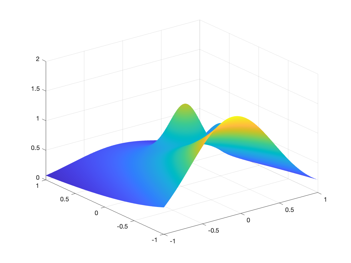
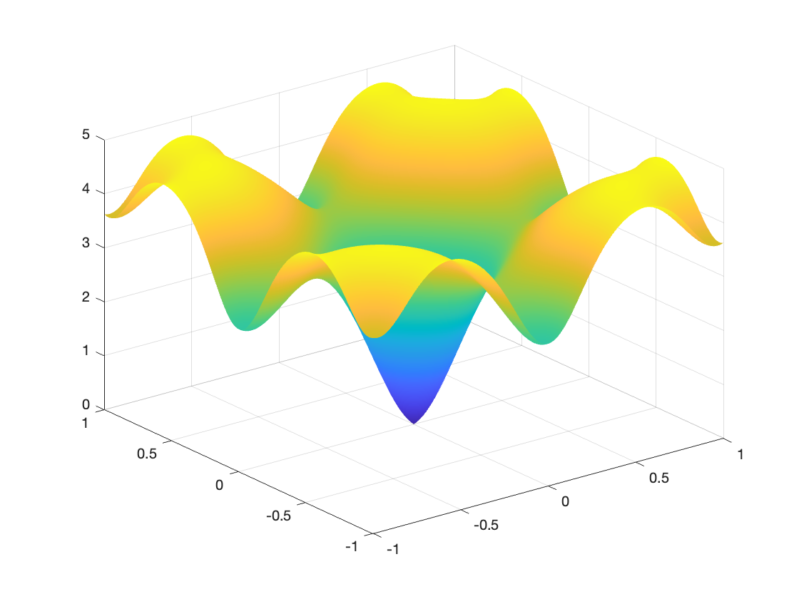
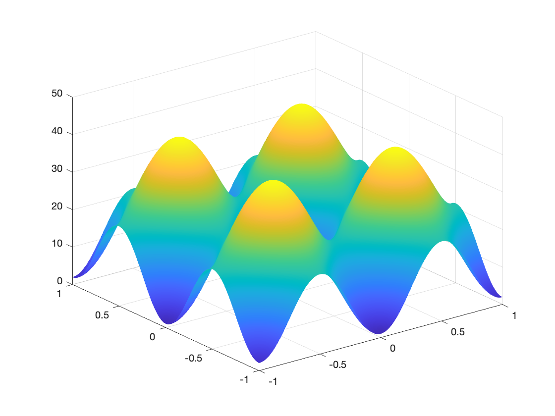
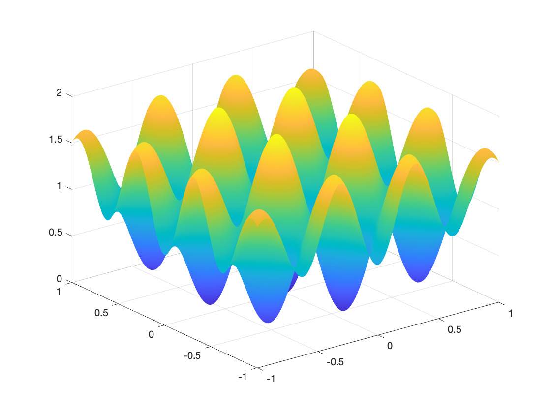
In our experiments, we select continuous functions across different families such as ex2+y2superscript𝑒superscript𝑥2superscript𝑦2e^{x^{2}+y^{2}}, sin(x2+y2)superscript𝑥2superscript𝑦2\sin(x^{2}+y^{2}), cos(x2+y2)superscript𝑥2superscript𝑦2\cos(x^{2}+y^{2}), ln(1+x2+y2)1superscript𝑥2superscript𝑦2\ln(1+x^{2}+y^{2}), (1+x4+y4)/(1+x2+y2)1superscript𝑥4superscript𝑦41superscript𝑥2superscript𝑦2(1+x^{4}+y^{4})/(1+x^{2}+y^{2}), Franke’s function, Ackley’s function, Rastrigin’s function, and wavy function as the testing functions to demonstrate the performances. Some plots of the functions are shown in Figure 3.

We uniformly sampled 512superscript51251^{2} points over [1,1]2superscript112[-1,1]^{2} to solve for an estimated 𝐜^^𝐜\hat{\mathbf{c}} of 𝐜𝐜\mathbf{c} of the discrete least squares problem (36). We report the relative error between the estimated f^^𝑓\hat{f} with the coefficient vector 𝐜^^𝐜\hat{\mathbf{c}} and the exact function f𝑓f in Table 6. The relative errors are computed based on 5012superscript5012501^{2} points over [1,1]2superscript112[-1,1]^{2}.

Refer to caption
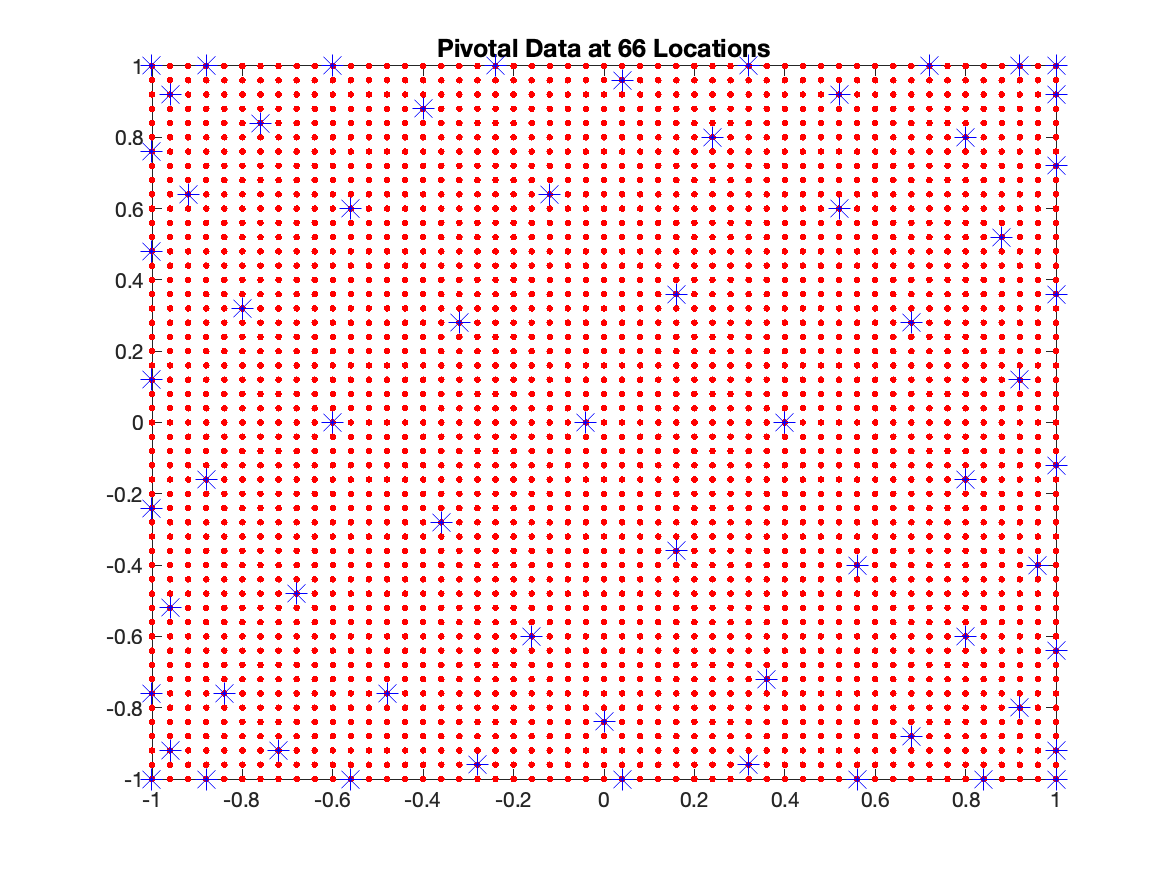
Figure 2: The entire data locations (red) and the pivotal data locations (blue).

Alternatively, we use our matrix cross approximation technique to select some rows and columns as discussed before and then solve a smaller discrete least squares problem. It is worthy noting that our data matrix [ϕi(𝐱j)]i,jsubscriptdelimited-[]subscriptitalic-ϕ𝑖subscript𝐱𝑗𝑖𝑗[\phi_{i}(\mathbf{x}_{j})]_{i,j} in this setup is of full column rank, therefore the second term in the right side of (34) is zero and our GMVA is going to select all the rows together with the same number of columns. Let us call these selected rows the pivotal rows, or pivotal sample locations, we can solve (36) only based on those 𝐱jsubscript𝐱𝑗\mathbf{x}_{j}’s which belong to the pivotal sample locations to get an estimated f^psubscript^𝑓𝑝\hat{f}_{p} of f𝑓f. Figure 2 shows the pivotal locations of the uniform sampling. We also report the relative error between f^psubscript^𝑓𝑝\hat{f}_{p} and the exact testing function f𝑓f in Table 6. Again the relative errors are computed based on 5012superscript5012501^{2} points over [1,1]2superscript112[-1,1]^{2}.

We can see that the two columns of relative errors in Table 6 are in the same magnitude, which shows that we just need to use the data at pivotal locations to have a good approximation instead of the entire data 512superscript51251^{2} locations. That is, our computational method for the least squares solution reveals the pivotal locations in [1,1]2superscript112[-1,1]^{2} for measuring the unknown target functions so that we can use fewer measurements and quickly recover them.

Table 6: Relative errors of least squares approximations for functions of two variables by using 512superscript51251^{2} sample locations and by using pivotal data locations
f(x,y)𝑓𝑥𝑦f(x,y) ff^relsubscriptnorm𝑓^𝑓𝑟𝑒𝑙\|f-\hat{f}\|_{rel} ff^prelsubscriptnorm𝑓subscript^𝑓𝑝𝑟𝑒𝑙\|f-\hat{f}_{p}\|_{rel}
ex2+y2superscript𝑒superscript𝑥2superscript𝑦2e^{x^{2}+y^{2}} 1.93E-05 4.59E-05
sin(x2+y2)superscript𝑥2superscript𝑦2\sin(x^{2}+y^{2}) 2.13E-05 5.07E-05
cos(x2+y2)superscript𝑥2superscript𝑦2\cos(x^{2}+y^{2}) 1.28E-05 2.83E-05
ln(1+x2+y2)1superscript𝑥2superscript𝑦2\ln(1+x^{2}+y^{2}) 1.06E-04 2.10E-04
(1+x4+y4)/(1+x2+y2)1superscript𝑥4superscript𝑦41superscript𝑥2superscript𝑦2(1+x^{4}+y^{4})/(1+x^{2}+y^{2}) 3.40E-04 6.57E-04
Franke’s function 5.90E-02 8.10E-02
Ackley’s function 2.10E-02 4.05E-02
Rastrigin’s function 7.65E-04 1.10E-03
Wavy function 7.03E-02 9.80E-02
Refer to caption Refer to caption
Figure 3: Plot of some testing functions (top row: Franke and Ackley. bottom row: Rastrigin and wavy).

6 Conclusion and Future Research

In this work, we proposed a family of greedy based maximal volume algorithms which improve the classic maximal volume algorithm in terms of the error bound of matrix cross approximation and the computational efficiency. The proposed algorithms are shown to have theoretical guarantees on convergence and are demonstrated to have nice performances on the applications such as image compression and least squares solution.

Future research can be conducted along the following directions. Firstly, although the improved error bound in Theorem 3 is slightly better than its previous counterpart, we would like to seek for an error bound which is even tighter and an algorithm which can achieve this tighter error bound. Secondly, as data matrices in the real-world applications are usually incomplete or not fully observable, it is vital to generalize the algorithms to the setting which can fit in the case where matrices have missing values. Thirdly, if a matrix is sparse or special structured, we want to develop some more pertinent algorithm to have a better approximation result. Finally, we plan to generalize the proposed approach to the setting of tensor production approximation of high dimensional functions.

Acknowledgements

The second author would like to acknowledge the Simon Foundation for collaboration grant #864439.

References

  • [1] K. Allen, A Geometric Approach to Low-Rank Matrix and Tensor Completion, Dissertation, University of Georgia, 2021.
  • [2] J. Bennett, C. Elkan, B. Liu, P. Smyth, D. Tikk. Kdd cup and workshop 2007. ACM SIGKDD explorations newsletter 9, no. 2 (2007): 51-52.
  • [3] A. Ben-Israel, A volume associated with m×n𝑚𝑛m\times n matrices, Linear Algebra Appl., 167, 1992.
  • [4] C. Boutsidis and D. P. Woodruff. Optimal CUR matrix decompositions. In Proceedings of the forty-sixth annual ACM symposium on Theory of computing, pp. 353-362. 2014.
  • [5] H. Cai, K. Hamm, L. Huang, J. Li, and T. Wang. ”Rapid robust principal component analysis: CUR accelerated inexact low rank estimation.” IEEE Signal Processing Letters 28 (2020): 116-120.
  • [6] H, Cai, K. Hamm, L. Huang, D. Needell. Mode-wise tensor decompositions: Multi-dimensional generalizations of CUR decompositions. The Journal of Machine Learning Research 22, no. 1 (2021): 8321-8356.
  • [7] H. Cai, L. Huang, P. Li, D. Needell. Matrix completion with cross-concentrated sampling: Bridging uniform sampling and CUR sampling. IEEE Transactions on Pattern Analysis and Machine Intelligence (2023).
  • [8] J.-F. Cai, T. Wang, K. Wei. Fast and provable algorithms for spectrally sparse signal reconstruction via low-rank Hankel matrix completion. Applied and Computational Harmonic Analysis 46, no. 1 (2019): 94-121.
  • [9] E. Candes and J. Romberg. Sparsity and incoherence in compressive sampling. Inverse problems 23, no. 3 (2007): 969.
  • [10] E. Candes and B. Recht. Exact matrix completion via convex optimization. Communications of the ACM 55, no. 6 (2012): 111-119.
  • [11] S. Chaturantabut and D. C. Sorensen. Nonlinear model reduction via discrete empirical interpolation. SIAM Journal on Scientific Computing 32, no. 5 (2010): 2737-2764.
  • [12] A. Civril and M. M. Ismail, On selecting a maximum volume submatrix of a matrix and related problems, Theo. Comp. Sci., 410, 4801–4811, 2009.
  • [13] P. Drineas, M. W. Mahoney, S. Muthukrishnan. Relative-error CUR matrix decompositions. SIAM Journal on Matrix Analysis and Applications 30, no. 2 (2008): 844-881.
  • [14] Z. Drmac and S. Gugercin. A new selection operator for the discrete empirical interpolation method—improved a priori error bound and extensions. SIAM Journal on Scientific Computing 38, no. 2 (2016): A631-A648.
  • [15] M. Fazel, E. Candes, B. Recht, P. Parrilo. Compressed sensing and robust recovery of low rank matrices. In 2008 42nd Asilomar Conference on Signals, Systems and Computers, pp. 1043-1047. IEEE, 2008.
  • [16] I. Georgieva and C. Hofreithery, On the Best Uniform Approximation by Low-Rank Matrices, Linear Algebra and its Applications, vol.518(2017), Pages 159–176.
  • [17] D. Goldberg, D. Nichols, B. M. Oki, D. Terry. Using collaborative filtering to weave an information tapestry. Communications of the ACM 35, no. 12 (1992): 61-70.
  • [18] S. A. Goreinov, E. E. Tyrtyshnikov, and N. L. Zamarashkin. A theory of pseudoskeleton approximations. Linear algebra and its applications 261, no. 1-3 (1997): 1-21.
  • [19] S. A. Goreinov, I. V. Oseledets, D. V. Savostyanov, E. E. Tyrtyshnikov, N. L. Zamarashkin. How to find a good submatrix. In Matrix Methods: Theory, Algorithms And Applications: Dedicated to the Memory of Gene Golub, pp. 247-256. 2010.
  • [20] S. A. Goreinov and E. E. Tyrtyshnikov, The maximal-volume concept in approximation by low-rank matrices, Contemporary Mathematics, 208: 47–51, 2001.
  • [21] K. Hamm and L. Huang. Perspectives on CUR decompositions. Applied and Computational Harmonic Analysis 48, no. 3 (2020): 1088-1099.
  • [22] K. Hamm, L. Huang, Stability of Sampling for CUR Decomposition, Foundations of Data Science, Vol. 2, No. 2 (2020), 83-99.
  • [23] N. Kishore Kumar and J. Schneider, Literature survey on low rank approximation of matrices, Journal on Linear and Multilinear Algebra, vol. 65 (2017), 2212–2244.
  • [24] M.-J. Lai and Y. Wang. Sparse Solutions of Underdetermined Linear Systems and Their Applications, Society for Industrial and Applied Mathematics, 2021.
  • [25] N. Mitrovic, M. T. Asif, U. Rasheed, J. Dauwels, and P. Jaillet. ”CUR decomposition for compression and compressed sensing of large-scale traffic data.” In 16th International IEEE Conference on Intelligent Transportation Systems (ITSC 2013), pp. 1475-1480. IEEE, 2013.
  • [26] M. W. Mahoney and P. Drineas. CUR matrix decompositions for improved data analysis. Proceedings of the National Academy of Sciences 106, no. 3 (2009): 697-702.
  • [27] M. W. Mahoney, M. Maggioni, and Petros Drineas. ”Tensor-CUR decompositions for tensor-based data.” In Proceedings of the 12th ACM SIGKDD international conference on Knowledge discovery and data mining, pp. 327-336. 2006.
  • [28] A. Mikhaleva and I. V. Oseledets, Rectangular maximum-volume submatrices and their applications, Linear Algebra and its Applications, Vol. 538, 2018, Pages 187–211.
  • [29] Ivan Oseledets and Eugene Tyrtyshnikov, TT-cross approximation for multidimensional arrays, Linear Algebra and its Applications, 432 (2010) 70–88.
  • [30] C.-T. Pan. On the existence and computation of rank-revealing LU factorizations. Linear Algebra Appl., 316, 2000.
  • [31] L. Schork and J. Gondzio, Rank revealing Gaussian elimination by the maximum volume concept. Linear Algebra and its Applications, 2020
  • [32] D. C. Sorensen and M. Embree. A DEIM Induced CUR Factorization. SIAM Journal on Scientific Computing 38, no. 3 (2016): A1454-A1482.
  • [33] Z. Wang, M.-J. Lai, Z. Lu, W. Fan, H. Davulcu, and J. Ye. Orthogonal rank-one matrix pursuit for low rank matrix completion. SIAM Journal on Scientific Computing 37, no. 1 (2015): A488-A514.