Directly Fine-Tuning Diffusion Models on Differentiable Rewards

Abstract

We present Direct Reward Fine-Tuning (DRaFT), a simple and effective method for fine-tuning diffusion models to maximize differentiable reward functions, such as scores from human preference models. We first show that it is possible to backpropagate the reward function gradient through the full sampling procedure, and that doing so achieves strong performance on a variety of rewards, outperforming reinforcement learning-based approaches. We then propose more efficient variants of DRaFT: DRaFT-$K$, which truncates backpropagation to only the last $K$ steps of sampling, and DRaFT-LV, which obtains lower-variance gradient estimates for the case when $K=1$. We show that our methods work well for a variety of reward functions and can be used to substantially improve the aesthetic quality of images generated by Stable Diffusion 1.4. Finally, we draw connections between our approach and prior work, providing a unifying perspective on the design space of gradient-based fine-tuning algorithms.

Figure 1: DRaFT using human preference reward models yields more detailed and stylized images than baseline Stable Diffusion. See Figure 35 in Appendix E for more samples.

1 Introduction

Diffusion models (Sohl-Dickstein et al., 2015; Song & Ermon, 2019; Ho et al., 2020; Song et al., 2021b; Kingma et al., 2021) have revolutionized generative modeling for continuous data, achieving impressive results across modalities including images, videos, and audio. However, for many use cases, modeling the training data distribution exactly (e.g. diverse images from the web) does not align with the model’s desired behavior (e.g. generating aesthetically pleasing images). To overcome this mismatch, text-to-image diffusion models commonly employ methods like classifier-free guidance (Ho & Salimans, 2021) to improve image-text alignment, and are fine-tuned on curated datasets such as LAION Aesthetics (Schuhmann & Beaumont, 2022) to improve image quality.

Within the language modeling community, aligning model behavior with human preferences is widely accomplished through fine-tuning with reinforcement learning (RL), such as with RL from human feedback (RLHF; Ziegler et al. 2019; Stiennon et al. 2020; Ouyang et al. 2022; Bai et al. 2022a). Inspired by RLHF, supervised and reinforcement learning methods have been developed to train diffusion models on human preference models or other rewards (Lee et al., 2023; Wu et al., 2023b; Dong et al., 2023; Black et al., 2023; Fan et al., 2023). While showing some success at improving text alignment or image aesthetics on narrow domains, these approaches are sample inefficient and have not been scaled up to the level of generally improving generation style across diverse prompts.

We propose a simple and efficient approach for gradient-based reward fine-tuning, based on differentiating through the diffusion sampling process. We first introduce Direct Reward Fine-Tuning (DRaFT), a conceptually straightforward method that backpropagates through the full sampling chain (e.g., an unrolled computation graph of length 50). To keep memory and compute costs low, we use gradient checkpointing (Chen et al., 2016) and optimize LoRA weights (Hu et al., 2022) rather than the full set of model parameters. Then, we introduce modifications to DRaFT that further improve its efficiency and performance. First, we propose DRaFT-$K$, a variant that backpropagates through only the last $K$ steps of sampling to compute the gradient for fine-tuning. We show empirically that full backpropagation can result in exploding gradients, and that using the truncated gradient performs substantially better given the same number of training steps. Then, we further improve efficiency by introducing DRaFT-LV, a variant of DRaFT-1 that computes lower-variance gradient estimates by averaging over multiple noise samples.

We apply DRaFT to Stable Diffusion 1.4 (Rombach et al., 2022) and evaluate it on a variety of reward functions and prompt sets. As our methods leverage gradients, they are substantially more efficient than RL-based fine-tuning baselines, for example maximizing scores from the LAION Aesthetics Classifier (Schuhmann & Beaumont, 2022) $>\!200\times$ faster than the RL algorithms from Black et al. (2023). DRaFT-LV is particularly efficient, learning roughly 2x faster than ReFL (Xu et al., 2023), a previous gradient-based fine-tuning method. We scale up DRaFT to training on hundreds of thousands of prompts and show that it improves Stable Diffusion on human preference rewards such as PickScore (Kirstain et al., 2023) and Human Preference Score v2 (Wu et al., 2023a). We further show that DRaFT models can be combined or interpolated towards the pre-trained model simply by mixing or scaling the LoRA weights. Finally, we showcase how DRaFT can be easily applied to diverse reward functions by using it to train for image compressibility and incompressibility, object detection and removal, and generating adversarial examples.

2 Related Work

We provide an extended discussion of related work in Appendix D.

Learning human preferences.

Human preference learning trains models on judgements of which behaviors people prefer, rather than on human demonstrations directly (Knox & Stone, 2009; Akrour et al., 2011). This training is commonly done by learning a reward model reflecting human preferences and then learning a policy that maximizes the reward (Christiano et al., 2017; Ibarz et al., 2018). We apply DRaFT to optimize scores from existing preference models, such as PickScore (Kirstain et al., 2023) and Human Preference Score v2 (Wu et al., 2023a), which are trained on human judgements between pairs of images generated by diffusion models for the same prompt.

Guidance (Song et al., 2021b; Dhariwal & Nichol, 2021) steers sampling towards images that satisfy a desired objective by adding an auxiliary term to the score function. Various pre-trained models can be used to provide guidance signals, including classifiers, facial recognition models, and object detectors (Bansal et al., 2023). Noisy examples obtained during sampling may be out-of-distribution for the guidance model. Two approaches to mitigate this are (1) training the guidance model on noisy data (Dhariwal & Nichol, 2021) and (2) applying a guidance model to predicted clean images from one-step denoising (Li et al., 2022). However, (1) precludes the use of off-the-shelf pre-trained guidance functions and (2) applies guidance to out-of-distribution blurry images for high noise levels. DRaFT avoids these issues by only applying the reward function to the final generated image.

Backpropagation through diffusion sampling.

Watson et al. (2021) differentiate through sampling to learn sampler hyperparameters (rather than model parameters) in order to train samplers that reduce inference cost while maintaining perceptual image quality. Like DRaFT, Direct Optimization of Diffusion Latents (DOODL; Wallace et al. 2023) backpropagates through sampling to optimize differentiable rewards; however DOODL optimizes the initial noise sample $\mathbf{x}_{T}$ rather than the model parameters. While this does not require a training phase, it is much slower at inference time because the optimization must be redone for each prompt and metric.

Reward Fine-Tuning with Supervised Learning.

Lee et al. (2023) and Wu et al. (2023b) use supervised approaches to fine-tune diffusion models on rewards. These methods generate images with the pre-trained model and then fine-tune on the images while weighting examples according to the reward function or discarding low-reward examples. Unlike DRaFT or RL methods, the model is not trained online on examples generated by the current policy. However, Dong et al. (2023) use an online version of this approach where examples are re-generated over multiple rounds of training, which can be viewed as a simple kind of reinforcement learning.

Reward Fine-Tuning with Reinforcement Learning.

Black et al. (2023) and Fan et al. (2023) interpret the denoising process as a multi-step decision-making task, and use policy gradient algorithms to fine-tune diffusion models for arbitrary black-box objectives. Rather than optimizing model parameters, Hao et al. (2022) apply RL to improve the input prompts. RL approaches are flexible because they do not require differentiable rewards. However, in practice many reward functions are differentiable, or can be implemented or approximated in a differentiable way, and thus analytic gradients are often available. In such cases, using reinforcement learning discards useful information.

Reward Feedback Learning (ReFL).

ReFL (Xu et al., 2023) uses reward function gradients to fine-tune a diffusion model. It does not backpropagate through sampling, making it similar to DRaFT-1. However, it evaluates the reward on the one-step predicted clean image, $r(\hat{\mathbf{x}}_{0},\mathbf{c})$ from a randomly-chosen step $t$ along the denoising trajectory rather than on the final image. While ReFL performs similarly to DRaFT-1, DRaFT-LV is substantially more efficient, training approximately 2x faster. We further discuss how ReFL relates to DRaFT in Section 4.

3 Background on Diffusion Models

Diffusion Models.

Diffusion models are latent variable models based on the principle of iterative denoising: samples are generated starting from pure noise $\mathbf{x}_{T}\sim\mathcal{N}(\bm{0},\mathbf{I})$ via a sequence of applications of a learned denoising function $\bm{\epsilon}_{{\bm{\theta}}}$ that gradually removes noise over $T$ timesteps. Diffusion models often learn the denoiser $\bm{\epsilon}_{{\bm{\theta}}}$ by minimizing the following re-weighted variational lower bound of the marginal likelihood (Ho et al., 2020):

$$\mathcal{L}_{\text{Simple}}({\bm{\theta}})=\mathbb{E}_{t\sim U(0,T),\mathbf{x}_{0}\sim p_{\text{data}},\bm{\epsilon}\sim\mathcal{N}(\bm{0},\mathbf{I})}\left[\|\bm{\epsilon}-\bm{\epsilon}_{{\bm{\theta}}}\left(\alpha_{t}\mathbf{x}_{0}+\sigma_{t}\bm{\epsilon},t\right)\|^{2}\right]$$ (1)

where $\sigma_{t}=\sqrt{1-\alpha^{2}_{t}}$ is an increasing noise schedule. Here, $\bm{\epsilon}_{{\bm{\theta}}}$ is trained to predict the noise $\bm{\epsilon}$ added to the clean datapoint $\mathbf{x}_{0}$. For image data, $\bm{\epsilon}_{{\bm{\theta}}}$ is typically parameterized by a UNet (Ronneberger et al., 2015). We use conditional diffusion models, which include a context $\mathbf{c}$ such as a text prompt passed to the denoising function $\bm{\epsilon}_{{\bm{\theta}}}(\mathbf{x}_{t},\mathbf{c},t)$. For inference (i.e., sampling), one draws a noise sample $\mathbf{x}_{T}$, and then iteratively uses $\bm{\epsilon}_{\theta}$ to estimate the noise and compute the next latent sample $\mathbf{x}_{t-1}$.

Classifier-Free Guidance.

Classifier-free guidance (CFG) uses a linear combination of the conditional and unconditional score estimates, denoising according to $(1+w(t))\bm{\epsilon}(\mathbf{x}_{t},\mathbf{c},t)-w(t)\bm{\epsilon}(\mathbf{x}_{t},\varnothing,t)$ where $w(t)$ is the guidance weight and $\varnothing$ indicates an empty conditioning signal. It requires that $\mathbf{c}$ is replaced with $\varnothing$ part of the time during training so the unconditional score function is learned.

4 Method

Figure 2: DRaFT backpropagates reward gradients through the sampling process into LoRA weights. DRaFT-$K$ truncates the backward pass, differentiating through only the last $K$ steps of sampling. DRaFT-LV improves the efficiency of DRaFT-1 by generating multiple examples in the last step to reduce variance.

We propose a simple approach for fine-tuning diffusion models for differentiable reward functions. Our goal is to fine-tune the parameters ${\bm{\theta}}$ of a pre-trained diffusion model such that images generated by the sampling process maximize a differentiable reward function $r$:

$$J({\bm{\theta}})=\mathbb{E}_{\mathbf{c}\sim p_{\mathbf{c}},\mathbf{x}_{T}\sim\mathcal{N}(\bm{0},\mathbf{I})}\left[r(\text{sample}({\bm{\theta}},\mathbf{c},\mathbf{x}_{T}),\mathbf{c})\right]$$ (2)

where $\text{sample}({\bm{\theta}},\mathbf{c},\mathbf{x}_{T})$ denotes the sampling process from time $t=T\to 0$ with context $\mathbf{c}$.

DRaFT.

First, we consider solving Eq. 2 by computing $\nabla_{{\bm{\theta}}}r(\text{sample}({\bm{\theta}},\mathbf{c},\mathbf{x}_{T}),\mathbf{c})$ and using gradient ascent. Computing this gradient requires backpropagation through multiple diffusion model calls in the sampling chain, similar to backpropagation through time in a recurrent neural network. We use two approaches to reduce the memory cost of DRaFT: 1) low-rank adaptation (LoRA) (Hu et al., 2022); and 2) gradient checkpointing (Chen et al., 2016).

LoRA.

Rather than fine-tuning the full set of model parameters, Low-Rank Adaptation (LoRA) (Hu et al., 2022) freezes the weights of the pre-trained model, and injects new low-rank weight matrices alongside the original model weights, whose contributions are summed to produce the adapted model outputs. Mathematically, for a layer with base parameters $\mathbf{W}_{0}$ whose forward pass yields $\mathbf{h}=\mathbf{W}_{0}\mathbf{x}$, the LoRA adapted layer is $\mathbf{h}=\mathbf{W}_{0}\mathbf{x}+\mathbf{B}\mathbf{A}\mathbf{x}$, where $\mathbf{B}\mathbf{A}$ is a low-rank matrix. LoRA dramatically reduces the number of parameters that need to be optimized, which reduces the memory requirements of fine-tuning. Another benefit is that, because the information learned by the fine-tuned model is contained within the LoRA parameters, we can conveniently combine fine-tuned models by summing the LoRA parameters (Figure 5, right) and interpolate between the original and fine-tuned model by re-scaling the LoRA parameters (Figure 7).

Algorithm 1 DRaFT (with DDIM sampling)

inputs: pre-trained diffusion model weights ${\bm{\theta}}$, reward $r$, prompt dataset $p_{\mathbf{c}}$

while not converged do

     $t_{\text{truncate}}=\begin{cases}\text{randint}(1,m)&\text{{if} \color[rgb]{0.90625,0.3046875,0}\definecolor[named]{pgfstrokecolor}{rgb}{0.90625,0.3046875,0} ReFL}\\ T&\text{{if} \color[rgb]{0.65234375,0,0.19921875}\definecolor[named]{pgfstrokecolor}{rgb}{0.65234375,0,0.19921875} DRaFT}\\ K&\text{{if} \color[rgb]{0.80078125,0,0.3984375}\definecolor[named]{pgfstrokecolor}{rgb}{0.80078125,0,0.3984375} DRaFT-$K$}\\ 1&\text{{if} \color[rgb]{0,0,0.8125}\definecolor[named]{pgfstrokecolor}{rgb}{0,0,0.8125} DRaFT-LV}\\ \end{cases}$

     $\mathbf{c}\sim p_{\mathbf{c}}$, $\mathbf{x}_{T}\sim\mathcal{N}(\bm{0},\mathbf{I})$

     for $t=T,\dots,1$ do

         if  $t=t_{\text{truncate}}$ then

               $\mathbf{x}_{t}=\texttt{stop\_grad}(\mathbf{x}_{t})$          

         $\hat{\mathbf{x}}_{0}=(\mathbf{x}_{t}-\sigma_{t}\bm{\epsilon}_{{\bm{\theta}}}(\mathbf{x}_{t},\mathbf{c},t))/\alpha_{t}$

         if  $t=t_{\text{truncate}}$ and ReFL then

               $\mathbf{x}_{0}\approx\hat{\mathbf{x}}_{0}$

               break          

         $\mathbf{x}_{t-1}=\alpha_{t-1}\hat{\mathbf{x}}_{0}+\sigma_{t-1}\bm{\epsilon}_{{\bm{\theta}}}(\mathbf{x}_{t},\mathbf{c},t)$      

     $\bm{g}=\nabla_{{\bm{\theta}}}r(\mathbf{x}_{0},\mathbf{c})$

     if  DRaFT-LV then

         for $i=1,\dots,n$ do

              $\bm{\epsilon}\sim\mathcal{N}(\bm{0},\mathbf{I})$

              $\mathbf{x}_{1}=\alpha_{1}\texttt{stop\_grad}(\mathbf{x}_{0})+\sigma_{1}\bm{\epsilon}$

              $\hat{\mathbf{x}}_{0}=(\mathbf{x}_{1}-\sigma_{1}\bm{\epsilon}_{{\bm{\theta}}}(\mathbf{x}_{1},\mathbf{c},1))/\alpha_{1}$

              $\bm{g}=\bm{g}+\nabla_{{\bm{\theta}}}r(\hat{\mathbf{x}}_{0},\mathbf{c})$                

     ${\bm{\theta}}\leftarrow{\bm{\theta}}-\eta\bm{g}$

return ${\bm{\theta}}$

Gradient Checkpointing.

Gradient checkpointing (Gruslys et al., 2016; Chen et al., 2016) reduces the memory cost of storing activations for use during backprop at the cost of increased compute by storing only a subset of activations in memory and re-computing the others on the fly. Specifically, we only store the input latent for each denoising step, and re-materialize the UNet activations during backprop. Implementing checkpointing in JAX (Bradbury et al., 2018) is as simple as adding @jax.checkpoint to the body of the sampling loop.

DRaFT-$K$.

While gradient checkpointing makes it possible to backpropagate through the full sampling chain, we found that optimization speed and overall performance can be substantially improved by truncating backprop through only the last $K$ sampling steps. We call the resulting approach DRaFT-$K$, illustrated in Figure 2. Truncating backprop reduces the compute needed per step by decreasing the number of backward passes through the UNet. Surprisingly, it also improves training efficiency per-step, which we investigate further in Section 5.2.

DRaFT-LV.

Empirically, we find simply setting $K=1$ (i.e., only learning on the last train step) results in the best reward vs. compute tradeoff. Here we propose a method for improving the efficiency of DRaFT-1 further by reducing the variance of the gradient estimate. We call this low-variance estimator DRaFT-LV. The key idea is to use the forward diffusion process to produce additional examples to train on without re-generating new images. Specifically, we noise the generated image $n$ times, and use the summed reward gradient over these examples. Although DRaFT-LV adds $n$ additional forward and backward passes through the UNet and reward model, in practice this is fairly little overhead compared to the $T$ UNet calls already needed for sampling. We found that using $n=2$ is around $2\times$ more efficient than DRaFT-1 while adding around 10% compute overhead for our reward functions.

General Reward Fine-Tuning Algorithm.

Algorithm 1 presents a unified framework encompassing several gradient-based approaches for diffusion fine-tuning. In particular, it includes as special cases DRaFT, DRaFT-$K$, DRaFT-LV, and ReFL (Xu et al., 2023), which differ in how the gradient is computed. DRaFT-$K$ inserts a stop-gradient operation $\mathbf{x}_{t}=\texttt{stop\_grad}(\mathbf{x}_{t})$ at sampling iteration $K$, to ensure that the gradient is only computed through the last $K$ steps; vanilla DRaFT can be obtained by setting $K=T$. ReFL inserts a stop gradient and breaks out of the sampling loop early, returning a one-step predicted clean image. Additionally, it does so at a random timestep towards the end of sampling (we use $m=20$ for 50-step sampling). In this unifying framework, ReFL with $m=1$ is equivalent to DRaFT-$1$. Lastly, DRaFT-LV averages the last-step gradient over multiple examples with different noises to reduce variance. Note that in practice we use Adam and LoRA, which for simplicity are not shown in the algorithm.

5 Experiments

In this section, we show that DRaFT can be applied to a wide range of reward functions, and that it substantially outperforms prior reward fine-tuning methods. We use Stable Diffusion 1.4 as the base diffusion model. As it is a latent diffusion model (Rombach et al., 2022), applying DRaFT means we backpropagate through both the sampling process producing the latent representation and the decoder used to obtain the image. DRaFT is applicable to any differentiable sampler; in our experiments, we used DDIM (Song et al., 2021a), but we found that ancestral sampling performs similarly. We use 50 sampling steps, so DRaFT-50 corresponds to backpropagating through the full sampling chain (i.e., vanilla DRaFT), and a classifier-free guidance weight of 7.5. Experimental details, hyperparameters, and additional results are provided in Appendices A and  B.

5.1 Fine-Tuning for Aesthetic Quality

Figure 3: Left: Sample efficiency of methods when maximizing scores from the LAION Aesthetic Classifier. DDPO (Black et al., 2023) results were obtained from correspondence with the authors, as the results in the original paper use a buggy implementation; DDPO achieves a reward of 7.4 after 50k reward queries. Right: Qualitative comparison of generations as training progresses.

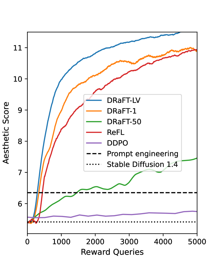
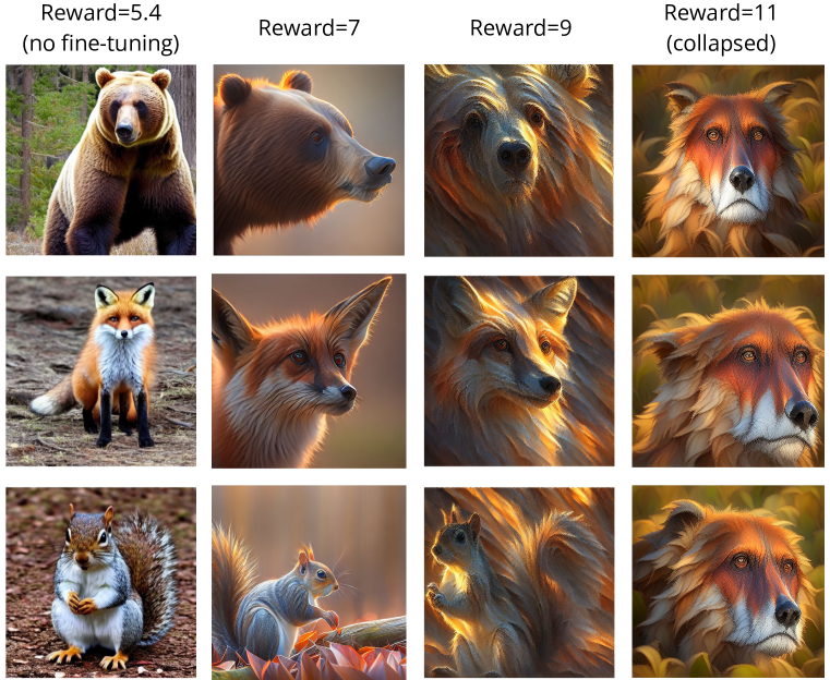
We first compare methods at improving aesthetic quality scores provided by the LAION aesthetic predictor, which is trained to rate images on a scale of 1 through 10. We use the simple set of 45 prompts from Black et al. (2023), where each prompt is the name of a common animal. We compare against the DDPO (Black et al., 2023) RL method, ReFL (Xu et al., 2023), and a prompt engineering baseline (see Appendix A.3 for more details). Results are shown in Figure 3. Because it does not make use of gradients, reinforcement learning is much less sample-efficient that the other methods. Interestingly, truncating DRaFT to a single backwards step substantially improves sample efficiency; we analyze this phenomenon further in Section 5.2. Thanks to its lower-variance gradient estimate, DRaFT-LV further improves training efficiency. We observe that the methods initially produce improved images, but eventually collapse to producing very similar high-reward images.

Reward Hacking.

In Figure 3 (Right), we observe an instance of reward hacking, where the fine-tuned model loses diversity and collapses to generate a certain high-reward image. Reward hacking points to deficiencies in existing rewards, and efficiently finding gaps between the desired behavior and the behavior implicitly captured by the reward is a crucial step in fixing the reward. Improved techniques for fine-tuning, such as DRaFT, can aid the development of new rewards. In Appendix B.8, we include examples of reward hacking that we observed in certain experiments.

5.2 Fine-Tuning on Human Preferences

Figure 4: Comparison of the HPSv2 rewards achieved by a variety of baselines (denoted by gray bars), ReFL, DRaFT-$K$, and DRaFT-LV on the HPDv2 test set. All baselines except for DOODL and best of 16 are taken from Wu et al. (2023a). Unless indicated otherwise, models are Stable Diffusion 1.4 fine-tuned for 10k steps.

Next, we applied DRaFT to two reward functions trained on human preference data: Human Preference Score v2 (HPSv2; Wu et al. 2023a) and PickScore (Beaumont et al., 2022).

Qualitative comparison of reward functions.

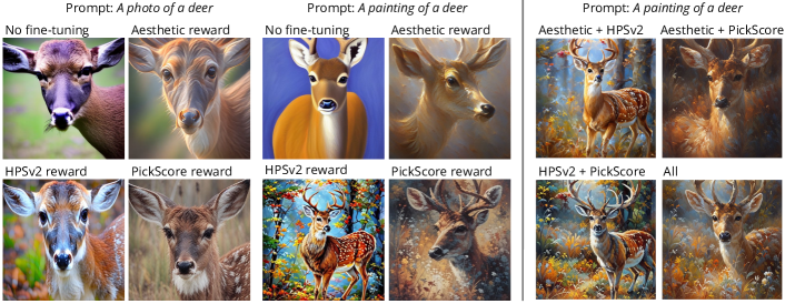
First, we trained DRaFT models using the aesthetic, PickScore, and HPSv2 rewards on the same set of 45 animal prompts. As the reward models behave differently for photographs and paintings, we trained two versions of each model. Qualitatively, we found the different reward functions led to quite different generated images (see Figure 5, right). HPSv2 generally encourages more colorful but less photo-realistic generations.

Figure 5: Left: Comparison of generations (using the same random seed) from DRaFT models fine-tuned on the LAION Aesthetic Classifier, Human Preference Score v2, and PickScore reward functions. Right: Outputs of DRaFT models combined by mixing the LoRA weights.

Figure 6: A DRaFT model trained on a simple prompt set of 45 animals generalizes well to other image subjects while preserving the learned style (Human Preference Score v2 reward).

Human Preference Score Comparison.

Next, we compared DRaFT-finetuned models to several baselines on the Human Preference Score v2 benchmark (Wu et al., 2023a). This benchmark consists of four prompt categories, {Animation, Concept Art, Paintings, Photos}, each with 800 prompts. We used DRaFT to fine-tune for HPSv2, using the Human Preference Dataset v2 (HPDv2) traning set prompts. In Figure 4, we report the mean performance over the four test set categories; Table 2 in Appendix B.2 provides a detailed breakdown of results by category. We compared DRaFT to a selected set of baselines from Wu et al. (2023a), as well as to DOODL (Wallace et al., 2023) and ReFL (Xu et al., 2023). As ReFL does not use guidance during training, we also experimented with adding guidance to it. Interestingly, the model with guidance performs similarly; possibly fine-tuning compensates for the lack of guidance similarly to how guided diffusion models can be distilled into unguided ones (Meng et al., 2023). DRaFT-1 slightly outperforms ReFL, while being simpler to implement. DRaFT-LV achieves the best reward value, learning approximately $2\times$ faster than DRaFT-1 (see the “DRaFT-LV, 5k steps” bar). Figure 4 also provides an ablation comparing DRaFT-$K$ for $K\in\{1,5,10,30,50\}$. Interestingly, we found that using smaller $K$ was beneficial, both in terms of training time and final performance.

Evaluating Generalization.

Next, we investigated several types of generalization: 1) prompt generalization, where we fine-tune for HPSv2 on one prompt dataset (Pick-a-Pic) and evaluate performance on another prompt dataset (HPDv2)—these results are shown by the “DRaFT, Pick-a-Pic” bars in Figure 4; and 2) reward generalization, where we fine-tune using a different reward (PickScore) than we use for evaluation (HPSv2)—these results are shown by the “DRaFT, PickScore” bars. DRaFT-1 and DRaFT-LV transfer well across prompt sets and fairly well across reward functions. We also show qualitative prompt generalization results in Figure 6: we found that a model fine-tuned using only 45 animal prompts learns a style that generalizes well to other prompts.

Large-Scale Multi-Reward Model.

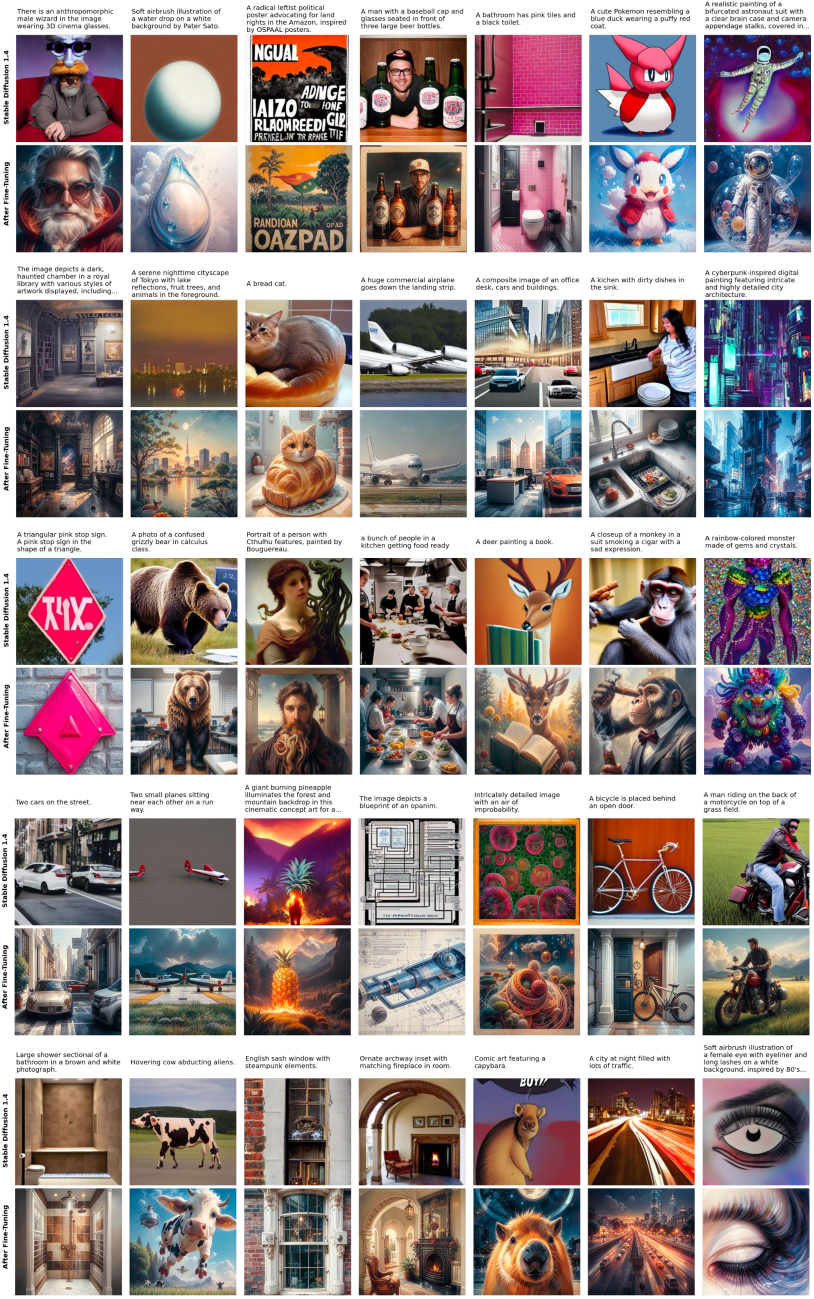
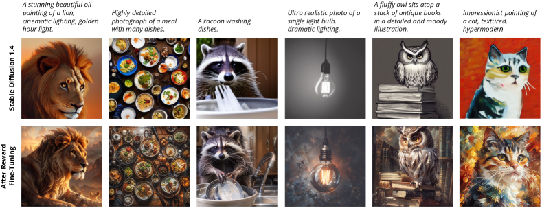
We pushed the scale of DRaFT-LV further by performing a 2x longer training run on the larger PickScore dataset, optimizing for a weighted combination of rewards, $\text{PickScore}=10,\text{HPSv2}=2,\text{Aesthetic}=0.05$. Images generated by the model are shown in Figure 1. Overall, the fine-tuned model produces more detailed and stylized images than baseline stable diffusion. In some cases, fine-tuning improves the model’s image-text alignment as well as aesthetics, because the PickScore and HPSv2 rewards measure the similarity between the prompt and image embeddings. For example, the model almost always generates images faithful to the prompt “a raccoon washing dishes,” while baseline stable diffusion does so less than half the time. However, we also found that the model sometimes overgeneralizes the reward function, generating detailed images even when the prompt calls for a simpler style (see Figure B.1 in Appendix B).

Figure 7: Interpolating LoRA parameters. Left: Generations from DRaFT models with different scalar multipliers applied to the LoRA weights. Scaling LoRA parameters yields semantic interpolations between the pre-trained and fine-tuned models. Right: Combining LoRA parameters that have been tuned independently for two different rewards—PickScore and HPSv2—allows for fine-grained control over style without additional training. For a fixed noise sample, we show images generated using $\alpha{\bm{\theta}}^{\text{PickScore}}_{\text{LoRA}}+\beta{\bm{\theta}}^{\text{HPSv2}}_{\text{LoRA}}$.

Scaling and Mixing LoRA Weights.

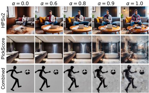
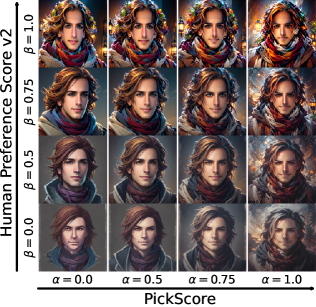
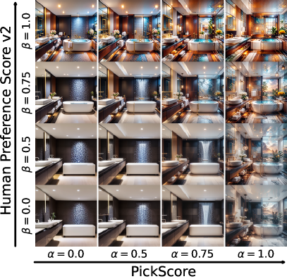
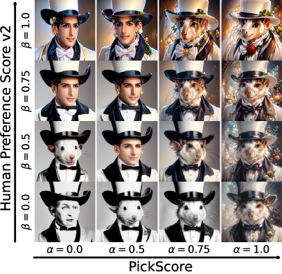
We show it is possible to control the strength of the fine-tuning simply by scaling the LoRa weights: multiplying the LoRA parameters by a scalar $\alpha<1$ moves the adapted parameters closer to the original, pre-trained model. Figure  7 (Left) shows that this method smoothly interpolates between the pre-trained and DRaFT models. The LoRA scale could become a useful hyperparameter for controlling generations from DRaFT models similar to how the guidance strength is currently used. We also probe the compositional properties of LoRA weights adapted for different rewards. One can combine the effects of reward functions by summing the LoRA weights of the respective DRaFT models (Figure 5, Left). In Figure 7 (Right), we show images generated using linear combinations of LoRA parameters trained separately for the PickScore and HPSv2 rewards, using scaling coefficients $\alpha$ and $\beta$. The resulting images mix the semantics of HPSv2 and PickScore, and are simultaneously more saturated and detailed than the pre-trained model outputs. The idea of combining LoRA weights is similar to model soups (Wortsman et al., 2022), and has been explored in NLP by Huang et al. (2023) and Zhang et al. (2023). While it would also be possible to instead directly sum the score functions of the models (similar to Liu et al. 2022), this would increase generation time proportional to the number of combined models.

Understanding the Impact of $K$.

Figure 8: Gradient norms

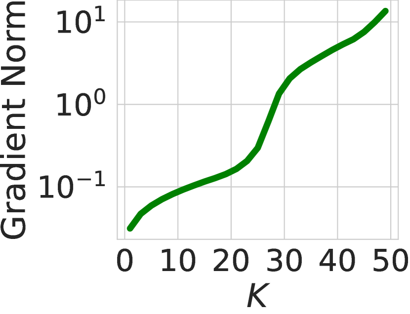
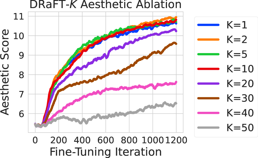
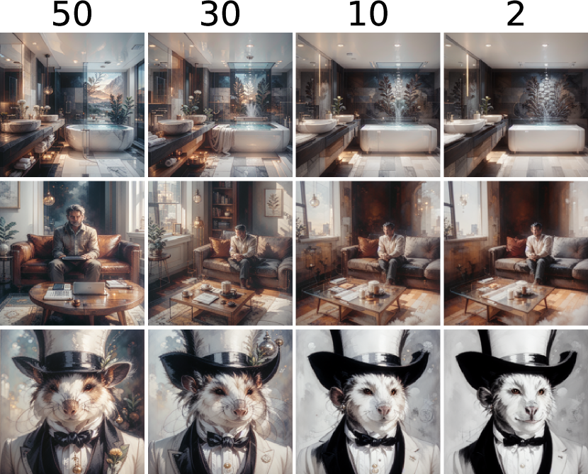
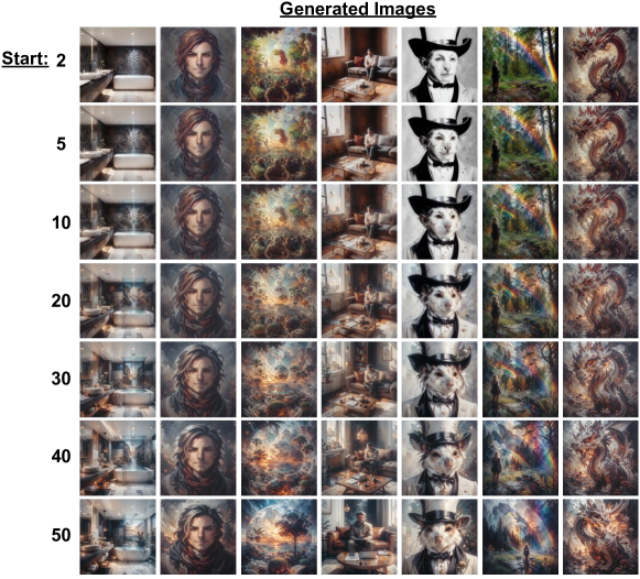
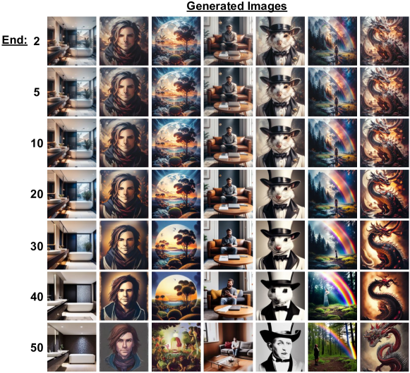
Interestingly, we found that truncated backpropagation improves sample efficiency as well as compute efficiency. Our initial analysis suggests that gradients explode as $K$ increases, which may lead to optimization difficulties for large $K$ (see Figure 8). In Figure 10, we show an ablation over $K$ for aesthetic fine-tuning: performance degrades as $K$ increases for $K>10$. In Figure 10, we show that although DRaFT-1 only computes gradients through the final generation step, it generalizes across time and affects the whole sampling chain. We compare samples generated with different LoRA start iterations $M$, where we applied the LoRA-adapted diffusion parameters for the last $M$ steps of the sampling chain, while in the first $T-M$ steps we used the pre-trained Stable Diffusion parameters without LoRA adaptation. We observe that adaptation does not happen only at the end of sampling (also see Figure 26 in App. B.7). We also investigated the opposite scenario, where the LoRA-adapted parameters are used in the first $M$ steps, after which LoRA is “turned off” and we use only the original pre-trained parameters for the remaining $T-M$ steps (see Figure 27 App. B.7), which shows that it is also important to apply the LoRA parameters early in sampling.

Figure 9: Ablation over $K$ for aesthetic reward fine-tuning.

Figure 10: Images generated with different LoRA start steps $M\in\{50,30,10,2\}$.

5.3 Other Reward Functions

Here, we show that DRaFT can be applied to diverse reward functions.

Compressibility and Incompressibility.

Figure 11: Top: Images generated by a diffusion model fine-tuned for JPEG compressibility, with reward $r(\mathbf{x}_{0})=-\|\mathbf{x}_{0}-d(c(\mathbf{x}_{0}))\|_{2}^{2}$ where $\mathbf{x}_{0}=\text{sample}({\bm{\theta}},\mathbf{c},\mathbf{x}_{T})$. Bottom: Using the negation of the compressibility loss yields images that are difficult to compress.

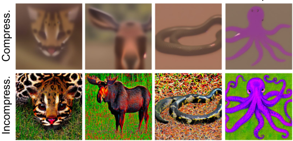
Inspired by Black et al. (2023), we also fine-tuned a diffusion model to generate easily-compressible images. While the JPEG compression and decompression algorithms available in common libraries are not differentiable by default, they can be implemented in a differentiable manner using deep learning libraries like PyTorch (Paszke et al., 2019) or JAX (Bradbury et al., 2018). Given a prompt $\mathbf{c}$, we pass the output of the diffusion model, $\mathbf{x}_{0}=\text{sample}({\bm{\theta}},\mathbf{c},\mathbf{x}_{T})$ through differentiable compression and decompression algorithms to obtain $d(c(\mathbf{x}_{0}))$, and minimize the Euclidean distance between the original and reconstructed images. This encourages the diffusion model to produce simple images. The results using DRaFT to fine-tune for JPEG compressibility are shown in Figure 11 (Top): these images have simple, uniform-color backgrounds and low-frequency foregrounds. In addition, negating the compressibility loss yields incompressible images, shown in Figure 11 (Bottom), that have complex, high-frequency foregrounds and backgrounds. Additional details are provided in App. B.3.

Object Detection and Removal.

Figure 12: Fine-tuning for object removal or addition using the OWL-ViT object detector. Left: The prompt to the diffusion model is a farmer market and the queries for OWL-ViT are $\mathcal{Q}=\{\text{{a person}, {people}}\}$. Before fine-tuning, most of the generated images contain people in the background; after finetuning, all images contain only vegetables. Right: Adding strawberries to a fruit bowl.

Here, we explore the use of a pre-trained object detection model to bias a diffusion model’s generations to include or exclude a certain object class. We use OWL-ViT (Minderer et al., 2022), an open-world localization model that takes arbitrary text queries and returns bounding boxes with scores for the corresponding objects in the image. We pass images generated by the diffusion model through a pre-trained OWL-ViT model, together with a set of queries $\mathcal{Q}$ that we wish to exclude from the generated images (see Figure 22 in Appendix B.6 for details). As the reward, we use the sum of scores for the localized objects corresponding to all queries $q\in\mathcal{Q}$, as well as the areas of their bounding boxes. In Figure 12 (Left), we show the results of fine-tuning to minimize detection of people. Similarly, we can maximize the sum of scores for localized objects to encourage generations to include a certain class: in Figure 12 (Right), we use the prompt “a bowl of fruit” and queries $\mathcal{Q}=\{\text{strawberry}\}$.

Adversarial Examples.

Figure 13: Diffusion adversarial examples for prompts bear, dog, mouse with target class cat.

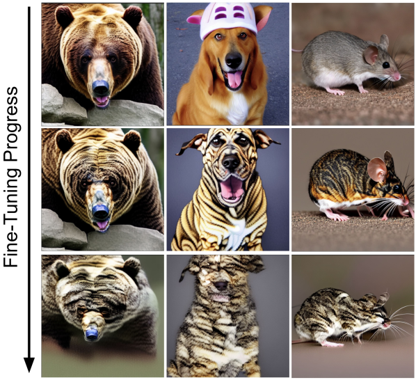
Our framework also provides an avenue to study the inductive biases of both diffusion models and pre-trained classifiers: we can fine-tune a diffusion model such that images generated based on a prompt for a class $y$ (e.g., “mouse”) are classified as a different class $y^{\prime}$ (e.g., “cat”) by a ResNet-50 pretrained on ImageNet. As the fine-tuning reward, we use the negative cross-entropy to the target class. From the qualitative results shown in Figure 13, we observe that this classifier is texture-biased (Geirhos et al., 2019), as the images generated by the fine-tuned model incorporate cat-like textures while keeping the animal shapes mostly unchanged.

6 Conclusion

We introduced an efficient framework for fine-tuning diffusion models on differentiable rewards by leveraging reward gradients. Our first method, Direct Reward Fine-Tuning (DRaFT), backpropagates through the full sampling procedure, and achieves strong performance on a variety of reward functions. We then propose DRaFT-$K$ and DRaFT-LV, variants which improve efficiency via truncated backpropagation through time. In addition, we draw connections between our approach and prior work such as ReFL (Xu et al., 2023), to provide a unifying perspective on the design space of gradient-based reward fine-tuning algorithms. We show that various methods can be obtained as special cases of a more general algorithm, depending on the whether—and where—stop_gradient operations are included. We hope that our work will inspire the development of improved techniques for reward fine-tuning; just as RLHF has become crucial for deploying large language models, we believe that reward fine-tuning may become a key step for improving image generation models.

Appendix

This appendix is structured as follows:

• In Appendix A, we provide more details of our experimental setup, including hyperparameters and baselines.

• In Appendix B, we provide additional results and analysis.

• In Appendix C, we discuss two other methods we explored that did not achieve as strong results as DRaFT-LV: a single-reward version of DRaFT-LV and applying Deterministic Policy Gradient.

• In Appendix D, we provide an extended discussion of related work.

• In Appendix E, we provide un-curated samples from models fine-tuned for various reward functions, including HPSv2, PickScore, and a combined reward weighting HPSv2, PickScore, and Aesthetic score.

Appendix A Experimental Setup

A.1 Additional Experimental Details and Hyperparameters

Here we expand on training details and list hyperparameters. We use the same hyperparameters for ReFL and our DRaFT variants.

Optimization.

We use the AdamW optimizer (Loshchilov & Hutter, 2019) with $\beta_{1}=0.9$, $\beta_{2}=0.999$, and a weight decay of 0.1. As we use LoRA, the weight decay regularizes fine-tuning by pushing parameters towards the pre-trained weights. For the longer training runs (10k steps on human preference reward functions), we use a square root learning rate decay, scaling the learning rate by $\min{(10\cdot\text{step}^{-0.5},1)}$. Weight decay and learning rate decay slightly improve results, but are not critical to the method. During training, we convert the pre-trained Stable Diffusion parameters to bfloat16 to reduce the memory footprint, but use float32 for the LoRA parameters being trained.

LoRA.

We apply LoRA to the feedforward layers as well as the cross-attention layers in the UNet, which we found to produce slightly better results. We apply LoRA only to the UNet parameters, not to the CLIP text encoder or VAE decoder mapping latents to images, as these did not improve results in initial experiments.

Sampling.

We use 50 steps of DDIM sampling (where no noise is added during sampling beyond the initial sampled noise). We found results using ancestral/DDPM sampling to be similar. We employ classifier-free guidance with a guidance weight of 7.5 both at train-time and test-time.

Hyperparameters.

We apply DRaFT in two settings: large-scale (human preference reward functions using the HPSv2 or PickScore prompt sets) and small-scale (the other experiments). Hyperparameters are listed in Table 1. Small-scale training runs take around 1.5 hours on 4 TPUv4s. Large-scale training runs take around 8 hours on 16 TPUv4s.

Hyperparameter	Small-Scale Experiments	Large-scale Experiments
Learning rate	4e-4	2e-4
Batch size	4	16
Train steps	2k	10k
LoRA inner dimension	8	32
Weight decay	0.1	0.1
DDIM steps	50	50
Guidance weight	7.5	7.5
DRaFT-LV inner loops $n$	2	2
ReFL max timestep $m$	20	20

Table 1: Training hyperparameters.

A.2 Reward Function Details

The LAION aesthetic predictor is trained to rate images on a scale of 1 through 10. The predictor consists of a feedforward neural network on top of a CLIP (Radford et al., 2021) image encoder pre-trained on a variety of human-labeled sources.

Human Preference Score v2 (HPSv2; Wu et al. 2023a) is trained on prompts from DiffusionDB (Wang et al., 2023) and COCO Captions (Chen et al., 2015). Images are generated from each using a wide range of generative models. Human annotators then rate which of two images is preferred for a prompt. The reward model is OpenCLIP-H (Beaumont et al., 2022) fine-tuned on the preference judgements. Unlike the aesthetic reward, HPSv2 takes into account the prompt as well as the image.

PickScore (Kirstain et al., 2023) also uses OpenCLIP-H fine-tuned on preference data. However, the data is collected in a more organic way through a web app, where users can generate and then rate pairs of images generated from different diffusion models with different sampler hyperparameters.

A.3 Baselines

Denoising Diffusion Policy Optimization (DDPO; Black et al. 2023) essentially applies the REINFORCE policy gradient algorithm (Williams, 1992) to diffusion model generation. The method trains the model to increase the likelihoods of actions (i.e. sampling steps) that produce high-reward samples. DDPO employs additional tricks such as importance weight clipping, reward normalization, and classifier-free guidance-aware training to improve results. We show results from DDPO-IS, which extends DDPO to use an importance sampling estimator for learning on examples generated from a stale policy, enabling multiple optimization updates per reward query. Empirically, DDPO was found to outperform previous supervised approaches like reward weighted regression (Lee et al., 2023). Rather than using the results in Figure 4 of the original paper, we obtained results from direct correspondence with the authors, as their original aesthetic reward implementation had a bug.

Prompt Engineering.

Users often improve the aesthetic quality of generated images through prompt engineering. We perform semi-automated prompt search with access to the reward function, trying out various prompts and selecting the one with the best aesthetic score. The best-scoring prompt we found is A stunning beautiful oil painting of a {:}, cinematic lighting, golden hour light.

Re-ranking (Best of 16).

This simple baseline generates 16 images for each caption with the pre-trained stable diffusion model and selects the one with the highest reward.

Direct Optimization of Diffusion Latents (DOODL).

DOODL (Wallace et al., 2023) backpropagates through diffusion sampling to update the initial noise $\mathbf{x}_{T}$ so that the resulting generation produces a high reward. Rather than using an invertible diffusion algorithm to reduce memory costs as in Wallace et al. (2023), we simply use gradient checkpointing as with DRaFT. We optimize $\mathbf{x}_{T}$ with Adam (which worked slightly better for us than momentum only) over 20 steps, which makes generation approximately 60x lower than standard sampling. Following Wallace et al. (2023), we renormalize the latent at every step after the Adam update.

Appendix B Additional Experimental Results

B.1 Over-generalization

Here we show examples of overgeneralization, where fine-tuning on preferences trains the model to generate detailed images, even when the prompt asks for a simple drawing.

B.2 Full Quantitative Results

In Table 2, we provide quantitative results comparing DRaFT to several baselines on the Human Preference Score v2 benchmark from Wu et al. (2023a).

Model	Animation	Concept Art	Painting	Photo	Averaged
GLIDE 1.4	$0.2334$	$0.2308$	$0.2327$	$0.2450$	$0.2355$
VQGAN + CLIP	$0.2644$	$0.2653$	$0.2647$	$0.2612$	$0.2639$
DALL-E 2	$0.2734$	$0.2654$	$0.2668$	$0.2724$	$0.2695$
SD 2.0	$0.2748$	$0.2689$	$0.2686$	$0.2746$	$0.2717$
DeepFloyd-XL	$0.2764$	$0.2683$	$0.2686$	$0.2775$	$0.2727$
SDXL Base 0.9	$0.2842$	$0.2763$	$0.2760$	$0.2729$	$0.2773$
Dreamlike Photoreal 2.0	$0.2824$	$0.2760$	$0.2759$	$0.2799$	$0.2786$
Stable Diffusion (SD 1.4)	$0.2726$	$0.2661$	$0.2666$	$0.2727$	$0.2695$
ReFL	$0.3446$	$0.3442$	$0.3447$	$0.3374$	$0.3427$
DRaFT-50	$0.3078$	$0.3021$	$0.3019$	$0.3013$	$0.3033$
DRaFT-30	$0.3148$	$0.3112$	$0.3109$	$0.3096$	$0.3116$
DRaFT-10	$0.3456$	$0.3447$	$0.3452$	$0.3369$	$0.3431$
DRaFT-5	$0.3521$	$0.3520$	$0.3526$	$0.3431$	$0.3500$
DRaFT-1	$0.3494$	$0.3488$	$0.3485$	$0.3400$	$0.3467$
DRaFT-1, PickScore	$0.2907$	$0.2848$	$0.2861$	$0.2882$	$0.2875$
DRaFT-1, Pick-a-Pic	$0.3399$	$0.3358$	$0.3385$	$0.3188$	$0.3332$
DRaFT-LV	$0.3551$	$0.3552$	$0.3560$	$0.3480$	$0.3536$
DRaFT-LV, PickScore	$0.2880$	$0.2833$	$0.2846$	$0.2923$	$0.2870$
DRaFT-LV, Pick-a-Pic	$0.3409$	$0.3371$	$0.3408$	$0.3210$	$0.3349$

Table 2: Following Wu et al. (2023a), we use the HPDv2 training set to fine-tune our models, and we evaluate performance on four benchmark datasets: Animation, Concept Art, Paintings, and Photos. We report the average score achieved for each benchmark, as well as the aggregated performance across all datasets. The results above the separator are taken from Wu et al. (2023a); the results below were obtained from our implementations and experiments.

B.3 Compressibility and Incompressibility Details

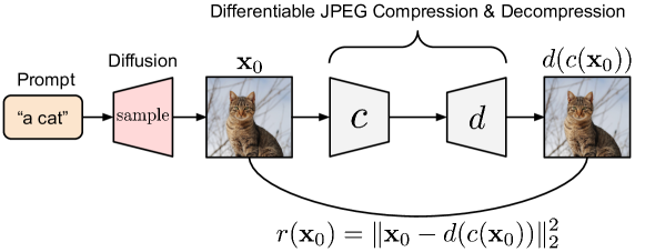
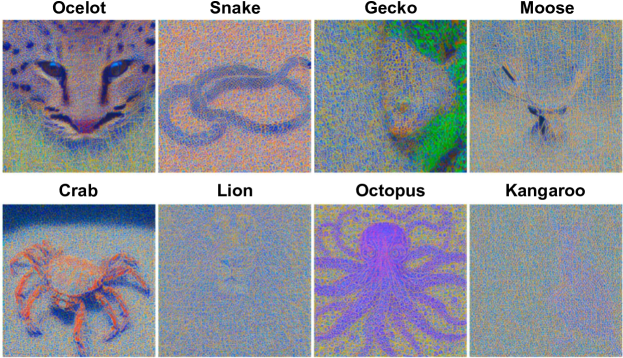
Figure 14 illustrates the setup we used to fine-tune for JPEG compressibility and incompressibility. Given a prompt $\mathbf{c}$, we take the image generated by the diffusion model, $\mathbf{x}_{0}=\text{sample}({\bm{\theta}},\mathbf{c},\mathbf{x}_{T})$ and pass it through JPEG compression and decompression functions, denoted by $c$ and $d$, respectively. As the reward, we use the negative Euclidean distance between the original sample $\mathbf{x}_{0}$ and its reconstruction $r(\mathbf{x}_{0})=-\|\mathbf{x}_{0}-d(c(\mathbf{x}_{0}))\|^{2}$. While the JPEG implementations found in common libraries are not directly differentiable, the JPEG algorithm can be re-implemented in a differentiable way using autodiff frameworks; we re-implemented JPEG compression and decompression in JAX (Bradbury et al., 2018). Figures 15 and 16 show additional samples generated by diffusion models fine-tuned for compressibility and incompressibility, respectively, and Figure 17 shows the results of overoptimization for incompressibility. In our experiments, we used a fixed compression ratio of $4\times$.

Figure 14: Fine-tuning for JPEG compressibility, using differentiable JPEG compression and decompression algorithms.

Figure 15: Images generated by a diffusion model fine-tuned for JPEG compressibility.

Figure 16: Images generated by a diffusion model fine-tuned using the negation of the JPEG compressibility reward, which yields images that are difficult to compress. We observe high-frequency foreground and background information.

Figure 17: Over-optimization for JPEG incompressibility can lead to images with strong high-frequency texture and a loss of semantic information. Interestingly, here the octopus is generated with more than eight arms.

B.4 Adversarial Example Details

The setup for our diffusion adversarial example experiments is illustrated in Figure 18. We used a ResNet-50 model pre-trained on ImageNet-1k to classify images generated by Stable Diffusion; as the reward for fine-tuning, we used the negative cross-entropy to a fixed target class.

Figure 18: Generating “diffusion adversarial examples” that are conditioned on a text prompt (e.g., “mouse”) but must be classified by a pre-trained ImageNet classifier as a different class (e.g., “cat”).

B.5 LoRA Scaling and Interpolation

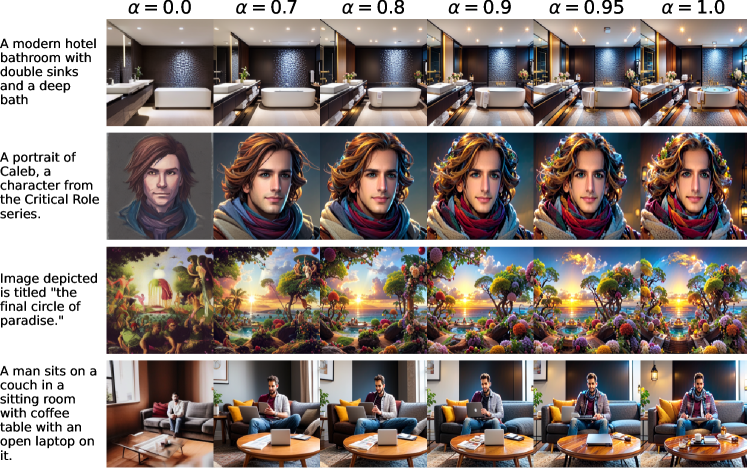
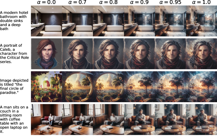
Here, we provide additional results for scaling and interpolating LoRA parameters. Figures 19 and 20 show the effect of scaling LoRA parameters to control the strength of reward adaptation for the Human Preference Score v2 and PickScore rewards, respectively, and Figure 21 shows additional interpolations using linear combinations of LoRA weights trained separately for each of these rewards.

Figure 19: Scaling LoRA parameters (here adapted for Human Preference Score v2 (Wu et al., 2023a)) yields semantic interpolations between the original Stable Diffusion model and the fine-tuned model.

Figure 20: Scaling LoRA parameters (here adapted for PickScore (Kirstain et al., 2023)) yields semantic interpolations between the original Stable Diffusion model and the fine-tuned model.

Figure 21: Additional results using linear combinations of LoRA parameters adapted for different rewards. In each subplot, we show images generated using parameters ${\bm{\theta}}+\alpha{\bm{\theta}}^{\text{PickScore}}+\beta{\bm{\theta}}^{\text{HPSv2}}$ for coefficients $\alpha,\beta\in\{0.0,0.5,0.75,1.0\}$. We found that interpolating between LoRA weights can smooth transitions between different styles.

B.6 Object Detection

Figure 22: Fine-tuning for object detection using a pre-trained OWL-ViT model (Minderer et al., 2022).

Figure 23: Maximizing the object detector score for the query “strawberry” yields fruit bowls that contain progressively more strawberries over the course of fine-tuning.

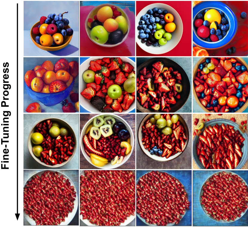
Our setup for object detection is illustrated in Figure 22. We feed the generated images into a pre-trained Open-World Localization Vision Transformer (OWL-ViT) (Minderer et al., 2022) model, along with a list of text queries that we wish to localize in the image. OWL-ViT outputs bounding boxes and scores for the localized objects; we experimented with reward functions based on the sum of scores, as well as based on the areas of the bounding boxes, and found that both worked well. Figure 23 shows the fine-tuning progress for the diffusion prompt “a bowl of fruit” with OWL-ViT query “strawberries.”

B.7 Understanding the Impact of $K$

We investigated the impact of $K$ on the behavior of models fine-tuned with DRaFT-$K$ via ablations designed to answer the following questions: 1) Does adaptation occur only in the last $K$ steps (e.g., does the initial segment of the sampling chain behave similarly to the original pre-trained model, with a sudden jump occurring at the end)? and 2) Is it necessary to apply the LoRA parameters throughout the full sampling chain? What is the impact of applying the LoRA parameters to only the initial or final portions of the trajectory?

Figure 24: Angles between the DRaFT-1 gradient and DRaFT-$K$ gradients for $K\in\{1,\dots,50\}$.

To answer these questions, we applied the LoRA-adapted diffusion parameters for the last $M$ steps of the sampling chain, while in the first $T-M$ steps we used the pre-trained Stable Diffusion parameters without LoRA adaptation (see Figure 25). Figure 26 compares samples generated with different LoRA start iterations $M$; interestingly, although the LoRA parameters are fine-tuned using truncated backpropagation through only the last $K$ steps of sampling, adaptation does not happen only in the last $K$ steps; rather, the LoRA parameters need to be applied for at least 10-20 steps to yield substantial changes in the generated images. Similarly, we also investigated the opposite scenario, where the LoRA-adapted parameters are only applied in the first $M$ steps of the sampling chain, after which LoRA is “turned off” and we use only the original pre-trained parameters for the remaining $T-M$ steps. The generated images for a range of end LoRA steps $M\in\{2,5,10,20,30,40,50\}$ are shown in Figure 27. These results further demonstrate the importance of applying LoRA parameters in the early part of the sampling chain.

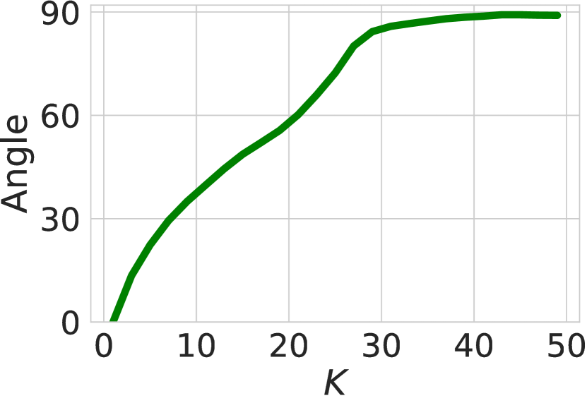
In Figure 24, we show the angle between the DRaFT-1 gradient and DRaFT-$K$ gradients for various $K$; the gradients become nearly orthogonal for $K>30$.

Figure 25: Illustration of sampling with different LoRA start steps and end steps.

Figure 26: Images generated with different LoRA start steps. Here, the first $T-M$ steps of the diffusion sampling chain use the pre-trained diffusion model parameters, while the last $M$ steps use the LoRA-adapted parameters. The LoRA start step $M$ increases from top to bottom, $M\in\{2,5,10,20,30,40,50\}$. We observe that, although the LoRA parameters are trained via truncated backpropagation through the last few steps of sampling, they affect the entire sampling chain—the images improve qualitatively when the LoRA-adapted parameters are used for many steps (e.g., $M>10$).

Figure 27: Images generated with different LoRA “end steps.” Here, the first $M$ steps of the diffusion sampling chain use the LoRA-adapted diffusion parameters, while the last $T-M$ steps use the un-adapted pre-trained model parameters. The LoRA end step $M$ increases from top to bottom, $M\in\{2,5,10,20,30,40,50\}$. Interestingly, we observe that it is beneficial to apply the LoRA parameters early in sampling.

Figure 28: Reward hacking still occurs when we use large dropout rate in the Aesthetic classifier (Left). Incorporating a reward term to encourage diversity can lead to overly stylized images (Right).

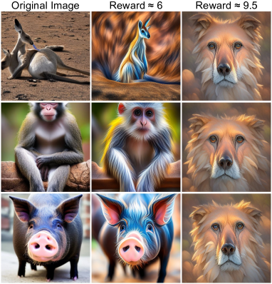
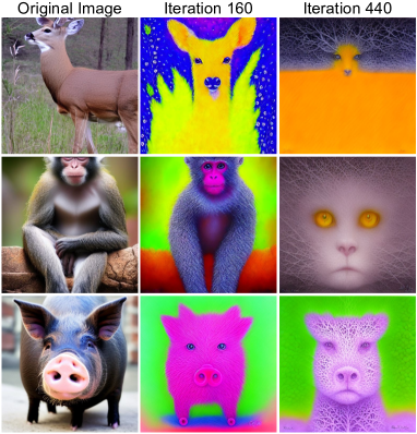
B.8 “Over-Optimization” and Reward Hacking

Attempts to Increase Diversity.

A common result of reward hacking is a collapse to a single, high-reward image. Here, we describe two of our attempts to address this lack of diversity. First, we tried adding dropout to the reward function (in this case, the aesthetic classifier); however, we found that even large dropout rates such as 0.95 led to diversity collapse, as shown in Figure 28 (Left). Next, we tried adding a term to the reward that measures the dissimilarity between images generated in the same minibatch—this encourages the model to generate different images for different prompts and noise samples. Ideally, one would take the mean dissimilarity over all pairs of examples in a minibatch, yielding $B\choose 2$ combinations where $B$ is the minibatch size. However, for computational tractability, we used a simpler approach, where we form pairs by reversing the elements of a minibatch and computing elementwise dissimilarities, giving us $B/2$ pairs. We tried two measures of dissimilarity: 1) the Euclidean distance, and 2) the Learned Perceptual Image Patch Similarity (LPIPS) (Zhang et al., 2018). Neither was satisfactory to increase diversity: in Figure 28 (Right), we show images generated using a large weight on the LPIPS diversity term, which increased inner-batch diversity at the expense of the aesthetic score.

B.9 Rotational Anti-Correlation Reward

Figure 29: Rotational anti-correlation.

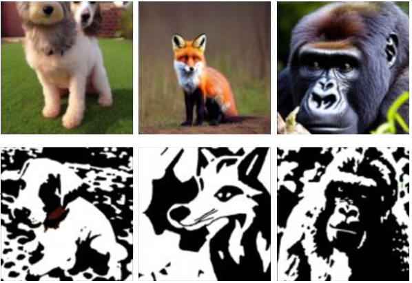
We also explored fine-tuning for symmetry or anti-symmetry properties. Here, we optimize for rotational anti-correlation, which encourages the diffusion model to generate images that are dissimilar to their rotations at $\{90,180,270\}$ degrees. Given an image $\mathbf{x}$ and rotation operator $\text{Rot}(\mathbf{x},90^{\circ})$, we formulate the objective as: $\mathbb{E}_{\mathbf{c}\sim p_{\mathbf{c}},\mathbf{x}\sim\text{sample}({\bm{\theta}},\mathbf{c})}\Big{[}\frac{1}{3}\Big{(}\|\mathbf{x}-\text{Rot}(\mathbf{x},90^{\circ})\|^{2}+\|\mathbf{x}-\text{Rot}(\mathbf{x},180^{\circ})\|^{2}+\|\mathbf{x}-\text{Rot}(\mathbf{x},270^{\circ})\|^{2}\Big{)}\Big{]}$. The results are shown in Figure 29: this objective leads to interesting black-and-white, stylized images.

B.10 CLIP Reward

We briefly explored using $r(\mathbf{x}_{0},\mathbf{c})=\text{CLIP-Similarity}(\mathbf{x}_{0},\mathbf{c})$ as a reward to improve image-text alignment. We found that optimization was succesful in that CLIP scores improved, but that image quality degraded after many steps of training (see Figure 30).

Figure 30: Qualitative examples (left) and training curve (right) for fine-tuning on CLIP reward using DRaFT for the prompt “a racoon washing dishes".

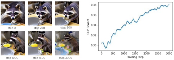
Both HPSv2 and ImageReward are fine-tuned CLIP models, and for HPSv2 the annotators were specifically instructed to consider alignment to the prompt in their preference judgements. Therefore, they already capture some aspects of image alignment, and qualitatively we did observe alignment to increase in some cases when using these rewards (e.g. in the “a racoon washing dishes" example in Figure 1). However, we think improving text alignment using a powerful image captioning model such as PaLI (Chen et al., 2023) as the reward would be an interesting future direction.

B.11 Learning Sampler Hyperparameters

Figure 31: Guidance schedule learned by DRaFT

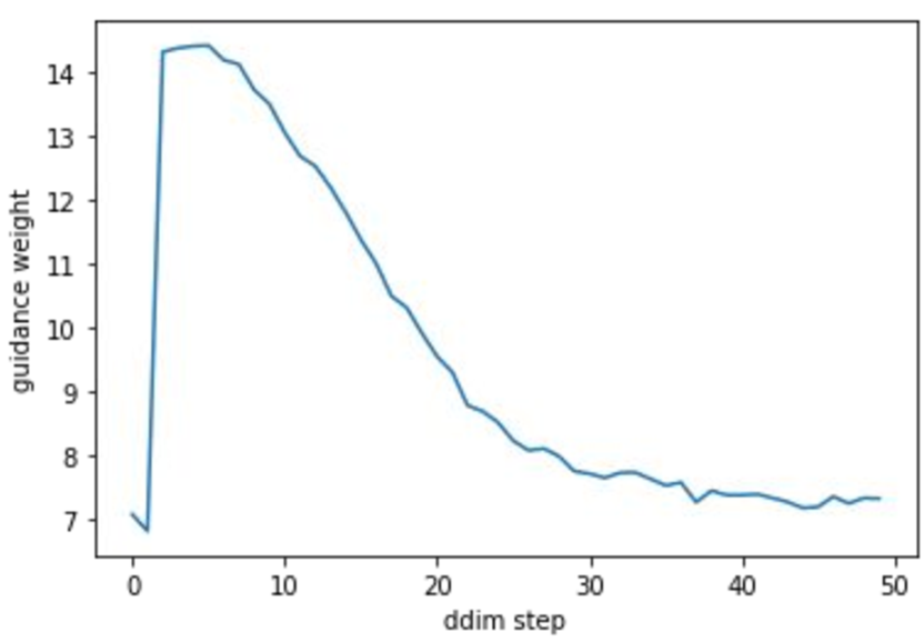
As DRaFT (without truncated backprop through time) computes gradients through the denoising process end-to-end, we can use DRaFT to optimize sampler hyperparameters as well as model weights.

Learning sampler hyperparameters is similar in spirit to Watson et al. (2021), except we obtain gradients from a reward model rather than using kernel inception distance. We explored learning two inputs to the sampler—the guidance weights and negative prompt embeddings—although it would be possible to extend this method to other hyperparameters such as the time schedule. In particular, we investigated:

• Guidance weights: We learn a separate guidance weight $w(t)$ for each step of DDIM sampling. The learned schedule can be applied to samplers with different number of steps through linearly interpolating the schedule to stretch or compress it. We use a 50x larger learning rate for training guidance than the LoRA parameters because guidance weights have a large magnitude. An example learned guidance schedule is shown in Figure 31.

• Negative prompt: We learn prompt-dependent text embeddings passed into the unconditional UNet used for classifier-free guidance. In particular, we parameterize the embedding as $\text{MLP}(\text{Multi-Headed-Self-Attention}(e))$ where $e$ is the text embeddings produced by the diffusion model’s text encoder.

However, in practice, we found that this did not improve results much at large scale.

Appendix C Method extensions

Here we briefly discuss two gradient-based reward fine-tuning methods we explored, but which we found did not achieve strong results compared to DRaFT-1 and DRaFT-LV.

C.1 Single-Reward DRaFT-LV

A downside of DRaFT-LV is that it requires computing the reward function gradient an additional $n$ times. While this is relatively little overhead for the reward functions we used compared to the cost of image sampling, larger reward models could make this costly. We therefore experimented with a version of DRaFT-LV that only computes the reward gradient with respect to the input pixels $\nabla_{\mathbf{x}}r(\mathbf{x}_{0},\mathbf{c})$ once. Then it updates the gradient in the inner loop as $\bm{g}=\bm{g}+\nabla_{\mathbf{x}}r(\mathbf{x}_{0},\mathbf{c})\nabla_{\bm{\theta}}\hat{\mathbf{x}}_{0}$. Unfortunately, we found this method to be unstable and ultimately not learn effectively, possibly because it relies on the assumption that $\nabla_{\mathbf{x}}r(\mathbf{x}_{0},\mathbf{c})\approx\nabla_{\mathbf{x}}r(\hat{\mathbf{x}}_{0},\mathbf{c})$, which may not be true in practice.

C.2 Deterministic Policy Gradient

Previous approaches applying RL to reward learning do not make use of sampling gradients. Here we discuss how Deterministic Policy Gradient (DPG; Silver et al. 2014; Lillicrap et al. 2016) offers a way of employing reward gradients within the RL framework.

Similar to Black et al. (2023), we can view DDIM sampling as applying a deterministic policy to a deterministic Markov decision process:

• A state $\mathbf{s}_{t}$ consists of the current latent, timestep, and prompt $(\mathbf{x}_{t},t,\mathbf{c})$.

• The initial state $\mathbf{s}_{0}$ draws $\mathbf{x}_{T}\sim\mathcal{N}(\bm{0},\mathbf{I}),\mathbf{c}\sim p_{\mathbf{c}}$, and sets $t=T$.

• The policy is the learned denoiser: $\mathbf{a}_{t}=\bm{\mu}_{\bm{\theta}}(\mathbf{s}_{t})=\bm{\epsilon}_{{\bm{\theta}}}(\mathbf{x}_{t},\mathbf{c},t)$

• The transition function performs a DDIM sampling step:
  $f(\mathbf{s}_{t},\mathbf{a}_{t})=(\frac{\alpha_{t-1}}{\alpha_{t}}(\mathbf{x}_{t}-\sigma_{t}\mathbf{a}_{t})+\sigma_{t-1}\mathbf{a}_{t},t-1,\mathbf{c})$

• The reward $R(\mathbf{s}_{t},\mathbf{a}_{t})$ is $r(\mathbf{x}_{0},\mathbf{c})$ if $t=0$ and 0 if otherwise.

DPG trains a critic $Q_{\bm{\phi}}(\mathbf{s}_{t},\mathbf{a}_{t})$ and learns ${\bm{\theta}}$ with the gradient update $\nabla_{\mathbf{a}}Q_{\bm{\phi}}(\mathbf{s}_{t},\mathbf{a}_{t})\nabla_{\bm{\theta}}\bm{\mu}_{\bm{\theta}}(\mathbf{s}_{t})$ over sampled trajectories. The critic is trained to minimize the squared error between its prediction and the final return (in our case $r(\mathbf{x}_{0},\mathbf{c})$).

Many of our reward make use of a neural network with pre-trained parameters $\bm{\xi}$, which we denote by writing $r_{\bm{\xi}}$. We suggest applying LoRA to $\bm{\xi}$ parameterize the critic; we denote the LoRA-adapted parameters as $\text{adapt}(\bm{\xi},\bm{\phi})$. We then apply the critic by (1) executing the action $\mathbf{a}_{t}$ on $\mathbf{s}_{t}$, (2) 1-step denoising the result to get a predicted clean image, and (3) applying the adapted reward model $r_{\text{adapt}(\bm{\xi},\bm{\phi})}$ to the result. The reason for step (2) is to make the training of $\bm{\phi}$ more efficient: we believe it is easier to adapt the reward model parameters to produce good expected return estimates for one-step-denoised inputs than it is for noisy inputs. Formally, we use the critic:

$$Q_{\bm{\phi}}(\mathbf{s}_{t},\mathbf{a}_{t})=r_{\text{adapt}(\bm{\xi},\bm{\phi})}((f(\mathbf{s}_{t},\mathbf{a}_{t})-\sigma_{t}\bm{\epsilon}_{{\bm{\theta}}}(f(\mathbf{s}_{t},\mathbf{a}_{t}),\mathbf{c},t-1))/\alpha_{t},\mathbf{c})$$ (3)

When computing gradients through $Q$, we do not backpropagate through step (2) into ${\bm{\theta}}$, to prevent it from interfering with the policy training.

Figure 32: Training efficiency of reward fine-tuning methods on the HPSv2 reward.

Results.

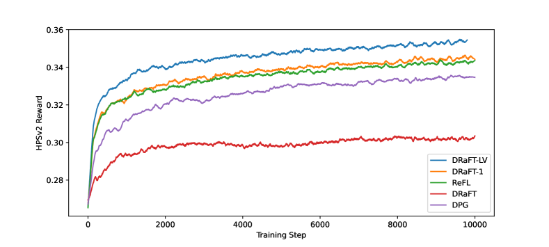
The training efficiency of DPG compared with other methods is shown in Figure 32 (using the same experimental settings as in Figure 4). DPG outperforms vanially DRaFT, but not our more-efficient variants. One challenge is that $Q$ produces poor return estimates for large timesteps, which could perhaps be alleviated with a ReFL-style version that skips or rarely samples high timesteps for training the policy. There are many variants of DPG to explore, so we think that improving the performance of DPG for reward fine-tuning could be an interesting direction for future research; DPG is appealing because like DRaFT (but unlike ReFL and our DRaFT variants), it optimizes the full sampling process in an unbiased way.

Appendix D Extended Related Work

Diffusion Models.

Denoising diffusion probabilistic models (DDPMs; Sohl-Dickstein et al. 2015; Song & Ermon 2019; Song et al. 2021b; Ho et al. 2020) are a class of generative models that have become the de-facto standard for most continuous data modalities, including images (Ramesh et al., 2021), videos (Ho et al., 2022; Singer et al., 2023), audio (Liu et al., 2023), and 3D models (Zeng et al., 2022; Poole et al., 2023; Gu et al., 2023). Text-to-image diffusion models, which generate images conditioned on text prompts, have become prominent tools with the advent of models such as GLIDE (Nichol et al., 2021), DALLE-2 (Ramesh et al., 2022), Imagen (Saharia et al., 2022; Ho et al., 2022), and Latent Diffusion (Rombach et al., 2022). In this paper we focus on fine-tuning text-to-image models, but DRaFT is general and could be applied to other diffusion models or fine-tuning tasks, and to different domains such as audio or video.

Learning human preferences.

Human preference learning trains models on judgements of which behaviors people prefer, rather than on human demonstrations directly (Knox & Stone, 2009; Akrour et al., 2011). This training is commonly done by learning a reward model reflecting human preferences and then learning a policy that maximizes the reward (Christiano et al., 2017; Ibarz et al., 2018). Preference learning methods such as reinforcement learning from human feedback (RLHF) have become widely used for fine-tuning large language models so they improve at summarization (Stiennon et al., 2020; Wu et al., 2021), instruction following (Ouyang et al., 2022), or general dialogue (Askell et al., 2021; Bai et al., 2022a; Glaese et al., 2022; Bai et al., 2022b). We apply DRaFT to optimize scores from existing preference models, such as PickScore (Kirstain et al., 2023) and Human Preference Score v2 (Wu et al., 2023a), which are trained on human judgements between pairs of images generated by diffusion models for the same prompt.

Guidance.

Guidance steers the sampling process towards images that satisfy a desired objective by adding an auxiliary term to the score function. The canonical example is classifier guidance (Song et al., 2021b; Dhariwal & Nichol, 2021), which can turn an unconditional diffusion model into a class-conditional model by biasing the denoising process using gradients from a pre-trained classifier. Many other pre-trained models can also be used to provide guidance signals, including segmentation models, facial recognition models, and object detectors (Bansal et al., 2023). However, care must be taken when computing the guidance signal; naïvely, noisy examples obtained during the iterative refinement process may be out-of-distribution for the guidance model, leading to inaccurate gradients. Two approaches for mitigating this are (1) training a guidance model from scratch on noisy data (Dhariwal & Nichol, 2021) and (2) applying a pre-trained guidance model (which has seen only non-noisy data) to the one-step-denoised images obtained by removing the predicted noise at time $t$ (Li et al., 2022). However, both approaches have downsides: (1) precludes the use of off-the-shelf pre-trained guidance functions and (2) means the guidance is applied to out-of-distribution blurry images for high noise levels. DRaFT avoids these issues by backpropagating through sampling so the reward function is only applied to the fully denoised image.

Backpropagation through diffusion sampling.

Similarly to our method, Watson et al. (2021) backpropagate through sampling using the reparameterization trick and gradient checkpointing. They learn parametric few-step samplers that aim to reduce the inference cost while maintaining perceptual image quality, using a differentiable image quality score. In contrast, we fine-tune the diffusion model parameters rather than the sampler to improve arbitrary differentiable rewards. Like DRaFT, Direct Optimization of Diffusion Latents (DOODL; Wallace et al. 2023) uses backpropagation through sampling to improve image generation with respect to differentiable objectives. Rather than optimizing model parameters, DOODL optimizes the initial noise sample $\mathbf{x}_{T}$. Although DOODL does not require a training phase, it is much slower at inference time because the optimization must be redone for each prompt and metric. In contrast, after finetuning with DRaFT, sampling has the same cost as a standard diffusion model. Furthermore, the latent optimization methods do not support the compositionality and interpolation properties that we can achieve with different sets of LoRA parameters tuned for different objectives.

Reward fine-tuning with supervised learning.

Lee et al. (2023) and Wu et al. (2023b) use supervised approaches to fine-tune diffusion models on rewards. These methods generate images with the pre-trained model and then fine-tune on the images while weighting examples according to the reward function or discarding low-reward examples. Unlike DRaFT or RL methods, the model is not trained online on examples generated by the current policy. However, Dong et al. (2023) use an online version of this approach where examples are re-generated over multiple rounds of training, which can be viewed as a simple kind of reinforcement learning.

Reward fine-tuning with reinforcement learning.

Black et al. (2023) and Fan et al. (2023) interpret the denoising process as a multi-step decision-making task, and use policy gradient algorithms to fine-tune diffusion models for arbitrary black-box objectives. Rather than optimizing model parameters, Hao et al. (2022) apply RL to improve the input prompts. RL approaches are flexible because they do not require differentiable rewards. However, in practice many reward functions are differentiable, or can be re-implemented in a differentiable way, and thus analytic gradients are often available. In such cases, using reinforcement learning discards useful information, leading to inefficient optimization.

ReFL.

Reward Feedback Learning (ReFL; Xu et al. 2023) evaluates the reward on the one-step predicted clean image, $r(\hat{\mathbf{x}}_{0},\mathbf{c})$ from a randomly-chosen step $t$ along the denoising trajectory, and backpropagates through the one-step prediction w.r.t. the diffusion model parameters.

DRaFT-$K$ is closely related to ReFL (Xu et al., 2023), but there are some important differences: 1) DRaFT-$K$ uses guidance during sampling, while the original ReFL algorithm did not—we found that using guidance helped to avoid degenerate solutions such as all generated images becoming identical. 2) DRaFT-$K$ is conceptually simpler, as it only differentiates through the last few steps (e.g., $K=2$) of sampling, where $K$ is deterministic; in (Xu et al., 2023), the authors randomly choose an iteration between a min and max step of the sampling chain (which incurs more hyperparameters) from which to predict the clean image. 3) Because we run the full sampling chain, our reward functions are always evaluated on final generations. In contrast, ReFL applies the rewards to one-step denoised latents in the sampling trajectory, similar to the use of one-step denoising in guidance. Furthermore, DRaFT-LV is substantially more efficient than ReFL, speeding up training by approximately 2x by reducing the variance of the single-denoising-step gradient estimates.

Appendix E Uncurated Samples

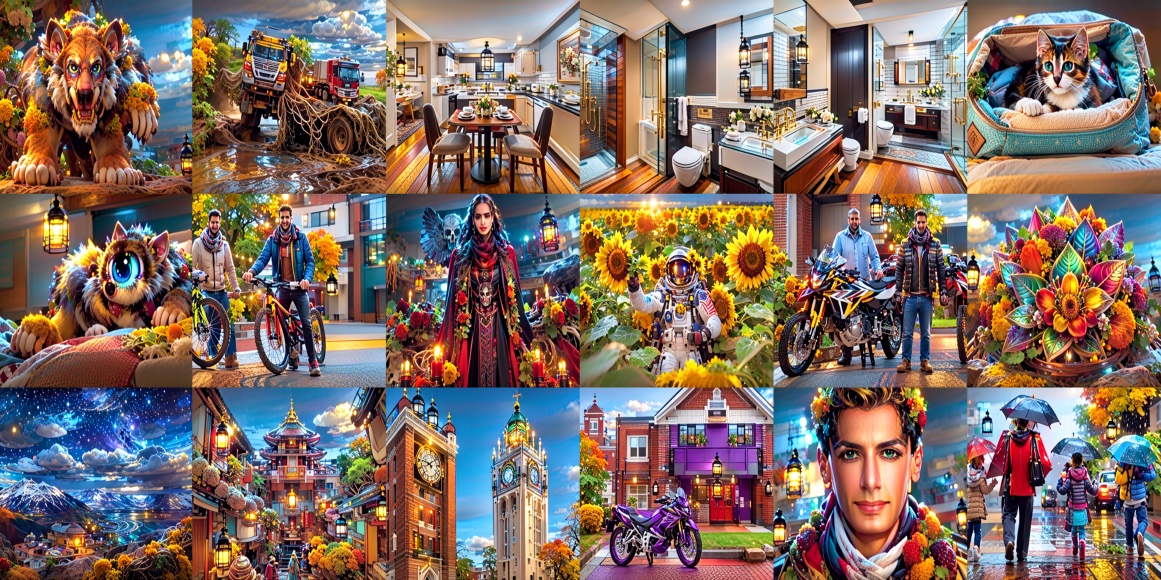
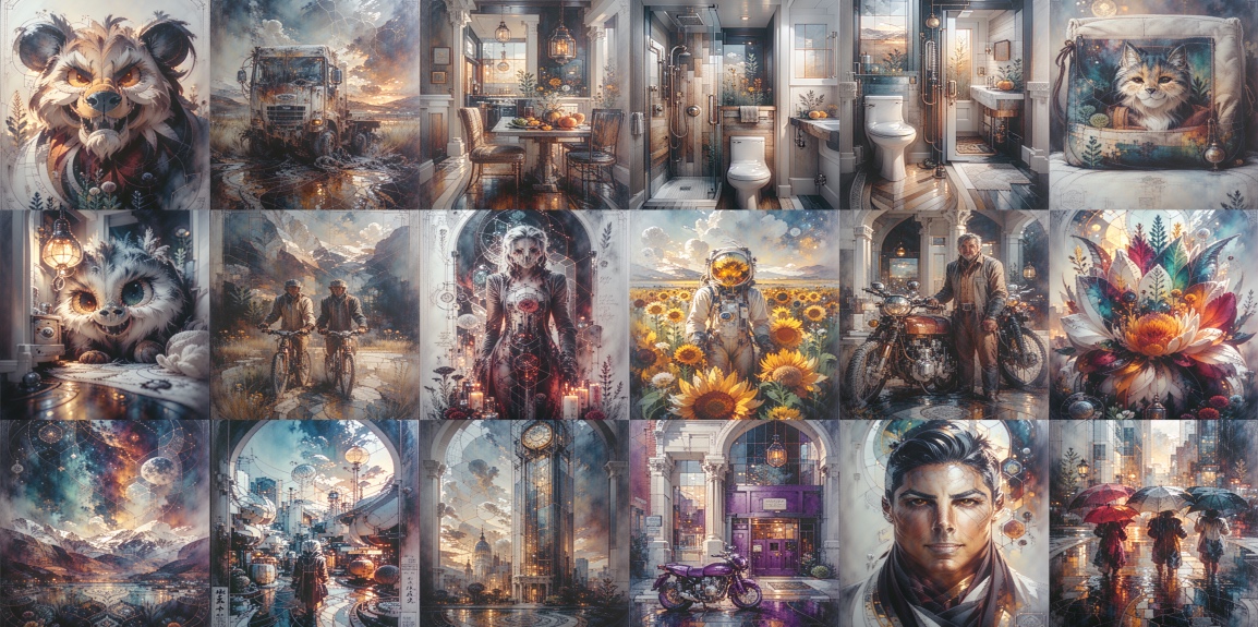
Here, we show uncurated samples from models fine-tuned with DRaFT for different reward functions: Human Preference Score v2 (Figure 33), PickScore (Figure 34), and a combined reward (Figure 35). The first two are overfit to the reward functions, which decreases diversity and photorealism. In the third, we mitigate overfitting through LoRA scaling.

Figure 33: Uncurated samples from Stable Diffusion fine-tuned using DRaFT-1 for the HPSv2 reward (Wu et al., 2023a).

Figure 34: Uncurated samples from Stable Diffusion fine-tuned using DRaFT-1 for the PickScore reward (Kirstain et al., 2023).

Figure 35: Uncurated samples from pre-trained Stable Diffusion 1.4 compared with Stable Diffusion after reward fine-tuning. We use DRaFT-LV on a combined reward of $\text{PickScore}=10,\text{HPSv2}=2,\text{Aesthetic}=0.05$. After training, LoRA weights are scaled down by a factor of 0.75 to reduce reward overfitting. Prompts are from the HPSv2 benchmark.

References

- Akrour et al. (2011) Riad Akrour, Marc Schoenauer, and Michele Sebag. Preference-based policy learning. In Machine Learning and Knowledge Discovery in Databases: European Conference, pp. 12–27, 2011.
- Askell et al. (2021) Amanda Askell, Yuntao Bai, Anna Chen, Dawn Drain, Deep Ganguli, Tom Henighan, Andy Jones, Nicholas Joseph, Ben Mann, Nova DasSarma, et al. A general language assistant as a laboratory for alignment. arXiv preprint arXiv:2112.00861, 2021.
- Bai et al. (2022a) Yuntao Bai, Andy Jones, Kamal Ndousse, Amanda Askell, Anna Chen, Nova DasSarma, Dawn Drain, Stanislav Fort, Deep Ganguli, Tom Henighan, et al. Training a helpful and harmless assistant with reinforcement learning from human feedback. arXiv preprint arXiv:2204.05862, 2022a.
- Bai et al. (2022b) Yuntao Bai, Saurav Kadavath, Sandipan Kundu, Amanda Askell, Jackson Kernion, Andy Jones, Anna Chen, Anna Goldie, Azalia Mirhoseini, Cameron McKinnon, et al. Constitutional AI: Harmlessness from AI feedback. arXiv preprint arXiv:2212.08073, 2022b.
- Bansal et al. (2023) Arpit Bansal, Hong-Min Chu, Avi Schwarzschild, Soumyadip Sengupta, Micah Goldblum, Jonas Geiping, and Tom Goldstein. Universal guidance for diffusion models. In Conference on Computer Vision and Pattern Recognition, pp. 843–852, 2023.
- Beaumont et al. (2022) Romain Beaumont, Ross Wightman, Phil Wang, Boris Dayma, Mitchell Wortsman, Blinkdl, Cristoph Schuhmann, Jenia Jitsev, Schmidt Ludwig, Mehdi Cherti, and Emad Mostaque. Large scale OpenCLIP: L/14, H/14 and G/14 trained on LAION-2B. laion.ai, 2022.
- Black et al. (2023) Kevin Black, Michael Janner, Yilun Du, Ilya Kostrikov, and Sergey Levine. Training diffusion models with reinforcement learning. arXiv preprint arXiv:2305.13301, 2023.
- Bradbury et al. (2018) James Bradbury, Roy Frostig, Peter Hawkins, Matthew James Johnson, Chris Leary, Dougal Maclaurin, George Necula, Adam Paszke, Jake VanderPlas, Skye Wanderman-Milne, and Qiao Zhang. JAX: composable transformations of Python+NumPy programs, 2018. URL http://github.com/google/jax.
- Chen et al. (2016) Tianqi Chen, Bing Xu, Chiyuan Zhang, and Carlos Guestrin. Training deep nets with sublinear memory cost. arXiv preprint arXiv:1604.06174, 2016.
- Chen et al. (2023) Xi Chen, Xiao Wang, Soravit Changpinyo, AJ Piergiovanni, Piotr Padlewski, Daniel Salz, Sebastian Goodman, Adam Grycner, Basil Mustafa, Lucas Beyer, et al. PaLi: A jointly-scaled multilingual language-image model. In International Conference on Learning Representations, 2023.
- Chen et al. (2015) Xinlei Chen, Hao Fang, Tsung-Yi Lin, Ramakrishna Vedantam, Saurabh Gupta, Piotr Dollár, and C Lawrence Zitnick. Microsoft COCO captions: Data collection and evaluation server. arXiv preprint arXiv:1504.00325, 2015.
- Christiano et al. (2017) Paul F Christiano, Jan Leike, Tom Brown, Miljan Martic, Shane Legg, and Dario Amodei. Deep reinforcement learning from human preferences. Advances in Neural Information Processing Systems, 30, 2017.
- Dhariwal & Nichol (2021) Prafulla Dhariwal and Alexander Nichol. Diffusion models beat GANs on image synthesis. Advances in Neural Information Processing Systems, 34:8780–8794, 2021.
- Dong et al. (2023) Hanze Dong, Wei Xiong, Deepanshu Goyal, Rui Pan, Shizhe Diao, Jipeng Zhang, Kashun Shum, and Tong Zhang. RAFT: Reward ranked finetuning for generative foundation model alignment. arXiv preprint arXiv:2304.06767, 2023.
- Fan et al. (2023) Ying Fan, Olivia Watkins, Yuqing Du, Hao Liu, Moonkyung Ryu, Craig Boutilier, Pieter Abbeel, Mohammad Ghavamzadeh, Kangwook Lee, and Kimin Lee. DPOK: Reinforcement learning for fine-tuning text-to-image diffusion models. arXiv preprint arXiv:2305.16381, 2023.
- Geirhos et al. (2019) Robert Geirhos, Patricia Rubisch, Claudio Michaelis, Matthias Bethge, Felix A Wichmann, and Wieland Brendel. ImageNet-trained CNNs are biased towards texture; increasing shape bias improves accuracy and robustness. In International Conference on Learning Representations, 2019.
- Glaese et al. (2022) Amelia Glaese, Nat McAleese, Maja Trębacz, John Aslanides, Vlad Firoiu, Timo Ewalds, Maribeth Rauh, Laura Weidinger, Martin Chadwick, Phoebe Thacker, et al. Improving alignment of dialogue agents via targeted human judgements. arXiv preprint arXiv:2209.14375, 2022.
- Gruslys et al. (2016) Audrunas Gruslys, Rémi Munos, Ivo Danihelka, Marc Lanctot, and Alex Graves. Memory-efficient backpropagation through time. Advances in Neural Information Processing Systems, 29, 2016.
- Gu et al. (2023) Jiatao Gu, Alex Trevithick, Kai-En Lin, Joshua M Susskind, Christian Theobalt, Lingjie Liu, and Ravi Ramamoorthi. NerfDiff: Single-image view synthesis with NeRF-guided distillation from 3d-aware diffusion. In International Conference on Machine Learning, pp. 11808–11826, 2023.
- Hao et al. (2022) Yaru Hao, Zewen Chi, Li Dong, and Furu Wei. Optimizing prompts for text-to-image generation. arXiv preprint arXiv:2212.09611, 2022.
- Ho & Salimans (2021) Jonathan Ho and Tim Salimans. Classifier-free diffusion guidance. NeurIPS Workshop on Deep Generative Models and Downstream Applications, 2021.
- Ho et al. (2020) Jonathan Ho, Ajay Jain, and Pieter Abbeel. Denoising diffusion probabilistic models. Advances in Neural Information Processing Systems, 33:6840–6851, 2020.
- Ho et al. (2022) Jonathan Ho, William Chan, Chitwan Saharia, Jay Whang, Ruiqi Gao, Alexey Gritsenko, Diederik P Kingma, Ben Poole, Mohammad Norouzi, David J Fleet, et al. Imagen video: High definition video generation with diffusion models. arXiv preprint arXiv:2210.02303, 2022.
- Hu et al. (2022) Edward J Hu, Yelong Shen, Phillip Wallis, Zeyuan Allen-Zhu, Yuanzhi Li, Shean Wang, Lu Wang, and Weizhu Chen. LoRA: Low-rank adaptation of large language models. In International Conference on Learning Representations, 2022.
- Huang et al. (2023) Chengsong Huang, Qian Liu, Bill Yuchen Lin, Tianyu Pang, Chao Du, and Min Lin. LoraHub: Efficient cross-task generalization via dynamic LoRA composition. arXiv preprint arXiv:2307.13269, 2023.
- Ibarz et al. (2018) Borja Ibarz, Jan Leike, Tobias Pohlen, Geoffrey Irving, Shane Legg, and Dario Amodei. Reward learning from human preferences and demonstrations in Atari. Advances in Neural Information Processing Systems, 31, 2018.
- Kingma et al. (2021) Diederik Kingma, Tim Salimans, Ben Poole, and Jonathan Ho. Variational diffusion models. Advances in Neural Information Processing Systems, 34:21696–21707, 2021.
- Kirstain et al. (2023) Yuval Kirstain, Adam Polyak, Uriel Singer, Shahbuland Matiana, Joe Penna, and Omer Levy. Pick-a-pic: An open dataset of user preferences for text-to-image generation. arXiv preprint arXiv:2305.01569, 2023.
- Knox & Stone (2009) W Bradley Knox and Peter Stone. Interactively shaping agents via human reinforcement: The tamer framework. In Proceedings of the fifth international Conference on Knowledge capture, pp. 9–16, 2009.
- Lee et al. (2023) Kimin Lee, Hao Liu, Moonkyung Ryu, Olivia Watkins, Yuqing Du, Craig Boutilier, Pieter Abbeel, Mohammad Ghavamzadeh, and Shixiang Shane Gu. Aligning text-to-image models using human feedback. arXiv preprint arXiv:2302.12192, 2023.
- Li et al. (2022) Wei Li, Xue Xu, Xinyan Xiao, Jiachen Liu, Hu Yang, Guohao Li, Zhanpeng Wang, Zhifan Feng, Qiaoqiao She, Yajuan Lyu, et al. UPainting: Unified text-to-image diffusion generation with cross-modal guidance. arXiv preprint arXiv:2210.16031, 2022.
- Lillicrap et al. (2016) Timothy P Lillicrap, Jonathan J Hunt, Alexander Pritzel, Nicolas Heess, Tom Erez, Yuval Tassa, David Silver, and Daan Wierstra. Continuous control with deep reinforcement learning. In International Conference on Learning Representations, 2016.
- Liu et al. (2023) Haohe Liu, Zehua Chen, Yi Yuan, Xinhao Mei, Xubo Liu, Danilo Mandic, Wenwu Wang, and Mark D Plumbley. AudioLDM: Text-to-audio generation with latent diffusion models. In Proceedings of Machine Learning Research, 2023.
- Liu et al. (2022) Nan Liu, Shuang Li, Yilun Du, Antonio Torralba, and Joshua B Tenenbaum. Compositional visual generation with composable diffusion models. In European Conference on Computer Vision, pp. 423–439, 2022.
- Loshchilov & Hutter (2019) Ilya Loshchilov and Frank Hutter. Decoupled weight decay regularization. In International Conference on Learning Representations, 2019.
- Meng et al. (2023) Chenlin Meng, Robin Rombach, Ruiqi Gao, Diederik Kingma, Stefano Ermon, Jonathan Ho, and Tim Salimans. On distillation of guided diffusion models. In Conference on Computer Vision and Pattern Recognition, pp. 14297–14306, 2023.
- Minderer et al. (2022) Matthias Minderer, Alexey Gritsenko, Austin Stone, Maxim Neumann, Dirk Weissenborn, Alexey Dosovitskiy, Aravindh Mahendran, Anurag Arnab, Mostafa Dehghani, Zhuoran Shen, et al. Simple open-vocabulary object detection. In European Conference on Computer Vision, pp. 728–755, 2022.
- Nichol et al. (2021) Alex Nichol, Prafulla Dhariwal, Aditya Ramesh, Pranav Shyam, Pamela Mishkin, Bob McGrew, Ilya Sutskever, and Mark Chen. Glide: Towards photorealistic image generation and editing with text-guided diffusion models. arXiv preprint arXiv:2112.10741, 2021.
- Ouyang et al. (2022) Long Ouyang, Jeffrey Wu, Xu Jiang, Diogo Almeida, Carroll Wainwright, Pamela Mishkin, Chong Zhang, Sandhini Agarwal, Katarina Slama, Alex Ray, et al. Training language models to follow instructions with human feedback. Advances in Neural Information Processing Systems, 35:27730–27744, 2022.
- Paszke et al. (2019) Adam Paszke, Sam Gross, Francisco Massa, Adam Lerer, James Bradbury, Gregory Chanan, Trevor Killeen, Zeming Lin, Natalia Gimelshein, Luca Antiga, et al. Pytorch: An imperative style, high-performance deep learning library. Advances in Neural Information Processing Systems, 32, 2019.
- Poole et al. (2023) Ben Poole, Ajay Jain, Jonathan T Barron, and Ben Mildenhall. Dreamfusion: Text-to-3d using 2d diffusion. In International Conference on Learning Representations, 2023.
- Radford et al. (2021) Alec Radford, Jong Wook Kim, Chris Hallacy, Aditya Ramesh, Gabriel Goh, Sandhini Agarwal, Girish Sastry, Amanda Askell, Pamela Mishkin, Jack Clark, et al. Learning transferable visual models from natural language supervision. In International Conference on Machine Learning, pp. 8748–8763, 2021.
- Ramesh et al. (2021) Aditya Ramesh, Mikhail Pavlov, Gabriel Goh, Scott Gray, Chelsea Voss, Alec Radford, Mark Chen, and Ilya Sutskever. Zero-shot text-to-image generation. In International Conference on Machine Learning, pp. 8821–8831, 2021.
- Ramesh et al. (2022) Aditya Ramesh, Prafulla Dhariwal, Alex Nichol, Casey Chu, and Mark Chen. Hierarchical text-conditional image generation with CLIP latents. arXiv preprint arXiv:2204.06125, 2022.
- Rombach et al. (2022) Robin Rombach, Andreas Blattmann, Dominik Lorenz, Patrick Esser, and Björn Ommer. High-resolution image synthesis with latent diffusion models. In Proceedings of the IEEE/CVF Conference on Computer Vision and Pattern Recognition, pp. 10684–10695, 2022.
- Ronneberger et al. (2015) Olaf Ronneberger, Philipp Fischer, and Thomas Brox. U-Net: Convolutional networks for biomedical image segmentation. In Medical Image Computing and Computer-Assisted Intervention International Conference, pp. 234–241, 2015.
- Saharia et al. (2022) Chitwan Saharia, William Chan, Saurabh Saxena, Lala Li, Jay Whang, Emily Denton, Seyed Kamyar Seyed Ghasemipour, Burcu Karagol Ayan, S Sara Mahdavi, Rapha Gontijo Lopes, et al. Photorealistic text-to-image diffusion models with deep language understanding. Advances in Neural Information Processing Systems, 2022.
- Schuhmann & Beaumont (2022) Christoph Schuhmann and Romain Beaumont. LAION-aesthetics. laion.ai, 2022.
- Silver et al. (2014) David Silver, Guy Lever, Nicolas Heess, Thomas Degris, Daan Wierstra, and Martin Riedmiller. Deterministic policy gradient algorithms. In International Conference on Machine Learning, pp. 387–395, 2014.
- Singer et al. (2023) Uriel Singer, Adam Polyak, Thomas Hayes, Xi Yin, Jie An, Songyang Zhang, Qiyuan Hu, Harry Yang, Oron Ashual, Oran Gafni, et al. Make-a-video: Text-to-video generation without text-video data. In International Conference on Learning Representations, 2023.
- Sohl-Dickstein et al. (2015) Jascha Sohl-Dickstein, Eric Weiss, Niru Maheswaranathan, and Surya Ganguli. Deep unsupervised learning using nonequilibrium thermodynamics. In International Conference on Machine Learning, pp. 2256–2265, 2015.
- Song et al. (2021a) Jiaming Song, Chenlin Meng, and Stefano Ermon. Denoising diffusion implicit models. In International Conference on Learning Representations, 2021a.
- Song & Ermon (2019) Yang Song and Stefano Ermon. Generative modeling by estimating gradients of the data distribution. Advances in Neural Information Processing Systems, 32, 2019.
- Song et al. (2021b) Yang Song, Jascha Sohl-Dickstein, Diederik P Kingma, Abhishek Kumar, Stefano Ermon, and Ben Poole. Score-based generative modeling through stochastic differential equations. In International Conference on Learning Representations, 2021b.
- Stiennon et al. (2020) Nisan Stiennon, Long Ouyang, Jeffrey Wu, Daniel Ziegler, Ryan Lowe, Chelsea Voss, Alec Radford, Dario Amodei, and Paul F Christiano. Learning to summarize with human feedback. Advances in Neural Information Processing Systems, 33:3008–3021, 2020.
- Wallace et al. (2023) Bram Wallace, Akash Gokul, Stefano Ermon, and Nikhil Naik. End-to-end diffusion latent optimization improves classifier guidance. arXiv preprint arXiv:2303.13703, 2023.
- Wang et al. (2023) Zijie J Wang, Evan Montoya, David Munechika, Haoyang Yang, Benjamin Hoover, and Duen Horng Chau. Diffusiondb: A large-scale prompt gallery dataset for text-to-image generative models. In Association for Computational Linguistics, 2023.
- Watson et al. (2021) Daniel Watson, William Chan, Jonathan Ho, and Mohammad Norouzi. Learning fast samplers for diffusion models by differentiating through sample quality. In International Conference on Learning Representations, 2021.
- Williams (1992) Ronald J Williams. Simple statistical gradient-following algorithms for connectionist reinforcement learning. Machine Learning, 8:229–256, 1992.
- Wortsman et al. (2022) Mitchell Wortsman, Gabriel Ilharco, Samir Ya Gadre, Rebecca Roelofs, Raphael Gontijo-Lopes, Ari S Morcos, Hongseok Namkoong, Ali Farhadi, Yair Carmon, Simon Kornblith, et al. Model soups: averaging weights of multiple fine-tuned models improves accuracy without increasing inference time. In International Conference on Machine Learning, pp. 23965–23998, 2022.
- Wu et al. (2021) Jeff Wu, Long Ouyang, Daniel M Ziegler, Nisan Stiennon, Ryan Lowe, Jan Leike, and Paul Christiano. Recursively summarizing books with human feedback. arXiv preprint arXiv:2109.10862, 2021.
- Wu et al. (2023a) Xiaoshi Wu, Yiming Hao, Keqiang Sun, Yixiong Chen, Feng Zhu, Rui Zhao, and Hongsheng Li. Human preference score v2: A solid benchmark for evaluating human preferences of text-to-image synthesis. arXiv preprint arXiv:2306.09341, 2023a.
- Wu et al. (2023b) Xiaoshi Wu, Keqiang Sun, Feng Zhu, Rui Zhao, and Hongsheng Li. Better aligning text-to-image models with human preference. arXiv preprint arXiv:2303.14420, 2023b.
- Xu et al. (2023) Jiazheng Xu, Xiao Liu, Yuchen Wu, Yuxuan Tong, Qinkai Li, Ming Ding, Jie Tang, and Yuxiao Dong. Imagereward: Learning and evaluating human preferences for text-to-image generation. arXiv preprint arXiv:2304.05977, 2023.
- Zeng et al. (2022) Xiaohui Zeng, Arash Vahdat, Francis Williams, Zan Gojcic, Or Litany, Sanja Fidler, and Karsten Kreis. LION: Latent point diffusion models for 3d shape generation. In Advances in Neural Information Processing Systems (NeurIPS), 2022.
- Zhang et al. (2023) Jinghan Zhang, Shiqi Chen, Junteng Liu, and Junxian He. Composing parameter-efficient modules with arithmetic operations. arXiv preprint arXiv:2306.14870, 2023.
- Zhang et al. (2018) Richard Zhang, Phillip Isola, Alexei A Efros, Eli Shechtman, and Oliver Wang. The unreasonable effectiveness of deep features as a perceptual metric. In Conference on Computer Vision and Pattern Recognition, 2018.
- Ziegler et al. (2019) Daniel M Ziegler, Nisan Stiennon, Jeffrey Wu, Tom B Brown, Alec Radford, Dario Amodei, Paul Christiano, and Geoffrey Irving. Fine-tuning language models from human preferences. arXiv preprint arXiv:1909.08593, 2019.