Singular value decomposition quantum algorithm for quantum biology

Abstract

There has been a recent interest in quantum algorithms for the modelling and prediction of non-unitary quantum dynamics using current quantum computers. The field of quantum biology is one area where these algorithms could prove to be useful, as biological systems are generally intractable to treat in their complete form, but amenable to an open quantum systems approach. Here we present the application of a recently developed singular value decomposition algorithm to two well-studied benchmark systems in quantum biology: excitonic energy transport through the Fenna-Matthews-Olson complex and the radical pair mechanism for avian navigation. We demonstrate that the singular value decomposition algorithm is capable of capturing accurate short- and long-time dynamics for these systems through implementation on a quantum simulator, and conclude that this algorithm has the potential to be an effective tool for the future study of systems relevant to quantum biology.

I Introduction

There are very few systems which exist in a vacuum; the majority of real physical systems interact with their environments in a non-trivial way. This is especially true for systems of biological relevance, where there is often a large and complex environment surrounding any energy or information transport process. Modelling these processes exactly is frequently computationally intractable; however, they are amenable to an open quantum system treatment [1]. Standard methods in open quantum systems, such as the Lindblad equation [2, 3, 4], are capable of accurately describing a variety of biologically relevant dynamical processes, including excitonic energy transport in photosynthetic light-harvesting antennae [1, 5, 6, 7, 8, 9, 10], radical pair mechanisms for avian navigation [11, 12, 13] and other physiological functions [14], and transport through ion channels [15, 16, 17, 18].

An important aspect of recent quantum algorithm development has focused on the modelling of open quantum systems [19], which are systems that are not isolated but instead interact with their surroundings and are generally characterized by non-unitary dynamics. The challenge in developing gate-based quantum algorithms to capture these dynamical processes is that only unitary gates can be implemented on current quantum computers, but open quantum systems exhibit non-unitary time dynamics. A variety of algorithms have been developed to overcome this obstacle [20, 21, 22], often using block encoding techniques [23, 24, 25, 26, 27, 28, 29]. Recently, two of the authors used classical computation of the singular value decomposition (SVD) of the time propagating operator, followed by an implementation of the dynamics with the singular value matrix on a quantum device. While this algorithm requires a non-negligible classical cost, the non-unitary component is mapped entirely to the diagonal singular-value matrix, and this sparsity can be leveraged when encoding the dynamics in a quantum circuit. The SVD has effectively been used to consider open quantum system evolution and general non-normalized state preparation [27]. Here, we will use this algorithm to simulate the non-unitary dynamics of two systems in quantum biology: excitonic energy transport through a photosynthetic light-harvesting antenna, and the radical pair mechanism for avian navigation.

First, we will consider the Fenna-Matthews-Olson (FMO) complex, which is a well-studied biological complex vital to photosynthetic light harvesting in green sulfur bacteria [30]. It exists as a trimer in the bacteria between the light-harvesting antenna and photosynthetic reaction center where it facilitates efficient exciton transfer. This is shown schematically in Figure 1, where an exciton is transferred into the complex on site 1, transported among the other sites, and eventually passes from site 3 to the reaction center where it can be converted into usable energy for the bacterium. While there have been extensive theoretical and experimental studies on this complex [31, 32, 33, 34, 35, 36], few have utilized quantum algorithms, and the long-time dynamics have remained challenging to simulate [26].

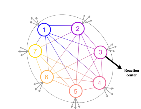
Figure 1: Schematic depiction of one trimer of the Fenna-Matthews-Olson complex, showing sites 1-7. The colors represent Hamiltonian terms, both on-site and between-site couplings. The grey arrows represent dissipation and decoherence due to the environment, and the black arrow represents the coupling of site 3 to the reaction center.

The second system that we will study is the radical pair mechanism (RPM) proposed for avian navigation [11]. The RPM is theorized to explain how migratory birds can sense and navigate along Earth’s magnetic field [37, 38, 39, 40, 41]. The basic scheme is represented in Figure 2. First, a donor molecule is excited by incoming light, causing the transfer of an electron from the donor to an acceptor molecule, creating a pair of coupled radicals. The radical pair is initially in the singlet state, but can interconvert between three triplet states as well. This conversion is partly determined by a coupled nuclear spin and the direction and strength of an external magnetic field. Depending on the spin state of the pair when they recombine, different chemical signals result. The yields of singlet and triplet products can therefore signal information about the orientation of the electron spin with respect to the external field. This particular application has also been extensively investigated theoretically [11, 37, 40, 41, 12, 13, 42], including a quantum algorithm investigation [43], making it a good benchmark for the ability of a quantum algorithm to effectively capture a radical pair mechanism, which is prevalent in many other physiological processes [14].

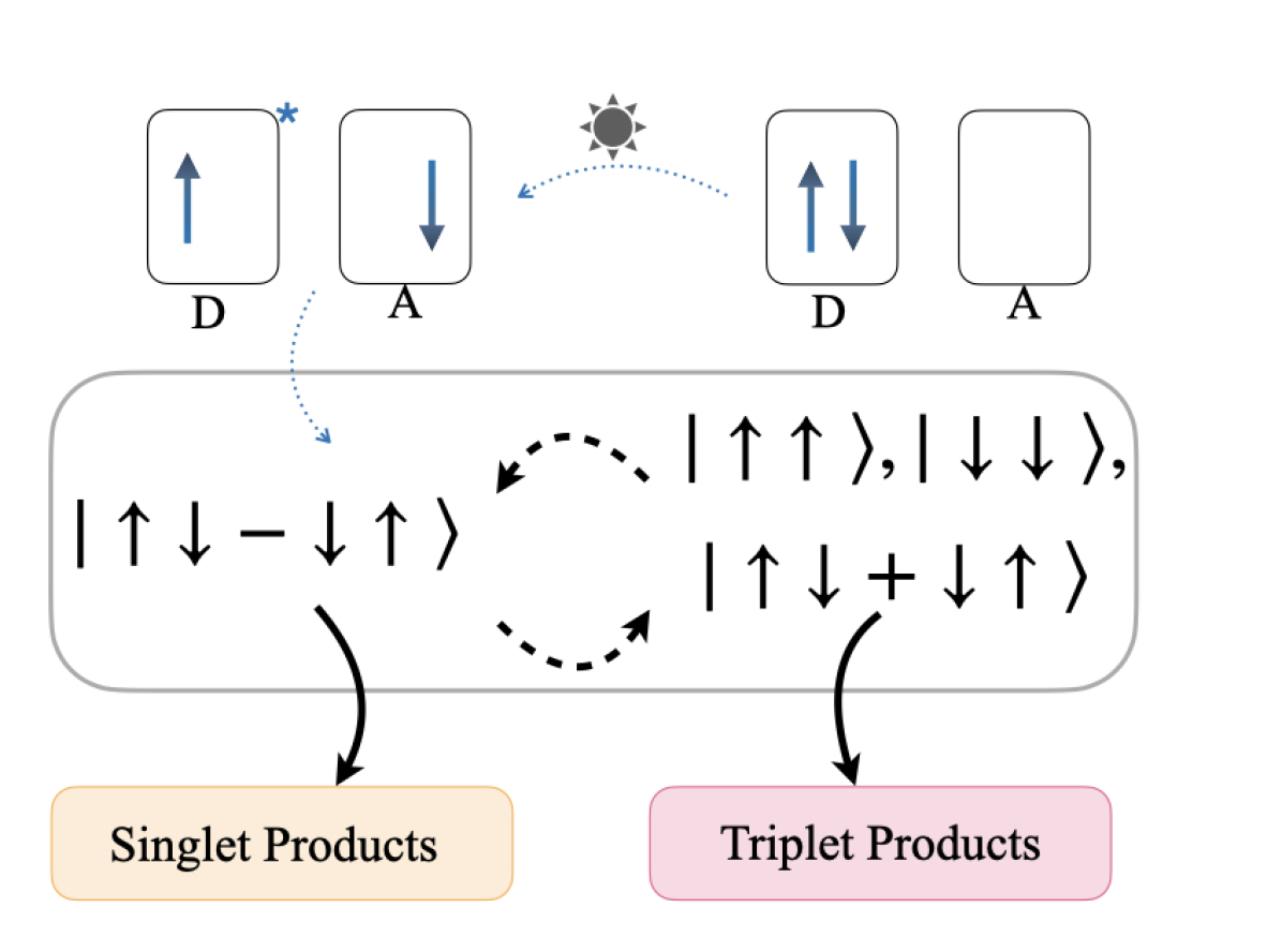
Figure 2: The radical pair mechanism: Excitation of the donor molecule, D, and the transfer of the electron to the acceptor, A, is shown along with the interconversion between singlet and triplet states and recombination. One of the electrons is coupled to a nuclear spin not shown in the above schematic.

In Section II we will review both the open quantum systems framework and the singular value decomposition algorithm. We will then present results using this algorithm for two systems, outlined above, in Section III. Finally, we will discuss these results in the context of the potential for quantum algorithms to model and predict quantum systems of biological relevance in Section IV.

II Methods

II.1 Lindblad approach to dissipative quantum systems

A common model for the description of Markovian open quantum system dynamics is the Gorini–Kossakowski–Sudarshan–Lindblad (GKSL) master equation [2, 3, 4],

$$\frac{d\rho}{dt}=-i[\hat{H},\rho]+\sum_{i}\gamma_{i}\big{(}\hat{C}_{i}\rho\hat{C}_{i}^{\dagger}-\frac{1}{2}\{\hat{C}_{i}^{\dagger}\hat{C}_{i},\rho\}\big{)},$$ (1)

where $\hat{H}$ is the system Hamiltonian, $\rho$ is the density matrix, and $\gamma_{i}$ are the decay rates corresponding to the physically relevant Lindbladian operators, $\hat{C}_{i}$.

For the models constructed for this paper, the unravelled master equation form was used [44, 28]. In this form the superoperator can be written as:

$$\hat{\mathcal{L}} =-i\mathbb{I}\otimes\hat{H}+i\hat{H}^{T}\otimes\mathbb{I}$$ (2)

$$+\sum_{i}\gamma_{i}(\hat{C}_{i}^{*}\otimes\hat{C}_{i}-\frac{1}{2}\mathbb{I}\otimes\hat{C}_{i}^{\dagger}\hat{C}_{i}-\frac{1}{2}\hat{C}_{i}^{T}\hat{C}_{i}^{*}\otimes\mathbb{I})$$

such that the time evolved vectorized density matrix can be determined as,

$$\ket{\rho(t)}=e^{\hat{\mathcal{L}}t}\ket{\rho(0)}.$$ (3)

We note that $\mathbb{I}$ is the identity matrix and $*$, $\dagger$, and $T$ are the complex conjugate, adjoint, and transpose operations, respectively.

II.2 Singular value decomposition based non-unitary quantum dynamics

The Lindblad equation models non-unitary evolution, so the propagator $\hat{M}=e^{\hat{\mathcal{L}}t}$ needs to be mapped into a unitary form that can be implemented on current quantum devices. We begin with the SVD written as,

$$\hat{M}=\hat{U}\hat{\Sigma}\hat{V}^{\dagger}$$ (4)

where $\hat{U}$ and $\hat{V}^{\dagger}$ are unitary operators, and $\hat{\Sigma}$ is a real non-unitary diagonal operator. The diagonal operator can be dilated into a unitary (and diagonal) operator,

$$\hat{U}_{\hat{\Sigma}}=\begin{pmatrix}\hat{\Sigma}_{+}&0\\ 0&\hat{\Sigma}_{-}\end{pmatrix},$$ (5)

in which

$$\hat{\Sigma}_{i,\pm}=\sigma_{i}\pm i\sqrt{\frac{1-\sigma_{i}^{2}}{\sigma_{i}^{2}}}\sigma_{i},$$ (6)

where $\sigma_{i}$ are the singular values of $\hat{M}$.

Therefore, the non-unitary operator $\hat{M}$ can be implemented on a quantum circuit as seen in Figure 3, where $k$ denotes that the system wavefunction spans multiple qubits. This approach is not deterministic, and the state $M(t)\lvert 0\rangle=\lvert\psi(t)\rangle$ is prepared only when the ancilla qubit is measured in state $\lvert 0\rangle$.

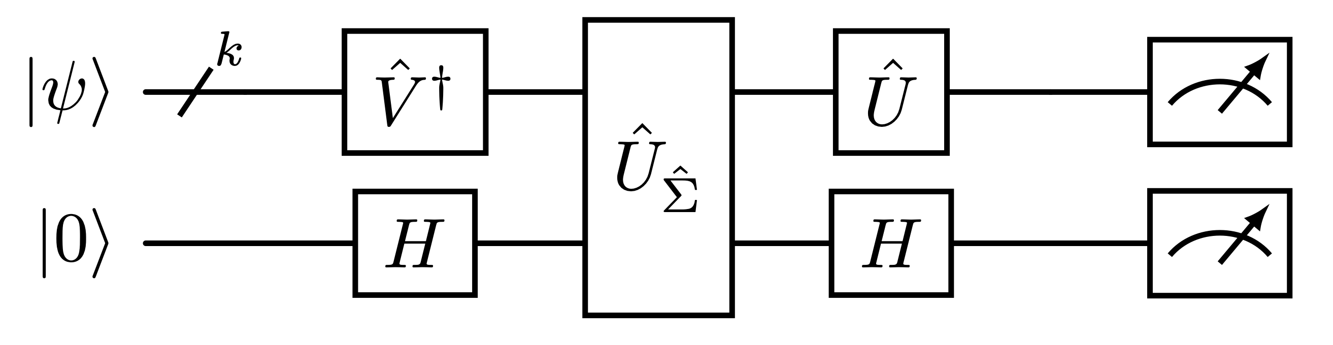
Figure 3: Quantum circuit for a non-unitary operator acting on a state, $\ket{\psi}$, by using the singular value decomposition and dilating the diagonal operator. The system spans $k$ qubits and the single additional ancilla bit is initialized in the ground state, $\ket{0}$.

If a unitary matrix is size $r$, then it can be mapped to $k$-qubit unitary gates where $k\geq\log_{2}(r)$. The dilation of a non-unitary matrix adds an additional qubit resulting in $d=k+1$ qubits required to simulate the SVD of the non-unitary operator. The dilated singular value matrix can be implemented exactly with $\mathcal{O}(2^{d+1})$ gates, although polynomially scaling approximations are also available [45]. The unitaries $\hat{U}$ and $\hat{V}^{\dagger}$ each require $\mathcal{O}((d-1)^{2}2^{2d-2})$ gates. The total gate complexity of the SVD algorithm is therefore $\mathcal{O}(d^{2}2^{2d-1})$ [27]. In the limit of large system size, the application of $\hat{U}$ and $\hat{V}^{\dagger}$ to the quantum register generates the most overhead. In the asymptotic limit, given access to the SVD, a $d$-qubit non-unitary operator can be applied to a quantum register for approximately twice the cost of a $d$-qubit unitary operator.

Beyond the gate complexity of the circuit, there are other cost factors to consider. First, the singular value decomposition is computed classically with a complexity $\mathcal{O}(r^{3})$ where $r$ is the size of the decomposed operator. When computed numerically, the SVD scaling is prohibitive for arbitrarily large or complex matrices; however, operators used in the context of Noisy-Intermediate-Scale Quantum (NISQ) devices are modestly sized and the SVD is easily computed classically. In addition, physical processes may have SVDs which can be written analytically [27], and there are also quantum algorithms for computing the SVD in the fault-tolerant regime [29, 46]. Secondly, to obtain accurate long-time dynamics, the unravelled or vectorized master equation must be used. This involves transitioning from a Hilbert space of size $r$ to the Liouville space of size $r^{2}$ which also spans a larger qubit space. This mapping requires a larger number of qubits and therefore an increase in complexity; however, it allows for simulating long-time dynamics without approximating the solution to the differential Lindblad equation.

III Results

III.1 Light-harvesting antennae

The exciton dynamics in the FMO complex have been successfully modelled classically by the Lindblad equation [1, 5, 6, 7, 8, 9, 10, 26], where the coherent or unitary components are described by the Hamiltonian,

$$\hat{H}_{FMO}=\sum_{i=1}^{7}\omega_{i}\sigma_{i}^{+}\sigma_{i}^{-}+\sum_{j\neq i}J_{ij}(\sigma_{i}^{+}\sigma_{j}^{-}+\sigma_{j}^{+}\sigma_{i}^{-}),$$ (7)

where $\sigma_{i}^{+}$ and $\sigma_{i}^{-}$ are the creation and annihilation operators respectively, $\omega_{i}$ is the on-site coupling, and $J_{ij}$ is the coupling between sites $i$ and $j$. We use the coupling parameters from Ref. 1, and the full Hamiltonian in matrix form can be found in the Supplementary Information.

In the schematic of the full system in Figure 1, the Hamiltonian terms accounting for the on-site chromophore energies are depicted by circled numbers and their couplings by lines. The Lindbladian terms account for the transfer of the exciton from the third chromophore to the sink, which models the reaction center, as well as dephasing and dissipation to the ground state. Transfer to the sink is represented by black arrows, and dephasing and dissipation by grey arrows in the schematic. These Lindbladians take the form,

$$\hat{C}_{deph}(i)=\sqrt{\gamma_{deph}}\ket{i}\bra{i}$$ (8)

$$\hat{C}_{diss}(i)=\sqrt{\gamma_{diss}}\ket{0}\bra{i}$$

$$\hat{C}_{sink}=\sqrt{\gamma_{sink}}\ket{8}\bra{3},$$

where $i$ is an integer on the range $[1,7]$, states $\ket{0}$ and $\ket{8}$ model the ground and sink sites, respectively, and $\gamma_{deph}$, $\gamma_{diss}$, and $\gamma_{sink}$ represent the corresponding rates of dephasing, dissipation, and transfer to the sink for the 7-site model. Previous work has focused on the dynamics of a subsystem of this complex, [9, 26] which includes only the first 3 chromophores. For this 3-site model, $i$ is an integer only on the range $[1,3]$, and the sink is given by state $\lvert 4\rangle$ instead of $\lvert 8\rangle$. For both models, the system is initialized with the excitation on site 1.

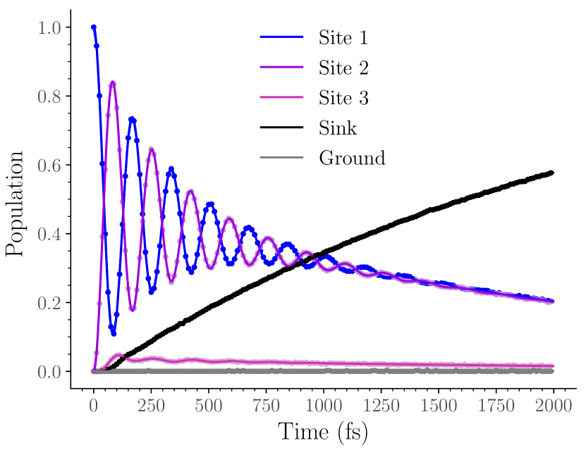
Figure 4: The time evolution of the 3 site FMO complex. The lines indicate classical results and the dots the quantum simulation. A time step of $\delta t=5$ femtoseconds (fs) and end time of 2000 fs was used. For each time point, $2^{19}$ samples were taken.

Utilizing the above parameters with the unravelled master equation in Eq. 2 and performing the singular value decomposition on the resulting operator, $\hat{M}=e^{\hat{\mathcal{L}t}}$, we can obtain results for the 3-site model. The classical baseline and quantum simulation for the dynamics can be seen in Figure 4 where the classical results are shown as solid lines and the quantum simulation as dots. A total duration of 2000 femtoseconds (fs) was used with a time step of 5 fs. For the quantum simulation results, 6 qubits were required and $2^{19}$ samples were used. These results show agreement between the quantum simulation and classical result for the entirety of the 2000 fs process, significantly extending the previous simulation time range while still maintaining accuracy [26].

We also expand the focus to the entire 7 chromophore system dynamics, which becomes a 9 level system when a sink and a ground state are included. This is demonstrated in Figure 5, where again the classical solution is shown by solid lines and the results of quantum simulation using 8 qubits and $2^{19}$ shots are shown as dots. These quantum simulation results are also in excellent agreement with the classical solution.

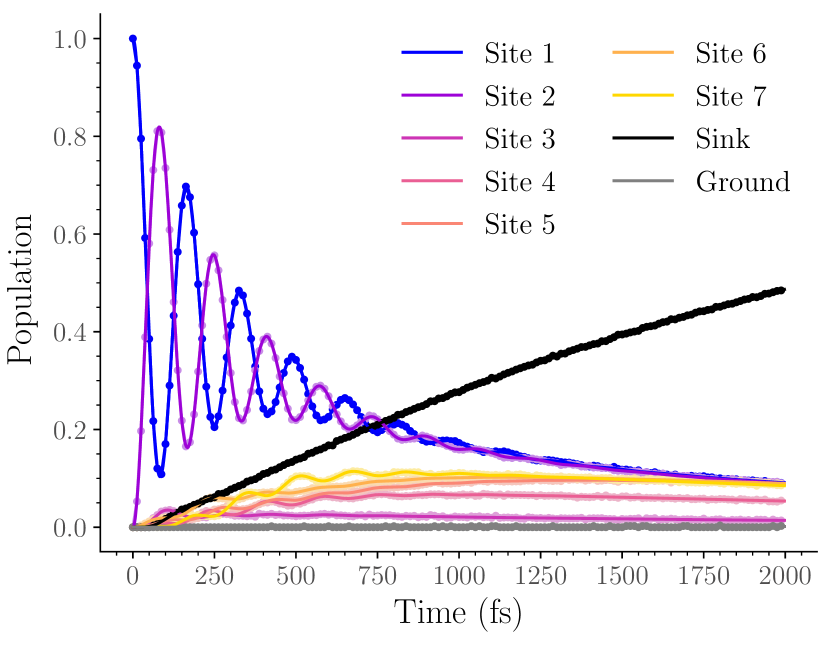
Figure 5: The classical (lines) and quantum simulation (dots) time evolution of the 7 site FMO complex. For both data sets, a time jump of $\delta t=5$ femtoseconds was used. For the quantum calculations, $2^{19}$ shots per measurement were taken.

Both the 3-site and 7-site models of excitonic dynamics in the FMO antenna demonstrate the capacity of the singular value decomposition algorithm to capture accurate dynamics on a quantum simulator, regardless of the length of time of the simulation.

III.2 Avian compass

The radical pair mechanism in the avian compass relies on the interconversion between singlet and triplet electronic states in an external magnetic field coupled to a single nuclear spin. This can be modelled with the Hamiltonian that takes the Zeeman and hyperfine interactions into account [11],

$$H=\hat{I}\cdot A\cdot\hat{S_{1}}+\gamma B\cdot(\hat{S_{1}}+\hat{S_{2}}),$$ (9)

where $\hat{I}$ is the single nuclear spin operator, $A$ is the hyperfine tensor describing the anisotropic coupling between the nucleus and the first electron, $\hat{S}_{j}$ are the electron spin operators for electrons $j=1,2$, $\gamma$ is the gyromagnetic ratio, and $B$ is the applied magnetic field given by $B=B_{0}(\cos{\phi}\sin{\theta},\sin{\phi}\sin{\theta},\cos{\theta})$. The angles $\phi$ and $\theta$ describe the radical pair’s orientation with respect to the external applied field, and based on symmetry $\phi$ can be set to zero. Due to the spatial separation of the electrons, only one electron is coupled to the nuclear spin in the Hamiltonian. The second electron is farther from, and thus much more weakly coupled to, the nuclear spin [11].

The singlet and triplet states in the electronic system can be written as,

$$\ket{s}=\frac{1}{\sqrt{2}}(\ket{\uparrow}\otimes\ket{\downarrow}-\ket{\downarrow}\otimes\ket{\uparrow})$$ (10)

$$\ket{t_{-}}=\ket{\downarrow}\otimes\ket{\downarrow}$$

$$\ket{t_{0}}=\frac{1}{\sqrt{2}}(\ket{\uparrow}\otimes\ket{\downarrow}+\ket{\downarrow}\otimes\ket{\uparrow})$$

$$\ket{t_{+}}=\ket{\uparrow}\otimes\ket{\uparrow},$$

where up and down arrows are used to represent $\alpha$ and $\beta$ spin states.

Coupling the electronic states with a single nuclear spin produces an 8 site model. Shelving states $\ket{S}$ and $\ket{T}$ are added to indicate the yields of recombination products from the given radical pair conditions. They are only connected to the system through the following Lindblad operators,

$$C_{1} =\ket{S}\bra{\uparrow,s} C_{2} =\ket{T}\bra{\uparrow,t_{0}}$$ (11)

$$C_{3} =\ket{T}\bra{\uparrow,t_{+}} C_{4} =\ket{T}\bra{\uparrow,t_{-}}$$

$$C_{5} =\ket{S}\bra{\downarrow,s} C_{6} =\ket{T}\bra{\downarrow,t_{0}}$$

$$C_{7} =\ket{T}\bra{\downarrow,t_{+}} C_{8} =\ket{T}\bra{\downarrow,t_{-}},$$

where the $s$, $t_{0}$, $t_{+}$, and $t_{-}$ indicate the spin configuration of the radical pair of electrons, and the arrows signify the direction of the nuclear spin. The decay rates for all the shelving Lindbladians are, for the sake of simplicity, made equal and given by, $\gamma_{shelf}$. Operators $C_{1}$ and $C_{5}$ show recombination from the singlet radical configuration resulting in singlet products regardless of nuclear spin. The other six operators populate the triplet yield from the three possible triplet configurations for both nuclear spins.

This model was implemented through classical Lindbladian evolution and simulated through the SVD algorithm to find the time evolution of the singlet and triplet yields. An initial pure singlet and mixed nuclear state was used. The populations obtained from setting the external magnetic field to $B_{0}=47\mu$T, the decay constant to $\gamma_{shelf}=10^{4}$, and the angle to $\theta=\frac{\pi}{2}$ can be found in Figure 6. An orientation angle of $\theta=\frac{\pi}{2}$ indicates the external field is perpendicular to the radical pair. For the quantum simulation results, 8 qubits were required and $2^{19}$ samples were used.

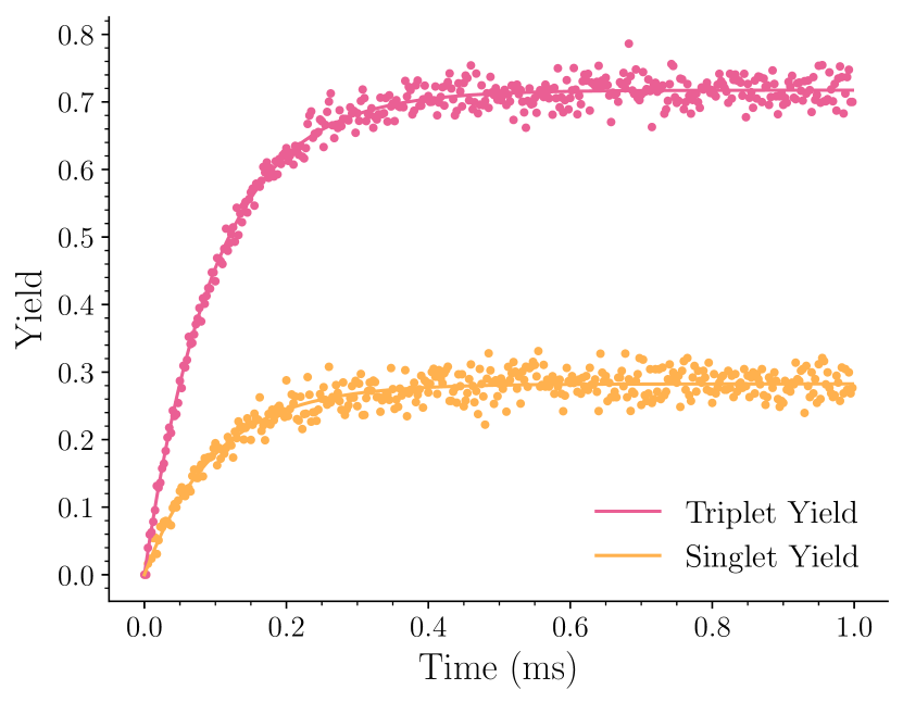
Figure 6: Singlet and triplet yields over time for the avian compass. Classical (solid) and quantum simulated (dotted) results are shown for an end time of 1 ms and a time step of $\delta t=1.75\cdot 10^{-3}$ ms. The decay constant and angle between the radical pair and external field were fixed at $\gamma_{shelf}=10^{4}$ and $\theta=\frac{\pi}{2}$, respectively.

This model so far assumes that there is no dissipation from the singlet or triplet electronic states, when in reality these states will also be dephasing while the radical pair is converting between them. This can be accounted for in the model with the addition of the following Lindbladians,

$$C_{9} =\mathbb{I}\otimes\sigma_{x}\otimes\mathbb{I} C_{10} =\mathbb{I}\otimes\mathbb{I}\otimes\sigma_{x}$$ (12)

$$C_{11} =\mathbb{I}\otimes\sigma_{y}\otimes\mathbb{I} C_{12} =\mathbb{I}\otimes\mathbb{I}\otimes\sigma_{y}$$

$$C_{13} =\mathbb{I}\otimes\sigma_{z}\otimes\mathbb{I} C_{14} =\mathbb{I}\otimes\mathbb{I}\otimes\sigma_{z},$$

where $\sigma_{i}$ are the Pauli operators and $\mathbb{I}$ is the identity matrix. The Lindbladians in Eq. 12 use the decay constant $\gamma_{diss}$ and are padded with zeros to match the dimensionality of the shelving states. Considering three different decay rates, the singlet yields compared to the orientation angle between the radical pair and external magnetic field are shown in Figure 7, where the classical solution is shown with solid lines and the quantum simulation is shown as dots. Again, 8 qubits were required and $2^{19}$ measurements were used for sampling.

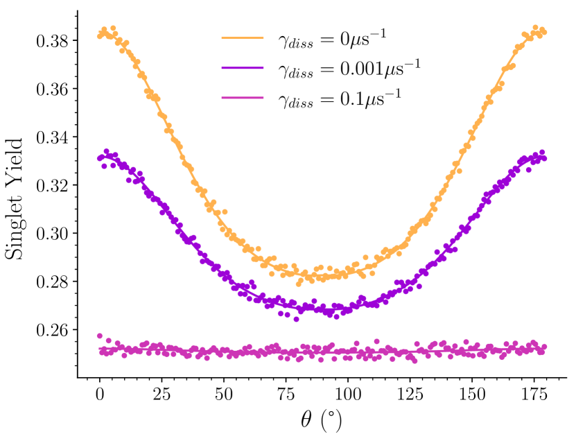
Figure 7: The angle dependence of the avian compass singlet yields with and without noise from the environment. Solid curves show exact classical SVD calculations and dots show the quantum simulation. The rate of decay to the shelving states is $\gamma_{shelf}=10^{4}$ and a theta jump of $\delta\theta=0.9^{\circ}$ was used.

The algorithm results are in good agreement with the classical solution and demonstrates that greater dissipation rates lead to less differentiation in singlet and triplet yields across a range of orientation angles. Thus, the efficacy of the avian compass is supressed with increased dissipation. For both the dissipation-free and dissipation models of the RPM, the SVD algorithm accurately captures the dynamics in all tested parameter regimes.

IV Discussion

Here we demonstrate the success of the singular value decomposition algorithm on a variety of systems pertinent to quantum biology. An important consequence of vectorization of the Lindblad dynamics is the retention of the complete (generally mixed) density matrix at each step of the dynamics. This is in contrast to the operator-sum approach where the density matrix is reconstructed from several quantum circuits. Possibly more importantly, Kraus maps are known for only a few systems, so the representation of the open quantum system dynamics is often simpler in Lindblad form. Vectorizing the Lindblad equation has a quadratic overhead in the system dimension, doubling the size of the qubit space required for the simulation. On the other hand, the vectorized form does not rely on knowledge of the Kraus maps, avoids solving the differential equation on the original Hilbert space, and allows for direct simulation of the mixed state density matrix, albeit in unravelled form.

When coupled with this superoperator representation, the SVD-based algorithm allows for simulation of long-time dynamics in a way that requires only sparse (diagonal) operations over the dilated Hilbert space, along with unitary operations on the original Hilbert space. Previous algorithms which focus on the sequential summation of Kraus maps over the time-range of the dynamics result in exponentially increasing cost as the simulation time increases. While this nesting can also be avoided using an Sz.-Nagy dilation of the superoperator, the Sz.-Nagy dilation produces an operator which acts over the entirety of the dilated Hilbert space.

The results are a step towards using quantum algorithms to predict and explore quantum phenomena in biological processes, however, it should be noted that the systems studied are beyond the scope of possible implementation on current NISQ computers. The smallest system considered here, the 3-site FMO system, is three exciton sites plus the addition of a ground state and a sink, giving a total system and operator size of $r=5$. Unravelling the propagation leads to a classical dimension of $r^{2}=25$, which then must be padded to the nearest exponent of $2$ to give a total system size of $32$, requiring $k=\log_{2}(32)=5$ qubits for the system alone. Adding a single ancilla qubit for the unitary dilation the total qubit count comes to $d=6$ for this implementation. The gate complexity is then $\mathcal{O}(d^{2}2^{2d-1})\approx(6^{2}2^{2\cdot 6-1})\approx 7.4\times 10^{4}$ gates. While this is only the smallest system considered, this circuit depth is already far beyond the scope of current NISQ implementation. Both the Fenna-Matthews-Olson complex and the radical pair mechanism for the avian compass result in systems that span a large qubit space, with significant gate depth, making implementation on real devices unattainable due to the noisiness of current hardware.

Notably, the circuit complexity is dominated by implementation of the unitary evolution components. After performing the classical singular value decomposition, the dilated non-unitary component that spans the $k+1$ qubit space is diagonal and can be implemented efficiently [45]. However, the $\hat{U}$ and $\hat{V}^{\dagger}$ components, while unitary, may have no special form or inherent sparsity and therefore contain the full complexity for implementation on a $k$ qubit space. Invoking methods to improve unitary or Hamiltonian simulation could possibly broaden the scope of systems that could be practically implemented on current NISQ hardware. Despite the challenges of implementation, the singular value decomposition algorithm has shown promise for the accurate simulation of long-time dynamics for systems pertinent to quantum biology. The efficacy of this algorithm could open up new pathways towards practical use of current quantum computers.

References

- Plenio and Huelga [2008] M. B. Plenio and S. F. Huelga, Dephasing-assisted transport: quantum networks and biomolecules, New Journal of Physics 10, 113019 (2008).
- Lindblad [1976] G. Lindblad, On the generators of quantum dynamical semigroups, Commun. Math Phys. 48, 119 (1976).
- Gorini et al. [1976] V. Gorini, A. Kossakowski, and E. C. G. Sudarshan, Completely positive dynamical semigroups of ‐level systems, J. Math. Phys. 17, 821 (1976).
- Breuer and Petruccione [2002] H.-P. Breuer and F. Petruccione, The Theory of Open Quantum Systems (Oxford University Press, 2002).
- Mohseni et al. [2008] M. Mohseni, P. Rebentrost, S. Lloyd, and A. Aspuru-Guzik, Environment-assisted quantum walks in photosynthetic energy transfer, The Journal of Chemical Physics 129, 174106 (2008).
- Caruso et al. [2009] F. Caruso, A. W. Chin, A. Datta, S. F. Huelga, and M. B. Plenio, Highly efficient energy excitation transfer in light-harvesting complexes: The fundamental role of noise-assisted transport, The Journal of Chemical Physics 131 (2009).
- Chin et al. [2010] A. W. Chin, A. Datta, F. Caruso, S. F. Huelga, and M. B. Plenio, Noise-assisted energy transfer in quantum networks and light-harvesting complexes, New Journal of Physics 12, 065002 (2010).
- Caruso et al. [2010] F. Caruso, A. W. Chin, A. Datta, S. F. Huelga, and M. B. Plenio, Entanglement and entangling power of the dynamics in light-harvesting complexes, Phys. Rev. A 81, 062346 (2010).
- Skochdopole and Mazziotti [2011] N. Skochdopole and D. A. Mazziotti, Functional subsystems and quantum redundancy in photosynthetic light harvesting, J. Phys. Chem. Lett. 2, 2989 (2011).
- Mazziotti [2012] D. A. Mazziotti, Effect of strong electron correlation on the efficiency of photosynthetic light harvesting, The Journal of Chemical Physics 137, 074117 (2012).
- Gauger et al. [2011] E. M. Gauger, E. Rieper, J. J. L. Morton, S. C. Benjamin, and V. Vedral, Sustained quantum coherence and entanglement in the avian compass, Phys. Rev. Lett. 106, 040503 (2011).
- Carrillo et al. [2015] A. Carrillo, M. F. Cornelio, and M. C. de Oliveira, Environment-induced anisotropy and sensitivity of the radical pair mechanism in the avian compass, Phys. Rev. E 92, 012720 (2015).
- Stoneham et al. [2012] A. M. Stoneham, E. M. Gauger, K. Porfyrakis, S. C. Benjamin, and B. W. Lovett, A new type of radical-pair-based model for magnetoreception., Biophys J 102, 961 (2012).
- Zadeh-Haghighi and Simon [2022] H. Zadeh-Haghighi and C. Simon, Magnetic field effects in biology from the perspective of the radical pair mechanism, Journal of The Royal Society Interface 19, 20220325 (2022).
- Vaziri and Plenio [2010] A. Vaziri and M. B. Plenio, Quantum coherence in ion channels: resonances, transport and verification, New Journal of Physics 12, 085001 (2010).
- Cifuentes and Semião [2014] A. A. Cifuentes and F. L. Semião, Quantum model for a periodically driven selectivity filter in a k+ ion channel, Journal of Physics B: Atomic, Molecular and Optical Physics 47, 225503 (2014).
- Bassereh et al. [2015] H. Bassereh, V. Salari, and F. Shahbazi, Noise assisted excitation energy transfer in a linear model of a selectivity filter backbone strand, Journal of Physics: Condensed Matter 27, 275102 (2015).
- Jalalinejad et al. [2018] A. Jalalinejad, H. Bassereh, V. Salari, T. Ala-Nissila, and A. Giacometti, Excitation energy transport with noise and disorder in a model of the selectivity filter of an ion channel, Journal of Physics: Condensed Matter 30, 415101 (2018).
- Miessen et al. [2023] A. Miessen, P. J. Ollitrault, F. Tacchino, and I. Tavernelli, Quantum algorithms for quantum dynamics, Nature Computational Science 3, 25 (2023).
- Garcia-Perez et al. [2020] G. Garcia-Perez, M. A. C. Rossi, and S. Maniscalco, IBM Q Experience as a versatile experimental testbed for simulating open quantum systems, NPJ Quantum Inf. 6, 1 (2020).
- Patsch et al. [2020] S. Patsch, S. Maniscalco, and C. P. Koch, Simulation of open-quantum-system dynamics using the quantum zeno effect, Phys. Rev. Res. 2, 023133 (2020).
- Kamakari et al. [2022] H. Kamakari, S.-N. Sun, M. Motta, and A. J. Minnich, Digital quantum simulation of open quantum systems using quantum imaginary–time evolution, PRX Quantum 3, 010320 (2022).
- Hu et al. [2020] Z. Hu, R. Xia, and S. Kais, A quantum algorithm for evolving open quantum dynamics on quantum computing devices, Sci. Rep. 10, 3301 (2020).
- Head-Marsden et al. [2021] K. Head-Marsden, S. Krastanov, D. A. Mazziotti, and P. Narang, Capturing non-Markovian dynamics on near-term quantum computers, Phys. Rev. Res. 3, 013182 (2021).
- Schlimgen et al. [2021] A. W. Schlimgen, K. Head-Marsden, L. M. Sager, P. Narang, and D. A. Mazziotti, Quantum simulation of open quantum systems using a unitary decomposition of operators, Phys. Rev. Lett. 127, 270503 (2021).
- Hu et al. [2022] Z. Hu, K. Head-Marsden, D. A. Mazziotti, P. Narang, and S. Kais, A general quantum algorithm for open quantum dynamics demonstrated with the Fenna-Matthews-Olson complex, Quantum 6, 726 (2022).
- Schlimgen et al. [2022a] A. W. Schlimgen, K. Head-Marsden, L. M. Sager-Smith, P. Narang, and D. A. Mazziotti, Quantum state preparation and nonunitary evolution with diagonal operators, Phys. Rev. A 106, 022414 (2022a).
- Schlimgen et al. [2022b] A. W. Schlimgen, K. Head-Marsden, L. M. Sager, P. Narang, and D. A. Mazziotti, Quantum simulation of the lindblad equation using a unitary decomposition of operators, Phys. Rev. Res. 4, 023216 (2022b).
- Suri et al. [2023] N. Suri, J. Barreto, S. Hadfield, N. Wiebe, F. Wudarski, and J. Marshall, Two-Unitary Decomposition Algorithm and Open Quantum System Simulation, Quantum 7, 1002 (2023).
- Blankenship [2021] R. E. Blankenship, Molecular Mechanisms of Photosynthesis, 3rd Edition (John Wiley & Sons, Ltd, 2021).
- Fenna and Matthews [1975] R. E. Fenna and B. W. Matthews, Chlorophyll arrangement in a bacteriochlorophyll protein from chlorobium limicola, Nature 258, 573 (1975).
- Matthews et al. [1979] B. Matthews, R. Fenna, M. Bolognesi, M. Schmid, and J. Olson, Structure of a bacteriochlorophyll a-protein from the green photosynthetic bacterium prosthecochloris aestuarii, Journal of Molecular Biology 131, 259 (1979).
- Olson [2004] J. M. Olson, The fmo protein., Photosynth Res 80, 181 (2004).
- Lokstein et al. [2021] H. Lokstein, G. Renger, and J. P. Götze, Photosynthetic light-harvesting (antenna) complexes-structures and functions., Molecules 26 (2021).
- Shim et al. [2012] S. Shim, P. Rebentrost, S. Valleau, and A. Aspuru-Guzik, Atomistic study of the long-lived quantum coherences in the fenna-matthews-olson complex, Biophysical Journal 102, 649 (2012).
- Cho et al. [2005] M. Cho, H. M. Vaswani, T. Brixner, J. Stenger, and G. R. Fleming, Exciton analysis in 2d electronic spectroscopy, The Journal of Physical Chemistry B 109, 10542 (2005).
- Pauls et al. [2013] J. A. Pauls, Y. Zhang, G. P. Berman, and S. Kais, Quantum coherence and entanglement in the avian compass, Phys. Rev. E 87, 062704 (2013).
- Schulten et al. [1978] K. Schulten, C. E. Swenberg, and A. Weller, A biomagnetic sensory mechanism based on magnetic field modulated coherent electron spin motion, Zeitschrift für Physikalische Chemie 111, 1 (1978).
- Ritz et al. [2000] T. Ritz, S. Adem, and K. Schulten, A model for photoreceptor-based magnetoreception in birds, Biophys. J. 78, 707 (2000).
- Zhang et al. [2014] Y. Zhang, G. P. Berman, and S. Kais, Sensitivity and entanglement in the avian chemical compass, Phys. Rev. E 90, 042707 (2014).
- Zhang et al. [2015] Y. Zhang, G. P. Berman, and S. Kais, The radical pair mechanism and the avian chemical compass: Quantum coherence and entanglement, Int. J. Quantum Chem. 115, 1327 (2015), https://onlinelibrary.wiley.com/doi/pdf/10.1002/qua.24943 .
- Hore and Mouritsen [2016] P. J. Hore and H. Mouritsen, The radical-pair mechanism of magnetoreception, Annual Review of Biophysics 45, 299 (2016).
- Zhang et al. [2023] Y. Zhang, Z. Hu, Y. Wang, and S. Kais, Quantum simulation of the radical pair dynamics of the avian compass, J. Phys. Chem. Lett. 14, 832 (2023).
- Havel [2003] T. F. Havel, Robust procedures for converting among lindblad, kraus and matrix representations of quantum dynamical semigroups, J. Math. Phys. 44, 534 (2003).
- Welch et al. [2014] J. Welch, D. Greenbaum, S. Mostame, and A. Aspuru-Guzik, Efficient quantum circuits for diagonal unitaries without ancillas, New Journal of Physics 16, 033040 (2014).
- Bravo-Prieto et al. [2020] C. Bravo-Prieto, D. García-Martín, and J. I. Latorre, Quantum singular value decomposer, Phys. Rev. A 101, 062310 (2020).