Tree Cross Attention

Abstract

Cross Attention is a popular method for retrieving information from a set of context tokens for making predictions. At inference time, for each prediction, Cross Attention scans the full set of $\mathcal{O}(N)$ tokens. In practice, however, often only a small subset of tokens are required for good performance. Methods such as Perceiver IO are cheap at inference as they distill the information to a smaller-sized set of latent tokens $L<N$ on which cross attention is then applied, resulting in only $\mathcal{O}(L)$ complexity. However, in practice, as the number of input tokens and the amount of information to distill increases, the number of latent tokens needed also increases significantly. In this work, we propose Tree Cross Attention (TCA) - a module based on Cross Attention that only retrieves information from a logarithmic $\mathcal{O}(\log(N))$ number of tokens for performing inference. TCA organizes the data in a tree structure and performs a tree search at inference time to retrieve the relevant tokens for prediction. Leveraging TCA, we introduce ReTreever, a flexible architecture for token-efficient inference. We show empirically that Tree Cross Attention (TCA) performs comparable to Cross Attention across various classification and uncertainty regression tasks while being significantly more token-efficient. Furthermore, we compare ReTreever against Perceiver IO, showing significant gains while using the same number of tokens for inference.

1 Introduction

With the rapid growth in applications of machine learning, an important objective is to make inference efficient both in terms of compute and memory. NVIDIA (Leopold,, 2019) and Amazon (Barr,, 2019) estimate that 80–90% of the ML workload is from performing inference. Furthermore, with the rapid growth in low-memory/compute domains (e.g. IoT devices) and the popularity of attention mechanisms in recent years, there is a strong incentive to design more efficient attention mechanisms for performing inference.

Cross Attention (CA) is a popular method at inference time for retrieving relevant information from a set of context tokens. CA scales linearly with the number of context tokens $\mathcal{O}(N)$. However, in reality many of the context tokens are not needed, making CA unnecessarily expensive in practice. General-purpose architectures such as Perceiver IO (Jaegle et al.,, 2021) perform inference cheaply by first distilling the contextual information down into a smaller fixed-sized set of latent tokens $L<N$. When performing inference, information is instead retrieved from the fixed-size set of latent tokens $\mathcal{O}(L)$. Methods that achieve efficient inference via distillation are problematic since (1) problems with a high intrinsic dimensionality naturally require a large number of latents, and (2) the number of latents (capacity of the inference model) is a hyperparameter that requires specifying before training. However, in many practical problems, the required model’s capacity may not be known beforehand. For example, in settings where the amount of data increases overtime (e.g., Bayesian Optimization, Contextual Bandits, Active Learning, etc…), the number of latents needed in the beginning and after many data acquisition steps can be vastly different.

In this work, we propose (1) Tree Cross Attention (TCA), a replacement for Cross Attention that performs retrieval, scaling logarithmically $\mathcal{O}(\log(N))$ with the number of tokens. TCA organizes the tokens into a tree structure. From this, it then performs retrieval via a tree search, starting from the root. As a result, TCA selectively chooses the information to retrieve from the tree depending on a query feature vector. TCA leverages Reinforcement Learning (RL) to learn good representations for the internal nodes of the tree. Building on TCA, we also propose (2) ReTreever, a flexible architecture that achieves token-efficient inference.

In our experiments, we show (1) TCA achieves results competitive to that of Cross Attention while only requiring a logarithmic number of tokens, (2) ReTreever outperforms Perceiver IO on various classification and uncertainty estimation tasks while using the same number of tokens, (3) ReTreever’s optimization objective can leverage non-differentiable objectives such as classification accuracy, and (4) TCA’s memory usage scales logarithmically with the number of tokens unlike Cross Attention which scales linearly.

2 Background

2.1 Attention

Attention retrieves information from a context set $X_{c}$ as follows:

$$\mathrm{Attention}(Q,K,V)=\mathrm{softmax}(\frac{QK^{T}}{\sqrt{d}})V$$

where $Q$ is the query matrix, $K$ is the key matrix, $V$ is the value matrix, and $d$ is the dimension of the key and query vectors. In this work, we focus on Cross Attention where the objective is to retrieve information from the set of context tokens $X_{c}$ given query feature vectors, i.e., $K$ and $V$ are embeddings of the context tokens $X_{c}$ while $Q$ is the embeddings of a batch of query feature vectors. In contrast, in Self Attention, $K$, $V$, and $Q$ are embeddings of the same set of token $X_{c}$ and the objective is to compute higher-order information for downstream calculations.

2.2 Reinforcement Learning

Markov Decision Processes (MDPs) are defined as a tuple $M=(\mathcal{S},\mathcal{A},T,R,\rho_{0},\gamma,H)$, where $\mathcal{S}$ and $\mathcal{A}$ denote the state and action spaces respectively, $T(s_{t+1}|s_{t},a)$ the transition dynamics, $R(r_{t+1}|s_{t},a_{t},s_{t+1})$ the reward function, $\rho_{0}$ the initial state distribution, $\gamma\in(0,1]$ the discount factor, and $H$ the horizon. In the standard Reinforcement Learning setting, the objective is to optimize a policy $\pi(a|s)$ that maximizes the expected discounted return $E_{\pi,T,\rho_{0}}[\sum^{H-1}_{t=0}\gamma_{t}R(r_{t+1}|s_{t},a_{t},s_{t+1})]$.

3 Tree Cross Attention

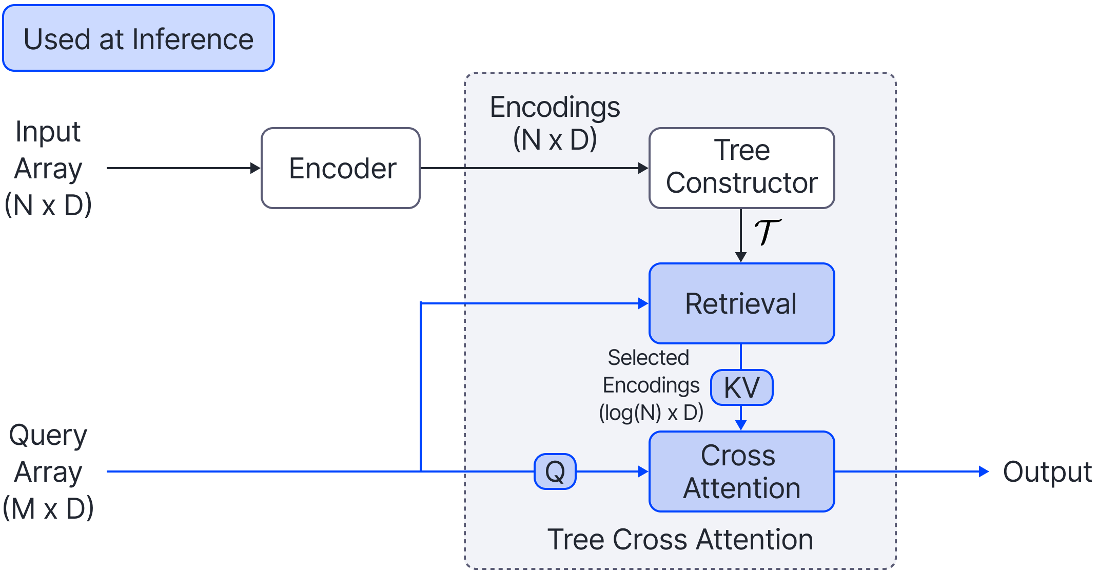
Figure 1: Architecture Diagram of ReTreever. Input Array comprises a set of $N$ context tokens which are fed through an encoder to compute a set of context encodings. Query Array denotes a batch of $M$ query feature vectors. Tree Cross Attention organizes the encodings and constructs a tree $\mathcal{T}$. At inference time, given a query feature vector, a logarithmic-sized subset of nodes (encodings) is retrieved from the tree $\mathcal{T}$. The query feature vector retrieves information from the subset of encodings via Cross Attention and makes a prediction.

We propose Tree Cross Attention (TCA), a token-efficient variant of Cross Attention. Tree Cross Attention is composed of three phases: (1) Tree Construction, (2) Retrieval, and (3) Cross Attention. In the Tree Construction phase ($\mathbb{R}^{N\times D}\rightarrow\mathcal{T}$), TCA organizes the context tokens ($\mathbb{R}^{N\times D}$) into a tree structure $(\mathcal{T})$ such that the context tokens are the leaves in the tree. The internal (i.e., non-leaf) nodes of the tree summarise the information in its subtree. Notably, this phase only needs to be performed once for a set of context tokens.

The Retrieval and Cross Attention is performed multiple times at inference time. During the Retrieval phase ($\mathcal{T}\times\mathbb{R}^{D}\rightarrow\mathbb{R}^{\mathcal{O}(\log(N))\times D}$), the model retrieves a logarithmic-sized selected subset of nodes $(\mathbb{S})$ from the tree using a query feature vector $q\in\mathbb{R}^{D}$ (or a batch of query feature vectors $\mathbb{R}^{M\times D})$. Afterwards, Cross Attention ($\mathbb{R}^{\mathcal{O}(\log(N))\times D}\times\mathbb{R}^{D}\rightarrow\mathbb{R}^{D}$) is performed by retrieving the information from the subset of nodes with the query feature vector. The overall complexity of inference is $\mathcal{O}(\log(N))$ per query feature vector. We detail these phases fully in the below subsections.

After describing the phases of TCA, we introduce ReTreever, a general architecture for token-efficient inference. Figure 1 illustrates the architecture of Tree Cross Attention and ReTreever.

3.1 Tree Construction

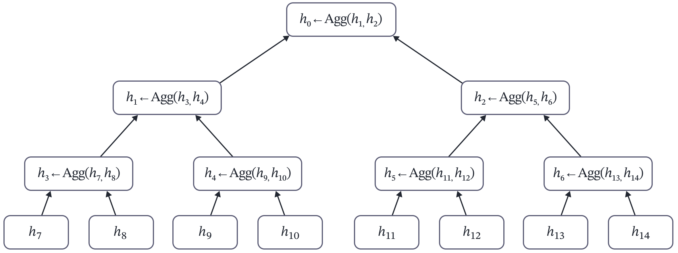
Figure 2: Diagram of the aggregation procedure performed during the Tree Construction phase. The aggregation procedure is performed bottom-up beginning from the parents of the leaves and ending at the root of the tree. The complexity of this procedure is $\mathcal{O}(N)$ but this only needs to be performed once for a set of context tokens. Compared to the cost of performing multiple predictions, the one-time cost of the aggregation process is minor.

The tokens are organized in a tree $\mathcal{T}$ such that the leaves of the tree consist of all the tokens. The internal nodes (i.e., non-leaf nodes) summarise the information of the nodes in their subtree. The information stored in a node has two specific desideratas, summarising the information in its subtree needed for performing (1) predictions and (2) retrieval (i.e., finding the specific nodes in its subtree relevant for the query feature vector).

The method of organizing the data in the tree is flexible and can be done either with prior knowledge of the structure of the data, with simple heuristics, or potentially learned. For example, heuristics used to organize the data in traditional tree algorithms can be used to organize the data, e.g., ball-tree (Omohundro,, 1989) or k-d tree (Cormen et al.,, 2006).

After organizing the data in the tree, an aggregator function $\mathrm{Agg}:\mathcal{P}(\mathbb{R}^{d})\rightarrow\mathbb{R}^{d}$ (where $\mathcal{P}$ denotes the power set) is used to aggregate the information of the tokens. Starting from the parent nodes of the leaves of the tree, the following aggregation procedure is performed bottom-up until the root of the tree: $h_{v}=\mathrm{Agg}(\{h_{u}|u\in\mathbb{C}_{v}\})$ where $\mathbb{C}_{v}$ denote the set of children nodes of a node $v$ and $h_{v}$ denote the vector representing the node. Figure 2 illustrates the aggregation process.

In our experiments, we consider a balanced binary tree. To organize the data, we use a k-d tree. During their construction, k-d trees select an axis and split the data evenly according to the median. To ensure the tree is perfectly balanced, padding tokens are added such that the values are masked during computation. Notably, these padding nodes are less than the number of tokens. As such, it does not affect the big-O complexity.

3.2 Retrieval

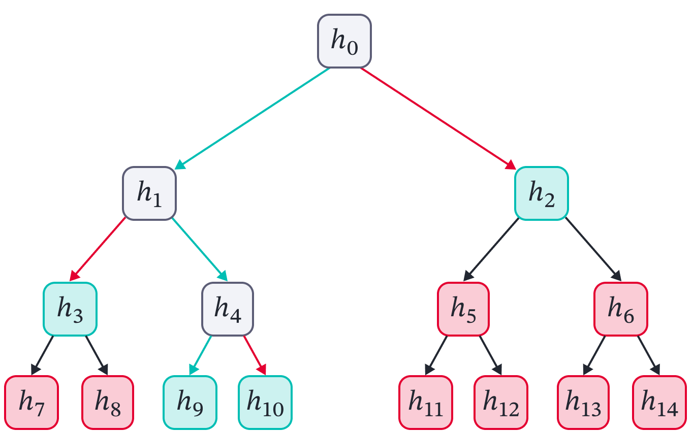
Figure 3: Example result of a Retrieval phase. The policy creates a path from the tree’s root to its leaves, selecting a subset of nodes: the terminal leaves in the path and the highest-level unexplored ancestors of the other leaves. The green arrows represent the path (actions) chosen by the policy $\pi$. The red arrows represent the actions rejected by the policy. The green nodes denote the subset of nodes selected, i.e., $\mathbb{S}=\{h_{2},h_{3},h_{9},h_{10}\}$. The grey nodes denote nodes that were explored at some point but not selected. The red nodes denote the nodes that were not explored or selected.

Algorithm 1 Retrieval

Tree Structure ($\mathcal{T}$), policy ($\pi_{\theta}$), and query feature vector $q$

Set of selected nodes ($\mathbb{S}$)

$v\leftarrow\mathrm{Root}(\mathcal{T})$

$\mathbb{S}\leftarrow\emptyset$

while $v$ is not leaf do

     $v^{\prime}\sim\pi_{\theta}(a|\mathbb{S},\mathbb{C}_{v},q)$ where $a\in\mathbb{C}_{v}$

     $\mathbb{S}\leftarrow\mathbb{S}\cup(\mathbb{C}_{v}\backslash v^{\prime})$ $\triangleright$ $\mathbb{C}_{v}$ denotes children nodes of $v$

     $v\leftarrow v^{\prime}$

end while

$\mathbb{S}\leftarrow\mathbb{S}\cup v$

To learn informative internal node embeddings for retrieval, we leverage a policy $\pi$ learned via Reinforcement Learning for retrieving a subset of nodes from the tree. Algorithm 1 describes the process of retrieving the set of selected nodes $\mathbb{S}$ from the tree $\mathcal{T}$. Figure 3 illustrates an example of the result of this phase. Figures 7 to 11 in the Appendix illustrate a step-by-step example of the retrieval described in Algorithm 1.

$v$ denotes the node of the tree currently being explored. At the start of the search, it is initialized as $v\leftarrow\mathrm{Root}(\mathcal{T})$. The policy’s state is the set of selected nodes $\mathbb{S}$, the set of children nodes of the current node being explored $\mathbb{C}_{v}$, and the query feature vector $q$, i.e., $s=(\mathbb{S},\mathbb{C}_{v},q)$. Starting from the root, the policy selects one of the children nodes, i.e., $v^{\prime}\sim\pi_{\theta}(a|\mathbb{S},\mathbb{C}_{v},q)$ where $a\in\mathbb{C}_{v}$, to further explore for more detailed information retrieval. The nodes that are not being further explored are added to the set of selected nodes $\mathbb{S}\leftarrow\mathbb{S}\cup(\mathbb{C}_{v}\backslash v^{\prime})$. Afterwards, $v$ is updated ($v\leftarrow v^{\prime}$) with the new node and the process is repeated until $v$ is a leaf node (i.e., the search is complete). Since the height of a balanced tree is $\mathcal{O}(\mathcal{\log(N)})$, as such, the number of nodes that are explored and retrieved is logarithmic: $||\mathbb{S}||=\mathcal{O}(\log(N))$.

3.3 Cross Attention

The retrieved set of nodes ($\mathbb{S}$) is used as input for Cross Attention alongside the query feature vector $q$. Since $||\mathbb{S}||=\mathcal{O}(\log(N))$, this results in a Cross Attention with overall logarithmic complexity $\mathcal{O}(\log(N))$ complexity per query feature vector. In contrast, applying Cross Attention to the full set of tokens has a linear complexity $\mathcal{O}(N)$. Notably, the set of nodes $\mathbb{S}$ has a full receptive field of the entire set of tokens, i.e., either a token is part of the selected set of nodes or is a descendant (in the tree) of one of the selected nodes.

3.4 ReTreever: Retrieval via Tree Cross Attention

In this section, we propose ReTreever (Figure 1), a general-purpose model that achieves token-efficient inference by leveraging Tree Cross Attention. The architecture is similar in style to Perceiver IO’s (Figure 5 in the Appendix).

In the case of Perceiver IO, the model is composed of (1) an iterative attention encoder ($\mathbb{R}^{N\times D}\rightarrow\mathbb{R}^{L\times D}$) which compresses the information into a smaller fixed-sized $L$ set of latent tokens and (2) a Cross Attention module used during inference for performing information retrieval from the set of latent tokens. As a result, Perceiver IO’s inference complexity is $\mathcal{O}(L)$.

In contrast, ReTreever is composed of (1) an encoder ($\mathbb{R}^{N\times D}\rightarrow\mathbb{R}^{N\times D}$) and (2) a Tree Cross Attention (TCA) module used during inference for performing information retrieval from a tree structure. Unlike Perceiver IO which compresses information via a specialized encoder to achieve efficient inference, ReTreever’s inference is token-efficient irrespective of the encoder, scaling logarithmically $\mathcal{O}(\log(N))$ with the number of tokens. As such, the choice of encoder is flexible and can be, for example, a Transformer Encoder or efficient versions such as Linformer, ChordMixer, etc.

3.5 Training Objective

The objective ReTreever optimises consists of three components with hyperparameters $\lambda_{CA}$ and $\lambda_{RL}$, denoting the weight of the terms:

$$\mathcal{L}_{ReTreever}=\mathcal{L}_{TCA}+\lambda_{RL}\mathcal{L}_{RL}+\lambda_{CA}\mathcal{L}_{CA}$$

$L_{TCA}$ aims to tackle the first desiderata, i.e., learning node representations in the tree that summarise the relevant information in its subtree for making good predictions.

$$\mathcal{L}_{TCA}=\mathrm{Loss}(\mathrm{CrossAttention}(x,\mathbb{S}),y)$$

$\mathcal{L}_{RL}$ tackles the second desiderata, i.e., learning internal node representations for retrieval (the RL policy $\pi$) within the tree structure.

$$\mathcal{L}_{RL}=\sum_{t=0}^{\log(N)-1}\left[\mathcal{R}\log\pi_{\theta}(a_{t}|s_{t})+\alpha\mathcal{H}[\pi_{\theta}(\cdot|s_{t})]\right]$$

The horizon is the height of the tree $\log(N)$, $\mathcal{H}$ denotes entropy, and $\mathcal{R}$ denotes the reward/objective we want ReTreever to maximise. Typically this reward corresponds to the negative TCA loss $\mathcal{R}=-\mathcal{L}_{TCA}$, e.g., Negative MSE, Log-Likelihood, and Negative Cross Entropy for regression, uncertainty estimation, and classification tasks, respectively. However, crucially, the reward does not need to be differentiable. As such, $\mathcal{R}$ can also be an objective we are typically not able to optimize directly via gradient descent, e.g., accuracy for classification tasks ($\mathcal{R}=1$ for correct classification and $\mathcal{R}=0$ for incorrect classification).

Lastly, to improve the early stages of training and encourage TCA to learn good node representations, $\mathcal{L}_{CA}$ is included:

$$\mathcal{L}_{CA}=\mathrm{Loss}(\mathrm{CrossAttention}(x,\mathrm{Leaves(\mathcal{T})}),y)$$

4 Experiments

Our objective in the experiments is: (1) Compare Tree Cross Attention (TCA) with Cross Attention in terms of the number of tokens used and the performance. We answer this in two ways: (i) by comparing Tree Cross Attention and Cross Attention directly on a memory retrieval task and (ii) by comparing our proposed model ReTreever which uses TCA with models which use Cross Attention. (2) Compare the performances of ReTreever and Perceiver while using the same number of tokens. In terms of analyses, we aim to: (3) Highlight how ReTreever and TCA can optimize for non-differentiable objectives using $\mathcal{L}_{RL}$, improving performance. (4) Show the importance of the different loss terms in the training objective. (5) Empirically show the rate at which Cross Attention and TCA memory grow with respect to the number of tokens.

To tackle those objectives, we consider benchmarks for classification (Copy Task, Human Activity) and uncertainty estimation settings (GP Regression and Image Completion). Our focus is on (1) comparing Tree Cross Attention with Cross Attention, and (2) comparing ReTreever with general-purpose models (i) Perceiver IO for the same number of latents and (ii) Transformer (Encoder) + Cross Attention. Full details regarding the hyperparameters are included in the appendix.

For completeness, in the appendix, we include the results for many other baselines (including recent state-of-the-art methods) for the problem settings considered in this paper. The results show the baseline Transformer + Cross Attention achieves results competitive with prior state-of-the-art. Specifically, we compared against the following baselines for GP Regression and Image Completion: LBANPs (Feng et al., 2023a, ), TNPs (Nguyen and Grover,, 2022), NPs (Garnelo et al., 2018b, ), BNPs (Lee et al.,, 2020), CNPs (Garnelo et al., 2018a, ), CANPs (Kim et al.,, 2019), ANPs (Kim et al.,, 2019), and BANPs (Lee et al.,, 2020). We compared against the following baselines for Human Activity: SeFT (Horn et al.,, 2020), RNN-Decay (Che et al.,, 2018), IP-Nets (Shukla and Marlin,, 2019), L-ODE-RNN (Chen et al.,, 2018), L-ODE-ODE (Rubanova et al.,, 2019), and mTAND-Enc (Shukla and Marlin,, 2021). Additionally, we include results in the Appendix for Perceiver IO with a various number of latent tokens, showing Perceiver IO requires several times more tokens to achieve comparable performance to ReTreever.

4.1 Copy Task

We first verify the ability of Cross Attention and Tree Cross Attention (TCA) to perform retrieval. The models are provided with a sequence of length $N=2^{k}$, beginning with a [BOS] (Beginning of Sequence) token, followed by a randomly generated palindrome comprising of $2^{k}-2$ digits, ending with a [EOS] (End of Sequence) token. The objective of the task is to predict the second half ($2^{k-1}$) of the sequence given the first half ($2^{k-1}$ tokens) of the sequence as context. To make a correct prediction for index $2^{k}-i$ (where $0<i\leq 2^{k-1}$), the model must retrieve information from its input/context sequence at index $i+1$. The model is evaluated on its accuracy on $3200$ randomly generated test sequences. As a point of comparison, we include Random as a baseline, which makes random predictions sampled from the set of digits ($0-9$), [EOS], and [BOS] tokens.

Results. We found that both Cross Attention and Tree Cross Attention were able to solve this task perfectly (Table 1). In comparison, TCA requires $\sim 50\times$ fewer tokens than Cross Attention. Furthermore, we found that Perceiver IO’s performance was dismal ($15.2\pm 0.0\%$ accuracy at $N=256$), further dropping in performance as the length of the sequence increased. This result is expected as Perceiver IO aims to compress all the relevant information for any predictions into a small fixed-sized set of latents. However, all the tokens are relevant depending on the queried index. As such, methods which distill information to a lower dimensional space are insufficient. In contrast, TCA performs tree-based memory retrieval, selectively retrieving a small subset of tokens for predictions. As such, TCA is able to solve the task perfectly while using the same number of tokens as Perceiver.

Method $N=256$ $N=512$ $N=1024$ % Tokens Accuracy % Tokens Accuracy % Tokens Accuracy Cross Attention $100.0\%$ $\mathbf{100.0\pm 0.0}$ $100.0\%$ $\mathbf{100.0\pm 0.0}$ $100.0\%$ $\mathbf{99.9\pm 0.2}$ Random — $8.3\pm 0.0$ — $8.3\pm 0.0$ — $8.3\pm 0.0$ Perceiver IO $\mathbf{6.3\%}$ $15.2\pm 0.0$ $\mathbf{3.5\%}$ $13.4\pm 0.2$ $\mathbf{2.0\%}$ $11.6\pm 0.4$ TCA $\mathbf{6.3\%}$ $\mathbf{100.0\pm 0.0}$ $\mathbf{3.5\%}$ $\mathbf{100.0\pm 0.0}$ $\mathbf{2.0\%}$ $\mathbf{99.6\pm 0.6}$

Table 1: Copy Task Results with accuracy (higher is better) and $\%$ tokens (lower is better) metrics.

4.2 Uncertainty Estimation: GP Regression and Image Completion

We evaluate ReTreever on popular uncertainty estimation settings used in (Conditional) Neural Processes literature and which have been benchmarked extensively (Table 7 in Appendix)  (Garnelo et al., 2018a, ; Garnelo et al., 2018b, ; Kim et al.,, 2019; Lee et al.,, 2020; Nguyen and Grover,, 2022; Feng et al., 2023a, ; Feng et al., 2023b, ).

4.2.1 GP Regression

The goal of the GP Regression task is to model an unknown function $f$ given $N$ points. During training, the functions are sampled from a GP prior with an RBF kernel $f_{i}\sim GP(m,k)$ where $m(x)=0$ and $k(x,x^{\prime})=\sigma_{f}^{2}\exp(-\frac{(x-x^{\prime})^{2}}{2l^{2}})$. The hyperparameters of the kernel are randomly sampled according to $l\sim\mathcal{U}[0.6,1.0)$, $\sigma_{f}\sim\mathcal{U}[0.1,1.0)$, $N\sim\mathcal{U}[3,47)$, and $M\sim\mathcal{U}[3,50-N)$. After training, the models are evaluated according to the log-likelihood of functions sampled from GPs with RBF and Matern 5/2 kernels.

Method	$\%$ Tokens	RBF	Matern 5/2
Transformer + Cross Attention	$100\%$	$\mathbf{1.35\pm 0.02}$	$\mathbf{0.91\pm 0.02}$
ReTreever-Full	$100\%$	$\mathbf{1.33\pm 0.02}$	$\mathbf{0.90\pm 0.01}$
Perceiver IO	$\mathbf{14.9\%}$	$1.06\pm 0.05$	$0.58\pm 0.05$
Perceiver IO ($L=32$)	$68.0\%$	1.25 ± 0.04	0.78 ± 0.05
ReTreever	$\mathbf{14.9\%}$	$\mathbf{1.25\pm 0.02}$	$\mathbf{0.81\pm 0.02}$

Table 2: 1-D Meta-Regression Experiments with log-likelihood (higher is better) and $\%$ tokens (lower is better) metrics.

Results. In Table 2, we see that ReTreever ($1.25\pm 0.02$) outperforms Perceiver IO ($1.06\pm 0.05$) by a large margin while using the same number of tokens for inference. To see how many latents Perceiver IO would need to achieve performance comparable to ReTreever, we varied the number of latents (see Appendix Table 7 for full results). We found that Perceiver IO needed $\sim 4.6\times$ the number of tokens to achieve comparable performance.

4.2.2 Image Completion

The goal of the Image Completion task is to make predictions for the pixels of an image given a random subset of pixels of an image. The CelebA dataset comprises coloured images of celebrity faces. The images are downsized to size $32\times 32$. The $x$ values are rescaled to be between [-1, 1] and the y values to be between [-0.5, 0.5]. The number of pixels are sampled according to $N\sim\mathcal{U}[3,197)$ and $M\sim\mathcal{U}[3,200-N)$.

Method	$\%$ Tokens	CelebA
Transformer + Cross Attention	$100\%$	$\mathbf{3.88\pm 0.01}$
ReTreever-Full	$100\%$	$3.77\pm 0.01$
Perceiver IO	$\mathbf{4.6\%}$	$3.20\pm 0.01$
ReTreever-Random	$\mathbf{4.6\%}$	$3.12\pm 0.02$
ReTreever-KD-$x_{0}$	$\mathbf{4.6\%}$	$\mathbf{3.50\pm 0.02}$
ReTreever-KD-$x_{1}$	$\mathbf{4.6\%}$	$\mathbf{3.52\pm 0.01}$
ReTreever-KD-RP	$\mathbf{4.6\%}$	$\mathbf{3.51\pm 0.01}$

Table 3: Image Completion Experiments. The methods are evaluated according to the log-likelihood (higher is better) and $\%$ tokens (lower is better) metrics.

Unlike sequential data where there is a clear axis (e.g., index or timestamp) in which to split the data when constructing the k-d tree, it is less clear which axis to split 2-D image pixel data. In this experiment, we compare the performance of ReTreever with various heuristics for constructing the tree (1) organized randomly (ReTreever-Random) without a k-d tree, (2) constructing the k-d tree according to the first index $x_{0}$ of the image data (ReTreever-KD-$x_{0}$), (3) constructing the k-d tree via the second index $x_{1}$ of the image data (ReTreever-KD-$x_{1}$), and (4) constructing the k-d tree using the value after a Random Projection (ReTreever-KD-RP). ReTreever-KD-RP generates a fixed random matrix $w\in\mathbb{R}^{dim(x)\times 1}$ and splits the context tokens in the tree according to $w^{T}x$.

Results. In Table 3, we see that ReTreever-Random performs close to Perceiver. The performance of ReTreever-Random is expected as the structure of the tree is uninformative for search. By leveraging any of the heuristics, ReTreever-KD-$x_{0}$ ($3.50\pm 0.02$), ReTreever-KD-$x_{1}$ ($3.52\pm 0.01$), and ReTreever-KD-RP ($3.51\pm 0.01$) all significantly outperform Perceiver ($3.20\pm 0.01$). Notably, ReTreever uses $\sim 21\times$ fewer tokens than Transformer + Cross Attention. Additional results on the EMNIST dataset are included in the appendix which show similar results.

4.2.3 ReTreever-Full

ReTreever leverages RL to learn good node representations for informative retrieval. However, ReTreever is not limited to only using the learned policy for retrieval at inference time. For example, instead of retrieving a subset of the nodes according to a policy, we can choose to retrieve all the leaves of the tree "ReTreever-Full" (see Table 2 and 3).

Results. On CelebA and GP Regression, we see that ReTreever-Full achieves performance close to state-of-the-art. For example, on CelebA, ReTreever-Full achieves $3.77\pm 0.01$, and Transformer + Cross Attention achieves $3.88\pm 0.01$. On GP, ReTreever-Full achieves $1.33\pm 0.02$, and Transformer + Cross Attention achieves $1.35\pm 0.02$. In contrast, ReTreever achieves significantly lower results. The performance gap between ReTreever and ReTreever-Full suggests that the performance of ReTreever can vary depending on the number of nodes (tokens) selected from the tree. As such, an interesting future direction is the design of alternative methods for selecting subsets of nodes.

4.3 Time Series: Human Activity

The human activity dataset consists of 3D positions of the waist, chest, and ankles (12 features) collected from five individuals performing various activities such as walking, lying, and standing. We follow prior works preprocessing steps, constructing a dataset of $6,554$ sequences with $50$ time points. The objective of this task is to classify each time point into one of eleven types of activities.

Model	$\%$ Tokens	Accuracy
Transformer + Cross Attention	$100\%$	$\mathbf{89.1\pm 1.3}$
Perceiver IO	$\mathbf{14\%}$	$87.6\pm 0.3$
ReTreever	$\mathbf{14\%}$	$\mathbf{88.9\pm 0.4}$

Table 4: Human Activity Experiments with accuracy (higher is better) and $\%$ tokens (lower is better) metrics.

Results. Table 4 show similar conclusions as our prior experiments. (1) ReTreever performs comparable to Transformer + Cross Attention, requiring far fewer tokens ($86\%$ less), and (2) ReTreever outperforms Perceiver IO significantly while using the same number of tokens.

4.4 Analyses

Memory Usage. Tree Cross Attention’s memory usage (Figure 4 (left)) is significantly more efficient than Cross Attention, growing logarithmically in the number of tokens compared to linearly.

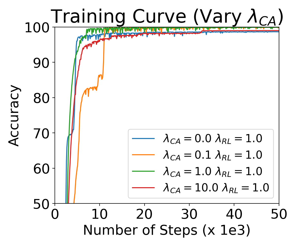
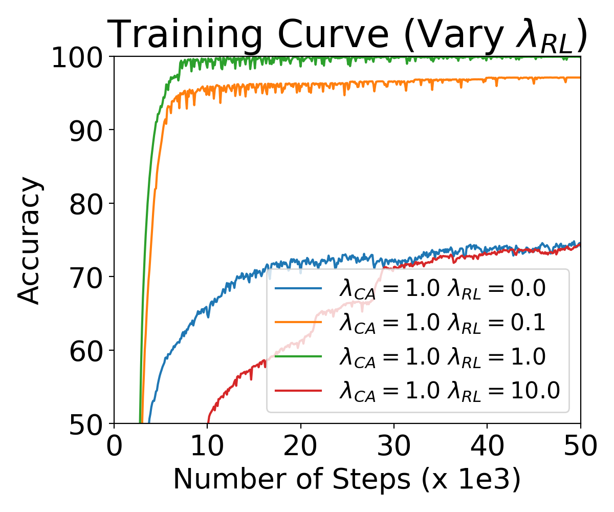
Figure 4: Memory Usage Plot comparing the rate in which memory usage grows at inference time relative to the number of tokens. We see that CrossAttention grows linearly with the number of tokens. TreeCrossAttention grows logarithmically, which is barely noticeable.

Importance of the different loss terms $\lambda_{CA}$ and $\lambda_{RL}$. Figure 4 (right) shows that the weight of the RL loss term is crucial to achieving good performance. $\lambda_{RL}=1.0$ performed the best. If the weight of the term is too small $\lambda_{RL}\in\{0.0,0.1\}$ or too large $\lambda_{RL}=10.0$, the model is unable to solve the task. Figure 4 (middle) shows that the weight of the Cross Attention loss term improves the stability of the training, particularly in the early stages. Setting $\lambda_{CA}=1.0$ performed the best. Setting too small values for $\lambda_{CA}\in\{0.0,0.1\}$ causes some erraticness in the early stages of training. Setting too large of a value $\lambda_{CA}=10.0$ slows down training.

Method $N=256$ $N=512$ $N=1024$ % Tokens Accuracy % Tokens Accuracy % Tokens Accuracy TCA (Acc) $\mathbf{6.3\%}$ $\mathbf{100.0\pm 0.0}$ $\mathbf{3.5\%}$ $\mathbf{100.0\pm 0.0}$ $\mathbf{2.0\%}$ $\mathbf{99.6\pm 0.6}$ TCA (Neg. CE) $\mathbf{6.3\%}$ $\mathbf{99.8\pm 0.3}$ $\mathbf{3.5\%}$ $95.5\pm 3.8$ $\mathbf{2.0\%}$ $80.3\pm 14.8$

Table 5: Comparison of Accuracy and Negative Cross Entropy as the reward.

Optimising non-differentiable objectives using $\mathcal{L}_{RL}$. In classification, typically, accuracy is the metric we truly care about. However, accuracy is a non-differentiable objective, so instead in deep learning, we often use cross entropy so we can optimize the model’s parameters via gradient descent. However, in the case of RL, the reward does not need to be differentiable. As such, we compare the performance of ReTreever when optimizing for the accuracy and the negative cross entropy. Table 5 shows that accuracy as the RL reward improves upon using negative cross entropy. This is expected since (1) the metric we evaluate our model on is accuracy and not cross entropy, and (2) accuracy as a reward is simpler compared to negative cross entropy as a reward, making it easier for a policy to optimize. More specifically, a reward using accuracy as the metric is either: $\mathcal{R}=0$ for an incorrect prediction or $\mathcal{R}=1$ for a correct prediction. However, a reward based on cross entropy can have vastly different values for incorrect predictions.

5 Related Work

There have been a few works which have proposed to leverage a tree-based architecture (Tai et al.,, 2015; Nguyen et al.,, 2020; Madaan et al.,, 2023; Wang et al.,, 2019) for attention, the closest of which to our work is Treeformer (Madaan et al.,, 2023). Unlike prior works (including Treeformer) which focused on replacing self-attention in transformers with tree-based attention, in our work, we focus on replacing cross attention with a tree-based cross attention mechanism for efficient memory retrieval for inferences. Furthermore, Treeformer (1) uses a decision tree to find the leaf that closest resembles the query feature vector, (2) TF-A has a partial receptive field comprising only the tokens in the selected leaf, and (3) TF-A has a worst-case linear complexity in the number of tokens per query. In contrast, TCA (1) learns a policy to select a subset of nodes, (2) retrieves a subset of nodes with a full receptive field, and (3) has a guaranteed logarithmic complexity.

As trees are a form of graphs, Tree Cross Attention bears a resemblance to Graph Neural Networks (GNNs). The objectives, however, of GNNs and TCA are different. In GNNs, the objective is to perform edge, node, or graph predictions. However, the goal of TCA is to search the tree for a subset of nodes that is relevant for a query. Furthermore, unlike GNNs which typically consider the tokens to correspond one-to-one with nodes of the graph, TCA only considers the leaves of the tree to be tokens. We refer the reader to surveys on GNNs (Wu et al.,, 2020; Thomas et al.,, 2023).

6 Conclusion

In this work, we proposed Tree Cross Attention (TCA), a variant of Cross Attention that only requires a logarithmic $\mathcal{O}(\log(N))$ number of tokens when performing inferences. By leveraging RL, TCA can optimize non-differentiable objectives such as accuracy. Building on TCA, we introduced ReTreever, a flexible architecture for token-efficient inference. We evaluate across various classification and uncertainty prediction tasks, showing (1) TCA achieves performance comparable to Cross Attention, (2) ReTreever outperforms Perceiver IO while using the same number of tokens for inference, and (3) TCA’s memory usage scales logarithmically with respect to the number of tokens compared to Cross Attention which scales linearly.

Appendix A Appendix: Illustrations

A.1 Baseline Architectures

Figures 5 and 6 illustrate the difference in architectures between the main baselines considered in the paper. Transformer + Cross Attention is composed of a Transformer encoder ($\mathbb{R}^{N\times D}\rightarrow\mathbb{R}^{N\times D}$) and a Cross Attention module ($\mathbb{R}^{M\times D}\times\mathbb{R}^{N\times D}\rightarrow\mathbb{R}^{M\times D}$). Perceiver IO is composed of an iterative attention encoder ($\mathbb{R}^{N\times D}\rightarrow\mathbb{R}^{L\times D}$) and a Cross Attention module ($\mathbb{R}^{M\times D}\times\mathbb{R}^{L\times D}\rightarrow\mathbb{R}^{M\times D}$). In contrast, ReTreever (Figure 1) is composed of a flexible encoder ($\mathbb{R}^{N\times D}\rightarrow\mathbb{R}^{N\times D}$) and a Tree Cross Attention module.

Empirically, we showed that Transformer + Cross Attention achieves good performance. However, its Cross Attention is inefficient due to retrieving from the full set of tokens. Notably, Perceiver IO achieves its inference-time efficiency by performing a compression via an iterative attention encoder. To achieve token-efficient inferences, the number of latents needs to be significantly less than the number of tokens originally, i.e., $L<<N$. However, this is not practical in hard problems since setting low values for $L$ results in significant information loss due to the latents being a bottleneck. In contrast, ReTreever is able to perform token-efficient inference while achieving better performance than Perceiver IO for the same number of tokens. ReTreever does this by using Tree Cross Attention to retrieve the necessary tokens, only needing a logarithmic number of tokens $\log(N)<<N$, making it efficient regardless of the encoder used. Crucially, this also means that ReTreever is more flexible with its encoder than Perceiver IO, allowing for customizing the kind of encoder depending on the setting.

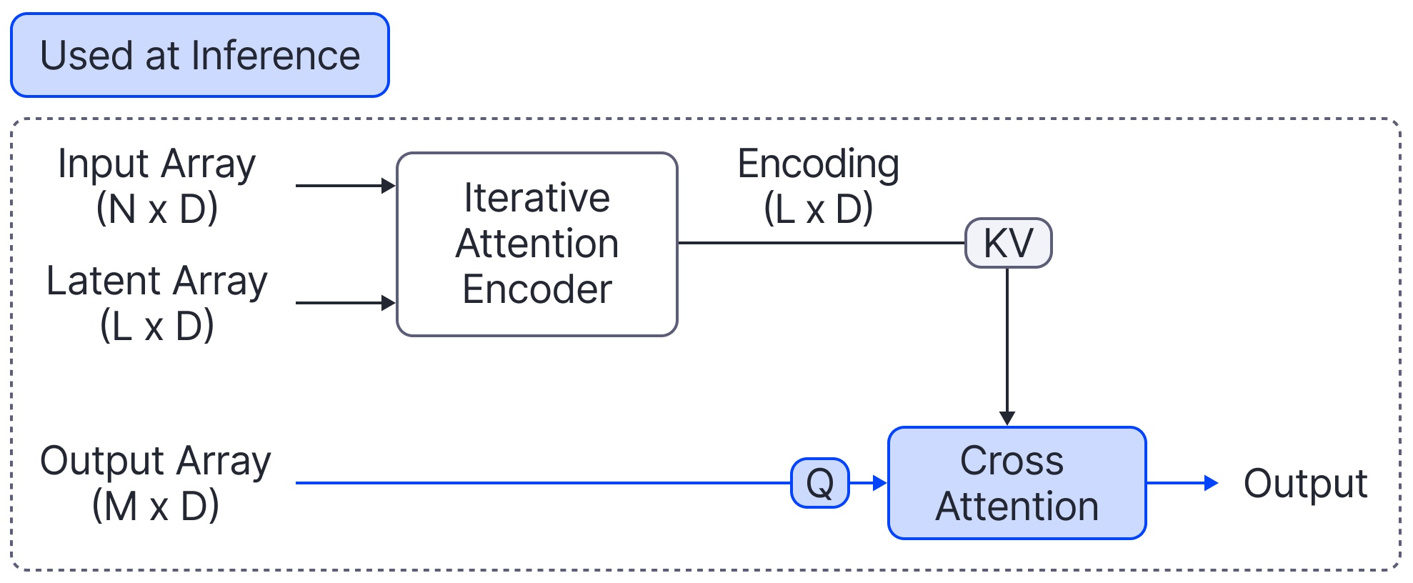
Figure 5: Architecture Diagram of Perceiver. The model is composed of an iterative attention encoder ($\mathbb{R}^{N\times D}\rightarrow\mathbb{R}^{L\times D}$) and a Cross Attention module ($\mathbb{R}^{M\times D}\times\mathbb{R}^{L\times D}\rightarrow\mathbb{R}^{M\times D}$).

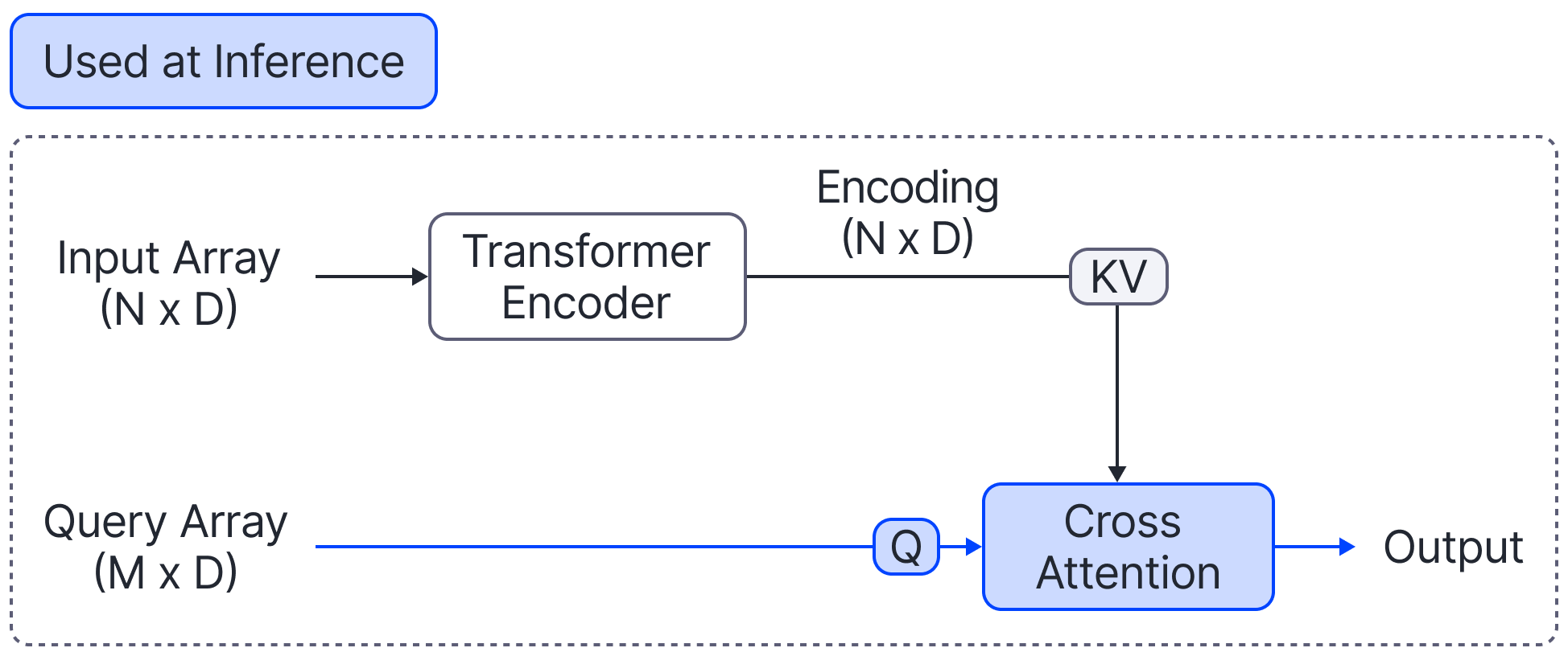
Figure 6: Architecture Diagram of Transformer + Cross Attention. The model is composed of a Transformer encoder ($\mathbb{R}^{N\times D}\rightarrow\mathbb{R}^{N\times D}$) and a Cross Attention module ($\mathbb{R}^{M\times D}\times\mathbb{R}^{N\times D}\rightarrow\mathbb{R}^{M\times D}$).

A.2 Example Retrieval

In Figures 7 to 11, we illustrate an example of the retrieval process described in Algorithm 1.

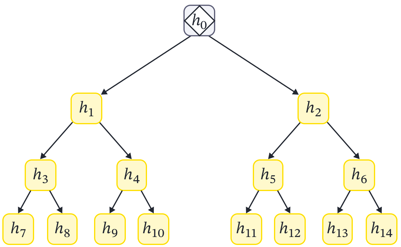
Figure 7: Example Retrieval Step 0 Illustration. The diamond icon on a node indicates the node that will be explored. The retrieval process begins at the root, i.e., $v\leftarrow 0$ where $0$ is the index of the root node. Yellow nodes denote the nodes that have yet to be explored and may be explored in the future. Grey nodes denote the nodes that are or have been explored but have not been added to the selected set $\mathbb{S}$. Red nodes denote the nodes that have not been explored and will not be explored in the future. Green nodes denote the subset of nodes selected, i.e., $\mathbb{S}$.

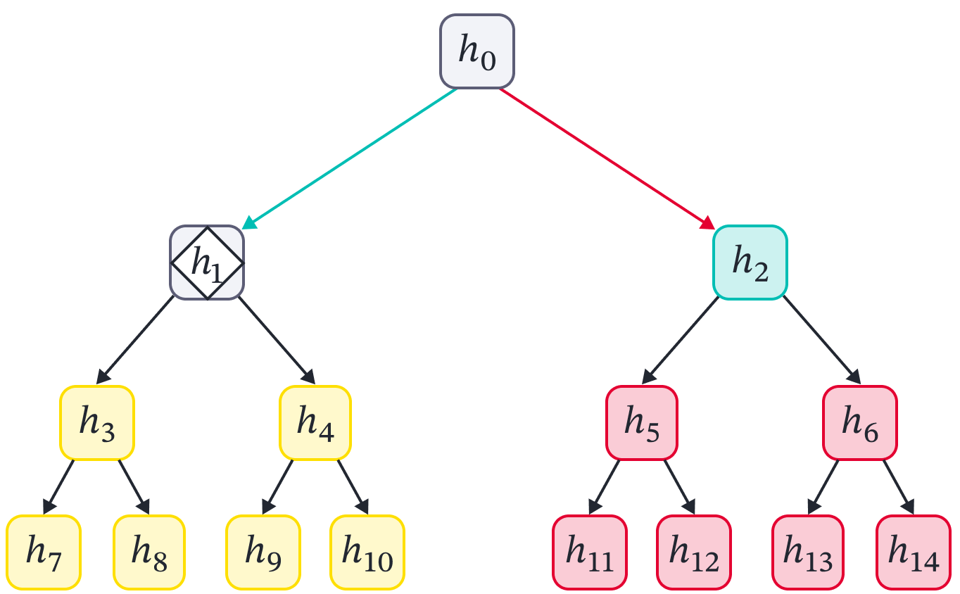
Figure 8: Example Retrieval Step 1 Illustration. Green arrows represent the path (actions) chosen by the policy $\pi$ for a query feature vector. Red arrows represent the actions rejected by the policy. The right child of $v=0$ was rejected, so it is added to the selected set $\mathbb{S}$. As a consequence, descendant nodes of $v$’s right child will never be explored, so they are coloured red in the diagram. Tentatively, $\mathbb{S}=\{h_{2}\}$. Because the policy selected the left child of $v=0$, we thus have $v\leftarrow 1$

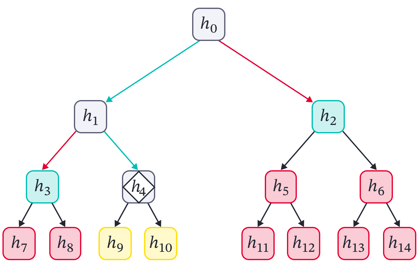
Figure 9: Example Retrieval Step 2 Illustration. The left child of $v=1$ is rejected this time, so it is added to the selected set $\mathbb{S}$ (green). Tentatively, $\mathbb{S}=\{h_{2},h_{3}\}$. Consequently, the descendant nodes of $v$’s left child will never be explored, so they are coloured red. Because the policy selected the right child of $v=1$, we thus have $v\leftarrow 4$.

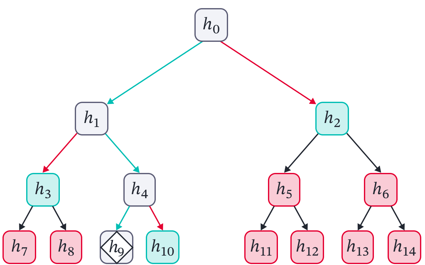
Figure 10: Example Retrieval Step 3 Illustration. The right child of $v=4$ is rejected this time, so it is added to the selected set $\mathbb{S}$. Tentatively, $\mathbb{S}=\{h_{2},h_{3},h_{10}\}$. The descendant nodes of $v$’s right child are to be coloured red, but there are none. Because the policy selected the left child of $v=4$, we thus have $v\leftarrow 9$

Figure 11: Example Retrieval Step 4 Illustration. $v=9$ is a leaf, so the tree search has reached its end. At the end of the tree search, we simply add the node to the selected set, resulting in $\mathbb{S}=\{h_{2},h_{3},h_{9},h_{10}\}$.

Appendix B Appendix: Additional Experiments and Analyses

In this section, we evaluate ReTreever with various baselines, including state-of-the-art methods. We show that a simple method like Transformer Encoder + Cross Attention can perform comparable to state-of-the-art. We further show that ReTreever achieves strong performance while requiring few tokens, outperforming Perceiver IO for the same number of tokens. We include additional results on another popular image completion dataset: EMNIST.

We also include the performance of Perceiver IO with various amounts of latents, showing that Perceiver IO requires significantly more tokens to achieve performance comparable to ReTreever.

B.1 Copy Task

Method	$N=128$
	% Tokens	Accuracy
Cross Attention	$100.0\%$	$\mathbf{100.0\pm 0.0}$
Random	—	$8.3\pm 0.0$
Perceiver IO	$\mathbf{2.0\%}$	$17.8\pm 0.0$
TCA (Acc)	$\mathbf{2.0\%}$	$\mathbf{100.0\pm 0.0}$
TCA (CE)	$\mathbf{2.0\%}$	$\mathbf{100.0\pm 0.0}$

Table 6: Copy Task Results with accuracy (higher is better) and $\%$ tokens (lower is better) metrics.

Results. In Table 6, we include additional results for the Copy Task where $N=128$. Similar to previous results, we see that Cross Attention and TCA are able to solve this task perfectly. In contrast, Perceiver IO is not able to solve this task for the same number of tokens.

B.2 Uncertainty Estimation: GP Regression

Method	$\%$ Tokens	RBF	Matern 5/2
CNP (Garnelo et al., 2018a, )	—	0.26 ± 0.02	0.04 ± 0.02
CANP (Kim et al.,, 2019)	—	0.79 ± 0.00	0.62 ± 0.00
NP (Garnelo et al., 2018b, )	—	0.27 ± 0.01	0.07 ± 0.01
ANP (Kim et al.,, 2019)	—	0.81 ± 0.00	0.63 ± 0.00
BNP (Lee et al.,, 2020)	—	0.38 ± 0.02	0.18 ± 0.02
BANP (Lee et al.,, 2020)	—	0.82 ± 0.01	0.66 ± 0.00
TNP-D (Nguyen and Grover,, 2022)	—	$\mathbf{1.39\pm 0.00}$	$\mathbf{0.95\pm 0.01}$
LBANP (Feng et al., 2023a, )	—	1.27 ± 0.02	0.85 ± 0.02
CMANP (Feng et al., 2023b, )	—	1.24 ± 0.02	0.80 ± 0.01
Perceiver IO ($L=4$)	$8.5\%$	1.02 ± 0.03	0.56 ± 0.03
Perceiver IO ($L=8$)	$17.0\%$	1.13 ± 0.03	0.65 ± 0.03
Perceiver IO ($L=16$)	$34.0\%$	1.22 ± 0.05	0.75 ± 0.06
Perceiver IO ($L=32$)	$68.0\%$	1.25 ± 0.04	0.78 ± 0.05
Perceiver IO ($L=64$)	$136.0\%$	1.30 ± 0.03	0.85 ± 0.02
Perceiver IO ($L=128$)	$272.0\%$	1.29 ± 0.04	0.84 ± 0.04
Transformer + Cross Attention	$100\%$	$\mathbf{1.35\pm 0.02}$	$\mathbf{0.91\pm 0.02}$
ReTreever-Full	$100\%$	$\mathbf{1.33\pm 0.02}$	$\mathbf{0.90\pm 0.01}$
Perceiver IO	$14.9\%$	1.06 ± 0.05	0.58 ± 0.05
ReTreever	$14.9\%$	1.25 ± 0.02	0.81 ± 0.02

Table 7: 1-D Meta-Regression Experiments with log-likelihood metric (higher is better).

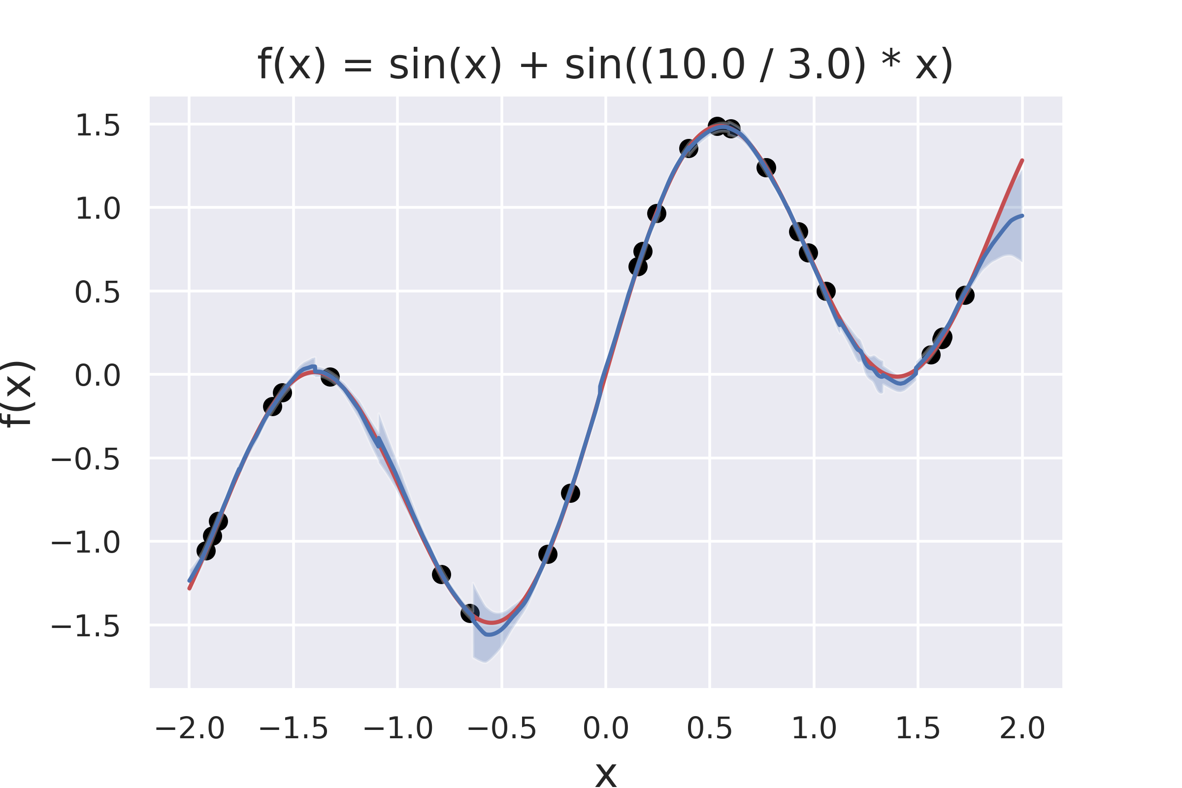
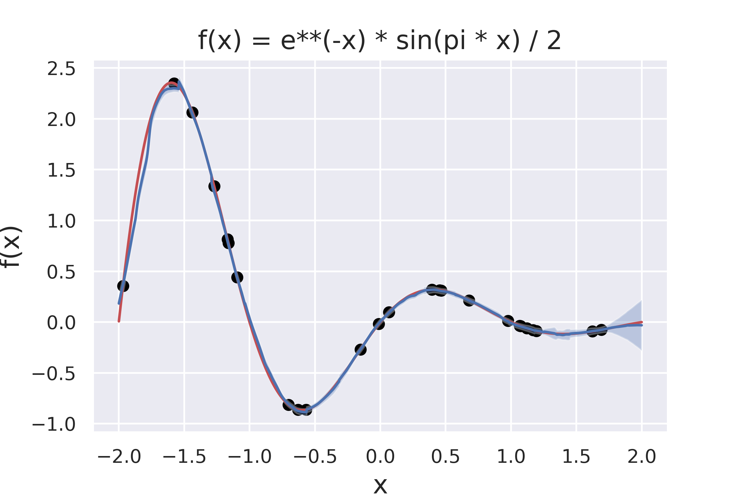
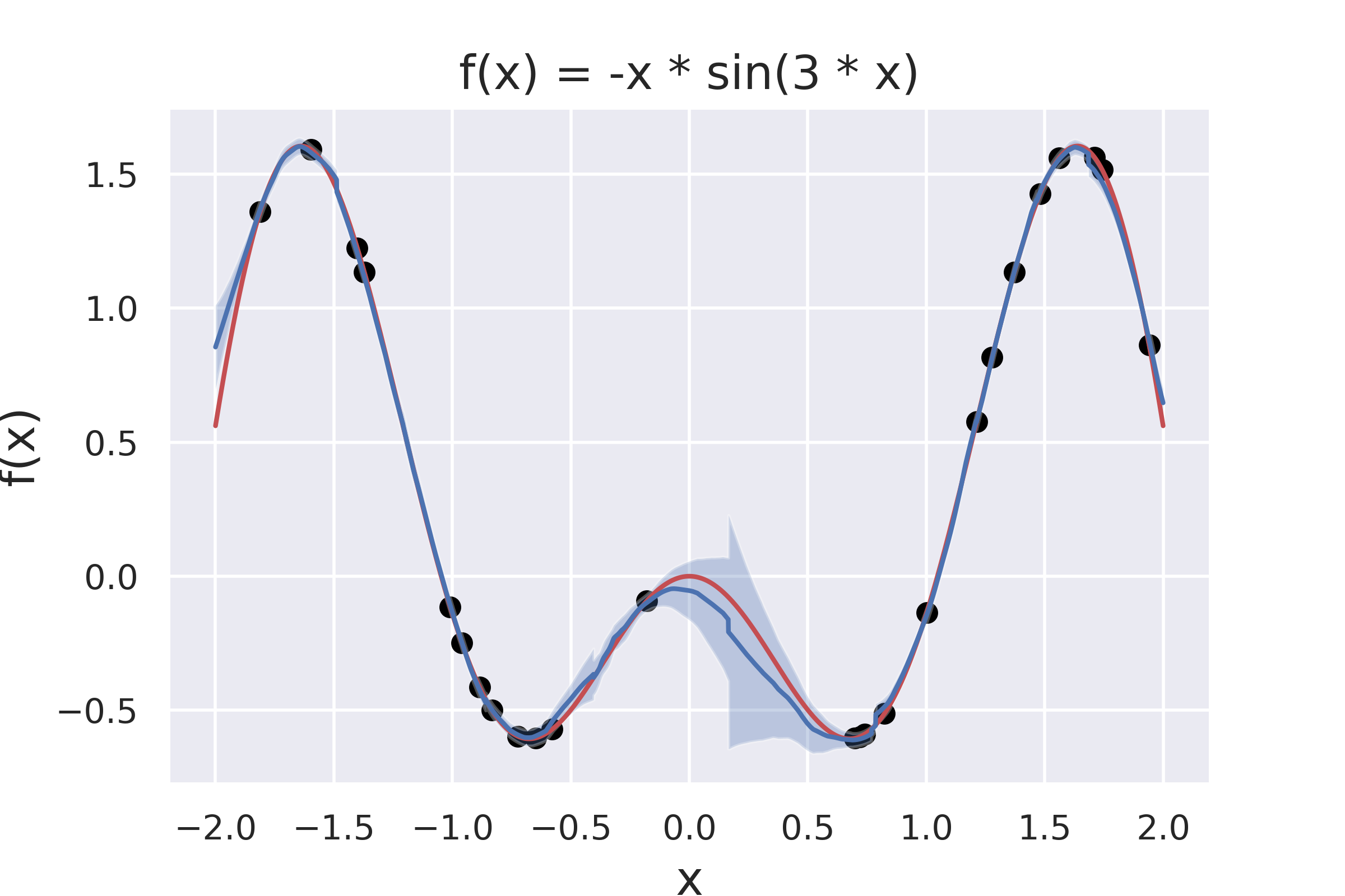
Figure 12: Visualizations of GP Regression

Results. In Table 7, we show results for all baselines on GP Regression. We see that Transformer + Cross Attention and ReTreever-Full perform comparable to the state-of-the-art, outperforming all Neural Process baselines except for TNP-D by a significant margin. We evaluated Perceiver IO with varying number of latents $L$. We see that Perceiver IO ($L=32$) uses $\sim 4.6\times$ the number of tokens to achieve performance comparable to ReTreever. Furthermore, ReTreever-Full outperforms Perceiver IO regardless of the number of tokens. ReTreever by itself already outperforms all NP baselines except for LBANP and TNP-D. Visualizations for different kinds of test functions are included in Figure 12.

B.3 Uncertainty Estimation: Image Completion

B.3.1 CelebA

Method	$\%$ Tokens	CelebA
CNP	—	2.15 ± 0.01
CANP	—	2.66 ± 0.01
NP	—	2.48 ± 0.02
ANP	—	2.90 ± 0.00
BNP	—	2.76 ± 0.01
BANP	—	3.09 ± 0.00
TNP-D	—	3.89 ± 0.01
LBANP (8)	—	3.50 ± 0.05
LBANP (128)	—	3.97 ± 0.02
CMANP	—	3.93 ± 0.05
Perceiver IO (8)	$4.1\%$	3.18 ± 0.03
Perceiver IO (16)	$8.1\%$	3.35 ± 0.02
Perceiver IO (32)	$16.2\%$	3.50 ± 0.02
Perceiver IO (64)	$32.5\%$	3.61 ± 0.03
Perceiver IO (128)	$65.0\%$	3.74 ± 0.02
Transformer + Cross Attention	$100\%$	$\mathbf{3.88\pm 0.01}$
ReTreever-Full	$100\%$	$3.77\pm 0.01$
Perceiver IO	$4.6\%$	$3.20\pm 0.01$
ReTreever-Random	$4.6\%$	$3.12\pm 0.02$
ReTreever-KD-$x_{0}$	$4.6\%$	$3.50\pm 0.02$
ReTreever-KD-$x_{1}$	$4.6\%$	$3.52\pm 0.01$
ReTreever-KD-RP	$4.6\%$	$3.51\pm 0.01$

Table 8: Image Completion Experiments. The methods are evaluated according to the log-likelihood (higher is better).

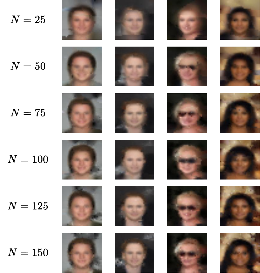
Figure 13: Visualizations of CelebA32

Results. In Table 8, we show results for all baselines on CelebA. We see that Transformer + Cross Attention achieves results competitive with the state-of-the-art. We further see that ReTreever-Full achieves performance close to that of state-of-the-art. We evaluated Perceiver IO with varying numbers of latents $L$. We see that Perceiver IO ($L=32$) uses $\sim 3.5\times$ the number of tokens to achieve performance comparable to the various ReTreever models. Visualizations are available in Figure 13.

B.3.2 EMNIST

Method	$\%$ Tokens	EMNIST
CNP	—	0.73 ± 0.00
CANP	—	0.94 ± 0.01
NP	—	0.79 ± 0.01
ANP	—	0.98 ± 0.00
BNP	—	0.88 ± 0.01
BANP	—	1.01 ± 0.00
TNP-D	—	1.46 ± 0.01
LBANP (8)	—	1.34 ± 0.01
LBANP (128)	—	1.39 ± 0.01
LBANP (128)	—	1.36 ± 0.01
CMANP	—	1.36 ± 0.01
Transformer + Cross Attention	$100\%$	$1.41\pm 0.00$
Perceiver IO	$4.6\%$	$1.25\pm 0.00$
ReTreever-Random	$4.6\%$	$1.26\pm 0.01$
ReTreever-KD-$x_{0}$	$4.6\%$	$1.30\pm 0.01$
ReTreever-KD-$x_{1}$	$4.6\%$	$1.26\pm 0.02$
ReTreever-KD-RP	$4.6\%$	$1.29\pm 0.02$

Table 9: Image Completion Experiments. The methods are evaluated according to the log-likelihood (higher is better).

Similar to CelebA, the goal of the EMNIST task is to make predictions for the pixels of an image given a random subset of pixels of an image. The EMNIST dataset comprises black and white images of handwritten letters with a resolution of $32\times 32$. We consider $10$ classes. Following prior works, the $x$ values are rescaled to be between [-1, 1], the y values to be between [-0.5, 0.5], and the number of pixels is sampled according to $N\sim\mathcal{U}[3,197)$ and $M\sim\mathcal{U}[3,200-N)$.

Results. Once again, we see that Transformer + Cross Attention achieves results competitive with state-of-the-art, outperforming all baselines except TNP-D. We further see that ReTreever-Random and Perceiver IO perform similarly for the same number of latents. By leveraging a simple heuristic (KD-$x_{0}$ or KD-RP), ReTreever outperforms Perceiver IO. Interestingly, we see that there is not much of a difference in performance between KD-$x_{1}$ and Random. There is, however, a significant difference between KD-$x_{0}$ and KD-$x_{1}$. We hypothesize that this is due to image data being multi-dimensional and not all dimensions are equal. For example, digits tend to be longer vertically than horizontally.

B.4 Time Series: Human Activity

Model	$\%$ Tokens	Accuracy
RNN-Impute (Che et al.,, 2018)	—	85.9 ± 0.4
RNN-Decay (Che et al.,, 2018)	—	86.0 ± 0.5
RNN GRU-D (Che et al.,, 2018)	—	86.2 ± 0.5
IP-Nets (Shukla and Marlin,, 2019)	—	86.9 ± 0.7
SeFT (Horn et al.,, 2020)	—	81.5 ± 0.2
ODE-RNN (Rubanova et al.,, 2019)	—	88.5 ± 0.8
L-ODE-RNN (Chen et al.,, 2018)	—	83.8 ± 0.4
L-ODE-ODE (Rubanova et al.,, 2019)	—	87.0 ± 2.8
mTAND-Enc (Shukla and Marlin,, 2021)	—	90.7 ± 0.2
Transformer + Cross Attention	100%	89.1 ± 1.3
Perceiver IO	$14\%$	87.6 ± 0.4
ReTreever	$14\%$	88.9 ± 0.4

Table 10: Human Activity Experiments with Accuracy metric.

In Table 10, we show results on the Human Activity task comparing with several time series baselines. We see that Transformer + Cross Attention outperforms all baselines except for mTAND-Enc. The confidence intervals are, however, very close to overlapping. We would like to note, however, that mTAND-Enc was carefully designed for time series, combining attention, bidirectional RNNs, and reference points. In contrast, Transformer + Cross Attention is a general-purpose model made by just leveraging simple attention modules. We hypothesize the performance could be further improved by leveraging some features of mTAND-Enc, but this is outside the scope of our work.

Notably, ReTreever also outperforms all baselines except for mTAND-Enc. Comparing, Transformer + Cross Attention and ReTreever, we see that ReTreever achieves comparable performance while using far fewer tokens. Furthermore, we see that ReTreever outperforms Perceiver IO significantly while using the same number of tokens.

Appendix C Appendix: Implementation and Hyperparameters Details

C.1 Implementation

For the experiments on uncertainty estimation, we use the official repositories for TNPs (https://github.com/tung-nd/TNP-pytorch) and LBANPs (https://github.com/BorealisAI/latent-bottlenecked-anp). The GP regression and Image Classification (CelebA and EMNIST) datasets are available in the same links. For the Human Activity dataset, we use the official repository for mTAN (Multi-Time Attention Networks) https://github.com/reml-lab/mTAN. The Human Activity dataset is available in the same link. Our Perceiver IO baseline is based on the popular Perceiver (IO) repository (https://github.com/lucidrains/perceiver-pytorch/blob/main/perceiver_pytorch/perceiver_pytorch.py). We report the baseline results listed in Nguyen and Grover, (2022) and Shukla and Marlin, (2021). To fairly compare the methods such as Perceiver, ReTreever, Transformer + Cross Attention, LBANP, and TNP-D, we use the same number of blocks (i.e., CMABs, iterative attention, and transformer) in the encoder.

C.2 Hyperparameters

Following previous works on Neural Processes (LBANPs and TNPs), ReTreever uses $6$ layers in the encoder for all experiments. Our aggregator function is a Self Attention module whose output is averaged. Following standard RL practices, at test time, TCA and ReTreever’s policy selects the most confident actions: $u=\mathrm{argmax}_{a\in\mathbb{C}_{v}}\,\pi_{\theta}(a|s)$ We tuned $\lambda_{RL}$ (RL loss term weight) and $\lambda_{CA}$ (CA loss term weight) between $\{0.0,0.1,1.0,10.0\}$ on the Copy Task (see analysis in main paper) with $N=256$. We also tuned $\alpha$ (entropy bonus weight) between $\{0.0,0.01,0.1,1.0\}$. We found that simply setting $\lambda_{RL}=\lambda_{CA}=1.0$ and $\alpha=0.01$ performed well in practice on the Copy Task where $N=256$. As such, for the purpose of consistency, we set $\lambda_{RL}=\lambda_{CA}=1.0$ and $\alpha=0.01$ was set for all tasks. We used an ADAM optimizer with a standard learning rate of $5e-4$. All experiments were run with $3$ seeds. Cross Attention and Tree Cross Attention tended to get stuck in a local optimum on the Copy Task, so to prevent this, dropout was set to $0.1$ for the Copy Task for all methods.

C.3 Compute

Our experiments were run using a mix of Nvidia GTX 1080 Ti (12 GB) or Nvidia Tesla P100 (16 GB) GPUs. GP regression experiments took $\sim 2.5$ hours. EMNIST experiments took $\sim 1.75$ hours. CelebA experiments took $\sim 15$ hours. Human Activity experiments took $\sim 0.75$ hours.

References

- Barr, (2019) Barr, J. (2019). Amazon ec2 update – inf1 instances with aws inferentia chips for high performance cost-effective inferencing.
- Che et al., (2018) Che, Z., Purushotham, S., Cho, K., Sontag, D., and Liu, Y. (2018). Recurrent neural networks for multivariate time series with missing values. Scientific reports, 8(1):6085.
- Chen et al., (2018) Chen, R. T., Rubanova, Y., Bettencourt, J., and Duvenaud, D. K. (2018). Neural ordinary differential equations. Advances in neural information processing systems, 31.
- Cormen et al., (2006) Cormen, T. H., Leiserson, C. E., Rivest, R. L., and Stein, C. (2006). Introduction to algorithms, Third Edition.
- (5) Feng, L., Hajimirsadeghi, H., Bengio, Y., and Ahmed, M. O. (2023a). Latent bottlenecked attentive neural processes. In International Conference on Learning Representations.
- (6) Feng, L., Tung, F., Hajimirsadeghi, H., Bengio, Y., and Ahmed, M. O. (2023b). Constant memory attentive neural processes. arXiv preprint arXiv:2305.14567.
- (7) Garnelo, M., Rosenbaum, D., Maddison, C., Ramalho, T., Saxton, D., Shanahan, M., Teh, Y. W., Rezende, D., and Eslami, S. A. (2018a). Conditional neural processes. In International Conference on Machine Learning, pages 1704–1713. PMLR.
- (8) Garnelo, M., Schwarz, J., Rosenbaum, D., Viola, F., Rezende, D. J., Eslami, S., and Teh, Y. W. (2018b). Neural processes. arXiv preprint arXiv:1807.01622.
- Horn et al., (2020) Horn, M., Moor, M., Bock, C., Rieck, B., and Borgwardt, K. (2020). Set functions for time series. In International Conference on Machine Learning, pages 4353–4363. PMLR.
- Jaegle et al., (2021) Jaegle, A., Borgeaud, S., Alayrac, J.-B., Doersch, C., Ionescu, C., Ding, D., Koppula, S., Zoran, D., Brock, A., Shelhamer, E., et al. (2021). Perceiver io: A general architecture for structured inputs & outputs. In International Conference on Learning Representations.
- Kim et al., (2019) Kim, H., Mnih, A., Schwarz, J., Garnelo, M., Eslami, A., Rosenbaum, D., Vinyals, O., and Teh, Y. W. (2019). Attentive neural processes.
- Lee et al., (2020) Lee, J., Lee, Y., Kim, J., Yang, E., Hwang, S. J., and Teh, Y. W. (2020). Bootstrapping neural processes. Advances in neural information processing systems, 33:6606–6615.
- Leopold, (2019) Leopold, G. (2019). Aws to offer nvidia’s t4 gpus for ai inferencing.
- Madaan et al., (2023) Madaan, L., Bhojanapalli, S., Jain, H., and Jain, P. (2023). Treeformer: Dense gradient trees for efficient attention computation. In International Conference on Learning Representations.
- Nguyen and Grover, (2022) Nguyen, T. and Grover, A. (2022). Transformer neural processes: Uncertainty-aware meta learning via sequence modeling. In International Conference on Machine Learning, pages 16569–16594. PMLR.
- Nguyen et al., (2020) Nguyen, X.-P., Joty, S., Hoi, S., and Socher, R. (2020). Tree-structured attention with hierarchical accumulation. In International Conference on Learning Representations.
- Omohundro, (1989) Omohundro, S. M. (1989). Five balltree construction algorithms. International Computer Science Institute Berkeley.
- Rubanova et al., (2019) Rubanova, Y., Chen, R. T., and Duvenaud, D. K. (2019). Latent ordinary differential equations for irregularly-sampled time series. Advances in neural information processing systems, 32.
- Shukla and Marlin, (2019) Shukla, S. N. and Marlin, B. (2019). Interpolation-prediction networks for irregularly sampled time series. In International Conference on Learning Representations.
- Shukla and Marlin, (2021) Shukla, S. N. and Marlin, B. (2021). Multi-time attention networks for irregularly sampled time series. In International Conference on Learning Representations.
- Tai et al., (2015) Tai, K. S., Socher, R., and Manning, C. D. (2015). Improved semantic representations from tree-structured long short-term memory networks. arXiv preprint arXiv:1503.00075.
- Thomas et al., (2023) Thomas, J., Moallemy-Oureh, A., Beddar-Wiesing, S., and Holzhüter, C. (2023). Graph neural networks designed for different graph types: A survey. Transactions on Machine Learning Research.
- Wang et al., (2019) Wang, Y.-S., Lee, H.-Y., and Chen, Y.-N. (2019). Tree transformer: Integrating tree structures into self-attention. arXiv preprint arXiv:1909.06639.
- Wu et al., (2020) Wu, Z., Pan, S., Chen, F., Long, G., Zhang, C., and Philip, S. Y. (2020). A comprehensive survey on graph neural networks. IEEE transactions on neural networks and learning systems, 32(1):4–24.