Hypergraphs in LHC Phenomenology – The Next Frontier of IRC-Safe Feature Extraction

Abstract

In this study, we critically evaluate the approximation capabilities of existing infra-red and collinear (IRC) safe feature extraction algorithms, namely Energy Flow Networks (EFNs) and Energy-weighted Message Passing Networks (EMPNs). Our analysis reveals that these algorithms fall short in extracting features from any $N$-point correlation that isn’t a power of two, based on the complete basis of IRC safe observables, specifically C-correlators. To address this limitation, we introduce the Hypergraph Energy-weighted Message Passing Networks (H-EMPNs), designed to capture any $N$-point correlation among particles efficiently. Using the case study of top vs. QCD jets, which holds significant information in its 3-point correlations, we demonstrate that H-EMPNs targeting up to N=3 correlations exhibit superior performance compared to EMPNs focusing on up to N=4 correlations within jet constituents.

1 Introduction

The Large Hadron Collider (LHC) has been a cornerstone in advancing our understanding of particle physics. However, the complexity of the data generated necessitates sophisticated methods for feature extraction and analysis. Traditional approaches often fail to capture intricate relationships among the data points, especially when considering infrared and collinear (IRC) safe observables. In this context, neural networks have shown promise Andreassen:2019cjw ; Komiske:2019fks ; Bieringer:2020tnw ; Kim:2021pcz ; Lai:2021ckt ; Romero:2021qlf ; Batson:2021agz ; Chahrour:2021eiv ; Butter:2022xyj ; Dreyer:2022yom ; Onyisi:2022hdh ; Kassabov:2023hbm ; Butter:2023fov ; Shen:2023ofd ; Rousselot:2023pcj but are not without limitations. These include issues regarding interpretibility Andreassen:2018apy ; Choi:2018dag ; Dreyer:2020brq ; Faucett:2020vbu ; Lai:2020byl ; Bogatskiy:2023nnw ; Athanasakos:2023fhq , uncertainty quantification Bollweg:2019skg ; Ghosh:2021roe ; Gambhir:2022gua ; Butter:2021csz ; dAgnolo:2021aun ; Bellagente:2021yyh ; Ghosh:2021hrh ; Ghosh:2022lrf , and a better handle and design of the physical biases Komiske:2018cqr ; Bogatskiy:2020tje ; Kasieczka:2020nyd ; Badger:2020uow ; Maitre:2021uaa ; Konar:2021zdg ; Gong:2022lye ; Hao:2022zns ; Park:2022zov ; Atkinson:2022uzb of the neural networks for better physics generalization capabilities. The intricate nature of the underlying physical description warrants a thorough understanding of these algorithms, particularly as a precise understanding of the Standard Model background within perturbative Quantum Chromodynamics (pQCD) is needed to discover new physics.

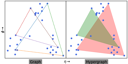
Figure 1: Visualisation of the inter-relations of jet constituents as captured by a graph structure (left) and a hypergraph structure with order-three hyperedges (right). In a graph structure, the edges correlate two constituents at a time and are shown as a line segment connecting two nodes. Instead, the order-three hyperedges simultaneously link properties of three jet constituents at a time and are shown as a triangle with vertices coinciding with three nodes. Thus, hypergraphs are more expressive structures and can access higher-order correlations amongst jet constituents.

With the recorded events naturally represented as sets (of variable sizes) of different reconstructed particles or raw detector hits, point clouds are the natural representation of the recorded data, and architectures to process such data efficiently, particularly Graph Neural Networks Qu:2019gqs ; Mikuni:2020wpr ; Bernreuther:2020vhm ; Blance:2020ktp ; Moreno:2019bmu ; Atkinson:2021nlt ; Atkinson:2021jnj ; Tsan:2021brw , have been used successfully for LHC phenomenology. However, graphs do not expose higher-order correlations within the data by design, concentrating on two-particle correlations–the natural generalisation being hypergraphs. This generalisation is diagrammatically shown in figure 1 for a three-prong top jet where the graph’s edges are defined in terms of two particles, while the order three hyperedges can look into the relevant three-prong structure of the top jet. This paper addresses these challenges by introducing Hypergraph Energy-weighted Message Passing Networks (H-EMPNs), which address some of the currently available infra-red and collinear (IRC) safe networks fail to address. We first examine the universal approximation capabilities of existing infra-red and collinear safe neural network models like Energy Flow Networks (EFNs) Komiske:2018cqr and Energy-weighted Message Passing Networks (EMPNs) Konar:2021zdg in approximating any IRC safe observable expressible in terms of C-correlators Tkachov:1995kk ; Komiske:2017aww looking into any general $N$-body phase space. Finding that EFNs are restricted $N=1$, and EMPNs have an arguably weak capability for approximating any $N\neq 2^{n}$ C-correlators, we present H-EMPN as a more robust and versatile model capable of efficiently approximating any general IRC safe observable for any general $N$. Our method leverages the power of message-passing in graphs and hypergraphs to capture higher-order relationships among the data points, thereby providing a more comprehensive feature extraction mechanism.

Restricting ourselves to $N=3$ for the top vs QCD jet tagging scenario, where the dominant information lies in the 3-body decay phase space of the top quark, we find that H-EMPNs outperform EMPN, which look up to $N=4$ interparticle correlations, confirming our initial observation. We demonstrate the efficacy of H-EMPNs through empirical tests to showcase the learned graph representations. Furthermore, we discuss the architectural nuances of H-EMPN, providing insights into its design and training procedures. By doing so, we aim to establish H-EMPN as a powerful tool for LHC phenomenology, opening new avenues for applications in collider phenomenology.

Specifically, in section 2, we discuss the universal approximation of any IRC safe observable by EFNs and EMPNs by taking its correspondence to any generic C-correlator. In section. 3, we devise H-EMPNs that can approximate any general C-correlator. The architecture and training details are presented in section 4, while the results are presented in section. 5. We conclude in section 6.

Notation

In the following discussions, we are given a set of massless particle four vectors

$$\mathcal{S}=\{\ p_{1},p_{2},....,p_{n_{part.}}\}\quad.$$

These particles will be indexed via small Roman subscripts, while the number of message-passing operations will be indexed as Greek superscripts. Unless otherwise stated, all summations will be over the set $\mathcal{S}$. The four vectors are given in terms of the relative hardness $z_{i}=p_{T}^{i}/\sum p_{T}^{j}$ and the rapidity-azimuth variables $\mathbf{\hat{p}}_{i}=(y_{i},\phi_{i})$. Bold-faced alphabets like $\mathbf{h}_{i}$ and $\mathbf{G}$ denote vector quantities with their italicized counterparts $h_{i}$ and $G$ acting as a placeholder for a component. As we will consider inference on networks after training rather than the training itself, we will not explicitly write the dependence of function approximators on the tunable parameters. For instance, $\mathbf{g}^{(\alpha)}(\mathbf{h}^{(\alpha-1)}_{i},\mathbf{h}^{(\alpha-1)}_{j})$ denote a MultiLayer Perceptron (MLP) at the $\alpha^{th}$ message passing step, $\mathbf{h}^{(\alpha-1)}_{i}$ and $\mathbf{h}^{(\alpha-1)}_{i}$ corresponds to the updated node features in the previous operation of particle $i$ and $j$, respectively, in $\mathcal{S}$.

2 Universal Approximation of IRC safe observables

In present scientific literature, it is well-known that MLPs are universal function approximators Cybenko1989 ; LESHNO1993861 ; arora2018understanding . Without going into mathematical rigour, a parametrized function $f(\mathbf{x},\Theta)$ of a vector $\mathbf{x}$ and tunable parameters $\Theta$, is a universal approximator if it can approximate any continuous function up to any arbitrary precision in a compact domain and range. On the other hand, physical observables like momenta or position live in an underlying metric space, and notions of completeness have long been the bread-and-butter of physicists to study physical systems. The complete set of IRC safe observables is essential at the LHC and the subject of our present investigation. Any IRC safe observable $\mathcal{O}$ can be expanded in a basis of C-correlators Tkachov:1995kk as

$$\mathcal{O}\approx\sum_{N=0}^{N_{max}}\;\mathcal{C}^{f_{N}}_{N}\quad,\quad\mathcal{C}^{f_{N}}_{N}=\sum_{i_{1}}\sum_{i_{2}}...\sum_{i_{N}}\,E_{i_{1}}E_{i_{2}}...E_{i_{N}}\,f_{N}(\hat{p}_{i_{1}},\hat{p}_{i_{2}},...\hat{p}_{i_{N}})\quad,$$ (1)

where $f_{N}$ is symmetric to any permutation of its arguments. Energy Flow Polynomials (EFPs) Komiske:2017aww expand $\mathcal{O}$ in a basis of polynomials in energy and separation $\Delta R_{ij}$ in the rapidity-azimuth plane using the Stone-Weistrass approximation theorem. In this section, we take a look into the approximation capabilities of existing IRC safe neural networks, namely Energy Flow Networks Komiske:2018cqr , and Energy-weighted Message Passing Network (EMPN) Konar:2021zdg , comparing the functional form to any arbitrary $N$ in the basis of C-correlators. As the C-correlators are complete, the network-extracted observables would be expressible as a linear sum of different C-correlators, and we investigate the terms in the sum (as given in eq. 1) that are optimally extracted via these observables.

Although we rely on the statement of universal approximation theorems, it is important to remember that we will strictly talk about the existence of such approximators and not concentrate on the method of finding such a function. However, presently available gradient descent algorithms are powerful enough to efficiently find an approximation given that we have the desired output value on a large enough number of samples. This numerical nature of finding a practical working point in the weight space is one of the significant concerns regarding the interpretability of neural networks in general. Our aim is not to tackle this more difficult problem but to systematically establish the capability of IRC-safe feature extractors based on their ability to approximate different C-correlators. Moreover, we concentrate on the extracted features rather than the final observable approximated by the complete network, i.e. we do not consider the function approximation done by the downstream MLP, which takes the extracted IRC safe features, as this would be akin to a usual multi-variate approach of physics motivated features.

As we will study the general behaviour of the approximated function whose weights are frozen after some training procedure, we will not discuss the explicit dependence of the neural networks on their tuneable parameters in the following discussions.

2.1 Energy Flow Networks

Energy Flow Networks are infra-red and collinear safe deep sets model which learns a per-particle map of each particle’s directional coordinates $\mathbf{\hat{p}}_{i}$ and undergoes an energy-weighted sum to form a fixed length representation of any variable cardinality constituent set. Without loss of generality for a multi-dimensional representation, a single IRC safe observable can be written as

$$C_{1}=\sum_{i}z_{i}\;g_{1}(\mathbf{\hat{p}}_{i})\quad,$$

where $g_{1}(\hat{p}_{i})$ represents a parameterised multilayer perceptron. We have specifically denoted the observable as $C_{1}$ to make it self-evident the per-particle map essentially approximates any general $\mathcal{C}_{1}^{f_{1}}$. This is because the MLP $g_{1}$ is a universal approximator and can approximate any function $f_{1}$ suiting a particular objective up to a required precision. In a practical implementation, several related IRC safe observables are approximated, which are fed to a downstream network for classification. The direct implementation of EFNs can, therefore, only extract features expressible in terms of $C_{1}$.

2.2 Energy-weighted Message Passing Networks

An energy-weighted message passing operation for any general parametrised function $\mathbf{\bar{g}}^{(\alpha)}$ can be written as

$$\mathbf{h}_{i}^{(\alpha+1)}=\sum_{j=\in\mathcal{N}[i]}\;\omega^{(\mathcal{N}[i])}_{j}\;\mathbf{\bar{g}}^{(\alpha+1)}(\mathbf{h}^{(\alpha)}_{i},\mathbf{h}^{(\alpha)}_{j})\quad,$$

where $\mathbf{h}^{(\alpha)}_{i}$ is the input node features for the $\alpha^{th}$ message passing operation and

$$\omega^{(\mathcal{N}[i])}_{j}=\frac{p_{T}^{j}}{\sum_{k=\in\mathcal{N}[i]}\;p^{k}_{T}}\quad$$

are the energy weights dependent on the IRC safe neighbourhood set $\mathcal{N}[i]$, with $\omega^{(S)}_{j}=z_{j}$, for the whole set $\mathcal{S}$. For notational convenience in the following discussions, we will take the sum over the full set of particles in the jet and replace $z_{j}$ in place of $\omega^{(\mathcal{N}[i])}_{j}$ without loss of generality. Therefore, we have

$$\mathbf{h}_{i}^{(\alpha+1)}=\sum_{j}\;z_{j}\;\mathbf{g}^{(\alpha+1)}(\mathbf{h}^{(\alpha)}_{i},\mathbf{h}^{(\alpha)}_{j})\quad$$ (2)

with the function $\mathbf{g}^{(\alpha+1)}$ expressed as a product of a Heaviside step functions $\Theta(\Delta R_{ij}<R_{0})$ and the original message function $\mathbf{\bar{g}}^{(\alpha+1)}$ as

$$\mathbf{g}^{(\alpha+1)}(\mathbf{h}^{(\alpha)}_{i},\mathbf{h}^{(\alpha)}_{j})=\Theta(\Delta R_{ij}<R_{0})\;\mathbf{\bar{g}}^{(\alpha+1)}(\mathbf{h}^{(\alpha)}_{i},\mathbf{h}^{(\alpha)}_{j})\quad.$$

Here, $\Delta R_{ij}$ is the Euclidean distance in the rapidity-azimuth plane between particle $i$ and $j$ while $R_{0}$ is the graph’s radius. The requirement of symmetry in the argument of $f_{2}(\mathbf{\hat{p}}_{i},\mathbf{\hat{p}}_{j})$ for $\mathcal{C}^{f_{2}}_{2}$ and its absence in eq. 2 is not a contradiction as the node features themselves are defined for each particle and hence are not IRC safe observables. In contrast, the IRC safe graph representation will generally be expressible as some linear combination of $\mathcal{C}_{N}$.

We have $\mathbf{h}^{(0)}_{i}=\mathbf{\hat{p}}_{i}$ which gives $\mathbf{\hat{p}}_{i}=\mathbf{\hat{p}}_{j}\implies\mathbf{h}^{(\alpha)}_{i}=\mathbf{h}^{(\alpha)}_{j}$ for any $\alpha>=0$ and any two collinear particles $i$ and $j$. The IRC safe graph representation is obtained as

$$\mathbf{G}^{(L)}=\sum_{i=1}^{i=N}\;z_{i}\;\mathbf{h}^{(L)}_{i}\quad,$$

after $L$ iterations. As we shall see in the following, the complexity of the extracted features via EMPN will depend on the value of $L$.

Explicitly for $L=1$, we have $\mathbf{h}_{i}^{(1)}=\sum_{j}z_{j}\;\mathbf{g}^{(1)}(\mathbf{\hat{p}}_{i},\mathbf{\hat{p}}_{j})$ which gives

$$\mathbf{G}^{(1)}=\sum_{i,j}\;z_{i}\;z_{j}\;\mathbf{g}^{(1)}(\mathbf{\hat{p}}_{i},\mathbf{\hat{p}}_{j})\quad.$$

If the symmetry is enforced in $\mathbf{g}^{(1)}$, the approximated observable will contain $\mathcal{C}_{2}^{f_{2}}$ term only. At the same time, a non-symmetric $\mathbf{g}^{(1)}$ would also have a $\mathcal{C}_{1}$ component.

For $L=2$, we have

$$\begin{split}\mathbf{G}^{(2)}&=\sum_{i,j}\;z_{i}\;z_{j}\;\mathbf{g}^{(2)}(\mathbf{h}^{(1)}_{i},\mathbf{h}^{(1)}_{j})\\ \implies\mathbf{G}^{(2)}&=\sum_{i,j}\;z_{i}\;z_{j}\;\mathbf{g}^{(2)}(\sum_{k}z_{k}\,\mathbf{g}^{(1)}(\mathbf{\hat{p}}_{i},\mathbf{\hat{p}}_{k}),\sum_{l}z_{l}\,\mathbf{g}^{(1)}(\mathbf{\hat{p}}_{j},\mathbf{\hat{p}}_{l}))~{}.\end{split}$$ (3)

The complicated nature of the arguments makes it difficult to ascertain the exact behaviour of the functional approximation. However, one expects the universal approximator $\mathbf{g}^{(2)}$ to be expressible as a linear combination of $\mathcal{C}_{N}$’s up to $N=4$. However, due to the presence of four angular arguments and four energy weights, it hints against the efficient approximation of any $\mathcal{C}_{N}^{f_{N}}$ for any $N<4$.

The situation is even more futile for $L=3$ with eight angular arguments and eight energy-weighted sums. For a particular $L$, we have $2^{L}$ angular arguments and the same number of energy-weighted sums. Even if one extracts the graph features at each stage $\alpha$, and gets a concatenated graph representation for each $\alpha>0$ up to $\alpha=L$, we have the efficient extraction of $2,2^{2},2^{3},....2^{L}$ terms the sum in eq. 1 for any general IRC safe observable $\mathcal{O}$. Although, for the jet substructure, one does not need to go to very high $N$, we already run into a problem for top-tagging, which has valuable information in the 3-prong structure of the energy deposits.

3 Hypergraph Energy-weighted Message Passing Networks

As discussed above, although powerful, Graph Neural Networks cannot look into higher-order relational information amongst the nodes efficiently. Therefore, in this section, we develop IRC-safe point cloud architectures capable of efficiently extracting higher-point correlation.

A possible way to extend the capabilities of IRC safe feature extraction to higher-point correlations is to directly implement the form of C-correlators as

$$\mathcal{H}^{N}=\sum_{i_{1}}\sum_{i_{2}}...\sum_{i_{N}}z_{i_{1}}z_{i_{2}}...z_{i_{N}}\;\Theta_{N}(\hat{p}_{i_{1}},\hat{p}_{i_{2}},...,\hat{p}_{i_{N}})\,\Phi_{N}(\hat{p}_{i_{1}},\hat{p}_{i_{2}},...,\hat{p}_{i_{N}})\quad,$$

where $\Theta_{N}$ are step functions for reducing the sums to localised information, and $\Phi_{N}$ are the neural networks approximating a correlated set (as the output of $\Phi_{N}$ in general, is a vector) of $f_{N}$’s for the particular training objective. For IRC safety, both $\Theta_{N}$ and $\Phi_{N}$ should be symmetric under the permutation of its arguments. The step function $\Theta_{N}$ for each $N$ essentially endows an $N$-uniform hypergraph structure onto the constituent set similar to the radius filter $\Theta(\Delta R_{ij}<R_{0})$ endowing a graph structure for the case of $\mathcal{C}_{2}$. Therefore, the concatenated hypergraph representations

$$\mathbf{X}=\oplus_{N}\mathcal{H}^{N}\quad,$$

up to $N_{max}$ would extract IRC safe features to be fed to a downstream MLP for some task.

We do not follow this approach for the following reasons. It is well-known 10.7551/mitpress/7496.003.0016 ; 10.1145/1390156.1390294 ; MAL-006 ; 7780459 that automatic feature extraction works best with deeper networks. Depth can only be brought into $\Phi_{N}$ in the above expression, which does nothing to the IRC-safe feature extraction process. The complexity can be increased by increasing $N$, which increases the width of the network, thereby increasing the model complexity sharply. Although the factorisation of the extracted features in energy and angular components could lead to better all-order behaviour in QCD and is indeed interesting, one needs to have proper control of the behaviour of the parameter optimisation before we can hope to answer such questions as demonstrated in ref Kasieczka:2020nyd .

Our approach is based on one-particle and two-particle messages to construct a hybrid message-passing neural network that can extract higher point correlations in a recursive approach. Although it is easily generalisable to higher-point information, we restrict ourselves up to 3-point interactions due to the increasing complexity.

3.1 IRC safety with heterogenous source and destination embeddings

The basic observation which makes it possible to build a higher-point IRC safe feature extractor is that the requirement of IRC safety for EMPN is still valid even when the node embedding for the source $\psi_{S}(\mathbf{\hat{p}}_{i})$, and destination $\psi_{D}(\mathbf{\hat{p}}_{i})$ are different as long as they separately satisfy

$$\psi_{S}(\mathbf{\hat{p}}_{q})=\psi_{S}(\mathbf{\hat{p}}_{r})=\psi_{S}(\mathbf{\hat{p}}_{s})\quad,\text{ and }\psi_{S}(\mathbf{\hat{p}}_{q})=\psi_{D}(\mathbf{\hat{p}}_{r})=\psi_{D}(\mathbf{\hat{p}}_{s})$$

when $\mathbf{\hat{p}}_{q}=\mathbf{\hat{p}}_{r}=\mathbf{\hat{p}}_{s}$, even if $\psi_{S}(\mathbf{\hat{p}}_{i})\neq\psi_{D}(\mathbf{\hat{p}}_{i})$. More importantly, the embeddings $\psi_{S}$ and $\psi_{D}$ need not be functions of just a single particle. They can also be the updated node features of the $\alpha$-hop IRC safe neighbourhood after $\alpha$ energy-weighted message passing operations (as given in eq. 2). For an IRC safe neighbourhood of $i$, where a particle $q$ splits to two daughters $r$ and $s$, we have $\mathcal{N}[i]\ni q\implies\mathcal{N}^{\prime}[i]\ni r\;\land\mathcal{N}^{\prime}[i]\ni s$ when $\mathbf{\hat{p}}_{q}=\mathbf{\hat{p}}_{r}=\mathbf{\hat{p}}_{s}$.

Let us look closer into the statement that we need not have the same embedding in the argument of the message function in an Energy-weighted Message Passing operation even though the statement logically follows from the non-requirement of symmetry of the message function. Since we have heterogeneous source and destination embeddings, we need to fix a uniform direction of messages. We will take all messages as originating from a neighbourhood node $j\in\mathcal{N}[i]$ and move towards the destination node $i$. Therefore, we have

$$\mathbf{H}_{i}^{(\alpha+1,\beta+1)}=\sum_{j}\;z_{j}\;\mathbf{g}^{(\alpha+1,\beta+1)}(\mathbf{h}^{(\alpha)}_{D,i},\mathbf{h}^{(\beta)}_{S,j})\quad,$$

where $\mathbf{h}^{(\alpha)}_{D,i}$ and $\mathbf{h}^{(\beta)}_{S,j}$ are the destination and source node embeddings, respectively, and $\mathbf{g}^{(\alpha+1,\beta+1)}$ is the corresponding message function. As the destination and source node embeddings differ, the message passing operations’ index is indexed separately with $\alpha$ and $\beta$, respectively. The source embedding satisfying $\mathbf{h}^{(\beta)}_{S,q}=\mathbf{h}^{(\beta)}_{S,r}=\mathbf{h}^{(\beta)}_{S,s}$ in the collinear limit makes the updated node representation $\mathbf{H}_{i}^{(\alpha+1,\beta+1)}$ equal for $i\notin\{q,r,s\}$, in the splitted and unsplitted case since $z_{q}=z_{r}+z_{s}$. Explicitly, we have

$$z_{q}\;\mathbf{g}^{(\alpha+1,\beta+1)}(\mathbf{h}^{(\alpha)}_{D,i},\mathbf{h}^{(\beta)}_{S,q})=z_{r}\;\mathbf{g}^{(\alpha+1,\beta+1)}(\mathbf{h}^{(\alpha)}_{D,i},\mathbf{h}^{(\beta)}_{S,r})+z_{s}\;\mathbf{g}^{(\alpha+1,\beta+1)}(\mathbf{h}^{(\alpha)}_{D,i},\mathbf{h}^{(\beta)}_{S,s})\quad.$$ (4)

Additionally, we require the equality of the destination embeddings $\mathbf{h}^{(\alpha)}_{D,q}=\mathbf{h}^{(\alpha)}_{D,r}=\mathbf{h}^{(\alpha)}_{D,s}$ when $i\in\{q,r,s\}$. However, we can have $\mathbf{h}^{(\alpha)}_{D,q}\neq\mathbf{h}^{(\beta)}_{S,q}$, as this is not needed to satisfy eq. 4. Therefore, $\mathbf{H}^{(\alpha+1,\beta+1)}_{i}$ satisfies $\mathbf{H}^{(\alpha+1,\beta+1)}_{q}=\mathbf{H}^{(\alpha+1,\beta+1)}_{r}=\mathbf{H}^{(\alpha+1,\beta+1)}_{s}$, in the collinear limit of the two daughters $r$ and $s$ of $q$.

3.2 Building higher point IRC safe feature extractor

It is now straightforward to build an IRC-safe message-passing operation which looks into three-particle correlations. The structure of the two-particle energy-weighted operation is kept the same as rq. 2, and then combined with destination embedding $\psi_{D}(\mathbf{\hat{p}}_{i})$ and source embedding $\psi_{R}(\mathbf{\hat{p}}_{i})$ of the angular coordinates to give an effective three particle message passing of the form

$$\begin{split}\mathbf{H}^{(1,2)}_{i}&=\sum_{j}\;z_{j}\;\mathbf{g}^{(1,2)}(\psi_{D}(\mathbf{\hat{p}}_{i}),\mathbf{h}^{(1)}_{S,j})\quad,\\ \mathbf{H}^{(2,1)}_{i}&=\sum_{j}\;z_{j}\;\mathbf{g}^{(2,1)}(\mathbf{h}^{(1)}_{D,i},\psi_{S}(\mathbf{\hat{p}}_{j}))\quad.\end{split}$$ (5)

As the destination and source embeddings are different, $\mathbf{h}^{(1)}_{D,i}$ and $\mathbf{h}^{(1)}_{S,i}$ denote node features updated after two separate message-passing operations as given in eq. 2 with different message functions $\mathbf{g}^{(1)}_{D}$ and $\mathbf{g}^{(1)}_{S}$, respectively. The IRC safe feature would be a graph-level representation after an energy-weighted summed graph readout on $\mathbf{H}^{(1,2)}_{i}$ and $\mathbf{H}^{(2,1)}_{i}$, as

$$\mathbf{G}^{(1,2)}_{3}=\sum_{i}\;z_{i}\;\mathbf{H}^{(1,2)}_{i}\quad,\quad\mathbf{G}^{(2,1)}_{3}=\sum_{i}\;z_{i}\;\mathbf{H}^{(2,1)}_{i}\quad.$$ (6)

We shall see in the following discussions that these two representations look at distinct topological structures in the graph; the IRC safe representation for the order three feature extraction is constructed as a concatenation of these two components

$$\mathbf{G}_{3}=\mathbf{G}^{(1,2)}_{3}\oplus\mathbf{G}^{(2,1)}_{3}\quad.$$

We can ascertain the behaviour of $\mathbf{G}_{3}$ by writing down its dependence on the particle’s four vectors:

$$\begin{split}\mathbf{G}_{3}&=\sum_{i,j}\;z_{i}\,z_{j}\;\left(\mathbf{g}^{(1,2)}(\psi_{D}(\mathbf{\hat{p}}_{i}),\sum_{l}\;z_{l}\,\mathbf{g}^{(1)}_{S}(\mathbf{\hat{p}}_{j},\mathbf{\hat{p}}_{l}))\right.\\ &\quad\quad\quad\quad\quad\quad\oplus\left.\mathbf{g}^{(2,1)}(\sum_{l}\,z_{l}\,\mathbf{g}^{(1)}_{D}(\mathbf{\hat{p}}_{i},\mathbf{\hat{p}}_{l}),\psi_{S}(\mathbf{\hat{p}}_{j})\right)\quad.\end{split}$$

Three energy weights and three angular arguments hint that the learning procedure would directly start looking at the three-particle interrelations. It is important to note that any IRC safe observable looking into $n$ body phase space, by definition, approaches its $n-1$ body phase space limit when one particle approaches the soft or collinear limit. In other words, eq. 3 will also look into the three-body limit of any four-particle combination when one is soft or collinear to any other particle. However, we expect the above form to extract better the three-particle correlations required for tagging three-prong jets like top quarks.

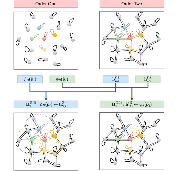
Figure 2: The figure shows a schematic representation of the message passing operation to build hybrid order three node representations for Hypergraph Energy-weighted Message Passing Networks by combining order one and two node representations.

A schematic representation of the feature extraction procedure using different source and destination embeddings of order one and order two operations is shown in figure 2. We focus on the red node whose neighbours are the coloured. On the top right, the per-particle embeddings for the source and destination can only look into the individual particle information. On the left, however, the energy-weighted message-passing operation gathers information from each node’s neighbourhood, which are shown with the identically coloured arrows for the coloured nodes. The order three feature extractors are built by combining the per-particle destination embedding with the order-two source embedding (on the left) and the order-two destination embedding with the per-particle source embedding (on the right).

From a feature extraction perspective, there are two essential differences in comparison to the $L=2$ case given in eq. 3:

• One argument in both $\mathbf{g}^{(1,2)}$ and $\mathbf{g}^{(2,1)}$ is an embedding of the angular coordinates of a single particle and hence contain single-particle information. In contrast, both arguments already contain the aggregated neighbourhood information in $\mathbf{g}^{(2)}$.

• The embedding of the two arguments in $\mathbf{g}^{(1,2)}$ and $\mathbf{g}^{(2,1)}$ have independently trainable weights while they are shared for $\mathbf{g}^{(2)}$.

The first difference makes it possible for the function $\mathbf{g}^{(1,2)}$ to effectively extract the relation of each node $i$ concerning the IRC safe 2-hop neighbourhood, while the function $\mathbf{g}^{(2,1)}$ looks at the aggregated node feature of $i$’s immediate neighbourhood with individual nodes in the same neighbourhood. The difference is also seen in figure 2, where on the left $\mathbf{H}^{(1,2)}_{i}$ looks into the features of the nodes within each coloured circle with the red node, while on the right, $\mathbf{H}^{(2,1)}_{i}$ looks into the feature of the aggregated neighbourhood information of the red node with the individual nodes within its neighbourhood. This essential difference in the feature extraction procedure makes it imperative to devise the two separate message-passing operations as they need to extract topologically different features within the graph.

It is straightforward to generalize this procedure to any arbitrary $N$, with substantial flexibility to choose the extractor guided by the requirement to divide $N$ into two parts in any possible way. Any feature extractor with $N-1$ can be used to extract features from topological distinct paths of length $N$ within the graph. Due to the different combinatorial factors involved, the complexity rises relatively fast with increasing $N$, and we restrict our discussion to $N=3$.

To look into the learnt features of the order one and two feature extractors, we define the graph representation as a concatenation of the source and destination embeddings as

$$\begin{split}\mathbf{G}_{1}&=\mathbf{G}_{D,1}\oplus\mathbf{G}_{S,1}=\sum_{i}\;z_{i}\;(\psi_{D}(\mathbf{\hat{p}}_{i})\oplus\psi_{S}(\mathbf{\hat{p}}_{i}))\quad,\\ \mathbf{G}_{2}&=\mathbf{G}_{D,2}\oplus\mathbf{G}_{S,2}=\sum_{i}\;z_{i}\;(\mathbf{h}^{(1)}_{D,i}\oplus\mathbf{h}^{(1)}_{S,i})\quad.\end{split}$$ (7)

This gives the concatenated graph readout to be fed to the classifier network as

$$\mathbf{G}=\mathbf{G}_{1}\oplus\mathbf{G}_{2}\oplus\mathbf{G}_{3}\quad.$$ (8)

4 Network architecture and training

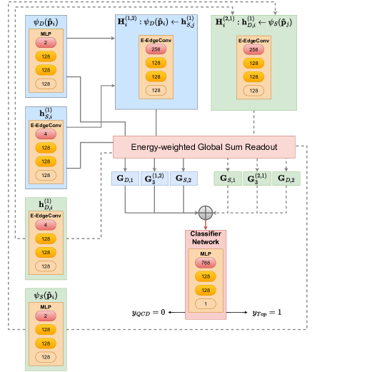
Figure 3: The architecture of the H-EMPN network utilized in this study is shown in the figure above.

To gauge the properties of the proposed network, we utilise the public top-tagging dataset kasieczka_gregor_2019_2603256 for a supervised classifier. These events were generated with Pythia 8.2.15 Sjostrand:2014zea and were showered and hadronised without MPI effects. The showered events additionally underwent a parametrised detector response via Delphes3 deFavereau:2013fsa with the default ATLAS detector card. The particle-flow objects of the Delphes output were used as inputs to construct anti-$k_{T}$ Cacciari:2008gp jets with $R=0.8$ via FastJet Cacciari:2011ma . with additional requirements of $p_{T}$ within the range $[550,650]$ GeV, and pseudorapidity $|\eta|<2$. Further, for the signal events, the top quark and its decay products’ parton level information were used to reject falsely reconstructed jets with the partons falling outside the jet’s area. The training data comprises 1.2 million samples, while the test and validation datasets contain 400k samples. The network analysis uses PyTorch-Geometric  Fey/Lenssen/2019 .

We compare order three Hypergraph Energy-weighted Message Passing Networks (H-EMPNs) with $L=2$ EMPNs. For a reasonable comparison with the H-EMPN, we will extract the graph features for $\alpha=1$ and $\alpha=2$ stages separately for the EMPN and feed the concatenated graph representation into the classifier network. As shown in figure 3, the IRC-safe feature extractor module for the H-EMPN, in total, contains two per-particle maps for $\psi_{D}$ and $\psi_{S}$, and four energy-weighted edge convolution (E-EdgeConv) operations to give the updated node embeddings $\mathbf{h}^{(1)}_{D,i}$, $\mathbf{h}^{(1)}_{S,i}$, $\mathbf{H}^{(1,2)}_{i}$, and $\mathbf{H}^{(2,1)}_{i}$. Including the classifier MLP, which takes in the concatenated graph readout, we have seven MLPs. We have one for each per-particle map and a message function for each E-EdgeConv operation from the feature extractor module. All these seven MLPs contain two hidden layers with 128 nodes and a rectified linear unit activation function. Except for the classifier network, which has a one-dimensional output with sigmoid activation, all other MLPs have a 128-dimensional output layer with a linear activation function. The per-particle maps take the rapidity-azimuth coordinates $\mathbf{\hat{p}}_{i}=(\Delta y_{iJ},\Delta\phi_{iJ})$ of each constituent $i$ as inputs with the differences taken from the jet axis defined by the four-vector $p^{\mu}_{J}=\sum_{k\in\mathcal{S}}p^{k}_{\mu}$. For a destination node embedding $\mathbf{h}_{S,i}$ and source node embedding $\mathbf{h}_{D,i}$, the message function takes in the concatenated vector $\mathbf{h}_{S,i}\oplus\mathbf{h}_{S,i}-\mathbf{h}_{S,j}$ as the input. The EMPN network sequentially applies the E-EdgeConv operation twice to the input graph’s node features. The first and the second E-EdgeConv operations have the same MLP architecture corresponding to the ones that give $\mathbf{h}^{(1)}_{D,i}/\mathbf{h}^{(1)}_{D,i}$ and $\mathbf{H}^{(1,2)}_{i}/\mathbf{H}^{(2,1)}_{i}$, respectively. The classifier MLP for the EMPN and H-EMPN takes in 256 and 768-dimensional concatenated graph representations, respectively. The whole network is trained using the binary-cross entropy loss function.

We construct graphs with $R_{0}\in\{0.4,0.5,0.6\}$ and $R_{0}\to\infty$ corresponding to complete graphs. For all these four instances of input graphs, we train each network five times from random initialization for 100 epochs with the Adam optimizer DBLP:journals/corr/KingmaB14 and a learning rate of 0.001. A decay-on-plateau condition is applied to the learning rate with a decay factor of 0.5 if the validation loss does not decrease for three epochs. The epoch with minimum validation loss is used for inference for each training instance.

5 Results

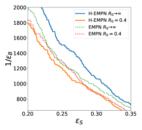
Figure 4: The receiver operator characteristics curve for the best performing network (in terms of AUC) over the five training instances for $R_{0}=0.4$ and $R_{0}\to\infty$ for the EMPN and H-EMPN for different ranges of signal acceptance $\epsilon_{S}$.

5.1 Performance

The receiver operator characteristics (ROC) curve for the network with highest area under the ROC (AUC) curve from all training instances between the signal acceptance $\epsilon_{S}$ and the inverse of background acceptance $1/\epsilon_{B}$ for the two models for $R_{0}=0.4$ and $R_{0}\to\infty$ is shown in figure 4. We see that the EMPN has almost an overlapping ROC curve for these two radii, while for the H-EMPN, there is a noticeable improvement. The area under the receiver operator curve for the EMPN and H-EMPN and different graph construction radii are tabulated in table 1. The values correspond to the mean over the five training instances, while the errors correspond to the standard deviation. For $R_{0}=0.4$, the EMPN and H-EMPN have almost identical discrimination power with an AUC of 0.9823 and 0.9821, respectively. As the radius increases, there is a steady increase for the H-EMPN, while for the EMPN, it increases for $R_{0}=0.5$ and stays at a similar value for $R_{0}=0.6$ and there is a noticeable dip in performance when going to complete graphs with $R_{0}\to\infty$. This trend can be understood from the structural difference between the EMPN and H-EMPN. The EMPN’s feature extraction is sequential, with the second E-EdgeConv being fed by the first E-EdgeConv’s updated node features. With increasing radius, the feature extraction suffers from a redundancy of the information as the first E-EdgeConv already looks at a much larger neighbourhood in the rapidity-azimuth plane. On the other hand, the H-EMPN has a much larger width, with four modules taking the input jet constituents parallelly, which are then combined non-trivially to feed the order-three feature extractors. From a purely QCD perspective, the radius $R_{0}$ puts in an additional scale, and going to the $R_{0}\to\infty$ limit takes away this dependence in the feature extraction procedure. Therefore, the H-EMPN can extract features from the full jet more efficiently without being restrained by an arbitrary angular scale $R_{0}$.

The AUC paints a global picture of the discrimination power of a binary classifier; however, a classifier is almost always used at a specific working point, depending on the analysis. This practical aspect demands a local figure of merit, which we show with the inverse of the background acceptance $\epsilon_{B}$, the background rejection $1/\epsilon_{B}$, at fixed values of signal acceptance $\epsilon_{S}$. The background rejection for the EMPN and H-EMPN for the different graph construction radii are shown for $\epsilon_{S}=0.5$ and $\epsilon_{S}=0.3$ in tables 2 and 3, respectively. The values are averaged over the five training instances, with the standard deviations shown as errors. Although the trend for separate models is similar to that of the AUCs, the H-EMPN already starts having a noticeably better background rejection for $R_{0}=0.5$ even though the EMPN has a nominally higher AUC. As a matter of fact, except for $R_{0}=0.4$ at $\epsilon_{S}=0.3$, the H-EMPN has a numerically higher mean background rejection for all other instances.

	Area Under the ROC Curve
Model	$R_{0}=0.4$	$R_{0}=0.5$	$R_{0}=0.6$	$R_{0}\to\infty$
EMPN	$0.9823\pm 0.00015$	$0.9827\pm 0.00009$	$0.9826\pm 0.00024$	$0.9825\pm 0.00015$
H-EMPN	$0.9821\pm 0.00012$	$0.9826\pm 0.00010$	$0.9828\pm 0.00029$	$0.9834\pm 0.00012$

Table 1: The table shows the mean AUC for five training instances evaluated on the test dataset of the public top-tagging dataset for different architectures. The errors shown are the standard deviation of the five training instances.

	$1/\epsilon_{B}$ at $\epsilon_{S}=0.5$
Model	$R_{0}=0.4$	$R_{0}=0.5$	$R_{0}=0.6$	$R_{0}\to\infty$
EMPN	$235\pm 7$	$250\pm 2$	$246\pm 4$	$255\pm 6$
H-EMPN	$236\pm 2$	$258\pm 6$	$258\pm 11$	$276\pm 6$

Table 2: The table shows the background rejection at a signal acceptance of 50% for different models. The values correspond to the mean from the evaluation of the test dataset for five different training instances from random initialization, while the standard deviations are shown as errors.

	$1/\epsilon_{B}$ at $\epsilon_{S}=0.3$
Model	$R_{0}=0.4$	$R_{0}=0.5$	$R_{0}=0.6$	$R_{0}\to\infty$
EMPN	$819\pm 39$	$882\pm 11$	$839\pm 31$	$895\pm 36$
H-EMPN	$817\pm 33$	$917\pm 25$	$911\pm 34$	$995\pm 48$

Table 3: The table shows the background rejection ($1/\epsilon_{B})$ at a signal acceptance ($\epsilon_{S}$) of 30% for different models. The values correspond to the mean from the evaluation of the test dataset for five different training instances from random initialization, while the standard deviations are shown as errors.

5.2 Visualizing the latent graph representation

Figure 5: The two-dimensional histogram of the QCD (above) and top (below) test datasets in the two-dimensional latent space obtained after a t-SNE embedding of the 128-dimensional graph representation $\mathbf{G}^{(1)}$ (left) and $\mathbf{G}^{(2)}$ (right) of the best performing EMPN trained with complete graphs.

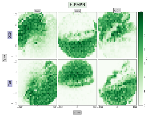
Figure 6: The two-dimensional histogram of the QCD (above) and top (below) test datasets in the two-dimensional latent space obtained after a t-SNE embedding of the 128-dimensional graph representation $\mathbf{G}_{D,1}$ (left), $\mathbf{G}_{D,2}$ (center) and $\mathbf{G}^{(1,2)}_{3}$ (right) of the best performing H-EMPN trained with complete graphs.

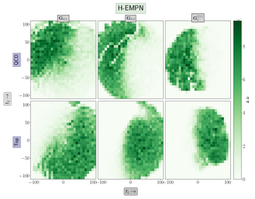
Figure 7: The two-dimensional histogram of the QCD (above) and top (below) test datasets in the two-dimensional latent space obtained after a t-SNE embedding of the 128-dimensional graph representation $\mathbf{G}_{S,1}$ (left), $\mathbf{G}_{S,2}$ (center) and $\mathbf{G}^{(2,1)}_{3}$ (right) of the best performing H-EMPN trained with complete graphs.

In this section, we investigate whether all the graph representations that the H-EMPN learns can contribute to separating the signal and the background for the final classifier output. We choose the best-performing complete graph, which has the possibility of the highest information redundancy besides being the strongest classifier. Although a relatively high linear correlation with the network output does point to the classification using that particular information, it is defined for each component of the graph representation, which dilutes the importance of the underlying vector representations. Moreover, the absence of linear correlation does not imply the lack of discriminatory information, as neural networks can be highly non-linear functions of their inputs.

We look into the separating power of the different graph representations by visualizing them in a two-dimensional latent space using the t-distributed Stochastic Neighbourhood Embedding (t-SNE) JMLR:v9:vandermaaten08a —an unsupervised data representation technique, where high dimensional data is embedded non-linearly in a lower dimensional space by maximally conserving the neighbourhood information endowed by a Euclidean metric in both spaces. In other words, nearby points in the high-dimensional representation get mapped to a local neighbourhood in the low-dimensional space. As it is an unsupervised technique, no explicit class information (QCD and top for our case) is fed when learning the map, and the clusters that arise in the low-dimensional space are a consequence of their proximity in the high-dimensional space. Therefore, a well-separated cluster in the lower-dimensional space implies that the higher-dimensional space also has well-separated regions.

We use the implementation of t-SNE in Scikit-learn scikit-learn package to embed the various 128-dimensional graph representations of the test dataset evaluated on the best performing EMPN and H-EMPN for the complete graph in a two-dimensional space separately for each representation. The class-wise two-dimensional histogram in the embedding space $(t_{1},t_{2})$ for $\mathbf{G}^{(1)}$ and $\mathbf{G}^{(2)}$ for the EMPN are shown in figure 5. We can see that both the graph representations have relatively distinct regions in $(t_{1},t_{2})$ for the QCD samples (shown above) and top samples (shown below). Similarly, the two-dimensional histograms for the graph representations constructed out of the destination and source node-embeddings for the H-EMPN are shown in figures 6 and 7, respectively. All these embedded graph representations exhibit clear clustering of the QCD and top samples in different regions, confirming that the H-EMPN has extracted discriminating features from all of its component modules.

Although the EMPN and H-EMPN can utilize their constituent graph representation to separate the QCD jets from top jets as seen from these two-dimensional histograms, we reiterate the qualitative differences between these two networks from the QCD perspective. The $L=2$ EMPN looks up to order four relations. In contrast, the H-EMPN in its present guise only looks up to order three–the sequential application of E-EdgeConv (to give $\mathbf{H}^{(1,2)}_{i}$ and $\mathbf{H}^{(2,1)}_{i}$) takes in the per-particle map with single particle information rather than an updated node feature with the local neighbourhood information in one of its arguments. However, we can see the better ability of the H-EMPN network from its performance studies and potentially better behaviour in QCD with its greater efficacy in the absence of an arbitrary angular scale $R_{0}$. Since we took the top vs QCD jets classification example, we already knew that there is beneficial information in the three-prong structure within the jet, which prompted our design of the specific H-EMPN. The first observation from the finite $R_{0}$ cases is that the H-EMPN architecture is more critical in extracting the order three relational information from the jets than the $L=2$ EMPN. On the other hand, our a priori knowledge of QCD, prompting the design of the H-EMPN, validates that physical inductive biases, or more specifically, QCD, have an important role in the design of performant feature extractors. Therefore, rather than throwing a currently “fashionable network” under the hood, designing architectures based on the underlying physical intuition can help push the performance boundaries of deep learning algorithms and gain (at least) a qualitative understanding of their inner workings.

6 Conclusions

This study delved deep into the intricacies of generalised automatic infrared and collinear safe feature extraction for LHC phenomenology, focusing on the potential of Graphs and Hypergraphs. Hypergraphs are a generalisation of traditional graphs. While a standard graph consists of vertices connected by edges, each connecting exactly two vertices, a hypergraph allows edges to connect any number of vertices, offering a more flexible way to represent relationships between entities.

First, we explored the behaviour of energy-weighted message passing and its capability to approximate general infrared and collinear safe observables. We highlighted the significance of IRC-safe observables, especially in the context of data interpretation at LHC experiments. The study further explored the capabilities of Energy Flow Networks and Energy-weighted message-passing networks, shedding light on their potential and constraints utilising the usage of multilayer perceptrons as universal function approximators within the architecture with the IRC-safe observables expressible in terms of C-correlators.

To enhance the capabilities of IRC safe feature extraction, especially for higher-point correlations, a novel method was introduced by leveraging the form of C-correlators and heterogenous source and destination node embeddings. This approach presents a renewed outlook on feature extraction.

Qualitatively assessing the two models, while the EMPN model provides a robust foundation for feature extraction, the H-EMPN model, designed to look at order-three interparticle relations, demonstrates an edge in performance metrics even though the EMPN model via the application of two-message passing operations could theoretically look up to order-four. This suggests that incorporating hypergraph structures in the H-EMPN model offers enhanced capabilities in extracting higher-point correlations, making it a promising tool for more intricate analyses in LHC phenomenology.

Our findings underscore the potential of hypergraph-based methods in enhancing the extraction of IRC-safe features. The research paves the way for further exploration into LHC phenomenology, focusing on optimising feature extraction techniques.

References

- (1) A. Andreassen, P. T. Komiske, E. M. Metodiev, B. Nachman and J. Thaler, OmniFold: A Method to Simultaneously Unfold All Observables, Phys. Rev. Lett. 124 (2020) 182001 [1911.09107].
- (2) P. T. Komiske, E. M. Metodiev and J. Thaler, Metric Space of Collider Events, Phys. Rev. Lett. 123 (2019) 041801 [1902.02346].
- (3) S. Bieringer, A. Butter, T. Heimel, S. Höche, U. Köthe, T. Plehn et al., Measuring QCD Splittings with Invertible Networks, SciPost Phys. 10 (2021) 126 [2012.09873].
- (4) D. Kim, K. Kong, K. T. Matchev, M. Park and P. Shyamsundar, Deep-learned event variables for collider phenomenology, Phys. Rev. D 107 (2023) L031904 [2105.10126].
- (5) Y. S. Lai, J. Mulligan, M. Płoskoń and F. Ringer, The information content of jet quenching and machine learning assisted observable design, JHEP 10 (2022) 011 [2111.14589].
- (6) A. Romero, D. Whiteson, M. Fenton, J. Collado and P. Baldi, Safety of Quark/Gluon Jet Classification, 2103.09103.
- (7) J. Batson, C. G. Haaf, Y. Kahn and D. A. Roberts, Topological Obstructions to Autoencoding, JHEP 04 (2021) 280 [2102.08380].
- (8) I. Chahrour and J. D. Wells, Comparing machine learning and interpolation methods for loop-level calculations, SciPost Phys. 12 (2022) 187 [2111.14788].
- (9) A. Butter, B. M. Dillon, T. Plehn and L. Vogel, Performance versus Resilience in Modern Quark-Gluon Tagging, 2212.10493.
- (10) F. A. Dreyer, R. Grabarczyk and P. F. Monni, Leveraging universality of jet taggers through transfer learning, Eur. Phys. J. C 82 (2022) 564 [2203.06210].
- (11) P. Onyisi, D. Shen and J. Thaler, Comparing point cloud strategies for collider event classification, Phys. Rev. D 108 (2023) 012001 [2212.10659].
- (12) Z. Kassabov, M. Madigan, L. Mantani, J. Moore, M. Morales Alvarado, J. Rojo et al., The top quark legacy of the LHC Run II for PDF and SMEFT analyses, JHEP 05 (2023) 205 [2303.06159].
- (13) A. Butter, N. Huetsch, S. P. Schweitzer, T. Plehn, P. Sorrenson and J. Spinner, Jet Diffusion versus JetGPT – Modern Networks for the LHC, 2305.10475.
- (14) W. Shen, D. Wang and J. M. Yang, Hierarchical High-Point Energy Flow Network for Jet Tagging, 2308.08300.
- (15) A. Rousselot and M. Spannowsky, Generative Invertible Quantum Neural Networks, 2302.12906.
- (16) A. Andreassen, I. Feige, C. Frye and M. D. Schwartz, JUNIPR: a Framework for Unsupervised Machine Learning in Particle Physics, Eur. Phys. J. C 79 (2019) 102 [1804.09720].
- (17) S. Choi, S. J. Lee and M. Perelstein, Infrared Safety of a Neural-Net Top Tagging Algorithm, JHEP 02 (2019) 132 [1806.01263].
- (18) F. A. Dreyer and H. Qu, Jet tagging in the Lund plane with graph networks, JHEP 03 (2021) 052 [2012.08526].
- (19) T. Faucett, J. Thaler and D. Whiteson, Mapping Machine-Learned Physics into a Human-Readable Space, Phys. Rev. D 103 (2021) 036020 [2010.11998].
- (20) Y. S. Lai, D. Neill, M. Płoskoń and F. Ringer, Explainable machine learning of the underlying physics of high-energy particle collisions, Phys. Lett. B 829 (2022) 137055 [2012.06582].
- (21) A. Bogatskiy, T. Hoffman, D. W. Miller, J. T. Offermann and X. Liu, Explainable Equivariant Neural Networks for Particle Physics: PELICAN, 2307.16506.
- (22) D. Athanasakos, A. J. Larkoski, J. Mulligan, M. Płoskoń and F. Ringer, Is infrared-collinear safe information all you need for jet classification?, 2305.08979.
- (23) S. Bollweg, M. Haußmann, G. Kasieczka, M. Luchmann, T. Plehn and J. Thompson, Deep-Learning Jets with Uncertainties and More, SciPost Phys. 8 (2020) 006 [1904.10004].
- (24) A. Ghosh, B. Nachman and D. Whiteson, Uncertainty-aware machine learning for high energy physics, Phys. Rev. D 104 (2021) 056026 [2105.08742].
- (25) R. Gambhir, B. Nachman and J. Thaler, Learning Uncertainties the Frequentist Way: Calibration and Correlation in High Energy Physics, Phys. Rev. Lett. 129 (2022) 082001 [2205.03413].
- (26) A. Butter, T. Heimel, S. Hummerich, T. Krebs, T. Plehn, A. Rousselot et al., Generative networks for precision enthusiasts, SciPost Phys. 14 (2023) 078 [2110.13632].
- (27) R. T. d’Agnolo, G. Grosso, M. Pierini, A. Wulzer and M. Zanetti, Learning new physics from an imperfect machine, Eur. Phys. J. C 82 (2022) 275 [2111.13633].
- (28) M. Bellagente, M. Haussmann, M. Luchmann and T. Plehn, Understanding Event-Generation Networks via Uncertainties, SciPost Phys. 13 (2022) 003 [2104.04543].
- (29) A. Ghosh and B. Nachman, A cautionary tale of decorrelating theory uncertainties, Eur. Phys. J. C 82 (2022) 46 [2109.08159].
- (30) A. Ghosh, B. Nachman, T. Plehn, L. Shire, T. M. P. Tait and D. Whiteson, Statistical patterns of theory uncertainties, SciPost Phys. Core 6 (2023) 045 [2210.15167].
- (31) P. T. Komiske, E. M. Metodiev and J. Thaler, Energy Flow Networks: Deep Sets for Particle Jets, JHEP 01 (2019) 121 [1810.05165].
- (32) A. Bogatskiy, B. Anderson, J. T. Offermann, M. Roussi, D. W. Miller and R. Kondor, Lorentz Group Equivariant Neural Network for Particle Physics, 2006.04780.
- (33) G. Kasieczka, S. Marzani, G. Soyez and G. Stagnitto, Towards Machine Learning Analytics for Jet Substructure, JHEP 09 (2020) 195 [2007.04319].
- (34) S. Badger and J. Bullock, Using neural networks for efficient evaluation of high multiplicity scattering amplitudes, JHEP 06 (2020) 114 [2002.07516].
- (35) D. Maître and H. Truong, A factorisation-aware Matrix element emulator, JHEP 11 (2021) 066 [2107.06625].
- (36) P. Konar, V. S. Ngairangbam and M. Spannowsky, Energy-weighted message passing: an infra-red and collinear safe graph neural network algorithm, JHEP 02 (2022) 060 [2109.14636].
- (37) S. Gong, Q. Meng, J. Zhang, H. Qu, C. Li, S. Qian et al., An efficient Lorentz equivariant graph neural network for jet tagging, JHEP 07 (2022) 030 [2201.08187].
- (38) Z. Hao, R. Kansal, J. Duarte and N. Chernyavskaya, Lorentz group equivariant autoencoders, Eur. Phys. J. C 83 (2023) 485 [2212.07347].
- (39) S. E. Park, P. Harris and B. Ostdiek, Neural embedding: learning the embedding of the manifold of physics data, JHEP 07 (2023) 108 [2208.05484].
- (40) O. Atkinson, A. Bhardwaj, C. Englert, P. Konar, V. S. Ngairangbam and M. Spannowsky, IRC-Safe Graph Autoencoder for Unsupervised Anomaly Detection, Front. Artif. Intell. 5 (2022) 943135 [2204.12231].
- (41) H. Qu and L. Gouskos, ParticleNet: Jet Tagging via Particle Clouds, Phys. Rev. D 101 (2020) 056019 [1902.08570].
- (42) V. Mikuni and F. Canelli, ABCNet: An attention-based method for particle tagging, Eur. Phys. J. Plus 135 (2020) 463 [2001.05311].
- (43) E. Bernreuther, T. Finke, F. Kahlhoefer, M. Krämer and A. Mück, Casting a graph net to catch dark showers, SciPost Phys. 10 (2021) 046 [2006.08639].
- (44) A. Blance and M. Spannowsky, Unsupervised event classification with graphs on classical and photonic quantum computers, JHEP 21 (2020) 170 [2103.03897].
- (45) E. A. Moreno, O. Cerri, J. M. Duarte, H. B. Newman, T. Q. Nguyen, A. Periwal et al., JEDI-net: a jet identification algorithm based on interaction networks, Eur. Phys. J. C 80 (2020) 58 [1908.05318].
- (46) O. Atkinson, A. Bhardwaj, C. Englert, V. S. Ngairangbam and M. Spannowsky, Anomaly detection with convolutional Graph Neural Networks, JHEP 08 (2021) 080 [2105.07988].
- (47) O. Atkinson, A. Bhardwaj, S. Brown, C. Englert, D. J. Miller and P. Stylianou, Improved constraints on effective top quark interactions using edge convolution networks, JHEP 04 (2022) 137 [2111.01838].
- (48) S. Tsan, R. Kansal, A. Aportela, D. Diaz, J. Duarte, S. Krishna et al., Particle Graph Autoencoders and Differentiable, Learned Energy Mover’s Distance, in 35th Conference on Neural Information Processing Systems, 11, 2021, 2111.12849.
- (49) F. V. Tkachov, Measuring multi - jet structure of hadronic energy flow or What is a jet?, Int. J. Mod. Phys. A 12 (1997) 5411 [hep-ph/9601308].
- (50) P. T. Komiske, E. M. Metodiev and J. Thaler, Energy flow polynomials: A complete linear basis for jet substructure, JHEP 04 (2018) 013 [1712.07124].
- (51) G. Cybenko, Approximation by superpositions of a sigmoidal function, Mathematics of Control, Signals and Systems 2 (1989) 303.
- (52) M. Leshno, V. Y. Lin, A. Pinkus and S. Schocken, Multilayer feedforward networks with a nonpolynomial activation function can approximate any function, Neural Networks 6 (1993) 861.
- (53) R. Arora, A. Basu, P. Mianjy and A. Mukherjee, Understanding deep neural networks with rectified linear units, in International Conference on Learning Representations, 2018.
- (54) Y. Bengio and Y. LeCun, Scaling Learning Algorithms toward AI, in Large-Scale Kernel Machines, The MIT Press, (08, 2007), https://direct.mit.edu/book/chapter-pdf/2141379/9780262255790_can.pdf, DOI.
- (55) P. Vincent, H. Larochelle, Y. Bengio and P.-A. Manzagol, Extracting and composing robust features with denoising autoencoders, in Proceedings of the 25th International Conference on Machine Learning, ICML ’08, (New York, NY, USA), p. 1096–1103, Association for Computing Machinery, 2008, DOI.
- (56) Y. Bengio, Learning deep architectures for ai, Foundations and Trends® in Machine Learning 2 (2009) 1.
- (57) K. He, X. Zhang, S. Ren and J. Sun, Deep residual learning for image recognition, in 2016 IEEE Conference on Computer Vision and Pattern Recognition (CVPR), pp. 770–778, 2016, DOI.
- (58) G. Kasieczka, T. Plehn, J. Thompson and M. Russel, Top quark tagging reference dataset, Mar., 2019. 10.5281/zenodo.2603256.
- (59) T. Sjöstrand, S. Ask, J. R. Christiansen, R. Corke, N. Desai, P. Ilten et al., An introduction to PYTHIA 8.2, Comput. Phys. Commun. 191 (2015) 159 [1410.3012].
- (60) DELPHES 3 collaboration, DELPHES 3, A modular framework for fast simulation of a generic collider experiment, JHEP 02 (2014) 057 [1307.6346].
- (61) M. Cacciari, G. P. Salam and G. Soyez, The anti- jet clustering algorithm, JHEP 04 (2008) 063 [0802.1189].
- (62) M. Cacciari, G. P. Salam and G. Soyez, FastJet User Manual, Eur. Phys. J. C 72 (2012) 1896 [1111.6097].
- (63) M. Fey and J. E. Lenssen, Fast graph representation learning with PyTorch Geometric, in ICLR Workshop on Representation Learning on Graphs and Manifolds, 2019, 1903.02428.
- (64) D. P. Kingma and J. Ba, Adam: A method for stochastic optimization, in 3rd International Conference on Learning Representations, ICLR 2015, San Diego, CA, USA, May 7-9, 2015, Conference Track Proceedings, Y. Bengio and Y. LeCun, eds., 2015, http://arxiv.org/abs/1412.6980.
- (65) L. van der Maaten and G. Hinton, Visualizing data using t-sne, Journal of Machine Learning Research 9 (2008) 2579.
- (66) F. Pedregosa, G. Varoquaux, A. Gramfort, V. Michel, B. Thirion, O. Grisel et al., Scikit-learn: Machine learning in Python, Journal of Machine Learning Research 12 (2011) 2825.