Intrinsic Biologically Plausible Adversarial Training

Abstract

Artificial Neural Networks (ANNs) trained with Backpropagation (BP) excel in different daily tasks but have a dangerous vulnerability: inputs with small targeted perturbations, also known as adversarial samples, can drastically disrupt their performance. Adversarial training, a technique in which the training dataset is augmented with exemplary adversarial samples, is proven to mitigate this problem but comes at a high computational cost. In contrast to ANNs, humans are not susceptible to misclassifying these same adversarial samples, so one can postulate that biologically-plausible trained ANNs might be more robust against adversarial attacks. Choosing as a case study the biologically-plausible learning algorithm Present the Error to Perturb the Input To modulate Activity (PEPITA), we investigate this question through a comparative analysis with BP-trained ANNs on various computer vision tasks. We observe that PEPITA has a higher intrinsic adversarial robustness and, when adversarially trained, has a more favorable natural-vs-adversarial performance trade-off since, for the same natural accuracies, PEPITA’s adversarial accuracies decrease in average only by $0.26\%$ while BP’s decrease by $8.05\%$.

1 Introduction

Adversarial attacks produce adversarial samples, a concept first described by Szegedy et al. [4], where the input stimulus is changed by small perturbations that can trick a trained ANN into misclassification. Namely, state-of-the-art Artificial Neural Networks (ANNs) trained with Backpropagation (BP) [1, 2] are vulnerable to adversarial attacks [3]. Although this phenomenon was first observed in the context of image classification [4, 5], it has since been observed in several other tasks such as natural language processing [6, 7], audio processing [8, 9], and deep reinforcement learning [10, 11]. Nowadays, making real-world decisions based on the suggestions provided by ANNs has become an integral part of our daily lives so these models’ vulnerability to adversarial attacks severely threatens the safe deployment of artificial intelligence in everyday-life applications [12, 13]. For instance, in real-world autonomous driving, adversarial attacks have been successful in deceiving road sign recognition systems [14]. Researchers have proposed several solutions to address this problem, and adversarial training emerged as the state-of-the-art approach [15]. In adversarial training, the original dataset, consisting of pairs of input samples with their respective ground-truth labels, is augmented with adversarial data, where the original ground-truth labels are paired with adversarial samples. This additional training data allows the model to learn to classify correctly adversarial samples as well [5, 3]. Although adversarial training increases the networks’ robustness to adversarial attacks, generating numerous training adversarial samples is computationally costly. To reduce this additional computational burden, researchers have developed new methods for generating adversarial samples more efficiently [16, 17, 18, 19]. For example, weak adversarial samples created with the Fast Gradient Sign Method (FGSM), which are easy to compute, are used for fast adversarial training [5]. However, if trained with fast adversarial training, the model remains susceptible to stronger computationally-heavy adversarial attacks, such as the Projected Gradient Descent (PGD) [20]. In this case, the model trained with fast adversarial training can correctly classify FGSM adversarial samples, but its performance drops significantly (sometimes to zero in the case of “catastrophic overfitting”) for PGD adversarial samples [21]. Several adjustments have been proposed [22, 21, 23, 24] to circumvent this problem and make fast adversarial training more effective, yet there is room for improvement, and this remains still an active area of research. Another caveat to consider when using adversarial training is the trade-off between natural performance (classification accuracy of unperturbed samples) and adversarial performance (classification accuracy of perturbed samples) [25, 26, 27]. This natural-vs-adversarial performance trade-off is a consequence of the fact that while the naturally trained models focus on highly predictive features that may not be robust to adversarial attacks, the adversarially trained models select instead for robust features that may not be highly predictive [18].

While these adversarial attacks can easily trick ANNs into misclassification, they appear ineffective for humans [28]. Given the disparity between BP’s learning algorithm and biological learning mechanisms [29, 30, 31], a fundamental research question is whether models trained with biologically-plausible learning algorithms are more robust to adversarial attacks. Over the recent years, due to the importance of researching biologically-inspired learning mechanisms as alternatives to BP, numerous such learning algorithms have been introduced [32, 33, 34, 35, 36, 37, 38, 39, 40, 41]. Thus, we investigate in detail for the first time whether biologically-inspired learning algorithms are robust against adversarial attacks. In this work, we chose Present the Error to Perturb the Input To modulate Activity (PEPITA), a recently proposed biologically-plausible learning algorithm [41], as a study case. In particular, we compare BP and PEPITA’s learning algorithms in the following aspects:

• their intrinsic adversarial robustness (i.e., when trained solely on natural samples);

• their natural-vs-adversarial performance trade-off when trained with adversarial training;

• and their adversarial robustness against strong adversarial attacks when trained with weak adversarial samples (i.e., quality of fast adversarial training).

With this comparison, we open the door to drawing inspiration from biologically-plausible learning algorithms to develop more adversarially robust models.

2 Background - PEPITA

PEPITA is a learning algorithm developed as a biologically-inspired alternative to BP [41]. Its core difference from BP is that it does not require a separate backward pass to compute the gradients used to update the trainable parameters. Instead, the computation of the learning signals relies on the introduced second forward pass – see left half of Figure 1. In BP, the network processes the inputs $\mathbf{x}=\mathbf{h}_{0}$ with one forward pass where $\mathbf{h}_{i}=\sigma_{i}(W_{i}\mathbf{h}_{i-1}),i=1,\cdots,L$ (indicated with black arrows) to produce the outputs $\mathbf{h}_{L}$, given $\sigma_{i}$ the activation function of layer $i$. The network outputs are then compared to the target outputs $\mathbf{y}^{*}$ through a loss function, $\mathcal{L}$. The error signal $\mathbf{e}$ computed by $\mathcal{L}$ is then backpropagated through the entire network and used to train its parameters (indicated with red arrows). In PEPITA, as seen in the right half of Figure 1, the first forward pass is identical to BP. However, unlike BP, PEPITA feeds the error signals directly to the input layer via a fixed random feedback projection matrix, $F$. That is, the error signal, $\mathbf{e}$, is added to the original input $\mathbf{x}$, producing the modulated inputs $\mathbf{x}+F\mathbf{e}$ which are used for the second forward pass (illustrated with orange arrows).

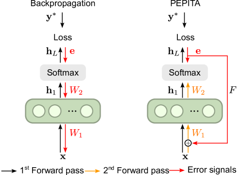
Figure 1: Comparison of BP and PEPITA. Schematic of BP’s and PEPITA’s architectures and learning mechanics with a single hidden layer.

In PEPITA, the gradients used to update the synaptic weights are then computed through the difference between the activations of the neurons in the first and second forward passes. If, for the first forward pass, the output of the network matches the target, the error signal $\mathbf{e}$ would be zero, and thus there would not be any synaptic weight updates because the neural activations in the second forward pass would not differ from the first forward pass. On the contrary, if the network made a wrong prediction in the first pass, then the neuronal activations in the second forward pass would differ, and the synaptic weights would be updated so that the mismatch is reduced. Note that for the last layer, the teaching signal is the error itself, which is why $\mathbf{e}$ is also fed directly to the output layer.

[tb] PEPITA’s Training Algorithm Given: input ($\mathbf{x}$), label ($\mathbf{y}^{*}$), and an activation function for each layer ($\sigma_{i}$) # Standard forward pass $\mathbf{h}_{0}=\mathbf{x}$ $i=1$ to $L$ $\mathbf{h}_{i}=\sigma_{i}(W_{i}\mathbf{h}_{i-1})$ $\mathbf{e}=\mathbf{h}_{L}-\mathbf{y}^{*}$ # Modulated forward pass $\mathbf{h}^{mod}_{0}=\mathbf{x}+F\mathbf{e}$ $i=1$ to $L$ $\mathbf{h}^{mod}_{i}=\sigma_{i}(W_{i}\mathbf{h}^{mod}_{i-1})$ $i<L$ $\Delta W_{i}=(\mathbf{h}_{i}-\mathbf{h}^{mod}_{i})\cdot(\mathbf{h}^{mod}_{i-1})^{T}$ $\Delta W_{L}=\textbf{e}\cdot(\mathbf{h}^{mod}_{L-1})^{T}$ # Update forward parameters with $\Delta W_{i}$ and an optimizer of choice

With this learning scheme, PEPITA sidesteps the biologically-implausible requirement of BP to backpropagate gradient information through the entire network hierarchical architecture, allowing the training of the synaptic weights to be based solely on spatially local information through a two-factor Hebbian-like learning rule. Therefore, while BP uses exact gradients for learning, that is, the exact derivative of the loss function with respect to its trainable parameters, PEPITA uses a very different learning mechanism that results in approximates of BP’s exact gradients.

To illustrate this difference, we write the explicit gradient weight updates for BP and PEPITA for the network represented in Figure 1. For the output layer, $W_{2}=W_{L}$, the synaptic weight updates of BP are computed as follows:

$$\Delta W^{BP}_{L} =\frac{\partial\mathcal{L}}{\partial W_{L}}=\frac{\partial\mathcal{L}}{\partial\mathbf{h}_{L}}\cdot\frac{\partial\mathbf{h}_{L}}{\partial W_{L}}$$ (1)

$$=\textbf{e}\cdot\left(\sigma_{L}^{\prime}(\mathbf{z}_{L})\cdot(\mathbf{h}_{L-1})^{T}\right),$$ (2)

where $\mathbf{z}_{L}=W_{L}\mathbf{h}_{L-1}$ and $\mathbf{e}=\partial\mathcal{L}/\partial\mathbf{h}_{L}$. For a simple mean-squared-error function (MSE) we have that $\mathbf{e}=\mathbf{h}_{L}-\mathbf{y}^{*}$. For the output layer weight updates, PEPITA leverages the same error signal and update structure as BP, the difference lying only on the scaling factor $\mathbf{z}_{L}$ and the pre-synaptic activation $\mathbf{h}^{mod}_{L-1}$ being given by the modulated forward pass:

$$\Delta W^{PEPITA}_{L}=\textbf{e}\cdot(\mathbf{h}^{mod}_{L-1})^{T}.$$ (3)

Hence, for the output layer, we have that $\Delta W^{PEPITA}_{L}\approx\Delta W^{BP}_{L}$, since the derivative of the activation function is bounded, and the difference between $\mathbf{h}^{mod}_{L-1}$ and $\mathbf{h}_{L-1}$ is small because the feedback projection matrix $F$ is scaled by a small constant, which guarantees that the perturbations added to the input are small [41]. On the contrary, considering the case with one hidden layer as illustrated in Figure 1, the synaptic weight updates of the hidden layer will differ more significantly since we have:

$$\Delta W^{BP}_{1}=\frac{\partial\mathcal{L}}{\partial W_{1}}=\frac{\partial\mathcal{L}}{\partial\mathbf{z}_{L}}\frac{\partial\mathbf{z}_{L}}{\partial\mathbf{z}_{1}}\frac{\partial\mathbf{z}_{1}}{\partial W_{1}}=\boldsymbol{\delta}_{1}\cdot\mathbf{x}^{T}$$ (4)

$$\Delta W^{PEPITA}_{1}=(\mathbf{h}_{1}-\mathbf{h}^{mod}_{1})\cdot(\mathbf{x}^{mod})^{T}$$ (5)

where $\boldsymbol{\delta}_{1}=(W_{2}^{T}\boldsymbol{\delta}_{2})\cdot\sigma_{1}^{\prime}(\mathbf{z}_{1})$ and $\boldsymbol{\delta}_{2}=\mathbf{e}$. In general, we can write $\Delta W^{BP}_{l}=\boldsymbol{\delta}_{l}\cdot\mathbf{h}_{l-1}^{T}$, where $\boldsymbol{\delta}_{l}$ is recursively obtained by writing it w.r.t. $\boldsymbol{\delta}_{l+1}$: $\boldsymbol{\delta}_{l}=(W_{l+1}^{T}\boldsymbol{\delta}_{l+1})\cdot\sigma_{l}^{\prime}(\mathbf{z}_{l})$.

Like BP, the FGSM and PGD adversarial attacks rely on backpropagating the exact derivatives of the loss function but all the way back to the input samples instead of just to the first hidden layer. For instance, the FGSM attack involves perturbing the input stimulus in the direction of the gradient of the loss function with respect to the input, being that the added perturbation is typically scaled by a small $\epsilon$ constant. An adversarial sample can computed as follows:

$$\mathbf{x}_{\text{adv}} =\mathbf{x}+\epsilon\cdot\text{sign}\Big{(}\frac{\partial\mathcal{L}}{\partial\mathbf{x}}\Big{)}$$ (6)

$$=\mathbf{x}+\epsilon\cdot\text{sign}\Big{(}\frac{\partial\mathcal{L}}{\partial\mathbf{z}_{L}}\frac{\partial\mathbf{z}_{L}}{\partial\mathbf{z}_{1}}\frac{\partial\mathbf{z}_{1}}{\partial\mathbf{x}}\Big{)}$$ (7)

$$=\mathbf{x}+\epsilon\cdot\text{sign}\Big{(}W_{1}^{T}\boldsymbol{\delta}_{1}\Big{)},$$ (8)

where $\mathbf{x}_{\text{adv}}$ is the adversarial example. Comparing Equations (8) and (4), we see that the driving signal, $\boldsymbol{\delta}_{1}$, is the same, and thus we postulate that the adversarial attacks have a more significant impact on BP-trained networks. The PGD attack follows a similar gradient path, applying FGSM iteratively with small stepsizes while projecting the perturbed input back into an $\epsilon$ ball. As PEPITA-trained models do not use these exact derivatives for learning, they form excellent candidates to be explored in the context of adversarial robustness. Note that, in the case of PEPITA, the attacker will still make use of the transposed feedforward pathway for computing the adversarial samples. Otherwise, if the random feedback projection matrix $F$ is used, the adversarial samples produced would be too weak, and the model could easily classify them correctly [50].

3 Results

3.1 Model training details

For our comparative study, we used four benchmark computer vision datasets: MNIST [42], Fashion-MNIST (F-MNIST) [43], CIFAR-$10$ and CIFAR-$100$ [44]. For both BP and PEPITA, we used the same network architectures and training schemes as described originally in Dellaferrera and Kreiman [41]. However, we added a bias to the hidden layer, as we observed a substantial performance improvement. The learning rule for this bias is similar to the one for the synaptic weights, but the pre-synaptic activation is fixed to one, i.e., $\mathbf{h}^{mod}_{i-1}\coloneqq\mathbf{1}$. Thus, similarly to the update rule for the synaptic weights (see Algorithm 1), the bias update rule can be written as $\Delta\mathbf{b}_{i}=(\mathbf{h}_{i}-\mathbf{h}^{mod}_{i})$ for $i<L$ and $\Delta\mathbf{b}_{L}=\mathbf{e}$. The network architecture consists of a single fully connected hidden layer with $1024$ ReLU neurons and a softmax output layer (as represented in Figure 1). For all the tasks, we used: the MSE loss, $100$ training epochs with early stopping, and the momentum Stochastic Gradient Descent (SGD) optimizer [45]. Furthermore, we used a mini-batch size of $64$, neuronal dropout of $10\%$, weight decay at epochs $60$ and $90$ with a rate of $0.1$, and the He uniform initialization [46] with the feedback projection matrix $F$ initialization scaled by $0.05$. 

We optimized the learning rate hyperparameter through a grid search over $50$ different values, and we defined the best-performing model as the model with the best natural accuracy on the validation dataset, consisting of natural samples the model has not yet seen. We chose this model selection criterion because, in real-world applications, the networks’ natural performance is most important to the user, and adversarial samples are considered outside of the norm. Thus, unless stated otherwise, we do not select the models based on the best adversarial validation accuracy, as we found that this comes at the cost of significantly worse natural performance. The values reported throughout this section are the mean $\pm$ standard deviation of the test accuracy for $5$ random seeds. The adversarial attacks were done using the open-source library $advertorch.attacks$ [47], which follows the original implementations of FGSM and PGD, as introduced in [5] and [20], respectively. We defined an attack step size of $0.1$ to create the FGSM and PGD adversarial samples and used $40$ iterations for PGD. Note that the maximum and minimum pixel values of the adversarial images are the same as for the original natural images.

3.2 Baseline natural and adversarial performance

Table 1 shows the models’ natural performance when trained naturally, without adversarial samples, and with natural validation accuracy as the hyperparameter selection criterion. In line with the results reported in the literature [41], PEPITA achieves a lower natural performance than BP. Notably, neither model is robust to adversarial attacks since neither has been adversarially trained nor has their hyperparameter selection criterion set to value adversarial robustness as an advantage.

		MNIST	Fashion-MNIST	CIFAR-10	CIFAR-100
BP	natural [%]	$98.58^{\pm 0.05}$	$90.52^{\pm 0.03}$	$57.05^{\pm 0.35}$	$27.54^{\pm 0.25}$
PEPITA	natural [%]	$98.16^{\pm 0.04}$	$86.46^{\pm 0.66}$	$52.15^{\pm 0.25}$	$25.88^{\pm 0.26}$

Table 1: Natural test accuracy. Here, the model is trained without adversarial samples, and the hyperparameter selection criterion is the natural validation accuracy.

3.3 PEPITA’s intrinsic higher adversarial robustness

When using the same training procedure as in the section above (natural training) but selecting the hyperparameter search criterion to value accuracy on adversarial validation samples, PEPITA shows a higher intrinsic adversarial robustness compared to BP – see Table 2. However, because of the natural-vs-adversarial performance trade-off, although this model selection criterion leads to a certain level of adversarial robustness for PEPITA (see row $4$ in Table 2), this comes at the cost of worsened natural performance (compared to row $2$ in Table 1). Nevertheless, when comparing the performance of BP with PEPITA for the MNIST dataset in Table 2, the natural performance of PEPITA decreases less than BP, and PEPITA is significantly more robust against adversarial attacks. Furthermore, BP-trained models cannot become adversarially robust with more complex tasks like Fashion-MNIST, CIFAR-$10$, and CIFAR-$100$. During the hyperparameter search of BP, it was observed that the learning rates tended to be much larger with the current selection criterion (best accuracy on adversarial validation samples). Consequently, the models either did not converge during learning, and the results were highly variable (see Table 2), or they did not learn at all, and the natural and adversarial performances became random.

		MNIST	Fashion-MNIST	CIFAR-10	CIFAR-100
BP	natural [%] PGD [%]	$94.22^{\pm 0.40}$ $92.72^{\pm 0.36}$	$43.82^{\pm 34.27}$ $22.89^{\pm 10.63}$	$10.003^{\pm 0.04}$ $9.98^{\pm 0.05}$	$9.078^{\pm 0.33}$ $0.33^{\pm 0.24}$
PEPITA	natural [%] PGD [%]	$97.69^{\pm 0.16}$ $97.56^{\pm 0.18}$	$80.65^{\pm 0.74}$ $80.48^{\pm 0.73}$	$41.82^{\pm 1.57}$ $41.73^{\pm 1.49}$	$17.10^{\pm 0.72}$ $16.76^{\pm 0.65}$

Table 2: Natural test accuracy and adversarial test accuracy with the PGD attack. Here, the model is trained without adversarial samples, and the hyperparameter selection criterion is the adversarial validation accuracy.

3.4 PEPITA’s advantageous adversarial training

When the models are now adversarially trained and the hyperparameter search selection criterion defined as the natural validation accuracy, we observe that PEPITA achieves a better adversarial testing performance and less natural performance degradation compared to BP (see Table 3), except for CIFAR-$100$ where both models are not significantly adversarially robust. Moreover, for the MNIST and Fashion-MNIST datasets, BP has better natural test accuracies. Hence, although Table 3 suggests that PEPITA offers a better natural-vs-adversarial performance trade-off, a direct comparison of the adversarial robustness between BP and PEPITA becomes difficult for these datasets. To better understand this trade-off, we selected the most adversarially robust BP-trained and PEPITA-trained models for different fixed natural accuracy values on the MNIST task. We plotted these results in Figure 2(A), which shows that PEPITA performs significantly better than BP for similar values of natural performance. Specifically, the average decrease in adversarial performance for the same values of natural performance is $0.26\%$ for PEPITA and $8.05\%$ for BP. Moreover, we verified that even if we double the number of training epochs for BP, its natural and adversarial accuracies remain approximately the same, indicating that the model has converged in its learning dynamics – see Figure 2(B). Hence, even after extensive hyperparameter searches and increased training epochs, we could not find BP-trained models with a better natural-vs-adversarial performance trade-off.

		MNIST	Fashion-MNIST	CIFAR-10	CIFAR-100
BP (PGD)	natural [%] PGD [%]	$98.73^{\pm 0.06}$ $89.93^{\pm 0.03}$	$85.16^{\pm 0.17}$ $67.42^{\pm 0.21}$	$35.83^{\pm 0.37}$ $8.58^{\pm 0.16}$	$12.45^{\pm 0.38}$ $2.11^{\pm 0.15}$
PEPITA (PGD)	natural [%] PGD [%]	$98.17^{\pm 0.10}$ $96.93^{\pm 0.41}$	$83.73^{\pm 0.76}$ $83.19^{\pm 0.68}$	$45.12^{\pm 0.89}$ $44.94^{\pm 0.83}$	$22.30^{\pm 0.16}$ $2.88^{\pm 1.74}$

Table 3: Natural test accuracy and adversarial test accuracy with the PGD attack. Here, the models are adversarially trained (i.e., trained with a dataset augmented by the adversarial samples) with PGD adversarial samples. The hyperparameter selection criterion is the natural validation accuracy.

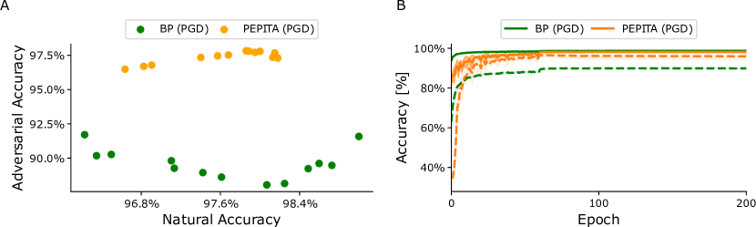
Figure 2: PEPITA’s advantageous adversarial training. The results presented here are for BP and PEPITA models trained adversarially with PGD samples on the MNIST task. (A) Natural-vs-adversarial performance trade-off: the most adversarially robust models were selected for different natural accuracy values. (B) Natural (represented by the full lines) and adversarial (represented by the dashed lines) accuracies of BP and PEPITA-trained models for double the amount of epochs.

3.5 PEPITA’s advantageous fast adversarial training

After demonstrating PEPITA’s intrinsic adversarial robustness and beneficial natural-vs-adversarial performance trade-off, we now investigate PEPITA’s capabilities in fast adversarial training [5]. Table 4 reports the results obtained when using fast adversarial training, i.e., when using FGSM adversarial samples for adversarial training, with the hyperparameter search selection criterion defined as the natural validation accuracy. For a visual representation of these results, refer to Figure 3. We observe that when attacking the trained models with strong attacks, such as with PGD adversarial samples, the decrease in adversarial performance is much less significant for PEPITA than for BP, indicating that the PEPITA-trained models overfit less to the FGSM attacks. Moreover, neither BP nor PEPITA-trained models suffer from catastrophic overfitting for this specific network architecture since the PGD testing accuracies do not drop to zero. This is the case because of two reasons: first, our network is over-parameterized for the tasks at hand, i.e., the network has more trainable parameters than there are samples in the dataset, so our large network width ($1024$ neurons) improves adversarial robustness; and second, we use He weights initialization, so our shallow network (a single hidden layer) also prevents a decrease in adversarial robustness [48]. To conclude, even if these models do not suffer from the extreme case of catastrophic overfitting, PEPITA has a more advantageous fast adversarial training since the gap between the FGSM and the PGD accuracies is much smaller for PEPITA than for BP.

		MNIST	Fashion-MNIST	CIFAR-10	CIFAR-100
BP (FGSM)	natural [%] FGSM [%] PGD [%]	$98.93^{\pm 0.05}$ $91.04^{\pm 0.13}$ $86.25^{\pm 0.09}$	$84.90^{\pm 0.03}$ $66.31^{\pm 0.25}$ $57.95^{\pm 0.33}$	$51.56^{\pm 0.43}$ $45.06^{\pm 3.38}$ $0.05^{\pm 0.04}$	$26.59^{\pm 0.08}$ $2.51^{\pm 0.37}$ $1.19^{\pm 0.08}$
PEPITA (FGSM)	natural [%] FGSM [%] PGD[%]	$98.00^{\pm 0.14}$ $97.91^{\pm 0.13}$ $97.81^{\pm 0.12}$	$80.70^{\pm 0.95}$ $80.68^{\pm 0.96}$ $80.27^{\pm 1.05}$	$41.22^{\pm 2.01}$ $41.22^{\pm 2.22}$ $41.00^{\pm 2.20}$	$17.89^{\pm 0.52}$ $17.68^{\pm 0.44}$ $17.53^{\pm 0.48}$

Table 4: Natural test accuracy and adversarial test accuracies with the PGD and FGSM attacks. Here, the models are adversarially trained with FGMS adversarial samples. The hyperparameter selection criterion is the natural validation accuracy.

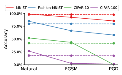
Figure 3: PEPITA’s advantageous fast adversarial training. The natural, FGMS, and PGD accuracies as reported in Table 4 for the models: BP (represented by the full lines) and PEPITA (represented by the dashed lines) when both are adversarially trained with FGMS adversarial samples.

3.6 Investigations on PEPITA’s adversarial robustness

Given our observations that PEPITA-trained models are more robust to adversarial attacks than BP-trained models, we aimed to investigate why this is the case. A crucial difference between both ANN learning algorithms is their gradient computation. While BP uses exact derivatives of the loss to compute the gradients used for learning (see Equations (1) and (4)), PEPITA uses alternative feedback and learning mechanisms that lead to approximations of these exact gradients [49] (see Equations (3) and (5)). To test the hypothesis that the error feedback signal shaping the approximate gradients of PEPITA, $\mathbf{h}_{i}-\mathbf{h}^{mod}_{i}$, is not just the teaching signal perturbed by some random noise but contains essential information for enhancing adversarial robustness, we added random noise to BP’s teaching signals and studied its adversarial robustness. We generated noise from a normal distribution with zero mean and a tunable standard deviation. We tested several hyperparameter combinations, including the standard deviation of the random noise, and none of the parameter settings led to increased adversarial robustness for BP. In particular, BP’s performance went from underperforming on classifying natural and adversarial samples for lower noise values to not being able to learn at all for higher noise values. Hence, we observe that a critical factor leading to adversarial robustness is how the gradients are computed during learning. As many biologically-plausible algorithms compute their gradients through feedback-based mechanisms that differ from BP, we can speculate that the resulting trained models possess better robustness against gradient-based adversarial attacks. Thus, an in-depth study of these could benefit the design of more adversarially robust models.

4 Discussion

Our paper demonstrates for the first time that biologically-inspired learning algorithms can lead to ANNs that are more robust against adversarial attacks than BP. We found that, unlike BP, PEPITA possesses intrinsic adversarial robustness. That is, naturally trained (i.e., only using natural samples) PEPITA models can be robust against adversarial attacks without the computationally heavy burden of adversarial training. A similar finding of intrinsic adversarial robustness has been demonstrated by Akrout [50] for the biologically-plausible learning algorithm Feedback Alignment (FA) [32]. However, in this previous work Akrout [50], a non-common practice that leads to much weaker adversarial attacks was used: the attackers use the FA’s random feedback matrices to generate adversarial samples instead of the transposed feedforward pathway. Hence, their analysis in Akrout [50] differs from our approach, where we let the attacker fully access the network architecture and synaptic weights and craft its adversarial samples through the transposed forward pathway. Moreover, we found that PEPITA does not suffer from the natural-vs-adversarial performance trade-off as severely as BP, as its models can be more adversarially robust than BP while losing less natural performance. Lastly, we found that PEPITA benefits much more from fast adversarial training than BP, i.e., when trained with samples generated from weaker adversarial attacks, it reports much better adversarial robustness against strong attacks.

Given that the link and the mathematical foundation between adversarial robustness and PEPITA have been established in this work, the next step would be to investigate further the theoretical understanding of PEPITA’s advantageous adversarial training and intrinsic adversarial robustness. With this understanding, the exact properties that improve the natural-vs-adversarial performance trade-off can be identified and leveraged for the development of other adversarially robust models. On another aspect, PEPITA has recently been extended to deeper networks (up to five hidden layers) and tested with different parameter initialization schemes [49], thus studying the impact of other characteristics of the model, such as width, depth, and initialization on PEPITA’s adversarial robustness would be beneficial (as done in [48]). PEPITA has also recently been combined with weight mirroring so that its feedback projection matrix can be learned [49], which improves natural performance, so it would be interesting to study whether this also improves adversarial robustness. While PEPITA, to our knowledge, was the first rate-based biologically-plausible learning algorithm being investigated regarding adversarial robustness, this kind of analysis should also be done for several other BP-alternative algorithms that have been proposed [33, 34, 35, 36, 38]. Hence, our work paves the way for a multitude of research directions to assess the properties that lead to adversarially robust models systematically.

4.1 Conclusion

To conclude, we demonstrated that ANNs trained with PEPITA, a recently proposed biologically-inspired learning algorithm, are more adversarially robust than BP-trained ANNs. In particular, we showed through several computational experiments that PEPITA significantly outperforms BP in an adversarial setting. Our analysis opens the door to drawing inspiration from biologically-plausible learning algorithms for designing more adversarially robust models. Thus, our work contributes to the creation of safer and more trustworthy artificial intelligence systems.

References

- Rumelhart et al. [1986] David E Rumelhart, Geoffrey E Hinton, and Ronald J Williams. Learning representations by back-propagating errors. Nature, 323(6088):533, 1986.
- Werbos [1982] Paul J Werbos. Applications of advances in nonlinear sensitivity analysis. In System modeling and optimization, pages 762–770. Springer, 1982.
- Madry et al. [2019] Aleksander Madry, Aleksandar Makelov, Ludwig Schmidt, Dimitris Tsipras, and Adrian Vladu. Towards Deep Learning Models Resistant to Adversarial Attacks, 2019. arXiv:1706.06083 [cs, stat].
- Szegedy et al. [2014] Christian Szegedy, Wojciech Zaremba, Ilya Sutskever, Joan Bruna, Dumitru Erhan, Ian Goodfellow, and Rob Fergus. Intriguing properties of neural networks, 2014. arXiv:1312.6199 [cs].
- Goodfellow et al. [2015] Ian Goodfellow, Jonathon Shlens, and Christian Szegedy. Explaining and harnessing adversarial examples. In International Conference on Learning Representations, 2015.
- Zhang et al. [2020] Wei Emma Zhang, Quan Sheng, Ahoud Alhazmi, and Chenliang Li. Adversarial attacks on deep-learning models in natural language processing: A survey. ACM Transactions on Intelligent Systems and Technology, 11:1–41, 2020. doi: 10.1145/3374217.
- Morris et al. [2020] John X. Morris, Eli Lifland, Jin Yong Yoo, Jake Grigsby, Di Jin, and Yanjun Qi. TextAttack: A Framework for Adversarial Attacks, Data Augmentation, and Adversarial Training in NLP, 2020. arXiv:2005.05909 [cs].
- Takahashi et al. [2021] Naoya Takahashi, Shota Inoue, and Yuki Mitsufuji. Adversarial attacks on audio source separation. In ICASSP 2021 - 2021 IEEE International Conference on Acoustics, Speech and Signal Processing (ICASSP), pages 521–525, 2021. doi: 10.1109/ICASSP39728.2021.9414844.
- Hussain et al. [2021] Shehzeen Hussain, Paarth Neekhara, Shlomo Dubnov, Julian McAuley, and Farinaz Koushanfar. WaveGuard: Understanding and Mitigating Audio Adversarial Examples, 2021. arXiv:2103.03344 [cs, eess].
- Gleave et al. [2020] Adam Gleave, Michael Dennis, Cody Wild, Neel Kant, Sergey Levine, and Stuart Russell. Adversarial Policies: Attacking Deep Reinforcement Learning. In International Conference on Learning Representations, 2020.
- Pattanaik et al. [2018] Anay Pattanaik, Zhenyi Tang, Shuijing Liu, Gautham Bommannan, and Girish Chowdhary. Robust deep reinforcement learning with adversarial attacks. In Proceedings of the 17th International Conference on Autonomous Agents and MultiAgent Systems, AAMAS ’18, page 2040–2042, 2018.
- Sarker [2021] Iqbal Sarker. Machine learning: Algorithms, real-world applications and research directions. SN Computer Science, 2, 03 2021. doi: 10.1007/s42979-021-00592-x.
- Akhtar and Mian [2018] Naveed Akhtar and Ajmal Mian. Threat of Adversarial Attacks on Deep Learning in Computer Vision: A Survey. IEEE, 6:14410–14430, 2018. ISSN 2169-3536. doi: 10.1109/ACCESS.2018.2807385.
- Eykholt et al. [2018] Kevin Eykholt, Ivan Evtimov, Earlence Fernandes, Bo Li, Amir Rahmati, Chaowei Xiao, Atul Prakash, Tadayoshi Kohno, and Dawn Song. Robust physical-world attacks on deep learning models, 2018. arXiv:1707.08945 [cs].
- Wang et al. [2022] Jia Wang, Chengyu Wang, Qiuzhen Lin, Chengwen Luo, Chao Wu, and Jianqiang Li. Adversarial attacks and defenses in deep learning for image recognition: A survey. Neurocomputing, 514:162–181, 2022. ISSN 0925-2312. doi: 10.1016/j.neucom.2022.09.004.
- Kaufmann et al. [2022] Maximilian Kaufmann, Yiren Zhao, Ilia Shumailov, Robert Mullins, and Nicolas Papernot. Efficient adversarial training with data pruning, 2022. arXiv:2207.00694 [cs].
- Addepalli et al. [2022] Sravanti Addepalli, Samyak Jain, and Venkatesh Babu R. Efficient and effective augmentation strategy for adversarial training. In Advances in Neural Information Processing Systems, volume 35, pages 1488–1501, 2022.
- Zheng et al. [2020] H. Zheng, Z. Zhang, J. Gu, H. Lee, and A. Prakash. Efficient adversarial training with transferable adversarial examples. In 2020 IEEE/CVF Conference on Computer Vision and Pattern Recognition (CVPR), pages 1178–1187. IEEE Computer Society, 2020. doi: 10.1109/CVPR42600.2020.00126.
- Sriramanan et al. [2021] Gaurang Sriramanan, Sravanti Addepalli, Arya Baburaj, and Venkatesh Babu R. Towards Efficient and Effective Adversarial Training. In Advances in Neural Information Processing Systems, volume 34, pages 11821–11833, 2021.
- Kurakin et al. [2016] Alexey Kurakin, Ian Goodfellow, and Samy Bengio. Adversarial examples in the physical world, 2016. arXiv:1607.02533 [cs].
- Wong et al. [2020] Eric Wong, Leslie Rice, and J. Zico Kolter. Fast is better than free: Revisiting adversarial training. In 8th International Conference on Learning Representations, ICLR, 2020.
- Kim et al. [2020] Hoki Kim, Woojin Lee, and Jaewook Lee. Understanding catastrophic overfitting in single-step adversarial training. In AAAI Conference on Artificial Intelligence, 2020.
- Golgooni et al. [2021] Zeinab Golgooni, Mehrdad Saberi, Masih Eskandar, and Mohammad Hossein Rohban. Zerograd: Mitigating and explaining catastrophic overfitting in fgsm adversarial training, 2021. arXiv.2103.15476 [cs].
- Kang and Moosavi-Dezfooli [2021] Peilin Kang and Seyed-Mohsen Moosavi-Dezfooli. Understanding catastrophic overfitting in adversarial training, 2021. arXiv:2105.02942 [cs].
- Tsipras et al. [2019] Dimitris Tsipras, Shibani Santurkar, Logan Engstrom, Alexander Turner, and Aleksander Madry. Robustness may be at odds with accuracy. In 7th International Conference on Learning Representations, ICLR, 2019.
- Zhang et al. [2019] Hongyang Zhang, Yaodong Yu, Jiantao Jiao, Eric P. Xing, Laurent El Ghaoui, and Michael I. Jordan. Theoretically principled trade-off between robustness and accuracy. In Proceedings of the 36th International Conference on Machine Learning, ICML, volume 97, pages 7472–7482, 2019.
- Moayeri et al. [2022] Mazda Moayeri, Kiarash Banihashem, and Soheil Feizi. Explicit Tradeoffs between Adversarial and Natural Distributional Robustness. In Advances in Neural Information Processing Systems, 2022.
- Zhou and Firestone [2019] Zhenglong Zhou and Chaz Firestone. Humans can decipher adversarial images. Nat. Commun., 10(1334):1–9, 2019. ISSN 2041-1723. doi: 10.1038/s41467-019-08931-6.
- Crick [1989] Francis Crick. The recent excitement about neural networks. Nature, 337(6203):129–132, 1989.
- Grossberg [1987] Stephen Grossberg. Competitive learning: From interactive activation to adaptive resonance. Cognitive Science, 11(1):23–63, 1987.
- Lillicrap et al. [2020] Timothy P Lillicrap, Adam Santoro, Luke Marris, Colin J Akerman, and Geoffrey Hinton. Backpropagation and the brain. Nature Reviews Neuroscience, pages 1–12, 2020.
- Lillicrap et al. [2016] Timothy P Lillicrap, Daniel Cownden, Douglas B Tweed, and Colin J Akerman. Random synaptic feedback weights support error backpropagation for deep learning. Nature Communications, 7:13276, 2016.
- Lee et al. [2015] Dong-Hyun Lee, Saizheng Zhang, Asja Fischer, and Yoshua Bengio. Difference target propagation. In Joint european conference on machine learning and knowledge discovery in databases, pages 498–515. Springer, 2015.
- Whittington and Bogacz [2017] James CR Whittington and Rafal Bogacz. An approximation of the error backpropagation algorithm in a predictive coding network with local hebbian synaptic plasticity. Neural computation, 29(5):1229–1262, 2017.
- Scellier and Bengio [2017] Benjamin Scellier and Yoshua Bengio. Equilibrium propagation: Bridging the gap between energy-based models and backpropagation. Frontiers in computational neuroscience, 11:24, 2017.
- Sacramento et al. [2018] João Sacramento, Rui Ponte Costa, Yoshua Bengio, and Walter Senn. Dendritic cortical microcircuits approximate the backpropagation algorithm. In Advances in Neural Information Processing Systems 31, pages 8721–8732, 2018.
- Akrout et al. [2019] Mohamed Akrout, Collin Wilson, Peter Humphreys, Timothy Lillicrap, and Douglas B Tweed. Deep learning without weight transport. In Advances in Neural Information Processing Systems 32, pages 974–982, 2019.
- Meulemans et al. [2021] Alexander Meulemans, Matilde Tristany Farinha, Javier García Ordóñez, Pau Vilimelis Aceituno, João Sacramento, and Benjamin F Grewe. Credit assignment in neural networks through deep feedback control. In Advances in Neural Information Processing Systems, 2021.
- Hinton [2022] Geoffrey Hinton. The Forward-Forward Algorithm: Some Preliminary Investigations, 2022. arXiv:2212.13345 [cs].
- Bohnstingl et al. [2022] Thomas Bohnstingl, Stanisław Woźniak, Angeliki Pantazi, and Evangelos Eleftheriou. Online Spatio-Temporal Learning in Deep Neural Networks. IEEE Transactions on Neural Networks and Learning Systems, pages 1–15, 2022. ISSN 2162-2388. doi: 10.1109/TNNLS.2022.3153985.
- Dellaferrera and Kreiman [2022] Giorgia Dellaferrera and Gabriel Kreiman. Error-driven input modulation: Solving the credit assignment problem without a backward pass. In Proceedings of the 39th International Conference on Machine Learning, volume 162, pages 4937–4955. PMLR, 2022.
- LeCun [1998] Yann LeCun. The mnist database of handwritten digits. http://yann. lecun. com/exdb/mnist/, 1998.
- Xiao et al. [2017] Han Xiao, Kashif Rasul, and Roland Vollgraf. Fashion-mnist: a novel image dataset for benchmarking machine learning algorithms, 2017. arXiv:1708.0774 [cs].
- Krizhevsky et al. [2014] Alex Krizhevsky, Vinod Nair, and Geoffrey Hinton. The CIFAR-10 dataset. online: http://www. cs. toronto. edu/kriz/cifar. html, 2014.
- Qian [1999] Ning Qian. On the momentum term in gradient descent learning algorithms. Neural Networks, 12(1):145–151, 1999. ISSN 0893-6080. doi: 10.1016/S0893-6080(98)00116-6.
- He et al. [2015] Kaiming He, Xiangyu Zhang, Shaoqing Ren, and Jian Sun. Delving deep into rectifiers: Surpassing human-level performance on imagenet classification. In 2015 IEEE International Conference on Computer Vision (ICCV), pages 1026–1034, 2015. doi: 10.1109/ICCV.2015.123.
- Ding et al. [2019] Gavin Weiguang Ding, Luyu Wang, and Xiaomeng Jin. advertorch v0.1: An adversarial robustness toolbox based on pytorch, 2019. arXiv:1902.07623 [cs].
- Zhu et al. [2022] Zhenyu Zhu, Fanghui Liu, Grigorios G. Chrysos, and Volkan Cevher. Robustness in deep learning: The good (width), the bad (depth), and the ugly (initialization). In Advances in neural information processing systems, 2022.
- Srinivasan et al. [2023] Ravi Francesco Srinivasan, Francesca Mignacco, Martino Sorbaro, Maria Refinetti, Avi Cooper, Gabriel Kreiman, and Giorgia Dellaferrera. Forward Learning with Top-Down Feedback: Empirical and Analytical Characterization, 2023. arXiv:2302.05440 [cs].
- Akrout [2019] Mohamed Akrout. On the adversarial robustness of neural networks without weight transport, 2019. arXiv:1908.03560 [cs].