Symmetric Bernoulli distributions and minimal dependence copulas

Abstract

The key result of this paper is to find all the joint distributions of random vectors whose sums $S=X_{1}+\ldots+X_{d}$ are minimal in convex order in the class of symmetric Bernoulli distributions. The minimal convex sums distributions are known to be strongly negatively dependent. Beyond their interest per se, these results enable us to explore negative dependence within the class of copulas. In fact, there are two classes of copulas that can be built from multivariate symmetric Bernoulli distributions: the extremal mixture copulas, and the FGM copulas. We study the extremal negative dependence structure of the copulas corresponding to symmetric Bernoulli vectors with minimal convex sums and we explicitly find a class of minimal dependence copulas. Our main results stem from the geometric and algebraic representations of multivariate symmetric Bernoulli distributions, which effectively encode several of their statistical properties.

Keywords: Symmetric Bernoulli distributions, FGM copulas, extremal mixture copulas, convex order, negative dependence.

Introduction

A problem extensively studied in applied probability is finding bounds for sums $S=X_{1}+\ldots+X_{d}$ of random variables with joint distribution in a given Fréchet class $\mathcal{F}(F_{1},\ldots,F_{d})$, i.e. the class of all the joint distributions with one-dimensional $i$-th marginal distribution $F_{i}$ (see e.g. [1], [2], [3], [4]). In insurance and finance relevant bounds are in convex order, a stochastic order that is used to express which of two risks is higher. The problem of finding the upper bound is solved: the upper bound is reached when the risks are co-monotone and their joint distribution is the upper Fréchet bound, that is the maximum element -in concordance order- of $\mathcal{F}(F_{1},\ldots,F_{d})$ [5]. The problem of finding the lower bound is not as straightforward: in dimension two the solution is the lower Fréchet bound, the joint distribution of counter-monotone bivariate random vector, but if $d\geq 3$ it fails to be a distribution (see [6]). The problem of finding distributions in $\mathcal{F}(F_{1},\ldots,F_{d})$ corresponding to minimal aggregate risk is still as yet unsolved in general and this is the problem we focus on. Following [7] we call the random vectors with minimal convex sums and their distributions the $\Sigma_{cx}$-smallest elements of $\mathcal{F}(F_{1},\ldots,F_{d})$, when they exist.

We consider two Fréchet classes. One is the class $\mathcal{SB}_{d}$ of multidimensional distributions with one-dimensional Bernoulli marginals with mean $p=1/2$, called multivariate symmetric Bernoulli distributions. The other class is whole class of copulas, i.e. the class of multivariate distribution functions with one-dimensional uniform marginals [8]. We solve the problem of finding all $\Sigma_{cx}$-smallest elements in the Fréchet class $\mathcal{SB}_{d}$ by generalizing the results in [9], where the unique exchangeable $\Sigma_{cx}$-smallest element is found and in [10] where one specific non-exchangeable $\Sigma_{cx}$-smallest element is found. In fact, both these results hold in the more general Fréchet class $\mathcal{F}_{d}(p)$ of $d$-dimensional Bernoulli distributions with the same one-dimensional marginals with mean $p$.

In [7] the authors prove that if $\boldsymbol{X}$ has a $\Sigma_{cx}$-smallest distribution than it is $\Sigma$-countermonotonic, a multivariate extension of the bivariate counter-monotonicity, that is the maximal negative dependence between two random variables (see [11]). As a consequence, the $\Sigma_{cx}$-smallest elements in $\mathcal{SB}_{d}$ define a class of extremely negative dependent symmetric Bernoulli vectors. Although these results are of interest per se, they contribute to the study of negative dependence in a more general framework. In fact, they allow us to explicitly find a class of $\Sigma$-countermonotonic copulas, i.e. minimal dependence copulas. Extreme negative dependence and its relationship with minimal risk is extensively studied in the context of insurance and finance (see, among others, [11], [12], [13]). In this framework, the theory of copulas provides a useful tool to model dependence and to find distributional bounds for dependent risks ([14]).

There are two classes of copulas that can be built from multivariate symmetric Bernoulli distributions: the extremal mixture copulas [15], and the Farlie-Gumbel-Morgenstern (FGM) copulas [16]. While FGM copulas are in a one to one relationship with the elements of the class $\mathcal{SB}_{d}$, the extremal mixture copulas are in a one to one relationship with the subclass of palindromic Bernoulli distributions. We study the dependence structure of the copulas corresponding to $\Sigma_{cx}$-smallest Bernoulli distributions in these two classes. This paper proves that the extremal copulas -a subclass of the extremal mixture copulas- corresponding to the $\Sigma_{cx}$-smallest elements of $\mathcal{SB}_{d}$ are $\Sigma$-countermonotonic. This result can be improved when the dimension of the Fréchet class $d$ is even: in this case, the extremal mixture copulas corresponding to $\Sigma_{cx}$-smallest Bernoulli distributions are also the $\Sigma_{cx}$-smallest elements in the Fréchet class of copulas ([7]). Therefore if $d$ is even, multivariate uniform variables have a minimum risk element. Finally, we study the FGM copulas corresponding to the $\Sigma_{cx}$-smallest elements in $\mathcal{SB}_{d}$ employing widely used measures of dependence: Person’s rho, Spearman’s rho and Kendall’s tau.

Our results follow from the geometrical and algebraic representations of the class $\mathcal{SB}_{d}$. This class can be represented as a convex polytope (see [17]) whose extremal generators encode relevant statistical properties, such as extremal dependence or distributional bounds for relevant risk measures. While extremal generators can be found in closed form in special classes (see [18]) and analytically in low dimension, finding them in high dimension become computationally infeasible. For this reason, in [10] the authors find a way around this limitation and map the class of multivariate Bernoulli distributions with given mean $p$ into an ideal of points in the ring of polynomials with rational coefficients. Using the results in [10] we find an analytical set of polynomials that generates the class $\mathcal{SB}_{d}$ and an analytical set of polynomials that generates the class of palindromic distributions. These last generators are extremal points of the polytope and they are associated to the extremal copulas. These connections allow us to find the $\Sigma$-countermonotonic extremal copulas. Indeed, the effectiveness of the algebraic representation is that the polynomial coefficients can be used to construct multivariate Bernoulli distributions with given statistical properties.

The paper is organized as follows. Section 1 introduces the notation and recalls the geometrical representation of $\mathcal{SB}_{d}$. Section 2 introduces the algebraic representation of the class $\mathcal{SB}_{d}$, proves some new results that connect the algebraic and the geometrical generators, and characterize the palindromic Bernoulli distributions. The $\Sigma_{cx}$-smallest elements of $\mathcal{SB}_{d}$ and of the palindromic subclass are found in Section 3. Section 4 focuses on the extremal mixture copulas, a subclass of extremal copulas and find the $\Sigma$-countermonotonic copulas. Section 5 introduces the FGM copulas and investigates the dependence structure of the FGM copulas corresponding to $\Sigma_{cx}$-smallest elements in $\mathcal{SB}_{d}$ using dependence measures, such as Person’s rho, Spearman’s rho and Kendall’s tau. Concluding remarks are made in Section 6.

1
Notation and Preliminaries

Let $\mathcal{F}_{d}$ be the set of $d$-dimensional probability mass functions (pmfs) which have Bernoulli univariate marginal distributions. Let us consider the Fréchet class $\mathcal{F}_{d}(p)\subseteq\mathcal{F}_{d}$ of pmfs in $\mathcal{F}_{d}$ which have the same Bernoulli marginal distributions of parameter $p$, $B(p)$. We assume throughout the paper that $p$ is rational, i.e. $p\in\mathbb{Q}$. Since $\mathbb{Q}$ is dense in $\mathbb{R}$, this is not a limitation in applications. Since we focus on symmetric Bernoulli distributions we define $\mathcal{SB}_{d}=\mathcal{F}_{d}(\tfrac{1}{2})$ to be the Fréchet class of $d$-dimensional Bernoulli distributions with marginals distributed as Bernoulli with mean $\tfrac{1}{2}$.

We assume that vectors are column vectors and we denote by $A^{\top}$ the transpose of a matrix $A$. If $\boldsymbol{X}=(X_{1},\dots,X_{d})$ is a random vector with pmf in $\mathcal{F}_{d}$, we denote

• its cumulative distribution function by $F$ and its mass function by $f$;

• the column vector which contains the values of $F$ and $f$ over $\mathcal{X}_{d}=\{0,1\}^{d}$, by $\boldsymbol{F}=(F_{1},\ldots,F_{D}):=(F(\boldsymbol{x}):\boldsymbol{x}\in\mathcal{X}_{d})$, and $\boldsymbol{f}=(f_{1},\ldots,f_{2^{d}}):=(f(\boldsymbol{x}):\boldsymbol{x}\in\mathcal{X}_{d})$, respectively; we make the non-restrictive hypothesis that the set $\mathcal{X}_{d}$ of $2^{d}$ binary vectors is ordered according to the reverse-lexicographical criterion. For example we have $\mathcal{S}_{3}=\{000,100,010,110,001,101,011,111\}$.

The notation $\boldsymbol{X}\in\mathcal{F}_{d}(p)$, $\boldsymbol{F}\in\mathcal{F}_{d}(p)$ and $\boldsymbol{f}\in\mathcal{F}_{d}(p)$ indicates that $\boldsymbol{X}$ has pmf $f\in\mathcal{F}_{d}(p)$.

Given two matrices $A\in\mathcal{M}(n\times m)$ and $B\in\mathcal{M}(d\times l)$:

• if $n=d$, $A||B$ denotes the row concatenation of $A$ and $B$;

• if $m=l$, $A//B$ denotes the column concatenation of $A$ and $B$;

Finally, we denote by $P(\boldsymbol{z})=\sum_{\boldsymbol{i}\in\{0,1\}^{d-1}}a_{\boldsymbol{i}}\boldsymbol{z}^{\boldsymbol{i}}$ a polynomial in the ring $\mathbb{Q}[\boldsymbol{z}]$ of polynomials with rational coefficients in the variables $\boldsymbol{z}=(z_{1},\ldots,z_{d-1})$, where $\boldsymbol{z}^{\boldsymbol{i}}=\prod_{j=1}^{d-1}z_{j}^{i_{j}}$. To simplify the notation we write $a_{i_{1}\dots i_{d-1}}:=a_{(i_{1},\ldots,i_{d-1})}=a_{\boldsymbol{i}}$.

In [17], the authors show that $\mathcal{SB}_{d}$ is a convex polytope:

$$\mathcal{SB}_{d}=\bigg{\{}\boldsymbol{f}\in\mathbb{R}^{2^{d}}:H_{d}\boldsymbol{f}=\boldsymbol{0},f_{j}\geq 0,\sum_{j=1}^{2^{d}}f_{j}=1\bigg{\}},$$ (1.1)

where $H_{d}$ is a $d\times 2^{d}$ matrix whose rows are $(\boldsymbol{1}_{d}-2\boldsymbol{x}_{h})^{\top}$, $h\in\{1,\dots,d\}$ and $\boldsymbol{x}_{h}$ is the vector of the $h$-th elements of all the vectors $\boldsymbol{x}\in\mathcal{X}_{d}$. Therefore, for any $\boldsymbol{f}\in\mathcal{SB}_{d}$, there exist $n$ positive weights $\lambda_{1},\ldots,\lambda_{n}$ summing up to one and $n$ extremal points $\boldsymbol{r}_{i}\in\mathcal{SB}_{d}$ such that

$$\boldsymbol{f}=\sum_{i=1}^{n}\lambda_{i}\boldsymbol{r}_{i}.$$

We call $\boldsymbol{r}_{i}$ the extremal points of extremal pmfs.

Example 1.

Consider $d=3$. Then, $\boldsymbol{x}_{1}=(0,1,0,1,0,1,0,1)$, $\boldsymbol{x}_{2}=(0,0,1,1,0,0,1,1)$, and $\boldsymbol{x}_{3}=(0,0,0,0,1,1,1,1)$. The matrix that generates the class $\mathcal{SB}_{3}$ is

$$H_{3}=\begin{pmatrix}1&-1&1&-1&1&-1&1&-1\\ 1&1&-1&-1&1&1&-1&-1\\ 1&1&1&1&-1&-1&-1&-1\\ \end{pmatrix}.$$

The convex polytope has $n=6$ extremal points, that are reported in Table 1.

$\boldsymbol{x}$	$\boldsymbol{r}_{1}$	$\boldsymbol{r}_{2}$	$\boldsymbol{r}_{3}$	$\boldsymbol{r}_{4}$	$\boldsymbol{r}_{5}$	$\boldsymbol{r}_{6}$
$(0,0,0)$	0	0	0	0.5	0	0.25
$(0,1,0)$	0	0	0.5	0	0.25	0
$(1,0,0)$	0	0.5	0	0	0.25	0
$(1,1,0)$	0.5	0	0	0	0	0.25
$(0,0,1)$	0.5	0	0	0	0.25	0
$(1,0,1)$	0	0.5	0	0	0	0.25
$(0,1,1)$	0	0	0.5	0	0	0.25
$(1,1,1)$	0	0	0	0.5	0.25	0

Table 1: Extremal probability mass functions of the class $\mathcal{SB}_{3}$.

The above representation has computational limitation when the dimension increases, due to the growth of the number of extremal points of the convex cone. To overcame this limitation in [10] the authors introduce a new algebraic representation of the class $\mathcal{F}_{d}(p)$, that proves to be extremely effective to study the case $p=\tfrac{1}{2}$. We recall this representation in the following Section 2 and then we state a list of new results for the special case under consideration, i.e. $p=\tfrac{1}{2}$.

2
Algebraic representation

Following [10], we define the map $\mathcal{H}$ from $\mathcal{SB}_{d}$ to the polynomial ring with rational coefficients $\mathbb{Q}[z_{1},\ldots,z_{d-1}]$ as:

$$\begin{split}\mathcal{H}:\quad\mathcal{SB}_{d}&\to\mathbb{Q}[z_{1},\ldots,z_{d-1}]\\ \boldsymbol{f}&\mapsto\mathcal{H}(\boldsymbol{f})=\sum_{\boldsymbol{i}\in\{0,1\}^{d-1}}a_{\boldsymbol{i}}\boldsymbol{z}^{\boldsymbol{i}}.\end{split}$$

We call $\mathcal{C_{H}}$ the image of $\mathcal{SB}_{d}$ through $\mathcal{H}$. From Theorem 3.1 in [10], $\mathcal{C_{H}}\subseteq\mathcal{I}_{\mathcal{P}},$ where $\mathcal{I}_{\mathcal{P}}\subseteq\mathbb{Q}[\boldsymbol{z}]$ is the ideal of polynomials that vanish at points $\mathcal{P}=\{\boldsymbol{1}_{d-1},\boldsymbol{1}_{d-1}^{-j},j=1,\ldots,d-1\}$, where $\boldsymbol{1}_{d-1}$ is a vector of ones of length $d-1$ and $\boldsymbol{1}_{d-1}^{-j}$ is a vector of length $d-1$ with $-1$ in position $j$ and $1$ elsewhere. The vector $\boldsymbol{a}$ of the $2^{d-1}$ coefficients of the polynomial is given by

$$\boldsymbol{a}=(a_{\boldsymbol{i}})_{\boldsymbol{i}\in\{0,1\}^{d-1}}=Q\boldsymbol{f},$$ (2.1)

with $Q=(I(2^{d-1})||\tilde{I}(2^{d-1}))$, where $I(2^{d-1})$ is the identity matrix of order $2^{d-1}$ and $\tilde{I}(2^{d-1})$ is the square matrix of order $2^{d-1}$ with $-1$ on the anti-diagonal. For every $\boldsymbol{i}\in\{0,1\}^{d-1}$, set $\boldsymbol{s}_{\boldsymbol{i}}:=(\boldsymbol{i},0)=(i_{1},\ldots,i_{d-1},0)$. Then, we have $\boldsymbol{1}_{d}-\boldsymbol{s}_{\boldsymbol{i}}=(1-i_{1},\ldots,1-i_{d-1},1)$. Let $a_{\boldsymbol{i}}^{+}:=f(\boldsymbol{s}_{\boldsymbol{i}})=\mathbb{P}(\boldsymbol{X}=\boldsymbol{s}_{\boldsymbol{i}})$ be the probability of realization of $\boldsymbol{s}_{\boldsymbol{i}}$, and let $a_{\boldsymbol{i}}^{-}:=f(\boldsymbol{1}_{d}-\boldsymbol{s}_{\boldsymbol{i}})=\mathbb{P}(\boldsymbol{X}=\boldsymbol{1}_{d}-\boldsymbol{s}_{\boldsymbol{i}})$. Thus, we can write Equation (2.1) as:

$$a_{\boldsymbol{i}}=a_{(i_{1},\ldots,i_{d-1})}=f(\boldsymbol{s}_{\boldsymbol{i}})-f(\boldsymbol{1}_{d}-\boldsymbol{s}_{\boldsymbol{i}})=a_{\boldsymbol{i}}^{+}-a_{\boldsymbol{i}}^{-},$$ (2.2)

for every $\boldsymbol{i}=(i_{1},\ldots,i_{d-1})\in\{0,1\}^{d-1}$.

Example 2.

We consider the case $d=3$, $\mathcal{SB}_{3}$. We have $\boldsymbol{a}=Q\boldsymbol{f}$, where

$$\boldsymbol{a}=\begin{pmatrix}a_{00}\\ a_{10}\\ a_{01}\\ a_{11}\\ \end{pmatrix},\quad Q=\begin{pmatrix}1&0&0&0&0&0&0&-1\\ 0&1&0&0&0&0&-1&0\\ 0&0&1&0&0&-1&0&0\\ 0&0&0&1&-1&0&0&0\\ \end{pmatrix},\quad\boldsymbol{f}=\begin{pmatrix}f_{000}\\ f_{100}\\ f_{010}\\ f_{110}\\ f_{001}\\ f_{101}\\ f_{011}\\ f_{111}\\ \end{pmatrix}.$$

Therefore, for $d=3$, the polynomials in $\mathcal{C}_{\mathcal{H}}\subseteq\mathcal{I}_{\mathcal{P}}$ are of the form $P(\boldsymbol{z})=a_{00}+a_{10}z_{1}+a_{01}z_{2}+a_{11}z_{1}z_{2}$, where

$$\begin{cases}a_{00}=f_{000}-f_{111}\\ a_{10}=f_{100}-f_{011}\\ a_{01}=f_{010}-f_{101}\\ a_{11}=f_{110}-f_{001}\\ \end{cases}.$$

The polynomials in $\mathcal{I}_{\mathcal{P}}$ vanish at points $\boldsymbol{z}=\boldsymbol{1}_{d-1}=(1,1)$, $\boldsymbol{z}=\boldsymbol{1}_{d-1}^{-1}=(-1,1)$ and $\boldsymbol{z}=\boldsymbol{1}_{d-1}^{-2}=(1,-1)$. For example, let us consider the following pmfs and their corresponding polynomials $\mathcal{H}(\boldsymbol{f})$:

$$\begin{split}&\boldsymbol{f}_{1}=(0.3,0.1,0.1,0,0.1,0,0,0.4),\\ &\boldsymbol{f}_{2}=(0.1,0.1,0.1,0.2,0.3,0,0,0.2),\\ &\boldsymbol{f}_{3}=(0,0.25,0.25,0,0.25,0,0,0.25),\\ &\boldsymbol{f}_{4}=(0.25,0,0,0.25,0,0.25,0.25,0),\end{split}\qquad\begin{split}&P_{1}(\boldsymbol{z})=-0.1+0.1z_{1}+0.1z_{2}-0.1z_{1}z_{2};\\ &P_{2}(\boldsymbol{z})=-0.1+0.1z_{1}+0.1z_{2}-0.1z_{1}z_{2};\\ &P_{3}(\boldsymbol{z})=-0.25+0.25z_{1}+0.25z_{2}-0.25z_{1}z_{2};\\ &P_{4}(\boldsymbol{z})=0.25-0.25z_{1}-0.25z_{2}+0.25z_{1}z_{2}.\end{split}$$

The polynomials $P_{1}(\boldsymbol{z})$ and $P_{2}(\boldsymbol{z})$ are identical, while $P_{3}(\boldsymbol{z})=\frac{5}{2}\cdot P_{1}(\boldsymbol{z})$ and $P_{4}(\boldsymbol{z})=-P_{3}(\boldsymbol{z})$.

Fontana and Semeraro (see [10]) prove that the map $\mathcal{H}$ is not injective -as explicitly shown in Example 2- and they find a basis of the kernel $\mathcal{K}(\mathcal{H})$ of the map, i.e. the set of pmfs $\boldsymbol{f}$ such that $\mathcal{H}(\boldsymbol{f})=0$. In the case $p=\frac{1}{2}$, a basis of the kernel is the set:

$$\mathcal{B}_{K}=\big{\{}\big{(}\tfrac{1}{2},0,0,\ldots,0,0,\tfrac{1}{2}\big{)};\big{(}0,\tfrac{1}{2},0,\ldots,0,\tfrac{1}{2},0\big{)};\big{(}0,0,\tfrac{1}{2},\ldots,\tfrac{1}{2},0,0\big{)};\ldots\big{\}}.$$ (2.3)

A subclass of Bernoulli distributions in $\mathcal{SB}_{d}$ characterized by the kernel is the class $\mathcal{PB}_{d}$ of palindromic Bernoulli distribution, i.e. the distributions of the Bernoulli random variables $\boldsymbol{X}$ such that $\mathbb{P}(\boldsymbol{X}=\boldsymbol{x})=\mathbb{P}(\boldsymbol{X}=\boldsymbol{1}_{d}-\boldsymbol{x})$, for every $\boldsymbol{x}\in\{0,1\}^{d}$ (see e.g. [19] as a reference for palindromic distributions). The proofs of the following propositions are straightforward, yet the results are important to our purposes, because palindromic Bernoulli distributions generate the class of extremal mixture copulas [15], which are one of our objects of study.

Proposition 2.1.

The kernel of the map $\mathcal{H}$ coincides with the set of the palindromic Bernoulli distributions, $\mathcal{K}(\mathcal{H})\equiv\mathcal{PB}_{d}$.

Proposition 2.2.

The pmfs of the basis $\mathcal{B}_{K}$ of the kernel of $\mathcal{H}$ in Equation (2.3) are extremal points of the polytope $\mathcal{SB}_{d}$.

Proof.

The pmfs in $\mathcal{B}_{K}$ have mass on two points only. Let us suppose that a pmf $\boldsymbol{f}_{K}$ of $\mathcal{B}_{K}$ is not extremal. Therefore, there exists an extremal pmf $\boldsymbol{f}_{E}$ whose support is contained in the support of $\boldsymbol{f}_{K}$, as a consequence of Lemma 2.4 in [20]. This extremal pmf should have support on one point only and this is not consistent with the condition on the mean $p=1/2$. ∎

The basis $\mathcal{B}_{K}$ has $2^{d-1}$ pmfs, therefore, there are $2^{d-1}$ extremal pmfs that have null polynomial.

The kernel of the map $\mathcal{H}$ is now fully characterized. It is more challenging to characterize the counter-image of a non-null polynomial. In [10], the authors suggest an algorithm to find a particular distribution from a given polynomial, which they call the type-0 probability mass function. The algorithm for $p=\tfrac{1}{2}$ is reported in Table 2. This result can be improved for the class $\mathcal{SB}_{d}$.

Algorithm 1

Input: A polynomial $P(\boldsymbol{z})=\sum_{\boldsymbol{i}\in\{0,1\}^{d-1}}a_{\boldsymbol{i}}\boldsymbol{z}^{\boldsymbol{i}}\in\mathcal{I}_{\mathcal{P}}$.

For each $\boldsymbol{i}\in\{0,1\}^{d-1}$:

if $a_{\boldsymbol{i}}\geq 0$, then $f_{P}(\boldsymbol{s}_{\boldsymbol{i}})=a_{j}$ and $f_{P}(\boldsymbol{1}_{d}-\boldsymbol{s}_{\boldsymbol{i}})=0$;

if $a_{\boldsymbol{i}}<0$, then $f_{P}(\boldsymbol{s}_{\boldsymbol{i}})=0$ and $f_{P}(\boldsymbol{1}_{d}-\boldsymbol{s}_{\boldsymbol{i}})=a_{j}$.

Normalize $\boldsymbol{f}_{P}$ getting, with a small abuse of notation, $\boldsymbol{f}_{P}=\boldsymbol{f}_{P}/(\sum_{\boldsymbol{x}\in\{0,1\}^{d}}f_{P}(\boldsymbol{x}))$.

Output: A pmf $\boldsymbol{f}=(f_{1},\ldots,f_{2^{d}})\in\mathcal{F}_{d}(1/2)$.

Table 2: Algorithm to generate the type-0 probability mass function associated to $P(\boldsymbol{z})$.

The following definition introduces the concept of equivalence between polynomials of the ideal $\mathcal{I}_{\mathcal{P}}$.

Definition 2.1.

Two polynomials $P(\boldsymbol{z})$ and $Q(\boldsymbol{z})$ of the ideal $\mathcal{I}_{\mathcal{P}}$ are equivalent, that is, $P(\boldsymbol{z})\simeq Q(\boldsymbol{z})$, if there exists a constant $\mu>0$, $\mu\in\mathbb{Q}$, such that $P(\boldsymbol{z})=\mu Q(\boldsymbol{z})$. We define $[P(\boldsymbol{z})]=\{Q(\boldsymbol{z})\in\mathcal{I}_{\mathcal{P}}:Q(\boldsymbol{z})\simeq P(\boldsymbol{z})\}$ as the set of all the polynomials equivalent to $P(\boldsymbol{z})$

Example 3.

Considering the four vectors of Example 2, we have $P_{1}(\boldsymbol{z})\simeq P_{2}(\boldsymbol{z})\simeq P_{3}(\boldsymbol{z})$. Instead, $P_{4}(\boldsymbol{z})$ is not equivalent to the other polynomials.

The following proposition holds in general for any Fréchet class $\mathcal{F}_{d}(p)$.

Proposition 2.3.

Two equivalent polynomials generate the same type-0 pmf.

Proof.

Let $P(\boldsymbol{z})$ and $Q(\boldsymbol{z})$ be two equivalent polynomials and let $\boldsymbol{f}_{P}$ and $\boldsymbol{f}_{Q}$ be the two corresponding type-0 pmfs. Then there exists $\mu>0$ such that $P(\boldsymbol{z})=\mu Q(\boldsymbol{z})$. Apply Algorithm 1 both to $P(\boldsymbol{z})$ and to $Q(\boldsymbol{z})$ (for $p\neq\tfrac{1}{2}\in\mathbb{Q}$ see the version of Algorithm 1 in [10]). The coefficients of the two polynomials have the same sign, therefore, after the first step of the algorithm, we have $\boldsymbol{f}_{P}=\mu\boldsymbol{f}_{Q}$. After normalization, we have that the two type-0 pmfs are identical. ∎

Given a polynomial $P(\boldsymbol{z})$, the following Proposition 2.4 characterizes all the pmfs mapped by $\mathcal{H}$ in a polynomial equivalent to $P(\boldsymbol{z})$, i.e. all the pmfs $\boldsymbol{f}$ such that $\mathcal{H}(\boldsymbol{f})\in[P(\boldsymbol{z})]$. Let us define $\mathcal{H}^{-1}[P(\boldsymbol{z})]:=\big{\{}\boldsymbol{f}\in\mathcal{SB}_{d}:\mathcal{H}(\boldsymbol{f})\in[P(\boldsymbol{z})]\big{\}}$.

Proposition 2.4.

Given a polynomial $P(\boldsymbol{z})=\sum_{\boldsymbol{i}\in\{0,1\}^{d-1}}a_{\boldsymbol{i}}\boldsymbol{z}^{\boldsymbol{i}}\in\mathcal{I}_{\mathcal{P}}$, such that $P(\boldsymbol{z})\neq 0$, then

$$\mathcal{H}^{-1}[P(\boldsymbol{z})]=\big{\{}\boldsymbol{f}\in\mathcal{SB}_{d}:\boldsymbol{f}=\lambda\boldsymbol{f}_{P}+(1-\lambda)\boldsymbol{e}_{K}\text{, with }\boldsymbol{e}_{K}\in\mathcal{K}(\mathcal{H}),\lambda\in(0,1]\big{\}},$$

where $\boldsymbol{f}_{P}$ is the type-0 pmf of $P(\boldsymbol{z})$.

Proof.

Let $A=\{\boldsymbol{f}\in\mathcal{SB}_{d}:\boldsymbol{f}=\lambda\boldsymbol{f}_{P}+(1-\lambda)\boldsymbol{e}_{K}\text{, with }\boldsymbol{e}_{K}\in\mathcal{K(H)},\lambda\in(0,1]\}$, where $\boldsymbol{f}_{P}$ is the type-0 pmf of $[P(\boldsymbol{z})]$ and let $\mathcal{H}(\boldsymbol{f}_{P})=P(\boldsymbol{z})$. The map $\mathcal{H}$ is linear, therefore $\mathcal{H}(\boldsymbol{f})=\mathcal{H}(\lambda\boldsymbol{f}_{P}+(1-\lambda)\boldsymbol{e}_{K})=\lambda\mathcal{H}(\boldsymbol{f}_{P})+(1-\lambda)\mathcal{H}(\boldsymbol{e}_{K})=\lambda P(\boldsymbol{z})$, and we have $A\subseteq\mathcal{H}^{-1}[P(\boldsymbol{z})]$. Let $\boldsymbol{f}\in\mathcal{H}^{-1}[P(\boldsymbol{z})]$. We want to prove that $\boldsymbol{f}$ can be written as a convex linear combination between $\boldsymbol{f}_{P}$ and an element of the kernel of $\mathcal{H}$. Let $Q(\boldsymbol{z})=\mathcal{H}(\boldsymbol{f})$. By definition of the inverse map $\mathcal{H}^{-1}$, there exists $\mu>0$ such that $\mathcal{H}(\boldsymbol{f})=\mu\mathcal{H}(\boldsymbol{f}_{P})$, that is $Q(\boldsymbol{z})=\mu P(\boldsymbol{z})$. Hence, to prove that $\boldsymbol{f}=\mu\boldsymbol{f}_{P}+(1-\mu)\boldsymbol{e}_{K}$, we need to prove that $\boldsymbol{e}_{K}=\frac{1}{1-\mu}\boldsymbol{f}-\frac{\mu}{1-\mu}\boldsymbol{f}_{P}$ is a pmf with null polynomial. We have that

$$\mathcal{H}(\boldsymbol{e}_{K})=\mathcal{H}\bigg{(}\frac{1}{1-\mu}\boldsymbol{f}-\frac{\mu}{1-\mu}\boldsymbol{f}_{P}\bigg{)}=\frac{1}{1-\mu}\mathcal{H}(\boldsymbol{f})-\frac{\mu}{1-\mu}\mathcal{H}(\boldsymbol{f}_{P})=0.$$

Then, since $\frac{1}{1-\mu}-\frac{\mu}{1-\mu}=1$, the elements of $\boldsymbol{e}_{K}$ have sum equal to one. Moreover, these components are non-negative. Indeed, for every $\boldsymbol{i}\in\{0,1\}^{d-1}$, we have $a_{\boldsymbol{i}}^{Q}=\mu a_{\boldsymbol{i}}^{P}$, where $a_{\boldsymbol{i}}^{Q}$ and $a_{\boldsymbol{i}}^{P}$ are the coefficients of the polynomials $Q(\boldsymbol{z})$ and $P(\boldsymbol{z})$, respectively. Then, from Equation 2.2, $f(\boldsymbol{s}_{\boldsymbol{i}})-f(\boldsymbol{1}_{d}-\boldsymbol{s}_{\boldsymbol{i}})=\mu f_{P}(\boldsymbol{s}_{\boldsymbol{i}})-\mu f_{P}(\boldsymbol{1}_{d}-\boldsymbol{s}_{\boldsymbol{i}})$. Thus, we have:

$$f(\boldsymbol{s}_{\boldsymbol{i}})-\mu f_{P}(\boldsymbol{s}_{\boldsymbol{i}})=f(\boldsymbol{1}_{d}-\boldsymbol{s}_{\boldsymbol{i}})-\mu f_{P}(\boldsymbol{1}_{d}-\boldsymbol{s}_{\boldsymbol{i}}).$$ (2.4)

By construction, we have that the type-0 pmf has $f_{P}(\boldsymbol{s}_{\boldsymbol{i}})=0$ or $f_{P}(\boldsymbol{1}_{d}-\boldsymbol{s}_{\boldsymbol{i}})=0$. In the first case, Equation (2.4) becomes $f(\boldsymbol{1}_{d}-\boldsymbol{s}_{\boldsymbol{i}})-\mu f_{P}(\boldsymbol{1}_{d}-\boldsymbol{s}_{\boldsymbol{i}})=f(\boldsymbol{s}_{\boldsymbol{i}})\geq 0$; in the other case it becomes $f(\boldsymbol{s}_{\boldsymbol{i}})-\mu f_{P}(\boldsymbol{s}_{\boldsymbol{i}})=f(\boldsymbol{1}_{d}-\boldsymbol{s}_{\boldsymbol{i}})\geq 0$. For each vector $\boldsymbol{x}\in\{0,1\}^{d}$, there exists $\boldsymbol{i}\in\{0,1\}^{d-1}$ such that $\boldsymbol{x}=\boldsymbol{s}_{\boldsymbol{i}}$ or $\boldsymbol{x}=\boldsymbol{1}_{d}-\boldsymbol{s}_{\boldsymbol{i}}$. Therefore, for every $\boldsymbol{x}\in\{0,1\}^{d}$, we have that $f(\boldsymbol{x})-\mu f_{P}(\boldsymbol{x})\geq 0$, thus $e_{K}(\boldsymbol{x})=\frac{1}{1-\mu}(f(\boldsymbol{x})-\mu f_{P}(\boldsymbol{x}))\geq 0$. Hence, $\boldsymbol{e}_{K}$ is a pmf of the kernel of $\mathcal{H}$ and we have $\mathcal{H}^{-1}[P(\boldsymbol{z})]\subseteq A$. It follows $\mathcal{H}^{-1}[P(\boldsymbol{z})]\equiv A$. ∎

The following Proposition highlights the importance of the type-0 pmfs and their link with the generators of $\mathcal{SB}_{d}$ as a convex polytope.

Proposition 2.5.

The extremal points $\boldsymbol{f}$ of $\mathcal{SB}_{d}$ are type-0 pmfs or belongs to $\mathcal{B_{K}}$.

Proof.

Let $\boldsymbol{f}$ be an extremal pmf of $\mathcal{SB}_{d}$ and let $\boldsymbol{f}\in\mathcal{H}^{-1}[P(\boldsymbol{z})]$. By Proposition 2.4, there exist an element of the kernel of $\mathcal{H}$, $\boldsymbol{e}_{K}$, and $\lambda\in(0,1]$ such that

$$\boldsymbol{f}=\lambda\boldsymbol{f}_{P}+(1-\lambda)\boldsymbol{e}_{K},$$

where $\boldsymbol{f}_{P}$ is the type-0 pmf of $P(\boldsymbol{z})$. Since $\boldsymbol{f}$ is an extremal pmf, there not exists any convex combination of other elements of the polytope that generates $\boldsymbol{f}$ and we have $\boldsymbol{f}=\boldsymbol{f}_{P}$. ∎

Example 4.

Consider the polynomial $P(\boldsymbol{z})=-0.25+0.25z_{1}+0.25z_{2}-0.25z_{1}z_{2}\in\mathcal{I}_{p}$, its corresponding type-0 pmf is $\boldsymbol{f}_{P}=(0,0.25,0.25,0,0.25,0,0,0.25)$. Consider now $Q(\boldsymbol{z})=\frac{2}{5}P(\boldsymbol{z})=-0.1+0.1z_{1}+0.1z_{2}-0.1z_{1}z_{2}\in[P(\boldsymbol{z})]$. Following Algorithm 1 in Table 2, the type-0 solution before normalization is $\tilde{\boldsymbol{f}}=(0,0.1,0.1,0,0.1,0,0,0.1)$. Obviously after normalization, the type-0 pmf associated to $Q(\boldsymbol{z})$ is $\boldsymbol{f}_{P}$, indeed $Q(\boldsymbol{z})\in[P(\boldsymbol{z})]$.

Moreover, one can easily verify that the pmf $\boldsymbol{f}=(0.1,0.1,0.1,0.2,0.3,0,0,0.2)$ satisfies $\mathcal{H}(\boldsymbol{f})=Q(\boldsymbol{z})$, thus $\boldsymbol{f}\in\mathcal{H}^{-1}[P(\boldsymbol{z})]$. It is also easy to verify that

$$\boldsymbol{f}=\frac{2}{5}\boldsymbol{f}_{p}+\frac{3}{5}\boldsymbol{e},$$

where $\boldsymbol{e}=(\frac{1}{6},0,0,\frac{1}{3},\frac{1}{3},0,0\frac{1}{6})\in\mathcal{K}(\mathcal{H})$. This implies that $\boldsymbol{f}$ is the sum of the type-0 pmf of $Q(\boldsymbol{z})$ before normalization, i.e. $\frac{2}{5}\boldsymbol{f}_{p}=\tilde{\boldsymbol{f}}$, and an element of the kernel of $Q$, i.e. $\frac{3}{5}\boldsymbol{e}$.

The following Example 5 clarifies that Proposition 2.4 and Proposition 2.5 only hold for $p=1/2$, i.e in the class $\mathcal{SB}_{d}$.

Example 5.

Consider the class $\mathcal{F}_{3}(2/5)$. The pmf $\boldsymbol{r}=(0,\frac{1}{5},\frac{1}{5},\frac{1}{5},\frac{2}{5},0,0,0)$ is an extremal pmf (see Example 1 in [10]) and it is not the type-0 pmf associated to its polynomial. Indeed, we have $\mathcal{H}(\boldsymbol{r})=Q_{r}(\boldsymbol{z})=-\frac{1}{5}+\frac{1}{5}z_{1}+\frac{1}{5}z_{2}-\frac{1}{5}z_{1}z_{2}$ and, by following the version of Algorithm 1 in [10] that holds for any $p\in\mathbb{Q}$, the type-0 pmf associated to $Q_{r}(\boldsymbol{z})$ is $\boldsymbol{f}=(0,\frac{3}{10},\frac{3}{10},0,\frac{3}{10},0,0,\frac{1}{10})$. Thus $\boldsymbol{r}$ is an extremal pmf and it is not a type-0 pmf.

It is straightforward to see that we can write

$$\boldsymbol{r}=\frac{2}{3}\boldsymbol{f}+\frac{1}{3}\boldsymbol{e}_{k},$$

where $\frac{2}{3}\boldsymbol{f}$ is the non-normalized type-0 pmf associated to $Q_{r}(\boldsymbol{z})$ and $\frac{1}{3}\boldsymbol{e}_{k}$ is an element of the kernel of the linear relation defined by the matrix $Q$ in Equation (2.1) between $\mathbb{R}^{2^{d}}$ and $\mathbb{R}^{2^{d-1}}$. However, by $\frac{1}{3}\boldsymbol{e}_{k}=\boldsymbol{r}-\frac{2}{3}\boldsymbol{f}$ it can be easily verified that $\boldsymbol{e}_{k}$ has negative components and therefore it is not a pmf itself.

3
Minimal convex sums

We find all the symmetric Bernoulli distributions of random vectors $\boldsymbol{X}=(X_{1},\ldots,X_{d})$ with sums $S=\sum_{i=1}^{d}X_{i}$ that are minimal in convex order. We first recall the definition of the convex order.

Definition 3.1.

Given two random variables $X$ and $Y$ with finite means, $X$ is said to be smaller than $Y$ in the convex order (denoted $X\leq_{cx}Y$) if

$$E[\phi(X)]\leq E[\phi(Y)],$$

for all real-valued convex functions $\phi$ for which the expectations exist.

Following the notation in [7], we call the pmf $\boldsymbol{f}$ of a vector $\boldsymbol{X}$ in $\mathcal{SB}_{d}$ whose sums are minimal in the sense of the convex order a $\Sigma_{cx}$-smallest element of $\mathcal{SB}_{d}$. We completely characterize the $\Sigma_{cx}$-smallest elements in $\mathcal{SB}_{d}$. Given $d$, we set two integers $M_{d}$ and $m_{d}$ such that $M_{d}=m_{d}=\frac{d}{2}$ if $d$ is even and $M_{d}=\frac{d-1}{2}$ and $m_{d}=\frac{d+1}{2}$ if $d$ is odd. Then we define,

$$\chi_{d}^{\ast}=\{\boldsymbol{x}\in\{0,1\}^{d}:\sum_{h=1}^{d}x_{h}=M_{d}\quad\text{or}\quad\sum_{h=1}^{d}x_{h}=m_{d}\},$$

as the set of $d$-dimensional binary vectors with sum equal to $M_{d}$ or to $m_{d}$, and

$$\mathscr{I}_{d-1}^{\ast}=\{\boldsymbol{i}\in\{0,1\}^{d-1}:\sum_{h=1}^{d-1}i_{h}=M_{d}\quad\text{or}\quad\sum_{h=1}^{d-1}i_{h}=m_{d}\},$$

as the set of $(d-1)$-dimensional binary vectors with sum equal to $M_{d}$ or to $m_{d}$. The following proposition is a restatement of Proposition 5.2 in [10].

Proposition 3.1.

The $\Sigma_{cx}$-smallest elements in $\mathcal{SB}_{d}$ have support entirely contained in $\chi_{d}^{\ast}$.

We first characterize the $\Sigma_{cx}$-smallest pmfs in $\mathcal{K}(\mathcal{H})$.

Proposition 3.2.

Let $\boldsymbol{e}_{K}^{\ast}\in\mathcal{K}(\mathcal{H})$ be a $\Sigma_{cx}$-smallest pmf. Therefore, $\boldsymbol{e}_{K}^{\ast}$ is the convex linear combination of the $\Sigma_{cx}$-smallest elements of the basis of the kernel $\mathcal{B}_{K}$ in Equation (2.3).

Proof.

Since $\boldsymbol{e}_{K}^{\ast}$ is an element of the kernel of $\mathcal{H}$, it is a convex linear combination of the basis $\mathcal{B}_{K}$, that is a set of extremal pmfs, given Proposition 2.2. Furthermore, $\boldsymbol{e}_{K}^{\ast}$ is $\Sigma_{cx}$-smallest, therefore by Proposition 3.1 $\boldsymbol{e}_{K}$ has support on $\chi_{d}^{\ast}$. Hence, only the pmfs with support in $\chi_{d}^{\ast}$ can have coefficients of the convex linear combination different from zero. ∎

The $\Sigma_{cx}$-smallest pmfs in $\mathcal{B}_{K}$ are very easy to identify, since they have support on two points: $\boldsymbol{x}^{1}$ such that $\sum_{h=1}^{d}x^{1}_{h}=M_{d}$ and $\boldsymbol{1}_{d}-\boldsymbol{x}^{1}$. For example if $d=5$ we have $M_{5}=2$ and $m_{5}=3$ and a $\Sigma_{cx}$-smallest pmfs in $\mathcal{B}_{K}$ is the symmetric pmf with support on $\boldsymbol{x}^{1}=(1,1,0,0,0)$ and $\boldsymbol{1}-\boldsymbol{x}^{1}=(0,0,1,1,1)$.

The following theorem characterizes the coefficients of the polynomials corresponding to the $\Sigma_{cx}$-smallest pmfs of the class $\mathcal{SB}_{d}$.

Theorem 3.1.

If $\boldsymbol{f}\in\mathcal{SB}_{d}$ is $\Sigma_{cx}$-smallest then $\mathcal{H}(\boldsymbol{f})=P(\boldsymbol{z})=\sum_{\boldsymbol{i}\in\{0,1\}^{d-1}}a_{\boldsymbol{i}}\boldsymbol{z}^{\boldsymbol{i}}\in\mathcal{I}_{\mathcal{P}}$, where:

1. $a_{\boldsymbol{i}}=0$ for every $\boldsymbol{i}\notin\mathscr{I}^{\ast}_{d-1}$;

2. The sum of the coefficients of the monomials of the same order is equal to $0$;

3. The sum of the coefficients of the monomials with $z_{j}$ is equal to $0$, for every $j\in\{1,\ldots,d-1\}$.

Proof.

Firstly, since $M_{d}+m_{d}=d$, we can notice that $\boldsymbol{x}\in\chi_{d}^{\ast}$ if and only if $\boldsymbol{1}_{d}-\boldsymbol{x}\in\chi_{d}^{\ast}$. Let $\boldsymbol{f}$ be a pmf $\Sigma_{cx}$-smallest in $\mathcal{SB}_{d}$. Then, $f(\boldsymbol{x})=0$ for every $\boldsymbol{x}\notin\chi_{d}^{\ast}$. Let $\boldsymbol{i}=(i_{1},\ldots,i_{d-1})\notin\mathscr{I}_{d-1}^{\ast}$. Clearly, $\boldsymbol{s}_{\boldsymbol{i}}=(i_{1},\ldots,i_{d-1},0)\notin\chi_{d}^{\ast}$ and $\boldsymbol{1}_{d}-\boldsymbol{s}_{\boldsymbol{i}}=(1-i_{1},\ldots,1-i_{d-1},1)\notin\chi_{d}^{\ast}$. By Equation (2.2), it follows that $a_{\boldsymbol{i}}^{+}=0$ and $a_{\boldsymbol{i}}^{-}=0$, thus $a_{\boldsymbol{i}}=0$ for every $\boldsymbol{i}\notin\mathscr{I}_{d-1}^{\ast}$.

The other two points of the theorem directly follow by Corollary 3.1 in [10]. It states that all the polynomials of $\mathcal{I}_{\mathcal{P}}$ are linear combinations of the following polynomials, called fundamental polynomials:

$$F_{\boldsymbol{i}}(\boldsymbol{z})=F_{j_{1},\ldots,j_{n}}(\boldsymbol{z})=\prod_{h=1}^{n}z_{j_{h}}-\sum_{h=1}^{n}z_{j_{h}}+(n-1)=\boldsymbol{z}^{\boldsymbol{i}}-\sum_{h=1}^{n}z_{j_{h}}+(n-1),$$

where $\boldsymbol{i}\in\{0,1\}^{d-1}$ is the vector with ones in the positions $(j_{1},\ldots,j_{n})$ and zeros elsewhere; $\sum_{j=1}^{d-1}i_{j}=n\geq 2$. See Appendix A for further details. Let $P^{*}(z)$ be a polynomial of a $\Sigma_{cx}$-smallest pmf. We can write $P^{\ast}(\boldsymbol{z})$ as a linear combination of the fundamental polynomials:

$$P^{\ast}(\boldsymbol{z})=\sum_{\boldsymbol{i}\in\{0,1\}^{d-1}}\gamma_{\boldsymbol{i}}F_{\boldsymbol{i}}(\boldsymbol{z})=\sum_{\boldsymbol{i}\in\{0,1\}^{d-1}}\gamma_{\boldsymbol{i}}\bigg{(}\boldsymbol{z}^{\boldsymbol{i}}-\sum_{h=1}^{n}z_{j_{h}}+(n-1)\bigg{)},$$ (3.1)

with $\gamma_{\boldsymbol{i}}\in\mathbb{R}$, for every $\boldsymbol{i}\in\{0,1\}^{d-1}$. From Point 1 we have

$$P^{\ast}(\boldsymbol{z})=\sum_{\boldsymbol{i}\in\mathscr{I}_{d-1}^{\ast}}a_{\boldsymbol{i}}\boldsymbol{z}^{\boldsymbol{i}}.$$ (3.2)

Therefore, in Equation (3.1), $\gamma_{\boldsymbol{i}}=0$, for every $\boldsymbol{i}\notin\mathscr{I}^{\ast}_{d-1}$ and $\gamma_{\boldsymbol{i}}=a_{\boldsymbol{i}}$ for every $\boldsymbol{i}\in\mathscr{I}^{\ast}_{d-1}$. In order to have a polynomial in the form of Equation (3.2), the linear and the constant terms must vanish. We can write the linear terms as:

$$-\sum_{\boldsymbol{i}\in\mathscr{I}_{d-1}^{\ast}}a_{\boldsymbol{i}}\sum_{h=1}^{n}z_{j_{h}}=-\sum_{j=1}^{d-1}z_{j}\sum_{\boldsymbol{i}\in\mathscr{I}_{d-1}^{\ast}:i_{j}=1}a_{\boldsymbol{i}}.$$

Since all the linear terms must vanish, we have $\sum_{\boldsymbol{i}\in\mathscr{I}_{d-1}^{\ast}:i_{j}=1}a_{\boldsymbol{i}}=0$ that proves Point 3. Finally, since $n$ is equal to $M_{d}$ or $m_{d}$, the constant term can be written as:

$$\sum_{\boldsymbol{i}\in\{0,1\}^{d-1}}a_{\boldsymbol{i}}(n-1)=(M_{d}-1)\sum_{\boldsymbol{i}\in\mathscr{I}_{d-1}^{M_{d}}}a_{\boldsymbol{i}}+(m_{d}-1)\sum_{\boldsymbol{i}\in\mathscr{I}_{d-1}^{m_{d}}}a_{\boldsymbol{i}},$$ (3.3)

where $\mathscr{I}_{d-1}^{k}=\{\boldsymbol{i}\in\{0,1\}^{d-1}:\sum_{h=1}^{d-1}i_{h}=k\}$. We also know that the polynomials must vanish at the points $\mathcal{P}=\{\boldsymbol{1}_{d-1},\boldsymbol{1}_{d-1}^{-j},j=1,\ldots,d-1\}$, in particular,

$$P^{\ast}(\boldsymbol{1}_{d-1})=\sum_{\boldsymbol{i}\in\mathscr{I}^{\ast}_{d-1}}a_{\boldsymbol{i}}=\sum_{\boldsymbol{i}\in\mathscr{I}_{d-1}^{M_{d}}}a_{\boldsymbol{i}}+\sum_{\boldsymbol{i}\in\mathscr{I}_{d-1}^{m_{d}}}a_{\boldsymbol{i}}=0.$$ (3.4)

From Equation (3.3) and Equation (3.4) we have

$$\sum_{\boldsymbol{i}\in\mathscr{I}_{d-1}^{M_{d}}}a_{\boldsymbol{i}}=\sum_{\boldsymbol{i}\in\mathscr{I}_{d-1}^{m_{d}}}a_{\boldsymbol{i}}=0,$$

that proves Point 2. ∎

From the above Theorem 3.1, all the polynomials with a $\Sigma_{cx}$-smallest pmf in their counter-image are of the form:

$$P^{\ast}(\boldsymbol{z})=\sum_{\boldsymbol{i}\in\mathscr{I}_{d-1}^{\ast}}a_{\boldsymbol{i}}\boldsymbol{z}^{\boldsymbol{i}}.$$ (3.5)

The next Corollary 3.1 of Theorem 3.1 proves that the coefficients of the polynomials of the $\Sigma_{cx}$-smallest pmfs of the class $\mathcal{SB}_{d}$ are the solutions of a homogeneous linear system. Let ${n}^{*}_{d}$ be the number of vectors of $\mathscr{I}_{d-1}^{\ast}$; it is given by:

$$n^{*}_{d}=\begin{cases}\binom{d-1}{\frac{d-1}{2}}+\binom{d-1}{\frac{d+1}{2}}\quad\text{if $d$ is odd}\\ \binom{d-1}{\frac{d}{2}}\quad\text{if $d$ is even}\end{cases}.$$

Corollary 3.1.

If $\boldsymbol{f}\in\mathcal{SB}_{d}$ is $\Sigma_{cx}$-smallest the coefficients ${\boldsymbol{a}}=(a_{\boldsymbol{i}},\boldsymbol{i}\in\mathscr{I}^{\ast}_{d-1})$ of the polynomial $\mathcal{H}(\boldsymbol{f})=P(\boldsymbol{z})=\sum_{\boldsymbol{i}\in\{0,1\}^{d-1}}a_{\boldsymbol{i}}$ are the solutions of

$${X}_{d}{\boldsymbol{a}}=\boldsymbol{0},$$ (3.6)

where ${X}_{d}$ is obtained from the matrix $X_{\mathscr{I}^{*}_{d-1}}=(\boldsymbol{i};\boldsymbol{i}\in\mathscr{I}_{d-1}^{\ast})\in{\mathcal{M}((d-1)\times n^{*}_{d})}$, whose columns are the elements $\boldsymbol{i}\in\mathscr{I}_{d-1}^{\ast}$.

• If $d$ is even $X_{d}=(\boldsymbol{1}_{n^{*}_{d}}//X_{\mathscr{I}^{*}_{d-1}}){\in\mathcal{M}(d\times n^{*}_{d})}$;

• if $d$ is odd $X_{d}=(R_{1}//R_{2}//X_{\mathscr{I}^{*}_{d-1}})\in\mathcal{M}((d+1)\times n^{*}_{d})$, where $R_{1}\in\mathcal{M}(1\times n^{*}_{d})$ is a row with ones in correspondence of the indexes $\boldsymbol{i}$ with sum $M_{d}$ and zeros elsewhere, and $R_{2}\in\mathcal{M}(1\times n^{*}_{d})$ is a row with ones in correspondence of the indexes $\boldsymbol{i}$ with sum $m_{d}$ and zeros elsewhere.

Proof.

Point 2 of Theorem 3.1 implies

$$\begin{cases}\sum_{\boldsymbol{i}\in\mathscr{I}_{d-1}^{M_{d}}}a_{\boldsymbol{i}}=0\\ \sum_{\boldsymbol{i}\in\mathscr{I}_{d-1}^{m_{d}}}a_{\boldsymbol{i}}=0\end{cases},$$ (3.7)

where $\mathscr{I}_{d-1}^{k}=\{\boldsymbol{i}\in\{0,1\}^{d-1}:\sum_{h=1}^{d-1}i_{h}=k\}$. From Point 3 of Theorem 3.1 we have that for every $j\in\{1,\ldots,d-1\}$:

$$\sum_{\boldsymbol{i}\in\mathscr{I}_{d-1}^{\ast}:i_{j}=1}a_{\boldsymbol{i}}=0.$$ (3.8)

Since $\sum_{\boldsymbol{i}\in\mathscr{I}_{d-1}^{\ast}:i_{j}=1}a_{\boldsymbol{i}}=\sum_{\boldsymbol{i}\in\mathscr{I}_{d-1}^{\ast}}i_{j}a_{\boldsymbol{i}}$, Equation (3.8) becomes

$$\sum_{\boldsymbol{i}\in\mathscr{I}_{d-1}^{\ast}}i_{j}a_{\boldsymbol{i}}=0,{\quad j=1,\ldots,d-1}.$$

We consider two cases.

Case 1: $d$ odd. Equation (3.7) and Equation (3.8) lead to the linear system

$$\begin{cases}\sum_{\boldsymbol{i}\in\mathscr{I}_{d-1}^{M_{d}}}a_{\boldsymbol{i}}=0\\ \sum_{\boldsymbol{i}\in\mathscr{I}_{d-1}^{m_{d}}}a_{\boldsymbol{i}}=0\\ \sum_{\boldsymbol{i}\in\mathscr{I}_{d-1}^{\ast}}i_{j}a_{\boldsymbol{i}}=0,{\quad j=1,\ldots,d-1}\end{cases},$$

whose coefficient matrix is $X_{d}=(R_{1}//R_{2}//X_{\mathscr{I}^{*}_{d-1}})$, thus the assert.

Case 2: $d$ even. We have $M_{d}=m_{d}=\frac{d}{2}$ thus the two equations in the system in Equation (3.7) are equal and become:

$$\sum_{\boldsymbol{i}\in\mathscr{I}_{d-1}^{d/2}}a_{\boldsymbol{i}}=0.$$

Thus, $\boldsymbol{a}$ is a solution of the linear system

$$\begin{cases}\sum_{\boldsymbol{i}\in\mathscr{I}_{d-1}^{d/2}}a_{\boldsymbol{i}}=0\\ \sum_{\boldsymbol{i}\in\mathscr{I}_{d-1}^{\ast}}i_{j}a_{\boldsymbol{i}}=0,{\quad j=1,\ldots,d-1}\end{cases},$$

whose coefficient matrix is $X_{d}=(\boldsymbol{1}_{n^{*}_{d}}//X_{\mathscr{I}^{*}_{d-1}})$, thus the assert.

∎

The following two examples characterizes the polynomials of $\Sigma_{cx}$-smallest pmfs in dimensions $d=3$ and $d=4$, respectively.

Example 6.

We consider $d=3$. Since $d$ is odd, we have $M_{d}=\frac{d-1}{2}=1$ and $m_{d}=\frac{d+1}{2}=2$. We have $\mathscr{I}^{\ast}_{2}=\{(1,0),(0,1),(1,1)\}$. The first row of $X_{3}$ is equal to 1 if $i_{1}+i_{2}=M_{d}=1$ and 0 otherwise, while the second row is the opposite:

$$X_{3}=\begin{pmatrix}1&1&0\\ 0&0&1\\ 1&0&1\\ 0&1&1\\ \end{pmatrix}.$$

$X_{3}$ is a $4\times 3$ matrix and $\operatorname{rank}(X_{3})=3$. Therefore, since the number of unknowns $(a_{10},a_{01},a_{11})$ is equal to the rank of the matrix, the linear system in Equation (3.6) admits only the null solution, i.e. $a_{10}=a_{01}=a_{11}=0$. Hence, when $d=3$, all the $\Sigma_{cx}$-smallest pmfs have null polynomials.

Example 7.

We consider $d=4$. Since $d$ is even, we have $M_{d}=m_{d}=\frac{d}{2}=2$. We have $\mathscr{I}^{\ast}_{3}=\{(1,1,0),(1,0,1),(0,1,1)\}$. The first row of $X_{4}$ is a vector of all ones:

$$X_{4}=\begin{pmatrix}1&1&1\\ 1&1&0\\ 1&0&1\\ 0&1&1\\ \end{pmatrix}.$$

$X_{4}$ is a $4\times 3$ matrix and $\operatorname{rank}(X_{4})=3$. Therefore, since the number of unknowns $(a_{110},a_{101},a_{011})$ is equal to the rank of the matrix, the linear system in Equation (3.6) admits only the null solution, i.e. $a_{110}=a_{101}=a_{011}=0$. Hence, for $d=4$, all the $\Sigma_{cx}$-smallest pmfs have null polynomials.

Remark 1.

As shown in Example 6 and Example 7, in the cases $d=3$ and $d=4$, all the $\Sigma_{cx}$-smallest pmfs have null polynomial, i.e. $\mathcal{H}(\boldsymbol{f})=0$, if $\boldsymbol{f}$ is $\Sigma_{cx}$-smallest. Therefore, the set of $\Sigma_{cx}$-smallest pmfs is included in $\mathcal{K}(\mathcal{H})$. Thus, for $d\leq 4$, both the $\Sigma_{cx}$-smallest pmfs and the $\Sigma_{cx}$-maximal pmf (the upper Fréchet bound) are palindromic Bernoulli distributions.

Theorem 3.1 ensures that the polynomials of all $\Sigma_{cx}$-smallest pmfs of $\mathcal{SB}_{d}$ are solutions of the homogeneous linear system in Equation (3.6). However, there are pmfs in $\mathcal{SB}_{d}$ that are not $\Sigma_{cx}$-smallest and that generate a polynomial in the form of Equation (3.5). This is a consequence of the fact that the map $\mathcal{H}$ is not injective.

Proposition 3.3 states the key result of this section, because it completely characterizes the class of $\Sigma_{cx}$-smallest pmfs.

Proposition 3.3.

Let $P^{\ast}(\boldsymbol{z})\in\mathcal{I}_{\mathcal{P}}$ be a non-null polynomial that verifies the three properties of Theorem 3.1. Then, the type-0 pmf $\boldsymbol{f}^{\ast}$ corresponding to $P^{\ast}(\boldsymbol{z})$ is a $\Sigma_{cx}$-smallest pmf of $\mathcal{SB}_{d}$ and the set

$$\big{\{}\boldsymbol{f}:\boldsymbol{f}=\lambda\boldsymbol{f}^{\ast}+(1-\lambda)\boldsymbol{e}_{K}^{\ast},\lambda\in(0,1]\big{\}},$$

where $\boldsymbol{e}_{K}^{\ast}$ is a $\Sigma_{cx}$-smallest pmf with null polynomial, is the set of all $\Sigma_{cx}$-smallest pmfs corresponding to polynomials equivalent to $P^{\ast}(\boldsymbol{z})$.

Proof.

If $a_{\boldsymbol{i}}=0$ then the type-0 pmf has $a_{\boldsymbol{i}}^{+}=f(\boldsymbol{s}_{\boldsymbol{i}})=0$ and $a_{\boldsymbol{i}}^{-}=f(\boldsymbol{1}_{d}-\boldsymbol{s}_{\boldsymbol{i}})=0$. Then, if $a_{\boldsymbol{i}}=0$ the type-0 pmf has not support on $\sum_{j=1}^{d-1}i_{j}$ or $d-\sum_{j=1}^{d-1}i_{j}$. From Point 1 of Theorem 3.1, $P^{\ast}(\boldsymbol{z})=\sum_{\boldsymbol{i}\in\mathscr{I}^{\ast}_{d-1}}a_{\boldsymbol{i}}\boldsymbol{z}^{\boldsymbol{i}}$. Therefore, $a_{\boldsymbol{i}}=0$ for every $\boldsymbol{i}\notin\mathscr{I}^{\ast}_{d-1}$ and the type-0 pmf $\boldsymbol{f}^{\ast}$ has support only on $M_{d}$ or $m_{d}$. Thus $\boldsymbol{f}^{\ast}$ is $\Sigma_{cx}$-smallest. Suppose $\boldsymbol{f}$ is a $\Sigma_{cx}$-smallest pmf corresponding to a polynomial $Q(\boldsymbol{z})$ equivalent to $P^{\ast}(\boldsymbol{z})$. From Proposition 2.4, we have that

$$\boldsymbol{f}=\lambda\boldsymbol{f}^{\ast}+(1-\lambda)\boldsymbol{e}_{K}.$$

Since $f(\boldsymbol{x})=f^{\ast}(\boldsymbol{x})=0$ if $\boldsymbol{x}\notin\chi^{\ast}_{d}$, we have that also $\boldsymbol{e}_{K}$ is a $\Sigma_{cx}$-smallest pmf. Conversely, if $\boldsymbol{f}$ is such that $\boldsymbol{f}=\lambda\boldsymbol{f}^{\ast}+(1-\lambda)\boldsymbol{e}_{K}^{\ast}$, where $\boldsymbol{e}_{K}^{\ast}$ is a $\Sigma_{cx}$-smallest pmf with null polynomial, then $\boldsymbol{f}$ is $\Sigma_{cx}$-smallest, too. ∎

Proposition 3.4 states an interesting property of the linear system in Equation (3.6).

Lemma 3.1.

If $d$ is odd, $X_{d}$ and $X_{d+1}$ are matrices of order $(d+1)\times n^{*}_{d}$.

Proof.

Let $d$ be odd. By construction $X_{d}=(R_{1}//R_{2}//X_{\mathscr{I}^{*}_{d-1}})$ and, since $d+1$ is even, $X_{d+1}=(\boldsymbol{1}_{n^{*}_{d+1}}//X_{\mathscr{I}^{*}_{d}})$ and they have the same number of rows. Furthermore, since $d$ is odd, one has $M_{d}=\frac{d-1}{2}$ and $m_{d}=\frac{d+1}{2}$. We have that:

$$n^{*}_{d}=\binom{d-1}{\frac{d-1}{2}}+\binom{d-1}{\frac{d+1}{2}}=\binom{d}{\frac{d+1}{2}}=n^{*}_{d+1}.$$

Therefore, both $X_{d}$ and $X_{d+1}$ belong to $\mathcal{M}((d+1)\times n^{*}_{d})$. ∎

Proposition 3.4.

If $d$ is odd, we have $\operatorname{rank}(X_{d})=\operatorname{rank}(X_{d+1})=d$.

Proof.

Let $d$ be odd. Then, $X_{d}=(R_{1}//R_{2}//X_{\mathscr{I}^{*}_{d-1}})$ and $X_{d+1}=(\boldsymbol{1}_{n^{*}_{d+1}}//X_{\mathscr{I}^{*}_{d}})=(\boldsymbol{1}_{n^{*}_{d}}//X_{\mathscr{I}^{*}_{d}})$. We now prove that $X_{\mathscr{I}^{*}_{d}}=(X_{\mathscr{I}^{*}_{d-1}}//R_{1})$.

We have $\boldsymbol{i}_{d-1}\in\mathscr{I}^{*}_{d-1}$ iff $\sum_{k=1}^{d-1}i_{k}=M_{d}$ or $\sum_{k=1}^{d-1}i_{k}=m_{d}$ and $\boldsymbol{i}_{d}\in\mathscr{I}^{*}_{d}$ iff $\sum_{k=1}^{d}i_{k}=\frac{d+1}{2}=m_{d}$. Let $\boldsymbol{i}_{d-1}\in\mathscr{I}^{*}_{d-1}$. If $\sum_{k=1}^{d-1}i_{d-1,k}=M_{d}$, than $(\boldsymbol{i}_{d-1},1)\in\mathscr{I}^{*}_{d}$, if $\sum_{k=1}^{d-1}i_{d-1,k}=m_{d}$, than $(\boldsymbol{i}_{d-1},0)\in\mathscr{I}^{*}_{d}$. Therefore $X_{\mathscr{I}^{*}_{d}}=(X_{\mathscr{I}^{*}_{d-1}}//R_{1})$, where $R_{1}\in\mathcal{M}(1\times n^{*}_{d})$ with ones in correspondence of the indexes $\boldsymbol{i}$ with sum $M_{d}$ and zeros elsewhere.

Thus, $X_{d}=(R_{1}//R_{2}//X_{\mathscr{I}^{*}_{d-1}})$ and $X_{d+1}=(\boldsymbol{1}_{n^{*}_{d}}//X_{\mathscr{I}^{*}_{d-1}}//R_{1})$. Since $\boldsymbol{1}_{n^{*}_{d}}=R_{1}+R_{2}$ by construction, then

$$\operatorname{rank}(X_{d})=\operatorname{rank}(X_{d+1}).$$ (3.9)

Let $r_{d}:=\operatorname{rank}(X_{d})=\operatorname{rank}(X_{d+1})$. We first observe that $r_{d}\leq d$, indeed the sum of the elements of the columns of $X_{\mathscr{I}^{*}_{d}}$ is $\frac{d+1}{2}$, thus $\boldsymbol{1}_{n^{*}_{d}}$ is a linear combination of the other rows.

We prove that $r_{d}=d$ by induction. From Example 6 and Example 7 we have that $r_{3}=3$. Let assume that $r_{d}=d$. We know that $r_{d+2}\leq d+2$ and we want to prove that the equality holds. From Equation (3.9) we have $\operatorname{rank}(X_{d+1})=d$. The matrix $X_{d+1}=(\boldsymbol{1}_{n^{*}_{d}}//X_{\mathscr{I}^{*}_{d}})$ and the columns of $X_{\mathscr{I}^{*}_{d}}$ have exactly $m_{d}=(d+1)/2$ ones. Let $Y_{d+1}$ be a submatrix extracted from $X_{d+1}$ by choosing $d$ linearly independent columns of $X_{d+1}$. We have $Y_{d+1}=(\boldsymbol{1}_{d}//\tilde{X}_{d+1})$, where $\tilde{X}_{d+1}$ is a submatrix of $X_{\mathscr{I}^{*}_{d}}$.

Define $Y_{d+2}=(\boldsymbol{1}_{d}//\boldsymbol{0}_{d}//\boldsymbol{0}_{d}//\tilde{X}_{d+1})$, where $\boldsymbol{0}_{d}$ is a row vector of all zeros.

Let $\tilde{X}_{d+2}=(\boldsymbol{0}_{d}//\tilde{X}_{d+1})$. This is a submatrix of $X_{\mathscr{I}^{*}_{d+2}}$. Since $d+2$ is odd, the sum of the elements of the columns of $\tilde{X}_{d+2}$ is $m_{d}=M_{d+2}$. We have that $Y_{d+2}$ is a submatrix of $X_{d+2}$ and $r_{d+2}=\operatorname{rank}(X_{d+2})\geq d$.

For $d\geq 3$, we can always find other two columns in $X_{d+2}$ as follows: $(1,0,1,\boldsymbol{i}_{1})$, where $\boldsymbol{i}_{1}\in\{0,1\}^{d}$ with $\sum_{k=1}^{d}i_{1,k}=M_{d+2}-1$ and $(0,1,0,\boldsymbol{i}_{2})$ where $\boldsymbol{i}_{2}\in\{0,1\}^{d}$ with $\sum_{k=1}^{d}i_{2,k}=m_{d+2}$. These two columns are independent from $Y_{d+2}$ thus $r_{d+2}=\operatorname{rank}(X_{d+2})\geq d+2$. Thus $r_{d+2}=d+2$ and we have the assert. ∎

We conclude this section with some examples. Example 8 illustrates Proposition 3.4, while in Example 9 and Example 10 we find the $\Sigma_{cx}$-smallest elements in dimension $d=5$ and $d=6$, respectively.

Example 8.

Let $d=5$. In this example we compare the matrices $X_{5}$ and $X_{6}$ and their rank. According to Corollary 3.1, we build the following matrices:

$$X_{5}=\begin{pmatrix}1&1&1&0&1&1&0&1&0&0\\ 0&0&0&1&0&0&1&0&1&1\\ 1&1&0&1&1&0&1&0&1&0\\ 1&0&1&1&0&1&1&0&0&1\\ 0&1&1&1&0&0&0&1&1&1\\ 0&0&0&0&1&1&1&1&1&1\\ \end{pmatrix},\qquad X_{6}=\begin{pmatrix}1&1&1&1&1&1&1&1&1&1\\ 1&1&0&1&1&0&1&0&1&0\\ 1&0&1&1&0&1&1&0&0&1\\ 0&1&1&1&0&0&0&1&1&1\\ 0&0&0&0&1&1&1&1&1&1\\ 1&1&1&0&1&1&0&1&0&0\\ \end{pmatrix}.$$

As one can see $X_{5}=(R_{1}//R_{2}//X_{I_{4}^{*}})$ and $X_{6}=(\boldsymbol{1}_{10}//X_{I_{4}^{*}}//R_{1})$. The rows of $X_{6}$ are linear combinations of the rows of $X_{5}$ and $\operatorname{rank}(X_{5})=\operatorname{rank}(X_{6})=5$. Notice that the resulting matrix $X_{6}$ is not ordered according to the reverse-lexicographical criterion: however, the order of the columns is irrelevant for the purpose of Proposition 3.4.

Example 9.

In this example we show how to find all $\Sigma_{cx}$-smallest elements of the class $\mathcal{SB}_{5}$. The matrix $X_{5}$ is reported in Example 8. Since $\operatorname{rank}(X_{5})=5$, the solution space of the system in Equation (3.6) has dimension ${n}^{*}_{5}-\operatorname{rank}(X_{5})=5$. A basis of the solution space is:

$$\begin{split}\mathcal{B}_{\boldsymbol{a}}=\big{\{}&\boldsymbol{a}_{1}=(0,1,-1,0,-1,1,0,0,0,0);\\ &\boldsymbol{a}_{2}=(0,1,0,-1,-1,0,1,0,0,0);\\ &\boldsymbol{a}_{3}=(1,0,-1,0,-1,0,0,1,0,0);\\ &\boldsymbol{a}_{4}=(1,0,0,-1,-1,0,0,0,1,0);\\ &\boldsymbol{a}_{5}=(1,1,-1,-1,-1,0,0,0,0,1)\big{\}}.\\ \end{split}$$

Thus, every polynomial whose coefficients are a linear combination of the basis $\mathcal{B}_{\boldsymbol{a}}$ verify the three assumptions of Theorem 3.1 and its type-0 pmf is $\Sigma_{cx}$-smallest. For example, the polynomial corresponding to the vector $\boldsymbol{a}_{1}$ is $P_{1}(\boldsymbol{z})=z_{1}z_{3}-z_{2}z_{3}-z_{1}z_{4}+z_{2}z_{4}$ and the corresponding type-0 pmf $\boldsymbol{f}^{(1)}$ is such that $f^{(1)}((1,0,1,0,0))=f^{(1)}((1,0,0,1,1))=f^{(1)}((0,1,1,0,1))=f^{(1)}((0,1,0,1,0))=\frac{1}{4}$ and it is zero elsewhere. It can be proved that $\boldsymbol{f}^{(1)}$ is an extremal pmf of the polytope $\mathcal{SB}_{5}$. A general $\Sigma_{cx}$-smallest pmfs in $\mathcal{H}^{-1}[P_{1}(\boldsymbol{z})]$ can be found as $\boldsymbol{f}=\lambda\boldsymbol{f}^{(1)}+(1-\lambda)\boldsymbol{e},\,\,\,\boldsymbol{e}\in\mathcal{K}(\mathcal{H})$.

Example 10.

In this example we show how to find all type-0 $\Sigma_{cx}$-smallest elements of the class $\mathcal{SB}_{6}$. After ordering the columns of $X_{6}$ in Example 8 according to the reverse-lexicographical order, we find that the basis $\mathcal{B}_{\boldsymbol{a}}$ of the solution space of Example 9 is still a basis for $X_{6}$. Thus, every polynomial that have a $\Sigma_{cx}$-smallest pmf in its counter-image has coefficients that are a linear combination of $\boldsymbol{a}_{1},\boldsymbol{a}_{2},\boldsymbol{a}_{3},\boldsymbol{a}_{4}$, and $\boldsymbol{a}_{5}$. For example, the polynomial with coefficients $\boldsymbol{a}_{1}$ is $P_{1}(\boldsymbol{z})=z_{1}z_{2}z_{4}-z_{1}z_{3}z_{4}-z_{1}z_{2}z_{5}+z_{1}z_{3}z_{5}$ and the corresponding type-0 pmf $\boldsymbol{f}^{(1)}$ is such that $f^{(1)}((1,1,0,1,0,0))=f^{(1)}((0,1,0,0,1,1))=f^{(1)}((0,0,1,1,0,1))=f^{(1)}((1,0,1,0,1,0))=\frac{1}{4}$ and it is zero elsewhere. It can be proved that $\boldsymbol{f}^{(1)}$ is an extremal pmf of the polytope $\mathcal{SB}_{6}$.

Finally, we consider the linear combination $\boldsymbol{a}_{\text{LC}}=\boldsymbol{a}_{1}-\boldsymbol{a}_{2}-\boldsymbol{a}_{3}+\boldsymbol{a}_{4}$. The resulting polynomial is $P_{\text{LC}}(\boldsymbol{z})=P_{1}(\boldsymbol{z})-P_{2}(\boldsymbol{z})-P_{3}(\boldsymbol{z})+P_{4}(\boldsymbol{z})=z_{1}z_{3}z_{5}-z_{2}z_{3}z_{5}-z_{1}z_{4}z_{5}+z_{2}z_{4}z_{5}$ and its type-0 pmf $\boldsymbol{f}^{(\text{LC})}$ is such that $f^{(\text{LC})}((1,0,1,0,1,0))=f^{(\text{LC})}((1,0,0,1,0,1))=f^{(\text{LC})}((0,1,1,0,0,1))=f^{(\text{LC})}((0,1,0,1,1,0))=\frac{1}{4}$ and zero elsewhere. It can be proved that $\boldsymbol{f}^{(\text{LC})}$ is an extremal point of $\mathcal{SB}_{6}$. Therefore, the generators of the coefficients of the polynomials corresponding to $\Sigma_{cx}$-smallest pmfs are less than the geometrical extremal generators of the minimal pmfs.

4
Extremal Mixture Copulas

Given a continuous $d$-dimensional multivariate random vector $\boldsymbol{Y}=(Y_{1},\ldots,Y_{d})$ with distribution in a Fréchet class $\mathcal{F}(F_{1},\ldots,F_{d})$, Sklar’s theorem [21] ensures that there exists a unique copula function $C_{d}:[0,1]^{d}\to[0,1]$ such that

$$F_{Y}(y_{1},\ldots,y_{d})=C_{d}(F_{1}(y_{1}),\ldots,F_{d}(y_{d})),\quad(y_{1},\ldots,y_{d})\in\mathbb{R}^{d},$$

where $F_{Y}$ is the joint cdf of $\boldsymbol{Y}$. In particular, $C_{d}$ is the restriction to the hypercube $[0,1]^{d}$ of the joint cumulative distribution function of the random vector $\boldsymbol{U}=(U_{1},\ldots,U_{d})=(F_{1}(Y_{1}),\ldots,F_{d}(Y_{d}))$, that is a vector with standard uniform as marginals, i.e. $U_{j}\sim\mathcal{U}([0,1])$ for every $j\in\{1,\ldots,d\}$:

$$C_{d}(u_{1},\ldots,u_{d})=\mathbb{P}(U_{1}\leq u_{1},\ldots,U_{d}\leq u_{d}),\quad\boldsymbol{u}=(u_{1},\ldots,u_{d})\in[0,1]^{d}.$$

In the sequel we identify the copula with the corresponding joint distribution function.

In this section we study the class of extremal mixture copulas. These copulas are in a one to one correspondence with the palindromic Bernoulli distributions (see [15]) that coincides with the kernel of the map $\mathcal{H}$ (Proposition 2.1).

Definition 4.1.

Given a standard uniform random variable $U$, an extremal copula $C$ with index set $J\subseteq\{1,\ldots,d\}$ is the distribution function of the $d$-dimensional random vector $\boldsymbol{V}=(V_{1},\ldots,V_{d})$ where $V_{j}\overset{d}{=}U$ if $j\in J$, and $V_{j}\overset{d}{=}1-U$ if $j\notin J$, for every $j\in\{1,\ldots,d\}$.

For a general dimension $d$, there exist $2^{d-1}$ different extremal copulas. Given $\boldsymbol{i}\in\{0,1\}^{d-1}$, let $\boldsymbol{s}_{\boldsymbol{i}}=(\boldsymbol{i},0)=(i_{1},\ldots,i_{d-1},0)$ and let $J_{\boldsymbol{i}}=\{j\in\{1,\ldots,d\}:s_{\boldsymbol{i},j}=1\}$ be the set of indexes corresponding to ones in $\boldsymbol{s}_{\boldsymbol{i}}$. It is possible to infer the explicit form of the copulas, that is, for every $\boldsymbol{i}\in\{0,1\}^{d-1}$:

$$C_{\boldsymbol{i}}(\boldsymbol{u})=(\min_{j\in J_{\boldsymbol{i}}}u_{j}+\min_{j\in\bar{J}_{\boldsymbol{i}}}u_{j}-1)^{+},\quad\boldsymbol{u}\in[0,1]^{d},$$

where $x^{+}=\max(0,x)$ and $\bar{J}_{\boldsymbol{i}}$ is the complement set of $J_{\boldsymbol{i}}$; we use the convention $\min_{j\in\emptyset}u_{j}=1$.

Example 11.

Let $d=5$ and let $\boldsymbol{i}=(1,0,0,1)$. We have $\boldsymbol{s}_{\boldsymbol{i}}=(1,0,0,1,0)$ and $J_{\boldsymbol{i}}=\{1,4\}$. Therefore,

$$C_{(1,0,0,1)}(\boldsymbol{u})=(\min(u_{1},u_{4})+\min(u_{2},u_{3},u_{5})-1)^{+}.$$

When $\boldsymbol{i}=(0,0,0,0)$, the corresponding extremal copula is the Fréchet upper bound (or comonotonic) copula

$$C_{(0,0,0,0)}(\boldsymbol{u})=\min(u_{1},u_{2},u_{3},u_{4},u_{5}).$$

There exists a generalization of the extremal copulas, that is introduced by the following definition.

Definition 4.2.

An extremal mixture copula $C$ is a copula of the form

$$C_{\text{EM}}=\sum_{\boldsymbol{i}\in\{0,1\}^{d-1}}w_{\boldsymbol{i}}C_{\boldsymbol{i}},$$

where, for every $\boldsymbol{i}\in\{0,1\}^{d-1}$, $C_{\boldsymbol{i}}$ is the extremal copula with index set $J_{\boldsymbol{i}}$ and the weights $w_{\boldsymbol{i}}$ are such that $w_{\boldsymbol{i}}\geq 0$ and $\sum_{\boldsymbol{i}\in\{0,1\}^{d-1}}w_{\boldsymbol{i}}=1$.

We call $\mathcal{F}_{\text{EM}}$ the class of extremal mixture copulas. The following Proposition 4.1 has been proved in [15] and it states that there exists a non-injective map between the class of multivariate Bernoulli distributions and the class of extremal mixture copulas.

Proposition 4.1.

Let $U$ be a standard uniform random variable and $\boldsymbol{X}$ a $d$-dimensional multivariate Bernoulli vector independent of $U$. Then the distribution function of the vector

$$\boldsymbol{V}=U\boldsymbol{X}+(1-U)(\boldsymbol{1}_{d}-\boldsymbol{X})$$ (4.1)

is an extremal mixture with weights given, for each $\boldsymbol{i}\in\{0,1\}^{d-1}$, by

$$w_{\boldsymbol{i}}=a_{\boldsymbol{i}}^{+}+a_{\boldsymbol{i}}^{-}.$$ (4.2)

where $a_{\boldsymbol{i}}^{+}=\mathbb{P}(\boldsymbol{X}=\boldsymbol{s}_{\boldsymbol{i}})$ and $a_{\boldsymbol{i}}^{-}=\mathbb{P}(\boldsymbol{X}=\boldsymbol{1}_{d}-\boldsymbol{s}_{\boldsymbol{i}})$.

There exist infinite Bernoulli distributions satisfying Equation (4.2). However, it is possible to identify a unique Bernoulli distribution by considering the class of palindromic Bernoulli distributions $\mathcal{PB}_{d}$, characterized by the constraint $a_{\boldsymbol{i}}^{+}=a_{\boldsymbol{i}}^{-}$. Therefore the class $\mathcal{PB}_{d}$ is in a one to one correspondence with the family of extremal mixture copulas $\mathcal{F}_{\text{EM}}$, see [15]:

$$\mathcal{PB}_{d}\longleftrightarrow\mathcal{F}_{\text{EM}}.$$

In particular, the extremal copulas correspond to the pmfs of the basis $\mathcal{B}_{K}$ of $\mathcal{K}(\mathcal{H})$ in Equation (2.3), while an extremal mixture copula corresponds to a convex linear combination of that basis.

4.1 Extremal negative dependence

The results of Section 3 are useful to explore the concept of negative dependence in the class of extremal mixture copulas. When studying negative dependence, a key concept is the definition of countermonotonicity.

Definition 4.3.

A bivariate random vector $(X,Y)$ is said to be countermonotonic if

$$\mathbb{P}[(X_{1}-X_{2})(Y_{1}-Y_{2})\leq 0]=1,$$

where $(X_{1},Y_{1})$ and $(X_{2},Y_{2})$ are two independent copies of $(X,Y)$.

Every Fréchet class $\mathscr{F}(F_{1},F_{2})$ admits a countermonotonic vector, whose copula is exactly the Fréchet lower bound:

$$C_{\text{CTM}}(u_{1},u_{2})=\max(u_{1}+u_{2}-1,0),$$

with $(u_{1},u_{2})\in[0,1]^{2}$. The Fréchet lower bound for $d=2$ is the extremal copula with $J_{1}=\{1\}$ and $\bar{J}_{1}=\{2\}$. However, the Fréchet lower bound, $C_{L}(\boldsymbol{u})=\max(u_{1}+\ldots+u_{d}-(d-1),0)$, is not a copula in higher dimensions. Indeed, there not exists a straightforward extension of the definition of countermonotonicity for $d>2$. Other two possible definitions of negative dependence are the notion of joint mix and the notion of $\Sigma$-countermonotonicity (see [7]) .

Definition 4.4.

A $d$-dimensional random vector $\boldsymbol{X}=(X_{1},\ldots,X_{d})$ is said to be a joint mix if

$$\mathbb{P}\bigg{(}\sum_{j=1}^{d}X_{i}=k\bigg{)}=1,$$

for some $k\in\mathbb{R}$, called joint center.

Definition 4.5.

A $d$-dimensional random vector $\boldsymbol{X}=(X_{1},\ldots,X_{d})$ is said to be $\Sigma$-countermonotonic if for every subset $I\subset\{1,\ldots,d\},I\neq\emptyset$, we have that the random variables $\sum_{j\in I}X_{j}$ and $\sum_{j\in\bar{I}}X_{j}$ are countermonotonic, where $\bar{I}$ is the complement of $I$.

In [7], the authors show that it is possible to find a $\Sigma$-countermonotonic random vector in any Fréchet class and that if the Fréchet class admits a joint mix or a $\Sigma_{cx}$-smallest pmf, they are always $\Sigma$-countermonotonic. Therefore the $\Sigma_{cx}$-smallest elements of the class $\mathcal{SB}_{d}$ that we have found in Section 3 are $\Sigma$-countermonotonic.

We can now state some results that investigate the concept of negative dependence in the class of extremal mixture copulas $\mathcal{F}_{\text{EM}}$.

Proposition 4.2.

Let $\boldsymbol{X},\boldsymbol{X}^{\ast}\in\mathcal{PB}_{d}$ and let $\boldsymbol{V}$ and $\boldsymbol{V}^{\ast}$ be the corresponding multivariate random vectors defined in Equation (4.1). Then,

$$\sum_{j=1}^{d}X_{j}^{\ast}\leq_{\text{cx}}\sum_{j=1}^{d}X_{j}\iff\sum_{j=1}^{d}V_{j}^{\ast}\leq_{\text{cx}}\sum_{j=1}^{d}V_{j}.$$

Proof.

We have $\boldsymbol{V}=U\boldsymbol{X}+(1-U)(\boldsymbol{1}_{d}-\boldsymbol{X})\text{ and }\boldsymbol{V}^{\ast}=U\boldsymbol{X}^{\ast}+(1-U)(\boldsymbol{1}_{d}-\boldsymbol{X}^{\ast})$. Then,

$$\sum_{j=1}^{d}V_{j}|(U=u)=\sum_{j=1}^{d}uX_{j}+(1-u)(\boldsymbol{1}_{d}-X_{j})=d(1-u)+(2u-1)\sum_{j=1}^{d}X_{j}.$$

We know that if $f$ is a convex function then $f(ax+b)$, with $a,b\in\mathbb{R}$, is still convex. Therefore, given $U=u$, we have that

$$\sum_{j=1}^{d}X_{j}^{\ast}\leq_{\text{cx}}\sum_{j=1}^{d}X_{j}\iff\sum_{j=1}^{d}V_{j}^{\ast}|(U=u)\leq_{\text{cx}}\sum_{j=1}^{d}V_{j}|(U=u).$$

Since the convex order is closed under mixtures (see Theorem 3.A.8 in [22]) we have the assert. ∎

As shown in Section 3, we can find all the $\Sigma_{cx}$-smallest pmfs in $\mathcal{SB}_{d}$ and since $\mathcal{PB}_{d}$ coincides with $\mathcal{K}(\mathcal{H})$ we can characterize all the the $\Sigma_{cx}$-smallest pmfs in $\mathcal{PB}_{d}$ (see Proposition 3.2). Therefore, Proposition 4.2 allows us to find all the $\Sigma_{cx}$-smallest elements in the class $\mathcal{F}_{\text{EM}}$. Proposition 4.3 is stronger, because it proves that the $\Sigma_{cx}$-smallest extremal copulas are $\Sigma$-countermonotonic.

Proposition 4.3.

Let $\boldsymbol{X}\in\mathcal{B}_{k}$ be an element of the basis of the kernel of $\mathcal{H}$ given in Equation (2.3). If $\boldsymbol{X}$ is $\Sigma_{cx}$-smallest, then the corresponding random vector $\boldsymbol{V}$, as defined in Equation (4.1), is $\Sigma$-countermonotonic.

Proof.

Let $I\subset\{1,\ldots,d\}$ be a set of indexes different from the empty set. By hypothesis, $\boldsymbol{X}$ has support only on $\boldsymbol{x}$ and $\boldsymbol{1}_{d}-\boldsymbol{x}$. Since $\boldsymbol{X}$ is $\Sigma_{cx}$-smallest, we know that it has support on points $\boldsymbol{x}\in\{0,1\}^{d}$ such that their sum is equal to $M_{d}$ or $m_{d}$. We recall that $M_{d}=m_{d}=d/2$ when $d$ is even and $M_{d}=(d-1)/2$ and $m_{d}=(d+1)/2$ when $d$ is odd. Therefore, we have two alternatives: $\sum_{j=1}^{d}x_{j}=M_{d}$ and $\sum_{j=1}^{d}(1-x_{j})=m_{d}$, otherwise $\sum_{j=1}^{d}x_{j}=m_{d}$ and $\sum_{j=1}^{d}(1-x_{j})=M_{d}$. We consider that case $\sum_{j=1}^{d}x_{j}=M_{d}$, the proof of the other case is the same by setting $\boldsymbol{y}=\boldsymbol{1}_{d}-\boldsymbol{x}$. Let $k:=\sum_{j\in I}x_{j}$. We have:

$$\sum_{j\in\bar{I}}x_{j}=M_{d}-k,\quad\sum_{j\in I}(1-x_{j})=|I|-k,\quad\sum_{j\in\bar{I}}(1-x_{j})=m_{d}-(|I|-k),$$

where $\bar{I}$ is the complement of set $I$ and $|I|$ is the cardinality of $I$. Let us define two random variables

$$\begin{split}A&=\sum_{j\in I}V_{j}=U\sum_{j\in I}X_{j}+(1-U)\sum_{j\in I}(1-X_{j});\\ B&=\sum_{j\in\bar{I}}V_{j}=U\sum_{j\in\bar{I}}X_{j}+(1-U)\sum_{j\in\bar{I}}(1-X_{j}).\end{split}$$

We first consider the case $d$ odd. By conditioning on the two possible outcome of the random variable $\boldsymbol{X}$ we have:

$$\begin{split}A|(\boldsymbol{X}=\boldsymbol{x})&=|I|-k+(2k-|I|)U;\\ B|(\boldsymbol{X}=\boldsymbol{x})&=m_{d}-(|I|-k)-(1+2k-|I|)U;\\ A|(\boldsymbol{X}=\boldsymbol{1}_{d}-\boldsymbol{x})&=k-(2k-|I|)U;\\ B|(\boldsymbol{X}=\boldsymbol{1}_{d}-\boldsymbol{x})&=M_{d}-k+(1+2k-|I|)U.\end{split}$$

Let consider two independent copies of $(A,B)$, $(A_{1},B_{1})$ and $(A_{2},B_{2})$. We have, for $h=1,2$:

$$\begin{split}A_{h}&=U_{h}\sum_{j\in I}X^{(h)}_{j}+(1-U_{h})\sum_{j\in I}(1-X^{(h)}_{j});\\ B_{h}&=U_{h}\sum_{j\in\bar{I}}X^{(h)}_{j}+(1-U_{h})\sum_{j\in\bar{I}}(1-X^{(h)}_{j}),\end{split}$$

where $U_{1}$ and $U_{2}$ are two independent standard uniform, independent of $\boldsymbol{X}^{(1)}$ and $\boldsymbol{X}^{(2)}$ that are iid with $\boldsymbol{X}$. We want to prove that $(A,B)$ is countermonotonic.

$$\begin{split}&\mathbb{P}[(A_{1}-A_{2})(B_{1}-B_{2})\leq 0]=\\ &=\sum_{\boldsymbol{x}_{1}}\sum_{\boldsymbol{x}_{2}}\mathbb{P}[(A_{1}-A_{2})(B_{1}-B_{2})\leq 0|\boldsymbol{X}^{(1)}=\boldsymbol{x}_{1},\boldsymbol{X}^{(2)}=\boldsymbol{x}_{2}]p^{(1)}(\boldsymbol{x}_{1})p^{(2)}(\boldsymbol{x}_{2}),\end{split}$$ (4.3)

where $p^{(h)}(\boldsymbol{x}_{h})=\mathbb{P}[\boldsymbol{X}^{(h)}=\boldsymbol{x}_{h}]$. There are four possible values that the pair $(\boldsymbol{x}_{1},\boldsymbol{x}_{2})$ can assume: $(\boldsymbol{x},\boldsymbol{x}),(\boldsymbol{x},\boldsymbol{1}_{d}-\boldsymbol{x}),(\boldsymbol{1}_{d}-\boldsymbol{x},\boldsymbol{x})$ or $(\boldsymbol{1}_{d}-\boldsymbol{x},\boldsymbol{1}_{d}-\boldsymbol{x})$.

Case 1. Let $(\boldsymbol{x}_{1},\boldsymbol{x}_{2})=(\boldsymbol{x},\boldsymbol{x})$. We have:

$$\begin{split}&\mathbb{P}[(A_{1}-A_{2})(B_{1}-B_{2})\leq 0|\boldsymbol{X}^{(1)}=\boldsymbol{x},\boldsymbol{X}^{(2)}=\boldsymbol{x}]=\\ &=\mathbb{P}[(A_{1}|\boldsymbol{x}-A_{2}|\boldsymbol{x})(B_{1}|\boldsymbol{x}-B_{2}|\boldsymbol{x})\leq 0]=\\ &=\mathbb{P}[(2k-|I|)(U_{1}-U_{2})\cdot(-1)(1+2k-|I|)(U_{1}-U_{2})\leq 0]=\\ &=\mathbb{P}[-(2k-|I|)(1+2k-|I|)(U_{1}-U_{2})^{2}\leq 0]=1,\end{split}$$ (4.4)

because $2k-|I|\in\mathbb{Z}$ and, if $2k-|I|\geq 0$ then $1+2k-|I|>0$, while if $2k-|I|<0$ then $1+2k-|I|\leq 0$. Therefore, the last inequality of Equation (4.4) is verified for every realization of $(U_{1},U_{2})$.

Case 2. Let $(\boldsymbol{x}_{1},\boldsymbol{x}_{2})=(\boldsymbol{x},\boldsymbol{1}_{d}-\boldsymbol{x})$. We have:

$$\begin{split}&\mathbb{P}[(A_{1}-A_{2})(B_{1}-B_{2})\leq 0|\boldsymbol{X}^{(1)}=\boldsymbol{x},\boldsymbol{X}^{(2)}=\boldsymbol{1}_{d}-\boldsymbol{x}]=\\ &=\mathbb{P}[(A_{1}|\boldsymbol{x}-A_{2}|\boldsymbol{1}_{d}-\boldsymbol{x})(B_{1}|\boldsymbol{x}-B_{2}|\boldsymbol{1}_{d}-\boldsymbol{x})\leq 0]=\\ &=\mathbb{P}[(2k-|I|)(-1+U_{1}+U_{2})\cdot(-1)(1+2k-|I|)(-1+U_{1}+U_{2})\leq 0]=\\ &=\mathbb{P}[-(2k-|I|)(1+2k-|I|)(U_{1}+U_{2}-1)^{2}\leq 0]=1,\end{split}$$

for the same reason of Case 1.

Case 3 and Case 4 are analogous.

The case $d$ even is similar and the computations are simpler since $M_{d}=m_{d}$. Finally, by Equation (4.3):

$$\mathbb{P}[(A_{1}-A_{2})(B_{1}-B_{2})\leq 0]=\sum_{\boldsymbol{x}_{1}}\sum_{\boldsymbol{x}_{1}}1\cdot p^{(1)}(\boldsymbol{x}_{1})p^{(2)}(\boldsymbol{x}_{2})=1.$$

Therefore, $\sum_{j\in I}V_{j}$ and $\sum_{j\in\bar{I}}V_{j}$ are countermonotonic, and $\boldsymbol{V}$ is $\Sigma$-countermonotonic. ∎

The following Example 12 shows that Proposition 4.3 holds only for extremal copulas and not for extremal mixture copulas.

Example 12.

Let $d=5$. Consider $\boldsymbol{X}$ such that $\mathbb{P}(\boldsymbol{X}=\boldsymbol{x}_{1})=\mathbb{P}(\boldsymbol{X}=\boldsymbol{x}_{2})=\mathbb{P}(\boldsymbol{X}=\boldsymbol{1}_{5}-\boldsymbol{x}_{1})=\mathbb{P}(\boldsymbol{X}=\boldsymbol{1}_{5}-\boldsymbol{x}_{2})=1/4$, with $\boldsymbol{x}_{1}=(1,0,0,0,1)$ and $\boldsymbol{x}_{2}=(0,0,0,1,1)$. Since $\boldsymbol{X}$ has support in $\chi^{*}_{5}$, by Proposition 3.1 $\boldsymbol{X}$ is $\Sigma_{cx}$-smallest. Let $I=\{1,5\}$, then $|I|=2$ and $k_{1}=\sum_{j\in I}x_{1,j}=2$, $k_{2}=\sum_{j\in I}x_{2,j}=1$. Therefore, it holds:

$$A|\boldsymbol{x}_{1} =2U; B|\boldsymbol{x}_{1} =3-3U; A|\boldsymbol{1}_{5}-\boldsymbol{x}_{1} =2-2U; B|\boldsymbol{1}_{5}-\boldsymbol{x}_{1} =3U;$$

$$A|\boldsymbol{x}_{2} =1; B|\boldsymbol{x}_{2} =2-U; A|\boldsymbol{1}_{5}-\boldsymbol{x}_{2} =1; B|\boldsymbol{1}_{2}-\boldsymbol{x}_{1} =1+U.$$

From Equation (4.3), conditioning on the events $\{\boldsymbol{X}^{(1)}=\boldsymbol{x}_{1}\}$ and $\{\boldsymbol{X}^{(2)}=\boldsymbol{x}_{2}\}$, we have:

$$\mathbb{P}[(A_{1}|\boldsymbol{x}_{1}-A_{2}|\boldsymbol{x}_{2})(B_{1}|\boldsymbol{x}_{1}-B_{2}|\boldsymbol{x}_{2})\leq 0]=\mathbb{P}[(2U_{1}-1)(1-3U_{1}+U_{2})\leq 0]<1.$$

Therefore, $\boldsymbol{V}=U\boldsymbol{X}+(1-U)(1-\boldsymbol{X})$ is not $\Sigma$-countermonotonic.

We already know that, when $d$ is even, every $\Sigma_{cx}$-smallest element of the Fréchet class $\mathcal{F}_{d}(p)$ is a joint mix, see [10]. Proposition 4.4 shows that, when $d$ is even, the extremal mixture copulas corresponding to $\Sigma_{cx}$-smallest pmfs of $\mathcal{SB}_{d}$ are joint mixes, hence $\Sigma_{cx}$-smallest copulas.

Proposition 4.4.

Let $d$ be even. If $\boldsymbol{X}^{\ast}\in\mathcal{PB}_{d}$ is a $\Sigma_{cx}$-smallest element of its Fréchet class $\mathcal{SB}_{d}$, then $\boldsymbol{V}^{\ast}=U\boldsymbol{X}^{\ast}+(1-U)(1-\boldsymbol{X}^{\ast})$ is a joint mix.

Proof.

$\boldsymbol{X}^{\ast}$ is $\Sigma_{cx}$-smallest, therefore $\mathbb{P}(\sum_{j=1}^{d}X_{j}=d/2)$, since $d$ is even. We have

$$\begin{split}\mathbb{P}\bigg{(}\sum_{j=1}^{d}V_{j}^{\ast}=\frac{d}{2}\bigg{)}&=\mathbb{P}\bigg{(}d(1-U)+(2U-1)\sum_{j=1}^{d}X_{j}^{\ast}=\frac{d}{2}\bigg{)}=\\ &=\int_{0}^{1}\mathbb{P}\bigg{(}\sum_{j=1}^{d}X_{j}^{\ast}=\frac{\frac{d}{2}-d(1-u)}{2u-1}\bigg{)}d\boldsymbol{V}^{\ast}(u)=\\ &=\int_{0}^{1}\mathbb{P}\bigg{(}\sum_{j=1}^{d}X_{j}^{\ast}=\frac{d}{2}\bigg{)}d\boldsymbol{V}^{\ast}(u)=1.\end{split}$$

∎

5 FGM copulas

In this section we introduce the class $\mathcal{F}_{\text{FGM}}$ of multivariate Farlie-Gumbel-Morgenstern (FGM) copula functions and the one to one correspondence - introduced in [16] - with the class $\mathcal{SB}_{d}$.

Definition 5.1.

A multivariate copula $C$ belongs to the class of FGM copula functions if it has the following expression:

$$C(\boldsymbol{u})=\prod_{h=1}^{d}u_{h}\bigg{(}1+\sum_{k=2}^{d}\sum_{1\leq j_{1}<\ldots<j_{k}\leq d}\theta_{j_{1}\dots j_{k}}\bar{u}_{j_{1}}\cdots\bar{u}_{j_{k}}\bigg{)},\quad\boldsymbol{u}\in[0,1]^{d},$$

where $\bar{u}_{j}=1-u_{j}$, $j=1,\ldots,d$.

There exist $2^{d}$ constraints on the parameters for the existence of a FGM copula (see [23]), that are:

$$1+\sum_{k=2}^{d}\sum_{1\leq j_{1}<\ldots<j_{k}\leq d}\theta_{j_{1}\dots j_{k}}\epsilon_{j_{1}}\epsilon_{j_{2}}\cdots\epsilon_{j_{k}}\geq 0,$$

for every $(\epsilon_{1},\ldots,\epsilon_{d})\in\{-1,1\}^{d}$. When $d=2$, the admissible set for the parameter is $[-1,1]$. However, when dimension increases, the shape of the set of admissible parameters becomes more complex.

Example 13.

When $d=2$, the expression of the bivariate FGM copula is:

$$C(u_{1},u_{2})=u_{1}u_{2}+\theta_{12}u_{1}u_{2}(1-u_{1})(1-u_{2}),\quad\boldsymbol{u}\in[0,1]^{2}$$

with $\theta_{12}\in[-1,1]$. For $d=3$, the expression of the bivariate FGM copula is:

$$\begin{split}C(u_{1},u_{2},u_{3})&=u_{1}u_{2}u_{3}\big{[}1+\theta_{12}(1-u_{1})(1-u_{2})+\theta_{13}(1-u_{1})(1-u_{3})+\\ &+\theta_{23}(1-u_{2})(1-u_{3})+\theta_{123}(1-u_{1})(1-u_{2})(1-u_{3})\big{]},\quad\boldsymbol{u}\in[0,1]^{3}.\end{split}$$

The FGM copulas also have the following stochastic representation. Let $\boldsymbol{Z}_{0}=(Z_{1,0},\ldots,Z_{d,0})$ be a vector of independent exponential random variables with mean 1/2 and let $\boldsymbol{Z}_{1}=(Z_{1,1},\ldots,Z_{d,1})$ be a vector of independent exponential random variables with mean 1. The following Theorem 5.1, proved in [16], shows the existence of a one to one correspondence between the class $\mathcal{SB}_{d}$ and the class $\mathcal{F}_{\text{FGM}}$.

Theorem 5.1.

Let $\boldsymbol{X}\in\mathcal{SB}_{d}$ be a $d$-dimensional symmetric Bernoulli random vector. Let $\boldsymbol{U}=(U_{1},\ldots,U_{d})$ be a random vector such that

$$U_{j}=1-\exp\{-(Z_{j,0}+X_{j}Z_{j,1})\},\quad j\in{1,\ldots,d}.$$ (5.1)

Then, $\boldsymbol{U}$ has a $d$-variate distribution with standard uniform as marginals and its cdf is a FGM copula function given by:

$$C(\boldsymbol{u})=\sum_{\boldsymbol{x}\in\{0,1\}^{d}}f_{\boldsymbol{X}}(\boldsymbol{x})\prod_{h=1}^{d}u_{h}\bigg{(}1+(-1)^{i_{h}}(1-u_{h})\bigg{)},\quad\boldsymbol{u}\in[0,1]^{d}.$$

In [16], the authors derive the parameters of the FGM copula in terms of the centered moments of its corresponding symmetric Bernoulli distribution:

$$\theta_{j_{1}\dots j_{k}}=(-2)^{k}\,\mathbb{E}_{\boldsymbol{X}}\bigg{[}\prod_{l=1}^{k}\bigg{(}X_{j_{l}}-\frac{1}{2}\bigg{)}\bigg{]}.$$

5.1 Extremal negative dependence

In [24], the authors explicitly find the FGM copula that corresponds to the $\Sigma_{cx}$-smallest exchangeable Bernoulli distribution. Using the characterization of all the $\Sigma_{cx}$-smallest element of $\mathcal{SB}_{d}$ in Section 3, we can investigate some properties of a generic FGM copula that corresponds to a $\Sigma_{cx}$-smallest pmf.

Remark 2.

We have already seen in Examples 6 and Example 7 that the $\Sigma_{cx}$-smallest pmfs are palindromic in dimension $d\leq 4$. By Proposition 3.4 in [16], we know that the FGM copulas corresponding to the class $\mathcal{PB}_{d}$ are radially symmetric and, in particular, have $\theta_{j_{1}\dots j_{k}}=0$ for $1\leq j_{1}<\ldots<j_{k}\leq d$, for every odd value of $k$.

We consider the three most common dependence measures: Pearson’s correlation, Spearman’s rho and Kendall’s tau, denoted by $\rho_{P}$, $\rho_{S}$ and $\tau_{K}$, respectively. Let $X$ and $Y$ be two random variables with cdf $F_{X}$ and $F_{Y}$, respectively. The above dependence measures are defined as follows:

$$\begin{split}\rho_{P}(X,Y)&=\frac{\mathbb{E}[XY]-\mathbb{E}[X]\mathbb{E}[Y]}{\sqrt{\mathbb{V}\text{ar}(X)\mathbb{V}\text{ar}(Y)}};\\ \rho_{S}(X,Y)&=\rho_{P}(F_{X}(X),F_{Y}(Y));\\ \tau_{K}(X,Y)&=\mathbb{P}((X-X^{\prime})(Y-Y^{\prime})\geq 0)-\mathbb{P}((X-X^{\prime})(Y-Y^{\prime})\leq 0).\end{split}$$

where $(X^{\prime},Y^{\prime})$ is independent of and identically distributed with $(X,Y)$. Notice that when $X$ and $Y$ are standard uniform random variables, $\rho_{P}(X,Y)=\rho_{S}(X,Y)$. The following proposition follows from direct computation.

Proposition 5.1.

Let $X_{i}$ and $X_{j}$ be two Bernoulli distributions with mean $p_{i}$ and $p_{j}$, respectively. Then, one has

$$\rho_{P}(X_{i},X_{j})=\rho_{S}(X_{i},X_{j})=\frac{\tau_{K}(X_{i},X_{j})}{2\sqrt{p_{i}(1-p_{i})p_{j}(1-p_{j})}}.$$

Spearman’s rho and Kendall’s tau are measures that depend only on the copula function of the two random variables and not on their marginals (see [8]). Indeed, denoted with $C$ the copula function between $X$ and $Y$, they can also be computed using the following expressions:

$$\begin{split}\rho_{S}(X,Y)&=12\int_{[0,1]^{2}}uv\,dC(u,v)-3;\\ \tau_{K}(X,Y)&=4\int_{[0,1]^{2}}C(u,v)\,dC(u,v)-1.\end{split}$$

There exist different approaches to generalize these association measures to higher dimensions. We adopt here the simple pairwise approach discussed in [25] that consists in averaging all pairwise measures:

$$\begin{split}\rho_{P}^{pw}(\boldsymbol{Y})&=\frac{1}{\binom{d}{2}}\sum_{1\leq i<j\leq d}\rho_{P}(Y_{i},Y_{j});\\ \rho_{S}^{pw}(\boldsymbol{Y})&=\frac{1}{\binom{d}{2}}\sum_{1\leq i<j\leq d}\rho_{S}(Y_{i},Y_{j});\\ \tau_{K}^{pw}(\boldsymbol{Y})&=\frac{1}{\binom{d}{2}}\sum_{1\leq i<j\leq d}\tau_{K}(Y_{i},Y_{j}).\end{split}$$

where $\boldsymbol{Y}=(Y_{1},\ldots,Y_{d})$ is a $d$-dimensional multivariate random variable.

Proposition 5.2.

Let $\boldsymbol{X}=(X_{1},\ldots,X_{d})$ be a random vectors in the class $\mathcal{SB}_{d}$ and let $\boldsymbol{U}=(U_{1},\ldots,U_{d})$ be defined by Equation (5.1). If $\boldsymbol{X}$ is a $\Sigma_{cx}$-smallest element of $\mathcal{SB}_{d}$, then

$$\rho_{S}^{pw}(\boldsymbol{U})\leq\rho_{S}^{pw}(\boldsymbol{U}^{\prime}),$$

for every $\boldsymbol{U}^{\prime}$ with cdf in the class $\mathcal{F}_{\text{FGM}}$.

Proof.

Given $\boldsymbol{X}=(X_{1},\ldots,X_{d})$ and $U_{j}=1-\exp\{Z_{j,0}+X_{j}Z_{j,1}\}$ as in Equation (5.1). We have:

$$\begin{split}\rho_{S}(U_{i},U_{j})&=12\,\mathbb{E}[U_{i}U_{j}]-3=12\,\mathbb{E}[\exp\{-(Z_{i,0}+X_{i}Z_{i,1})-(Z_{j,0}+X_{j}Z_{j,1})\}]-3=\\ &=12\,\bigg{[}\frac{4}{9}\,\mathbb{E}\bigg{[}\mathbb{E}\big{(}\exp\{-X_{i}Z_{i,1}-X_{j}Z_{j,1}\}|(X_{i},X_{j})\big{)}\bigg{]}\bigg{]}-3=\\ &=12\,\bigg{[}\frac{\mathbb{E}[X_{i}X_{j}]}{9}+\frac{2}{9}\bigg{]}-3=\frac{1}{3}(4\mathbb{E}[X_{i}X_{j}]-1)=\frac{1}{3}\rho_{S}(X_{i},X_{j}).\end{split}$$

This relationship holds also for the mean Spearman’s correlation:

$$\rho_{S}^{pw}(\boldsymbol{U})=\frac{1}{3}\rho_{S}^{pw}(\boldsymbol{X}).$$

Moreover, as a consequence of Corollary 5.2 in [10], the mean second-order cross moment, and thus the mean correlation, of a $d$-dimensional multivariate Bernoulli random variable can be seen as a convex function of the sum of its component. Therefore, $\rho_{S}^{pw}(\boldsymbol{X})$ is minimal for $\Sigma_{cx}$-smallest Bernoulli $\boldsymbol{X}$ and we have the thesis. ∎

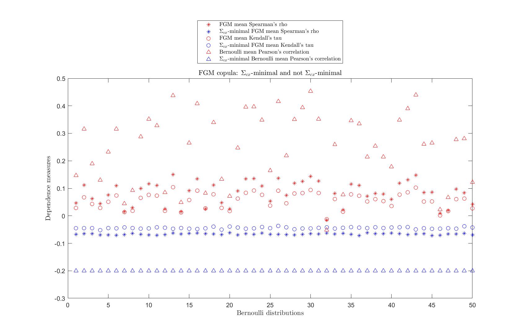
Figure 1: Dependence measures(mean Spearman’s rho and mean Kendall’s tau) of FGM corresponding to $\Sigma_{cx}$-smallest Bernoulli distributions (in blue) and of FGM corresponding to Bernoulli distributions not $\Sigma_{cx}$-smallest (in red).

In order to make a preliminary analysis, we randomly select fifty $\Sigma_{cx}$-smallest Bernoulli distributions and fifty generic Bernoulli distributions, of dimension $d=5$. Then, following Equation (5.1), from each corresponding FGM uniform distribution, we simulate 10.000 random samples, in order to assess each mean Spearman’s rho and each mean Kendall’s tau. In Figure 1, we compare these dependence measures and we can see that the mean Spearman’s rho and the mean Kendall’s tau are minimal and constant - except for simulation error - for FMG copulas that corresponds to $\Sigma_{cx}$-smallest elements in $\mathcal{SB}_{d}$.

6 Conclusion

In this paper, we study the minimal risk and minimal dependence distributions in the class $\mathcal{SB}_{d}$ of multivariate symmetric Bernoulli distributions and in two classes of copulas: the FGM and the extremal mixture copulas. Our key finding is to characterize all the distributions with minimal convex sums in $\mathcal{SB}_{d}$. This result is achieved using the algebraic representation of this class, introduced for the more general class $\mathcal{F}_{d}(p)$ by [10]. The advantage of this representation is that we can find an analytical set of polynomials that generates the whole class $\mathcal{SB}_{d}$ and that encode statistical properties of the corresponding distributions. Working with polynomials proved to be easier than working with distributions.

FGM copulas and extremal mixture copulas can be built using multivariate symmetric Bernoulli distributions and inherit some of their dependence properties. Indeed, our findings in the class $\mathcal{SB}_{d}$ allowed us to characterize the dependence properties of extremal mixture copulas corresponding to the minimal convex sums distributions in $\mathcal{SB}_{d}$. We also explicitly find the extremal $\Sigma$-countermonotonic copulas. Finally, we investigate the minimal dependence FGM copulas using some dependence measures.

Our future research has two main directions. The first direction is to further investigate the algebraic structure of multivariate Bernoulli distributions, that proved to be effective in studying dependence properties and bounds for aggregate risks. Our second research direction is to further investigate the connection between the dependence structure of symmetric Bernoulli distributions and their corresponding copulas. As an example, the characterization of the extremal negative dependence in the class of FGM copulas could be further investigated.

Appendix A Additional results the ideal $\mathcal{I}_{\mathcal{P}}$

The following results for the class $\mathcal{F}_{d}(p)$, where $p\in\mathbb{Q}$, are proved in [10]. Let let $p=s/t$ with $s\leq t$. We get $c={q}/{p}={(t-s)}/{s}$.

Proposition A.1.

The Gröbner basis of $\mathcal{I}_{\mathcal{P}}$ with respect to the lexicographic order is $GB=\{G_{i}(\boldsymbol{z})=(z_{i}-1)(z_{i}+c),G_{ik}(\boldsymbol{z})=1-z_{i}-z_{k}+z_{i}z_{k},i,k=,\ldots,2^{d-1},i<k\}$. A basis of the quotient space $\mathbb{Q}[z_{1},\ldots,z_{d-1}]/\mathcal{I}_{\mathcal{P}}$ is $\{1,z_{1},\ldots,z_{d-1}\}$.

If $p=\frac{1}{2}$ the Gröbner basis of $\mathcal{I}_{\mathcal{P}}$ with respect to the lexicographic order is $GB=\{G_{i}(\boldsymbol{z})=(z_{i}-1)(z_{i}+1),G_{ik}(\boldsymbol{z})=1-z_{i}-z_{k}+z_{i}z_{k},i,k=,\ldots,2^{d-1},i<k\}$.

We call the polynomials

$$F_{j_{1},\ldots,j_{n}}(\boldsymbol{z})=z_{j_{1}}\cdots z_{j_{n}}-\sum_{i=1}^{n}z_{j_{i}}+n-1$$

fundamental polynomials of the ideal $\mathcal{I}_{\mathcal{P}}$. In particular we denote by $F_{n}(\boldsymbol{z})$ the fundamental polynomial $F_{n}(\boldsymbol{z}):=F_{1,\ldots,n}(\boldsymbol{z})$, $n=2,\ldots,d-1$.

Proposition A.2.

The polynomials $P_{f}(\boldsymbol{z})\in\mathcal{C}_{\mathcal{H}}$ are linear combinations of the fundamental polynomials.

References

• [1] P. Embrechts and G. Puccetti, “Bounds for functions of dependent risks,” Finance and Stochastics, vol. 10, pp. 341–352, 2006.
• [2] M. Denuit, C. Genest, and É. Marceau, “Stochastic bounds on sums of dependent risks,” Insurance: Mathematics and Economics, vol. 25, no. 1, pp. 85–104, 1999.
• [3] G. Puccetti and L. Rüschendorf, “Sharp bounds for sums of dependent risks,” Journal of Applied Probability, vol. 50, no. 1, pp. 42–53, 2013.
• [4] R. Wang, L. Peng, and J. Yang, “Bounds for the sum of dependent risks and worst value-at-risk with monotone marginal densities,” Finance and Stochastics, vol. 17, pp. 395–417, 2013.
• [5] R. Kaas, J. Dhaene, and M. J. Goovaerts, “Upper and lower bounds for sums of random variables,” Insurance: Mathematics and Economics, vol. 27, no. 2, pp. 151–168, 2000.
• [6] H. Joe, Multivariate models and multivariate dependence concepts. CRC press, 1997.
• [7] G. Puccetti and R. Wang, “Extremal Dependence Concepts,” Statistical Science, vol. 30, no. 4, pp. 485 – 517, 2015.
• [8] R. B. Nelsen, An introduction to copulas. Springer, 2006.
• [9] E. Frostig, “Comparison of portfolios which depend on multivariate bernoulli random variables with fixed marginals,” Insurance: Mathematics and Economics, vol. 29, no. 3, pp. 319–331, 2001.
• [10] R. Fontana and P. Semeraro, “High dimensional bernoulli distributions: algebraic representation and applications,” Bernoulli, forthcoming. arXiv preprint arXiv:2205.12744, 2022.
• [11] W. Lee, K. C. Cheung, and J. Y. Ahn, “Multivariate countermonotonicity and the minimal copulas,” Journal of Computational and Applied Mathematics, vol. 317, pp. 589–602, 2017.
• [12] J. Dhaene and M. Denuit, “The safest dependence structure among risks,” Insurance: Mathematics and Economics, vol. 25, no. 1, pp. 11–21, 1999.
• [13] W. Lee and J. Y. Ahn, “On the multidimensional extension of countermonotonicity and its applications,” Insurance: Mathematics and Economics, vol. 56, pp. 68–79, 2014.
• [14] P. Embrechts, A. Höing, and A. Juri, “Using copulae to bound the value-at-risk for functions of dependent risks,” Finance and Stochastics, vol. 7, pp. 145–167, 2003.
• [15] A. J. McNeil, J. G. Nešlehová, and A. D. Smith, “On attainability of kendall’s tau matrices and concordance signatures,” Journal of Multivariate Analysis, vol. 191, p. 105033, 2022.
• [16] C. Blier-Wong, H. Cossette, and E. Marceau, “Stochastic representation of fgm copulas using multivariate bernoulli random variables,” Computational Statistics & Data Analysis, vol. 173, p. 107506, 2022.
• [17] R. Fontana and P. Semeraro, “Representation of multivariate bernoulli distributions with a given set of specified moments,” Journal of Multivariate Analysis, vol. 168, pp. 290–303, 2018.
• [18] R. Fontana, E. Luciano, and P. Semeraro, “Model risk in credit risk,” Mathematical Finance, vol. 31, no. 1, pp. 176–202, 2021.
• [19] G. M. Marchetti and N. Wermuth, “Palindromic bernoulli distributions,” Electronic Journal of Statistics, vol. 10, no. 2, pp. 2435 – 2460, 2016.
• [20] M. Terzer, Large scale methods to enumerate extreme rays and elementary modes. PhD thesis, ETH Zurich, 2009.
• [21] M. Sklar, “Fonctions de répartition à n dimensions et leurs marges,” in Annales de l’ISUP, vol. 8, pp. 229–231, 1959.
• [22] M. Shaked and J. G. Shanthikumar, Stochastic orders. Springer, 2007.
• [23] S. Cambanis, “Some properties and generalizations of multivariate eyraud-gumbel-morgenstern distributions,” Journal of Multivariate Analysis, vol. 7, no. 4, pp. 551–559, 1977.
• [24] C. Blier-Wong, H. Cossette, and E. Marceau, “Exchangeable fgm copulas,” arXiv preprint arXiv:2205.11302, 2022.
• [25] I. Gijbels, V. Kika, and M. Omelka, “On the specification of multivariate association measures and their behaviour with increasing dimension,” Journal of Multivariate Analysis, vol. 182, p. 104704, 2021.