See Beyond Seeing: Robust 3D Object Detection from Point Clouds
via Cross-Modal Hallucination
Abstract
This paper presents a novel framework for robust 3D object detection from point clouds via cross-modal hallucination. Our proposed approach is agnostic to either hallucination direction between LiDAR and 4D radar. We introduce multiple alignments on both spatial and feature levels to achieve simultaneous backbone refinement and hallucination generation. Specifically, spatial alignment is proposed to deal with the geometry discrepancy for better instance matching between LiDAR and radar. The feature alignment step further bridges the intrinsic attribute gap between the sensing modalities and stabilizes the training. The trained object detection models can deal with difficult detection cases better, even though only single-modal data is used as the input during the inference stage. Extensive experiments on the View-of-Delft (VoD) dataset show that our proposed method outperforms the state-of-the-art (SOTA) methods for both radar and LiDAR object detection while maintaining competitive efficiency in runtime.
I Introduction
Robust recognition and localization of objects in 3D space is a fundamental computer vision task and an essential capability for intelligent systems. In the context of autonomous driving, accurate 3D object detection is vital for safe motion planning, especially in a complex urban environment. Due to accurate depth measurement in long-range and robustness to illumination conditions, ranging sensors such as LiDAR and radar have attracted increasing attention recently and in turn, make the point clouds from them one of the most commonly used data representations for 3D object detection.
Despite advancements in LiDAR-based [1, 2, 3, 4, 5, 6, 7, 8, 9, 10] and radar-based 3D object detection [11, 12], each exhibits inherent drawbacks. LiDAR excels at producing dense point clouds but lacks per-point semantic information. Even though some LiDAR sensors can output point-level intensity values [13, 14], they are often inconsistent across semantic labels as lidar intensity is complexly determined by the distances between objects and LiDAR, rather than the object type alone [15]. Conversely, the emerging 4D radars, while prone to sparse data, present valuable semantic information per point, such as the Radar Cross Section (RCS) and Doppler velocity. Unlike LiDAR intensity, RCS is a distance-independent measurement uniquely determined by the object material and reflection angle. The Doppler velocity measures the moving speed of a detected point relative to the ego vehicle. Benefiting from the rich semantic information, fairly reasonable 3D object performance can be achieved using 4D radars in complex urban environments [12], even if some objects have less than 10 radar points.
Given the complementary nature of these sensors, we explore if one can assimilate the characteristics of the other while enhancing independent detection capacities. Indeed, due to the cost consideration, many low-end vehicles are only equipped with either radars or LiDARs. It is thus valuable to train a single-modal detection model from the multimodal data collected by some pilot vehicles equipped with both sensors, yet dispatch the trained models on low-end vehicles equipped with only one of them. Addressing this necessitates delving into cross-modal learning. Prior arts achieve this via either hallucination for feature augmentation [16, 17, 18, 19, 20] or knowledge distillation for backbone refinement [21, 22, 23, 24]. However, the learning direction in these prior works is unidirectional passing from the strong modality to the weak modality (e.g., RGB camera depth camera), insufficient to meet our goal.
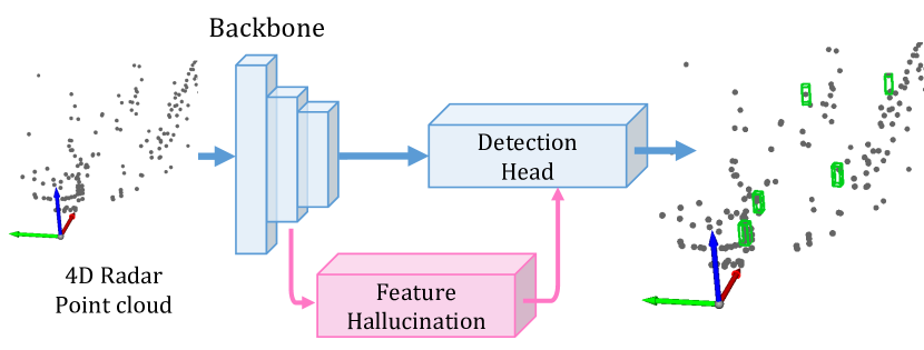
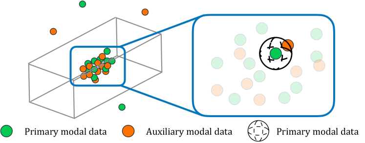
Unlike prior arts, in this work, we aim to realize a new cross-modal hallucination framework that can work in agnostic learning directions (i.e., LiDAR radar). To bridge the intrinsic sensing gap between two modalities, we introduce a novel selective matching module to enable feature-level alignment in the shared latent space. Our design enhances intra-modality features through cross-modal learning and supplements inter-modality features for improved detection robustness (see Fig. 1). Our method outperforms previous state-of-the-art (SOTA) methods in 3D object detection, which we demonstrate on the public View-of-Delft dataset in both LiDAR and radar object detection tasks. Our code will be publicly released upon acceptance.

II Related work
LiDAR object detection. LiDAR 3D object detection is categorized into voxel-based, point-based, and point-voxel approaches. Voxel-based methods transform point cloud data into grid cells, suitable for convolution operations [25, 26, 9, 1]. For example, [1] converts point clouds into 2D pseudo-images for faster inference, while [9] adopts a two-stage process, improving detection at a higher memory cost. Point-based techniques directly process unstructured point cloud data, minimizing data loss [2, 8, 7, 27]. Models in this category, such as [2, 7], utilize methodologies from [28] and [29] to extract features. Recent research introduces point-voxel networks that combine the best of both methods for enhanced accuracy [5, 3, 10, 30]. As highlighted by [7], these networks, like [5], perform well on the KITTI dataset [13], though they require more computation resources.
Radar object detection. Early efforts in radar-based object detection focused on 2D object detection [31, 32, 33]. It is only with the recent availability of 4D radar sensors that radar 3D object detection began receiving attention from researchers. [11] is an anchor-based 3D detection framework with a PointNet style backbone. It was only evaluated on short-range radar point clouds within 10 meters in front of the ego-vehicle, which is far too close for real-world autonomous scenarios. On the other hand, authors of the recently published dataset [12] successfully repurposed PointPillars [1] on radar point clouds. Although the 3D object detection architecture was designed for LiDAR point clouds, it achieved SOTA performance on their radar 3D object detection benchmark [12].
Cross-modal feature augmentation. Learning with side information involves using supplementary data during training to enhance single-modality networks [17, 19, 20, 16, 18, 22, 23, 21]. [18] pioneered using cross-modal hallucination in object detection by enhancing RGB image detection using depth image features. [16] integrated thermal data for RGB pedestrian detection. Recent works, like [21], utilize multi-modal features via knowledge distillation to improve 3D detection. However, many of these methods do not maximize cross-modal information use. For instance, [16, 18] require an extra backbone for hallucination instead of optimizing the original. Knowledge distillation techniques [22, 23, 21], while strengthening the backbone, overlook the potential of hallucinated data.
III Method
The proposed method is depicted in Fig. 2. Our framework includes (i) a point-based backbone for feature extraction, (ii) an instance feature aggregation module for aligning input modalities, (iii) a hallucination branch for cross-modal feature alignment, and (iv) a detection head for bounding box prediction. The selective matching module and shared detection head are training-specific. We use ‘primary’ and ‘auxiliary’ interchangeably to denote our two sensor modalities for clarity. At a high-level summary of our method, a backbone network takes point set of the primary modality and outputs a subset for the sampled foreground points with extracted features. For the auxiliary-modal data, we use a hat notation, such as . The instance feature aggregation module processes to obtain ‘centered points’ , adjusting point positions with a spatial offset . Features from both modalities are then aligned via non-linear mapping for hallucination, constrained by instance location, resulting in hallucination features . These are then concatenated with and fed into the detection head for final object recognition.
III-A Backbone Network
We construct our backbone network based on the Set-Abstraction (SA) layer proposed in PointNet++ [29] for better efficiency and to avoid information loss [8, 7]. Additionally, the farthest-point sampling (FPS) operation in SA layer is replaced with center-aware sampling proposed in [7] for better performance, which selects top- points based on the predicted centeredness. This predicted centeredness is constrained during training as:
|
|
(1) |
with as the ground truth centeredness and as network estimated value. is the corresponding mask value for each point proposed in [8], which assigns higher weights to points closer to the centroid of objects, and no weight at all for background points. The output of the backbone is denoted as with points and .
III-B Instance Feature Aggregation
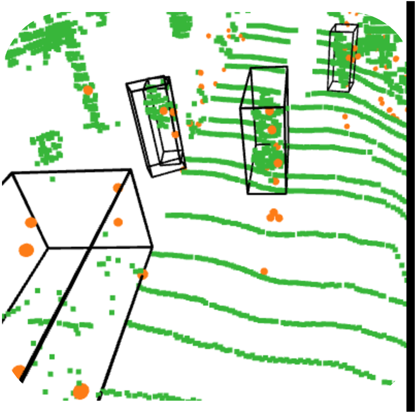
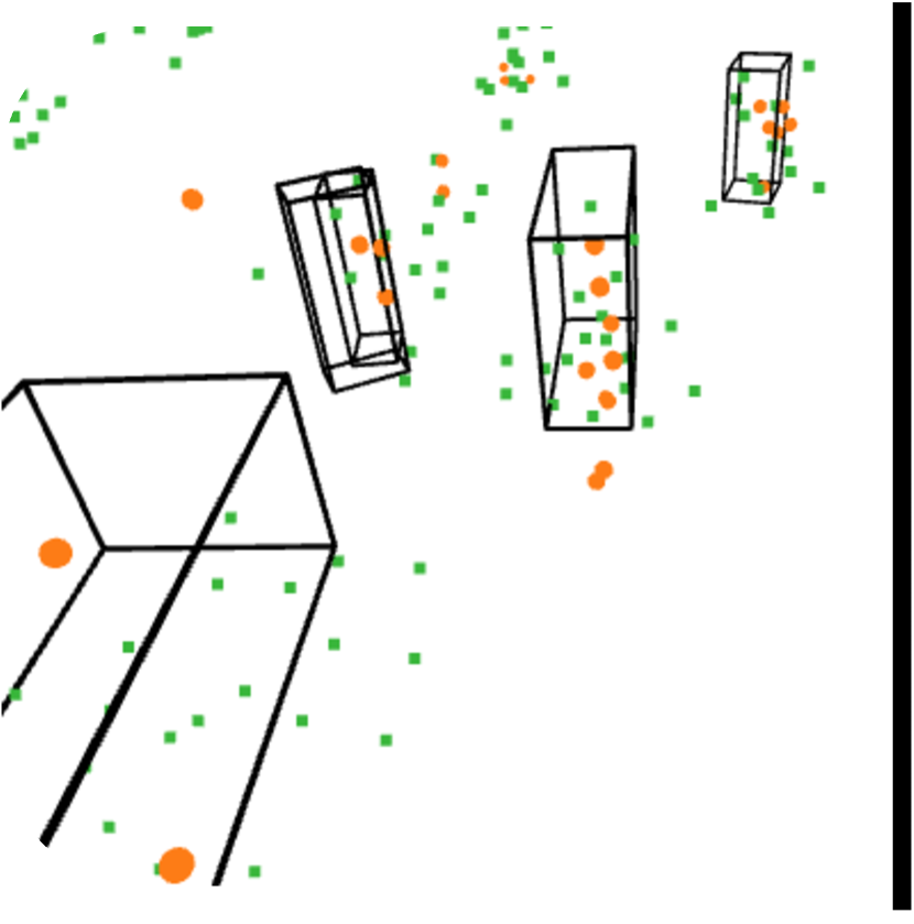
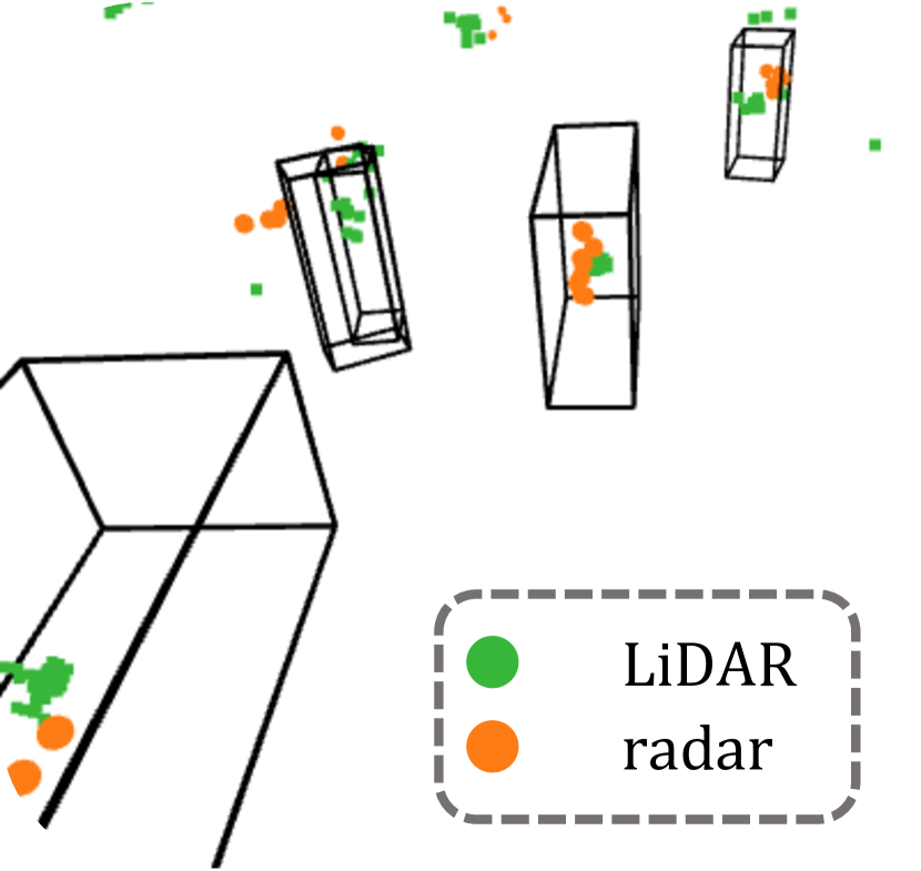
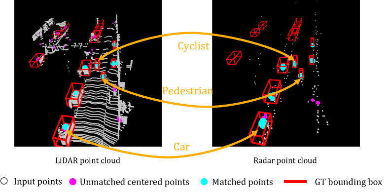
Single-stage detectors face challenges in point matching across different sensor modalities due to discrepancies between point clouds from co-located LiDAR and radar, evident in Fig.3(a). This difference, arising from fundamental sensor characteristics and unsolvable by calibration, is worsened by sampling randomness, especially in the backbone’s foreground sampling (c.f. Fig. 3(b)). To mitigate this, we use instance feature aggregation for improved alignment before cross-modal matching. This process is illustrated in Fig. 3(c). Following [34], we generate ‘centered points’ for context. Each foreground point, , gets an offset, , guiding it towards its object center. We constrain this regression process with a smooth-L1 loss as:
| (2) |
here is the true offset, and checks if is within an object. Points after this instance-aggregation step is denoted as , with each having a new position . Since points now cluster near the instance centroid, the subsequent SA layer’s ball query often groups the same points, resulting in almost identical instance features after max pooling. Thus, we can quickly establish instance matches between modalities by matching points in close spatial locations.
III-C Cross-Modal Feature Hallucination
Different sensing principles make LiDAR and radar instance features modality-specific. For instance, radar measures relative Doppler velocity [35, 36, 14], while LiDAR provides detailed object geometry. Given these intrinsic differences, it’s impractical to directly match all features across modalities. A solution is to ground cross-modal learning in a shared subspace, focusing on a subset of their features (the magenta block in Fig. 2). This mandates a feature projection module, allowing feature embedding in a shared latent space for both modalities. Specifically, given the instance-aggregated point set of the primary modality in the domain and clustered point set of the auxiliary modality in domain , we have two mapping functions acting as the feature projection: and to project both modalities to a shared common space. We adpot the MLP block for each of the mapping functions which yields two hallucination feature sets and respectively. The dimension of the shared common subspace, , is set empirically.
III-D Selective Matching
Using the projected hallucination features, we must match pairs between modalities for training, as shown by the purple block in Fig.2. As we note that noisy and incorrectly classified points tend to cluster at random spots, our approach involves a cross-modal Nearest Neighbor (1-NN) search within a specific radius to pinpoint the right matches, as shown in Fig. 4(a). Notice that only foreground points successfully shifted towards object centers can reach neighbor points from the other modality, as they are close in space. This proximity not only aids in efficient cross-modal representation learning but also reduces distractions from noisy data points. The cross-modal hallucination loss is as follows:
| (3) |
where is a binary matrix, and when and are a selected matching pair, otherwise . denotes the total number of matched pairs.
III-E Detection Head
Following [8, 7], we encode bounding boxes as multidimensional vectors comprising locations, scale, and orientation. The detection head, shown as the blue block in Fig. 2, has branches for confidence prediction and box refinement. The detection head’s loss function is:
| (4) |
To avoid trival solution for feature matching in Eq. 3, we use an extra detection head specifically for the shared space features, called shared detection head (the orange block in Fig. 2). This loss term is denoted as .
III-F Training and Inference
We adopt a two-step training strategy for stability. Unlike other methods [17, 16], our hallucination branch is co-optimized with the backbone in the second phase. In the first step, we train a basic detection network (shown by the green line in Fig.2) with loss:
| (5) |
In the second step, parameters from the first phase initialize the backbone and feature aggregation module. While the auxiliary backbone remains static, the primary one undergoes joint refinement with the hallucination module. A new detection head addresses the augmented feature space (represented by the orange line in Fig.2). The associated loss is:
| (6) |
When it comes to inference, only the primary modality data is applied, as shown by the blue line in Fig. 2.
IV Evaluation
IV-A Experimental Setup
Dataset. The View-of-Delft (VoD) dataset [12] offers calibrated, synchronized data from LiDAR, RGB camera, and 4D radar for 3D object detection, comprising 8693 frames captured in Delft’s urban environment. Unique to VoD is its inclusion of vulnerable road users like pedestrians and cyclists. Notably, VoD alone provides public access to simultaneous 4D radar recordings and LiDAR data and is thus selected for evaluation. While datasets such as nuScenes [14] have both radar and LiDAR data, their radars only offer 2D spatial measurements, limiting them for 3D object detection.
Implementation details. We follow the design of the backbone network in [7], which comprises several SA layers with center-aware sampling to remove noisy points. Next, the Vote Layer predicts an offset for each point to concentrate them on the corresponding object center for spatial alignment in centroid generation. After that, another SA layer is employed to aggregate instance-level features. Once we obtain point clusters for different objects, we project instance-level features to a shared subspace using a 4-layer MLP. These projected features are later concatenated back to the instance-level features for bounding box classification and regression. We use and in Eqn. 6 for all our experiments. Only the primary modal data will be used during inference. The best LiDAR and radar detection models are selected based on the best validation result for their respective detection tasks.
rowsep=1pt,colsep=2pt Method Type Car Pedestrian Cyclist mAP (IoU = 0.5) (IoU = 0.25) (IoU = 0.25) PointPillars†[1] V 35.90 34.90 43.10 38.00 SECOND[26] 35.07 25.47 33.82 31.45 CenterPoint[9] 32.32 17.37 40.25 29.98 PV-RCNN[5] PV 38.30 30.79 46.58 38.56 PointRCNN[2] P 15.99 34.01 26.50 25.50 3DSSD[8] 23.86 9.09 32.20 21.71 IASSD[7] 31.33 23.61 49.58 34.84 Ours 32.32 42.49 50.49 41.77
rowsep=1pt,colsep=2pt Method Type Car Pedestrian Cyclist mAP (IoU = 0.5) (IoU = 0.25) (IoU = 0.25) PointPillars†[1] V 75.60 55.10 55.40 62.10 SECOND[26] 77.69 59.95 65.50 67.71 CenterPoint[9] 68.29 66.90 64.42 66.54 PV-RCNN[5] PV 75.16 65.24 66.09 68.83 PointRCNN[2] P 61.51 67.36 67.03 65.30 3DSSD[8] 77.34 12.64 37.68 42.55 IASSD[7] 77.29 32.18 57.11 55.53 Ours 79.74 60.58 68.52 69.62
IV-B Overall Results
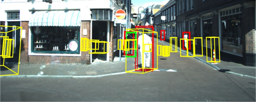
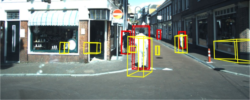
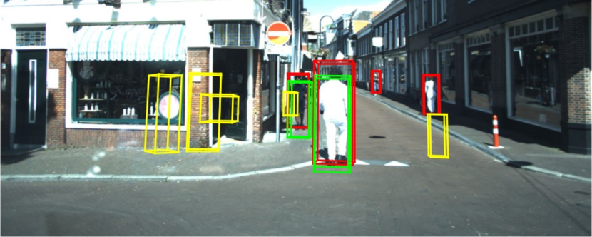
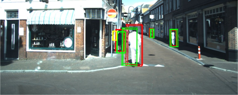
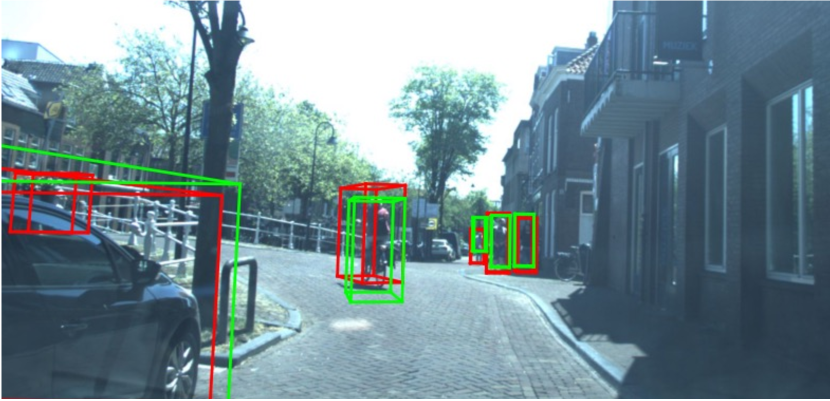
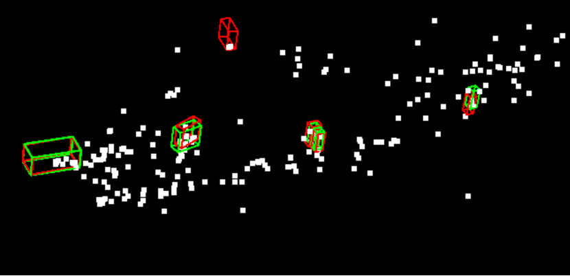
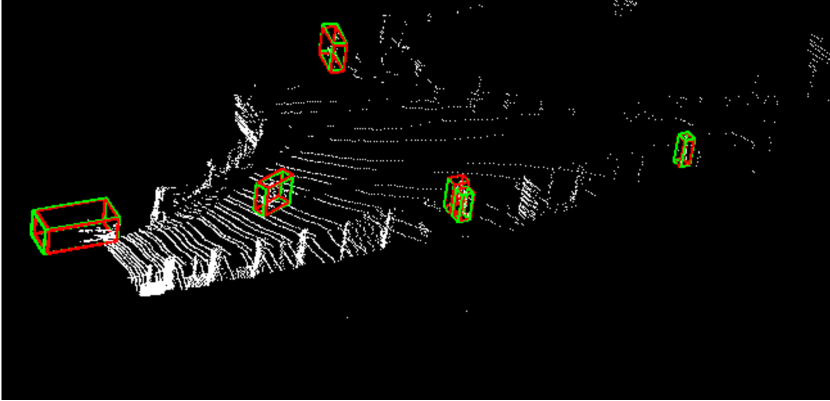
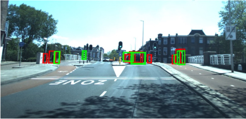
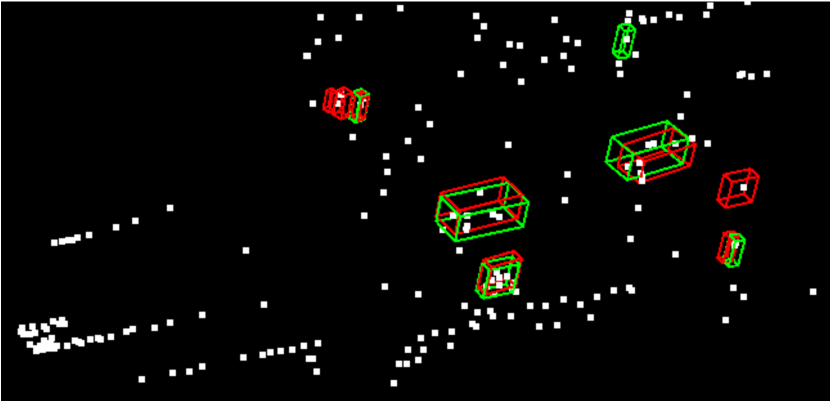
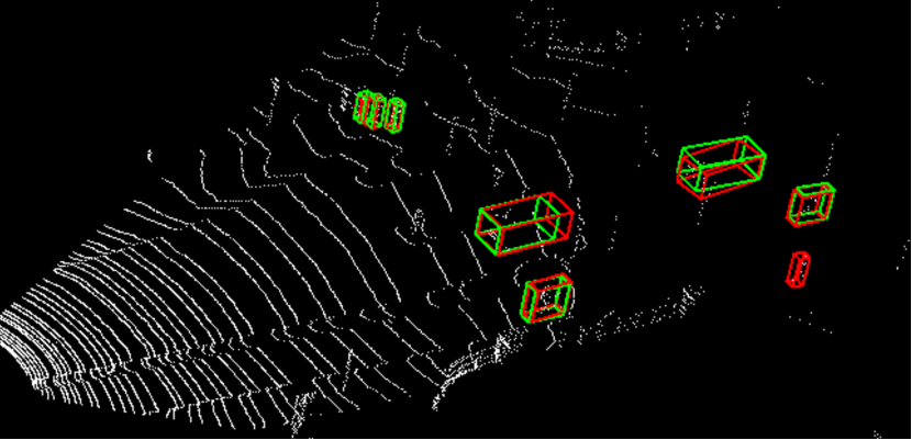
Tab. I and Tab. II show that our proposed framework gives rise to the best overall performance for both modalities, achieving mAP and mAP for radar and LiDAR object detection, respectively. Fig. 5 illustrates the qualitative results of our method.
Radar Object Detection. Despite the challenges of sparse and noisy radar point clouds, our detection method significantly outperforms SOTA techniques. PV-RCNN [5] excels in car detection due to reduced size ambiguity in voxel representation on sparse radar clouds. Yet, our method excels in detecting smaller objects like cyclists and pedestrians. Specifically, our model scores 42.49 mAP for pedestrians, outpacing the PV-RCNN by roughly 21.7%. This suggests that better representation for small objects with sparse clouds can be gleaned from cross-modal data, especially LiDAR. With our hallucination branch detailed in Sec. III-C, we encourage the radar detection network to emulate LiDAR’s instance representation, and our results affirm its efficacy.
LiDAR Object Detection. In LiDAR detection, our technique leads in car and cyclist categories, surpassing the runner-up by 2.6% and 2.2% mAP respectively. This boost stems from the Radar Cross Section (RCS) features’ semantic cues, distinguishing between metal and human skin[37, 38]. While two-stage detectors, such as [9, 5, 2], often excel in pedestrian detection through second-stage ROI refinement, they come with larger memory and slower speeds.
IV-C Ablation Study
To be consistent with LiDAR detection work, the more demanding 3D IoU in KITTI [13] with 0.7, 0.5, and 0.5 is used for LiDAR evaluation and 0.5, 0.25, 0.25 for radar evaluation on the VoD [12] validation set.
Effect of auxiliary-modal attributes. Through experiments with different auxiliary modal data inputs, we assess their influence on radar object detection using cross-modal supervision. Tab. III shows that radar detection improves when incorporating the LiDAR point cloud’s geometric information (, , ). The LiDAR intensity attribute has a slight impact, given radar’s stable semantic cues from RCS measurements. The Car category’s modest performance gain is due to around 25% of cars lacking radar points, hindering detection. Moreover, cars’ larger size versus cyclists and pedestrians complicates bounding box estimation with few points.
rowsep=1pt,colsep=2pt Auxiliary LiDAR Car Pedestrian Cyclist mAP point attributes (IoU=0.5) (IoU=0.25) (IoU=0.25) + none (baseline) 31.24 32.50 60.69 41.48 + 31.32 40.04 67.78 46.38 + 32.20 40.42 68.67 47.03
Effect of joint optimization. We study the effectiveness of our joint optimization strategy.
(a). Setup. We use the base network trained without cross-modal supervision and the hallucination branch as the ablation baseline. Later, we remove the hallucination branch of our framework shown in Fig. 2, freeze the backbone weights, and train a new detection head for performance comparison.
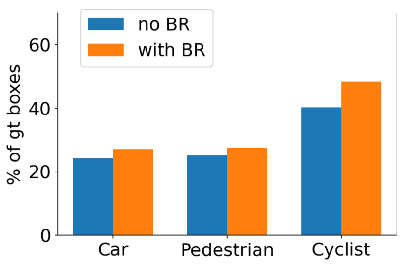
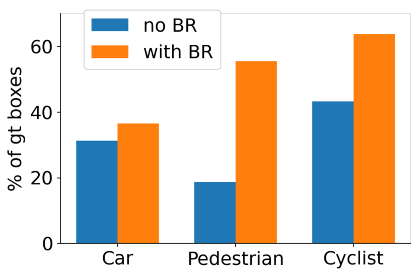
(b). Results. Looking at the first two rows in Tab. IV, mAP increases in both modalities, even without the hallucination branch. Significant improvements are seen with the Cyclist on radar and Pedestrian on LiDAR. For LiDAR, fewer car matches might cause a minor decline with only BR (Backbone Refinement), but other categories enhance. To understand why only refined backbone improves performance, we collected backbone output statistics. We can see from Fig. 6 that the percentage of instances containing more than five points gets improved. We propose that cross-modal representation learning enhances the backbone network’s feature extraction. These robust features are partially propagated to close points via max pooling, retaining more significant instance points in the final sampling layer, thus creating a robust instance feature representation for improved detection. Furthermore, the last row in each modality shows that the entire network with the hallucination branch leads to the best performance for all three categories, indicating its effectiveness and that extra cross-modal features can be encoded in our model for better detection inference.
rowsep=1pt,colsep=2pt Modality BR HA Car Pedestrian Cyclist mAP (IoU=0.5) (IoU = 0.25) (IoU = 0.25) radar 31.24 32.50 60.69 41.48 31.51 33.48 67.19 43.94 32.20 40.42 68.67 47.03 (IoU=0.7) (IoU = 0.5) (IoU = 0.5) mAP LiDAR 57.94 29.40 68.26 51.87 55.72 48.64 76.22 60.20 58.82 56.29 78.17 64.42
Effect of two-level alignment. We next study the LiDAR object detection results to better understand the influence of our alignment strategies introduced in Sec. III-B and Sec. III-C. Tab. V shows that spatial alignment in centroid generation is the key to cross-modal learning. When removed, the discrepancy between modalities results in mismatching pairs. Misleading supervision signals caused by mismatched pairs degenerate the network performance, especially for large objects like Cars. When the spatial alignment in centroid generation is added, the model establishes correct cross-modal instance matches and improves mAP, as shown in the third row of Tab. V. We attribute the slight performance drops on cars to fewer matched instances in this category. As expected, the feature alignment will only function and positively contribute to the model when the cross-modal points are spatially aligned first. The last row shows that combining two alignment operations yields the best performance. Similar conclusions are observed for radar detection, and we omit its discussion to avoid repetition.
rowsep=1pt,colsep=2pt Modality Spatial Feature Car Pedestrian Cyclist mAP (IoU=0.7) (IoU=0.5) (IoU=0.5) LiDAR 57.94 29.40 68.26 51.87 28.88 30.22 64.33 41.15 57.29 48.66 77.70 61.22 58.82 56.29 78.17 64.42
IV-D Runtime Efficiency
rowsep=1pt,colsep=2pt Type Method Memory Parallel Speed Voxel-based PointPillars[1] 354MB 69 123 SECOND[26] 710MB 34 34 Point-Voxel PV-RCNN[5] 1223MB 17 13 Point-based pointRCNN[2] 560MB 43 14 3DSSD[8] 502MB 48 20 IA-SSD[7] 120MB 202 23 Ours 133MB 183 23
We evaluate the memory consumption and inference speed compared with SOTA methods with LiDAR as the primary modal input. As shown in Tab. VI, our method has the second lowest memory footprint among all methods and the fastest inference speed in the point-based methods. Together with Tab. II and Tab. I, our framework has the best balance between efficiency and accuracy.
V Conclusions and Future Work
This work introduced a novel framework to improve the robustness of single-modal 3D object detection via cross-modal supervision. Our method is able to effectively exploit the side information from auxiliary modality data for a better-informed backbone network and a robust hallucination branch. Bespoken spatial and domain alignment strategies are also proposed to address the fundamental discrepancy across modalities and showed a significant performance improvement. Experimental results on VoD[12] demonstrate that our method outperforms SOTA methods in object detection for both radar and LiDAR while maintaining a competitive memory footprint and runtime efficiency.
References
- [1] A. H. Lang, S. Vora, H. Caesar, L. Zhou, J. Yang, and O. Beijbom, “Pointpillars: Fast encoders for object detection from point clouds,” in Proceedings of the IEEE/CVF conference on computer vision and pattern recognition, 2019, pp. 12 697–12 705.
- [2] S. Shi, X. Wang, and H. Li, “Pointrcnn: 3d object proposal generation and detection from point cloud,” in Proceedings of the IEEE/CVF conference on computer vision and pattern recognition, 2019, pp. 770–779.
- [3] Z. Yang, Y. Sun, S. Liu, X. Shen, and J. Jia, “Std: Sparse-to-dense 3d object detector for point cloud,” in Proceedings of the IEEE/CVF international conference on computer vision, 2019, pp. 1951–1960.
- [4] Z. Liu, X. Zhao, T. Huang, R. Hu, Y. Zhou, and X. Bai, “Tanet: Robust 3d object detection from point clouds with triple attention,” Proceedings of the AAAI Conference on Artificial Intelligence, vol. 34, no. 07, pp. 11 677–11 684, Apr. 2020. [Online]. Available: https://ojs.aaai.org/index.php/AAAI/article/view/6837
- [5] S. Shi, C. Guo, L. Jiang, Z. Wang, J. Shi, X. Wang, and H. Li, “Pv-rcnn: Point-voxel feature set abstraction for 3d object detection,” in Proceedings of the IEEE/CVF Conference on Computer Vision and Pattern Recognition, 2020, pp. 10 529–10 538.
- [6] S. Shi, Z. Wang, J. Shi, X. Wang, and H. Li, “From points to parts: 3d object detection from point cloud with part-aware and part-aggregation network,” IEEE transactions on pattern analysis and machine intelligence, vol. 43, no. 8, pp. 2647–2664, 2020.
- [7] Y. Zhang, Q. Hu, G. Xu, Y. Ma, J. Wan, and Y. Guo, “Not all points are equal: Learning highly efficient point-based detectors for 3d lidar point clouds,” in Proceedings of the IEEE/CVF Conference on Computer Vision and Pattern Recognition, 2022, pp. 18 953–18 962.
- [8] Z. Yang, Y. Sun, S. Liu, and J. Jia, “3dssd: Point-based 3d single stage object detector,” in Proceedings of the IEEE/CVF conference on computer vision and pattern recognition, 2020, pp. 11 040–11 048.
- [9] T. Yin, X. Zhou, and P. Krahenbuhl, “Center-based 3d object detection and tracking,” in Proceedings of the IEEE/CVF conference on computer vision and pattern recognition, 2021, pp. 11 784–11 793.
- [10] J. Noh, S. Lee, and B. Ham, “Hvpr: Hybrid voxel-point representation for single-stage 3d object detection,” in Proceedings of the IEEE/CVF Conference on Computer Vision and Pattern Recognition, 2021, pp. 14 605–14 614.
- [11] K. Bansal, K. Rungta, S. Zhu, and D. Bharadia, “Pointillism: Accurate 3d bounding box estimation with multi-radars,” in Proceedings of the 18th Conference on Embedded Networked Sensor Systems, 2020, pp. 340–353.
- [12] A. Palffy, E. Pool, S. Baratam, J. F. Kooij, and D. M. Gavrila, “Multi-class road user detection with 3+ 1d radar in the view-of-delft dataset,” IEEE Robotics and Automation Letters, vol. 7, no. 2, pp. 4961–4968, 2022.
- [13] A. Geiger, P. Lenz, and R. Urtasun, “Are we ready for autonomous driving? the kitti vision benchmark suite,” in 2012 IEEE Conference on Computer Vision and Pattern Recognition, 2012, pp. 3354–3361.
- [14] H. Caesar, V. Bankiti, A. H. Lang, S. Vora, V. E. Liong, Q. Xu, A. Krishnan, Y. Pan, G. Baldan, and O. Beijbom, “nuscenes: A multimodal dataset for autonomous driving,” in Proceedings of the IEEE/CVF conference on computer vision and pattern recognition, 2020, pp. 11 621–11 631.
- [15] P. Chazette, J. Totems, L. Hespel, and J.-S. Bailly, “5 - principle and physics of the lidar measurement,” in Optical Remote Sensing of Land Surface, N. Baghdadi and M. Zribi, Eds. Elsevier, 2016, pp. 201–247. [Online]. Available: https://www.sciencedirect.com/science/article/pii/B9781785481024500053
- [16] D. Xu, W. Ouyang, E. Ricci, X. Wang, and N. Sebe, “Learning cross-modal deep representations for robust pedestrian detection,” in Proceedings of the IEEE conference on computer vision and pattern recognition, 2017, pp. 5363–5371.
- [17] M. R. U. Saputra, P. P. de Gusmao, C. X. Lu, Y. Almalioglu, S. Rosa, C. Chen, J. Wahlström, W. Wang, A. Markham, and N. Trigoni, “Deeptio: A deep thermal-inertial odometry with visual hallucination,” IEEE Robotics and Automation Letters, vol. 5, no. 2, pp. 1672–1679, 2020.
- [18] J. Hoffman, S. Gupta, and T. Darrell, “Learning with side information through modality hallucination,” in Proceedings of the IEEE conference on computer vision and pattern recognition, 2016, pp. 826–834.
- [19] J. Lezama, Q. Qiu, and G. Sapiro, “Not afraid of the dark: Nir-vis face recognition via cross-spectral hallucination and low-rank embedding,” in Proceedings of the IEEE conference on computer vision and pattern recognition, 2017, pp. 6628–6637.
- [20] C. Choi, S. Kim, and K. Ramani, “Learning hand articulations by hallucinating heat distribution,” in Proceedings of the IEEE International Conference on Computer Vision, 2017, pp. 3104–3113.
- [21] W. Zheng, M. Hong, L. Jiang, and C.-W. Fu, “Boosting 3d object detection by simulating multimodality on point clouds,” in Proceedings of the IEEE/CVF Conference on Computer Vision and Pattern Recognition, 2022, pp. 13 638–13 647.
- [22] Z. Yuan, X. Yan, Y. Liao, Y. Guo, G. Li, S. Cui, and Z. Li, “X-trans2cap: Cross-modal knowledge transfer using transformer for 3d dense captioning,” in Proceedings of the IEEE/CVF Conference on Computer Vision and Pattern Recognition, 2022, pp. 8563–8573.
- [23] S. Gupta, J. Hoffman, and J. Malik, “Cross modal distillation for supervision transfer,” in Proceedings of the IEEE conference on computer vision and pattern recognition, 2016, pp. 2827–2836.
- [24] S. Ren, Y. Du, J. Lv, G. Han, and S. He, “Learning from the master: Distilling cross-modal advanced knowledge for lip reading,” in Proceedings of the IEEE/CVF Conference on Computer Vision and Pattern Recognition, 2021, pp. 13 325–13 333.
- [25] Y. Zhou and O. Tuzel, “Voxelnet: End-to-end learning for point cloud based 3d object detection,” in Proceedings of the IEEE conference on computer vision and pattern recognition, 2018, pp. 4490–4499.
- [26] Y. Yan, Y. Mao, and B. Li, “Second: Sparsely embedded convolutional detection,” Sensors, vol. 18, no. 10, p. 3337, 2018.
- [27] W. Shi and R. Rajkumar, “Point-gnn: Graph neural network for 3d object detection in a point cloud,” in Proceedings of the IEEE/CVF conference on computer vision and pattern recognition, 2020, pp. 1711–1719.
- [28] C. R. Qi, H. Su, K. Mo, and L. J. Guibas, “Pointnet: Deep learning on point sets for 3d classification and segmentation,” in Proceedings of the IEEE conference on computer vision and pattern recognition, 2017, pp. 652–660.
- [29] C. R. Qi, L. Yi, H. Su, and L. J. Guibas, “Pointnet++: Deep hierarchical feature learning on point sets in a metric space,” Advances in neural information processing systems, vol. 30, 2017.
- [30] C. He, H. Zeng, J. Huang, X.-S. Hua, and L. Zhang, “Structure aware single-stage 3d object detection from point cloud,” in Proceedings of the IEEE/CVF conference on computer vision and pattern recognition, 2020, pp. 11 873–11 882.
- [31] Y. Wang, Z. Jiang, X. Gao, J.-N. Hwang, G. Xing, and H. Liu, “Rodnet: Radar object detection using cross-modal supervision,” in Proceedings of the IEEE/CVF Winter Conference on Applications of Computer Vision, 2021, pp. 504–513.
- [32] A. Zhang, F. E. Nowruzi, and R. Laganiere, “Raddet: Range-azimuth-doppler based radar object detection for dynamic road users,” in 2021 18th Conference on Robots and Vision (CRV). IEEE, 2021, pp. 95–102.
- [33] K. Qian, S. Zhu, X. Zhang, and L. E. Li, “Robust multimodal vehicle detection in foggy weather using complementary lidar and radar signals,” in Proceedings of the IEEE/CVF Conference on Computer Vision and Pattern Recognition, 2021, pp. 444–453.
- [34] C. R. Qi, O. Litany, K. He, and L. J. Guibas, “Deep hough voting for 3d object detection in point clouds,” in Proceedings of the IEEE International Conference on Computer Vision, 2019.
- [35] M. Meyer and G. Kuschk, “Deep learning based 3d object detection for automotive radar and camera,” in 2019 16th European Radar Conference (EuRAD). IEEE, 2019, pp. 133–136.
- [36] ——, “Automotive radar dataset for deep learning based 3d object detection,” in 2019 16th European Radar Conference (EuRAD), 2019, pp. 129–132.
- [37] E. Bel Kamel, A. Peden, and P. Pajusco, “Rcs modeling and measurements for automotive radar applications in the w band,” in 2017 11th European Conference on Antennas and Propagation (EUCAP), 2017, pp. 2445–2449.
- [38] S. Lee, S. Kang, S.-C. Kim, and J.-E. Lee, “Radar cross section measurement with 77 ghz automotive fmcw radar,” in 2016 IEEE 27th Annual International Symposium on Personal, Indoor, and Mobile Radio Communications (PIMRC). IEEE, 2016, pp. 1–6.