Identifiability Study of Lithium-Ion Battery Capacity Fade Using Degradation Mode Sensitivity for a Minimally and Intuitively Parametrized Electrode-Specific Cell OCV Model

Abstract

When two electrode open-circuit potentials form a full-cell OCV (open-circuit voltage) model, cell-level SOH parameters related to LLI (loss of lithium inventory) and LAM (loss of active materials) naturally appear. Such models have been used to interpret experimental OCV measurements and infer these SOH parameters associated with capacity fade. In this work, we first propose a minimal and intuitive parametrization of the OCV model that involves pristine-condition-agnostic and cutoff-voltage-independent parameters such as the N/P ratio and Li/P ratio. We then study the modal identifiability of capacity fade by mathematically deriving the gradients of electrode slippage and cell OCV with respect to these SOH parameters, where the electrode differential voltage fractions, which characterize each electrode’s relative contribution to the OCV slope, play a key role in passing the influence of a fixed cutoff voltage to the parameter sensitivity. The sensitivity gradients of the total capacity also reveal four characteristic regimes regarding how much lithium inventory and active materials are limiting the apparent capacity. We show the usefulness of these sensitivity gradients with two applications regarding degradation mode identifiability from OCV measurements at different SOC windows and relations between incremental capacity fade and the underlying LLI and LAM rates.

[I2R] organization=Institute for Infocomm Research (I2R), Agency for Science, Technology and Research (A*STAR),addressline=1 Fusionopolis Way, #21-01 Connexis South, postcode=Singapore 138632, country=Republic of Singapore,

Proposed a minimal and intuitive parametrization of the electrode-specific OCV model.

Mathematically derived the gradients of electrode slippage and cell OCV w.r.t. parameters.

Introduced electrode differential voltage fractions coming from fixed cutoff-voltage effects.

Selected informative SOC windows for degradation mode estimation by Fisher information.

Related Coulombic efficiency and capacity retention to small LLI and LAM rates rigorously.

1 Introduction: Characterizing Degradation by SOH parameters

Lithium-ion batteries degrade over time upon operation and storage due to many complex and coupled physicochemical mechanisms and processes [1, 2]. Degradation causes a battery cell to lose capacity and rate capability, where the former represents charge throughput between the cell’s fully charged and discharged state, while the latter indicates the maximum charge/discharge C-rate the cell can withhold within a short period. These two aspects of aging are usually called capacity and power fade, respectively [3].

One technical subtlety here is that the fully charged and discharged state is defined by the cell OCV (open-circuit voltage) reaching a pre-specified upper and lower cutoff voltage $U_{\mathrm{max}}$ and $U_{\mathrm{min}}$, respectively, and the charge throughput between these two states is named the total capacity $\hat{Q}_{\mathrm{max}}$ and is what capacity fade specifically concerns [4]. However, under finite-current operation, the observed terminal voltage shall reach a cutoff voltage before the underlying OCV does due to polarization in non-equilibrium, so the commonly reported charge/discharge capacity during cycling can be significantly smaller than the total capacity, unless both charging and discharging have a trailing CV (constant-voltage) phase with a small enough cutoff current. The key is that the cell must have reached quasi-equilibrium at $U_{\mathrm{max}}$ and $U_{\mathrm{min}}$ before and after the Coulomb counting, respectively. The total capacity depends only on the thermodynamic properties of the cell, while the charge/discharge capacity also depends on the kinetic characteristics and operation protocols. Therefore, the latter’s reduction upon aging is due to both capacity and power fade. It is not uncommon to see a charge/discharge capacity being confused with the total capacity in literature, but the distinction is important for the various modes of capacity fade.

A battery cell’s voltage response to an input current profile can be captured and predicted by a cell model, be it physics-based and derived from first principles, or semi-empirical and approximated by an equivalent circuit [4]. Therefore, within such a model, a cell’s capacity and rate capability are completely encoded by certain model parameters, which we will refer to as SOH (state of health) parameters, and the granularity of this parametrization depends on the model’s complexity. Such SOH parameters interface between the underlying physicochemical degradation mechanisms and the apparent cell performance metrics, so the performance decay caused by the change of a particular parameter is also called a degradation mode [3]. If such SOH parameters can be identified from observed cell behaviors, we can track how they evolve across a cell’s lifetime under different operating conditions, which might provide valuable clues about dominant aging mechanisms, inspire the formulation of more accurate degradation models, enable more effective aging-aware battery management and control, and even guide battery design to attenuate degradation.

Although we treat SOH here as a loose term that denotes a cell’s capacity and rate capability, whose precise meaning depends on the context of a particular cell model, SOH historically often refers to the total capacity $\hat{Q}_{\mathrm{max}}$ and equivalent internal resistance $R_{0}$ of a cell [5], which form possibly the coarsest-grained description of capacity and power fade, and correspond to a simple ECM (equivalent circuit model) with only a monolithic OCV source $U_{\mathrm{OCV}}(z)$ assumed to be unchanged upon aging [6] and a series resistor of $R_{0}$. Here $z$ denotes the cell SOC (state of charge), whose precise meaning will be clarified later. There has been an enormous amount of research dedicated to estimating $\hat{Q}_{\mathrm{max}}$ and $R_{0}$ from voltage and current measurements [5, 7], but such parametrization is too coarse-grained to shed light on possible underlying degradation mechanisms. In this work, we will restrict ourselves to capacity fade only and focus on a natural refinement of the monolithic OCV relation by constructing the cell OCV as the difference between the PE (positive electrode/cathode) and NE (negative electrode/anode) OCP (open-circuit potential):

$$U_{\mathrm{OCV}}(z^{-},z^{+})=U^{+}_{\mathrm{OCP}}(z^{+})-U^{-}_{\mathrm{OCP}}(z^{-}),$$ (1)

where $z^{\pm}$ are the PE and NE SOC to be defined later, and three SOH parameters lithium inventory $\hat{Q}^{\mathrm{Li}}_{\mathrm{max}}$, PE active materials $\hat{Q}^{+}_{\mathrm{max}}$, and NE active materials $\hat{Q}^{-}_{\mathrm{max}}$, all measured in charges, will naturally surface in place of a single total capacity $\hat{Q}_{\mathrm{max}}$ as the SOH parameters, which correspond to the three well-known capacity fade modes: LLI (loss of lithium inventory), LAMp, and LAMn (loss of active materials in PE/NE), respectively [8].

The development history of the above electrode-specific OCV model, though with different parametrization, has recently been reviewed by Olson et al. [9] under the context of DV (differential voltage) and IC (incremental capacity) analysis. Indeed, this model was used to estimate the three modes of capacity fade first by DV [10] and IC [8] analysis. However, DV and IC analysis is not yet a fully automatic technique, and they require users to judge how the peaks and troughs of the full-cell DV and IC curves are associated with electrode OCP features [9]. Later, researchers attempted to estimate the three modes of LLI, LAMn, and LAMp directly by fitting the model OCV curve to experimental measurements using classical NLS (nonlinear least squares) [3, 11]. In particular, Birkl et al. [3] experimentally validate this approach by assembling coin cells with a controlled amount of lithium inventory and active materials, which serve as the ground truth against optimization results from NLS. However, they parametrize their electrode-specific OCV

$$U_{\mathrm{OCV}}(z)=U^{+}_{\mathrm{OCP}}(z^{+}_{\mathrm{max}}-z(z^{+}_{\mathrm{max}}-z^{+}_{\mathrm{min}}))-U^{-}_{\mathrm{OCP}}(z^{-}_{\mathrm{min}}+z(z^{-}_{\mathrm{max}}-z^{-}_{\mathrm{min}}))$$ (2)

by the extreme electrode SOC $z_{\mathrm{max}}^{\pm}$ and $z_{\mathrm{min}}^{\pm}$, which are constrained by the upper and lower cutoff voltage and have rather complicated dependence on the three modes. Mohtat et al. [11] instead use the OCV in terms of the discharge throughput $Q_{\mathrm{d}}$ counted from the fully charged state:

$$U_{\mathrm{OCV}}(Q_{\mathrm{d}})=U^{+}_{\mathrm{OCP}}(z^{+}_{\mathrm{min}}+Q_{\mathrm{d}}/\hat{Q}_{\mathrm{max}}^{+})-U^{-}_{\mathrm{OCP}}(z^{-}_{\mathrm{max}}-Q_{\mathrm{d}}/\hat{Q}_{\mathrm{max}}^{-}),$$ (3)

which is parametrized by $z^{+}_{\mathrm{min}}$, $z^{-}_{\mathrm{max}}$, and $\hat{Q}_{\mathrm{max}}^{\pm}$, subject to the constraint $U^{+}_{\mathrm{OCP}}(z^{+}_{\mathrm{min}})-U^{-}_{\mathrm{OCP}}(z^{-}_{\mathrm{max}})=U_{\mathrm{max}}$. They also derive the gradient of $U_{\mathrm{OCV}}(Q_{\mathrm{d}})$ with respect to the four parameters and use Fisher information to quantify the parametric identifiability. This OCV model has been incorporated in PyBaMM [12], an open battery modeling package implemented in Python, and much subsequent work on model-based degradation mode estimation has used different variants of this four-parameter formulation [13, 14].

In this work, we argue that the above parametrizations based on electrode SOC at a certain cutoff voltage involve non-independent parameters, of which the redundancy complicates their estimation. Moreover, the cutoff voltage is an operational parameter that is not intrinsic to the aging state of a cell, so a parametrization that depends on it blurs the intrinsic degradation trend and makes the SOH parameters less intuitive to interpret. We also argue not to parametrize the OCV directly by the LLI, LAMn and LAMp percentage [8, 9], as these quantities rely on specifying the pristine-cell SOH parameters, which are irrelevant to the current SOH and could be arbitrary.

We propose a parametrization that makes $U_{\mathrm{OCV}}(Q_{\mathrm{d}})$ depend only on three SOH parameters: lithium inventory $\hat{Q}^{\mathrm{Li}}_{\mathrm{max}}$, NE active materials $\hat{Q}^{-}_{\mathrm{max}}$, and PE active materials $\hat{Q}^{+}_{\mathrm{max}}$, all measured in equivalent charges, or equivalently by the Li/P (lithium-to-positive) ratio $z^{+}_{0}=\hat{Q}^{\mathrm{Li}}_{\mathrm{max}}/\hat{Q}^{+}_{\mathrm{max}}$, N/P (negative-to-positive) ratio $r_{\mathrm{N/P}}=\hat{Q}^{-}_{\mathrm{max}}/\hat{Q}^{+}_{\mathrm{max}}$, and $\hat{Q}^{+}_{\mathrm{max}}$. These parameters do not depend on any cutoff voltage or pristine-cell SOH, are independent, and their changes directly and intuitively capture the three modes of LLI, LAMn, and LAMp. Moreover, after the upper and lower cutoff voltage of a cell are specified to define the cell SOC $z$, the SOC-based OCV $U_{\mathrm{OCV}}(z)$ only depends on two independent dimensionless parameters of Li/P and N/P ratio. Along the way, we will also clarify several common misconceptions regarding the use of an electrode-specific OCV model.

We will further analytically derive the gradients of $U_{\mathrm{OCV}}(z)$, $U_{\mathrm{OCV}}(Q_{\mathrm{d}})$, and total capacity $\hat{Q}_{\mathrm{max}}$ with respect to the SOH parameters, and demonstrate the further insights provided by this sensitivity analysis beyond what has been shown in [11, 15]. In particular, we will introduce the electrode DV (differential voltage) fraction, which is instrumental in channeling the effects of a fixed upper and lower cutoff voltage into the sensitivity gradients. The analytic results will also be visualized, verified, and corroborated by simulations.

Finally, we will also present two applications of our analytic results. The first is on feeding the sensitivity gradients to the Fisher information matrix to quantify the identifiability of the Li/P and N/P ratio from measurements of $U_{\mathrm{OCV}}(z)$. The second application is on using the derived gradients for rigorous first-order analysis to relate the measurable Coulombic efficiency and capacity retention to the underlying LLI and LAM rates, which clarifies and generalizes the results in [16].

2 Methodology and Analysis

Before diving into the degradation mode parametrization and identifiability, we want to clarify a few concepts that could be ambiguous in literature.

2.1 Electrode OCP: Stoichiometry, Electrode SOC and Active Material Amount

For a lithium intercalation electrode, the stoichiometry $x$ is literally the stoichiometric coefficient of lithium in the active material chemical formula that indicates the lithiation state, usually with $0\leq x\leq 1$ such as in graphite $\mathrm{Li}_{x}\mathrm{C}_{6}$ and LFP (lithium iron phosphate) $\mathrm{Li}_{x}\mathrm{FePO}_{4}$, where $x=0$ and $x=1$ corresponds to the theoretical fully delithiated and lithiated state, respectively. The chemical formula also yields the theoretical electrode specific capacity, such as $q_{\mathrm{max}}^{-}=372\mathrm{mAh/g}$ for $\mathrm{Li}_{x}\mathrm{C}_{6}$ and $q_{\mathrm{max}}^{+}=170\mathrm{mAh/g}$ for $\mathrm{Li}_{x}\mathrm{FePO}_{4}$. In the following, we will use the superscript ⁺ and ^- to indicate quantities associated with PE and NE active materials, respectively.

An ideal open-circuit potential relation $U_{\mathrm{OCP}}^{\pm}(x^{\pm})$ is with respect to the stoichiometry $x^{\pm}$, where the potential is measured against the standard lithium metal electrode. However, due to material instability and electrochemical side reactions in practice, we cannot fully lithiate or delithiate an electrode. Besides, we also lack means to directly measure the electrode stoichiometry $x^{\pm}$, unless we start with a pristine electrode with a precisely known amount of active materials, which implies $x^{-}=0$ for NE materials like graphite or $x^{+}=1$ for PE materials like LFP initially, and we can use Coulomb counting and the active material mass to deduce subsequent lithiation states.

In most cases, we can only lithiate/delithiate an electrode (half cell) across a usable potential window and obtain $U_{\mathrm{OCP}}^{\pm}(Q^{\pm})$ from voltage measurements and Coulomb counting. We only know that the charge throughput $Q^{\pm}$ is linearly related to $x^{\pm}$, but we have no access to the slope and intercept. Hence, the best we can do is to define an electrode SOC $z^{\pm}\in[0,1]$ such that $z^{\pm}=0$ corresponds to some unknown $x_{\mathrm{min}}^{\pm}$ at the top of the usable potential window, while $z^{\pm}=1$ corresponds to some unknown $x_{\mathrm{max}}^{\pm}$ at the bottom. This way, we can map $Q^{\pm}$ linearly to $z^{\pm}$ and obtain the most commonly seen OCP relations $U_{\mathrm{OCP}}^{\pm}(z^{\pm})$.

The Coulomb counting also tells us the charge throughput associated with the whole interval of $0\leq z^{\pm}\leq 1$, which is the usable electrode capacity $\hat{Q}_{\mathrm{max}}^{\pm}$. Note that

$$\hat{Q}_{\mathrm{max}}^{\pm}=(x_{\mathrm{max}}^{\pm}-x_{\mathrm{min}}^{\pm})Q_{\mathrm{max}}^{\pm}$$ (4)

can be much smaller than the theoretical electrode capacity $Q_{\mathrm{max}}^{\pm}$ associated with $0\leq x^{\pm}\leq 1$, and without knowing the active material mass, we cannot obtain $Q_{\mathrm{max}}^{\pm}$. Moreover, since $z^{\pm}$ also relates linearly to $x^{\pm}$, we must have

$$z^{\pm}=\frac{x^{\pm}-x^{\pm}_{\mathrm{min}}}{x^{\pm}_{\mathrm{max}}-x^{\pm}_{\mathrm{min}}},$$ (5)

although we do not know these stoichiometry limits in general.

Note also that mathematically, the choice of this upper and lower cutoff potential for defining $z^{\pm}=0$ and $z^{\pm}=1$, respectively, is arbitrary, as long as $\hat{Q}_{\mathrm{max}}^{\pm}$ is scaled accordingly and remains consistent with it, and it will not affect the validity of the following full-cell analysis. That is also why not knowing the stoichiometry $x^{\pm}$ is not an issue except when we want to correlate electrode behaviors with certain lattice arrangement at a particular $x^{\pm}$. However, we want $U_{\mathrm{OCP}}^{\pm}(z^{\pm})$ to be defined for all of $0\leq z^{\pm}\leq 1$, $z^{\pm}$ to intuitively indicate whether the electrode is in a safe operation range, and $\hat{Q}_{\mathrm{max}}^{\pm}$ to faithfully reflect the usable electrode capacity, so we do need to specify this potential window explicitly and reasonably. We advocate that researchers do not use the term stoichiometry and electrode SOC interchangeably and should report the upper and lower cutoff potential when presenting an OCP curve $U_{\mathrm{OCP}}^{\pm}(z^{\pm})$.

Since in general, the active material mass is not available, we propose to use the usable electrode capacity $\hat{Q}_{\mathrm{max}}^{\pm}$ associated with a certain $U_{\mathrm{OCP}}^{\pm}(z^{\pm})$ to characterize the amount of active materials in each electrode and the corresponding degradation modes of LAMp and LAMn.

2.2 Cell OCV: Cutoff Voltage, Cell SOC, and Degradation Mode Parametrization

When the PE and NE are assembled into a full cell, their respective electrode SOC are no longer independent, but are constrained by charge conservation. Assuming no LLI or LAM, we have

$$z^{+}(z^{-})=z_{0}^{+}-r_{\mathrm{N/P}}z^{-},\qquad r_{\mathrm{N/P}}=\frac{\hat{Q}_{\mathrm{max}}^{-}}{\hat{Q}_{\mathrm{max}}^{+}},\qquad z_{0}^{+}=\frac{\hat{Q}_{\mathrm{max}}^{\mathrm{Li}}}{\hat{Q}_{\mathrm{max}}^{+}},$$ (6)

where the negative slope $r_{\mathrm{N/P}}$ is the commonly seen N/P (negative-to-positive) ratio, while the intercept $z_{0}^{+}=z^{+}(z^{-}=0)$ is analogously called the Li/P ratio (lithium-to-positive) ratio, since

$$z_{0}^{+}=\frac{z^{+}\hat{Q}_{\mathrm{max}}^{+}+z^{-}\hat{Q}_{\mathrm{max}}^{-}}{\hat{Q}_{\mathrm{max}}^{+}}=\frac{\hat{Q}_{\mathrm{max}}^{\mathrm{Li}}}{\hat{Q}_{\mathrm{max}}^{+}}.$$ (7)

The lithium inventory $\hat{Q}_{\mathrm{max}}^{\mathrm{Li}}$ essentially accounts for the lithium in both electrodes beyond $z^{\pm}=0$, which is consistent with how $\hat{Q}_{\mathrm{max}}^{\pm}$ are defined. Note also that the slope $r_{\mathrm{N/P}}$ and intercept $z_{0}^{+}$ fully characterize the relative slippage between $z^{\pm}$.

Substituting eq. 6 into eq. 1, we obtain the $z^{-}$-based full-cell OCV as

$$U_{\mathrm{OCV}}(z^{-})=U_{\mathrm{OCP}}^{+}(z_{0}^{+}-r_{\mathrm{N/P}}z^{-})-U_{\mathrm{OCP}}^{-}(z^{-}).$$ (8)

We can also equivalently relate $U_{\mathrm{OCV}}$ to $z^{+}$, but $z^{+}$ is negatively correlated with the conventionally defined cell SOC $z$, and it renders the well adopted N/P ratio flipped to the denominator of the slope.

Assuming that the PE and NE OCP remain unchanged upon degradation, the above electrode-specific OCV model is parametrized by only two independent and dimensionless parameters N/P ratio $r_{\mathrm{N/P}}$ and Li/P ratio $z_{0}^{+}$, which have a simple and intuitive physical meaning that links to degradation modes. Also, we have not yet introduced any cutoff voltage for the full cell, so $U_{\mathrm{OCV}}(z^{-})$ together with its two parameters are independent of that choice, and we next show that this parametrization persists even at the presence of a cutoff voltage.

In principle, we can charge and discharge a cell until one of the electrodes reaches $z^{\pm}=0$ or $z^{\pm}=1$, but in practice, we do not typically get to monitor the two electrode potentials in a full cell as with a three-electrode setup, so instead, we specify a terminal voltage range $[U_{\mathrm{min}},U_{\mathrm{max}}]$ for a full cell to operate within, such that either electrode is still prevented from over- or under-lithiation. Hence, define $z_{\mathrm{min}}^{-}$ and $z_{\mathrm{max}}^{-}$, which correspond to $z_{\mathrm{max}}^{+}$ and $z_{\mathrm{min}}^{+}$ by eq. 6, respectively, such that

$$U_{\mathrm{OCV}}(z^{-}_{\mathrm{min}})=U_{\mathrm{min}},\qquad U_{\mathrm{OCV}}(z^{-}_{\mathrm{max}})=U_{\mathrm{max}},$$ (9)

and call $U_{\mathrm{OCV}}=U_{\mathrm{min}}$ and $U_{\mathrm{OCV}}=U_{\mathrm{max}}$ the fully discharged and charged state, respectively. For convenience, we can additionally define the full-cell SOC $z$ as

$$z=\frac{z^{-}-z_{\mathrm{min}}^{-}}{z_{\mathrm{max}}^{-}-z_{\mathrm{min}}^{-}}=\frac{z^{+}-z_{\mathrm{max}}^{+}}{z_{\mathrm{min}}^{+}-z_{\mathrm{max}}^{+}},$$ (10)

which now exactly traverses $[0\%,100\%]$ when $U_{\mathrm{OCV}}$ ranges between $U_{\mathrm{min}}$ and $U_{\mathrm{max}}$. Substituting $z^{-}(z)$ from (10) into the $z^{-}$-based OCV (8), we finally obtain the familiar $z$-based OCV:

$$U_{\mathrm{OCV}}(z)=U_{\mathrm{OCP}}^{+}(z^{+}(z^{-}(z)))-U_{\mathrm{OCP}}^{-}(z^{-}(z)).$$ (11)

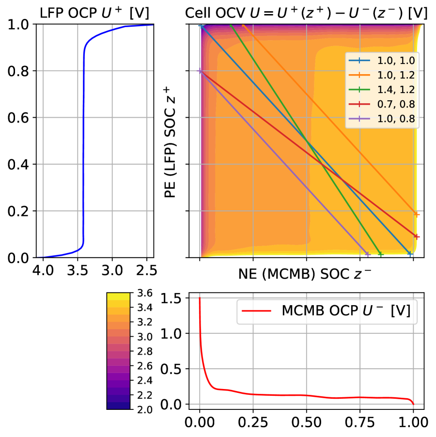
(a) $U_{\mathrm{OCV}}(z^{-},z^{+})$

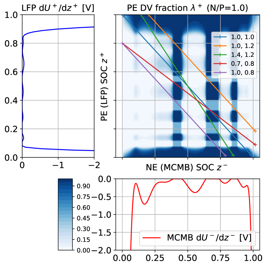
(b) PE DV fraction $\lambda^{+}(z^{-},z^{+};r_{\mathrm{N/P}})$

(c) $U_{\mathrm{OCV}}(z;r_{\mathrm{N/P}},z^{+}_{0})$

(d) $\lambda^{+}(z;r_{\mathrm{N/P}}=1,z^{+}_{0}=1)$

Figure 1: The assembly of electrode OCPs (left) and their derivatives (right) into the full-cell OCV and the PE differential voltage (DV) fraction, respectively, as well as how this assembly is affected by the N/P ratio $r_{\mathrm{N/P}}$ and Li/P ratio $z^{+}_{0}$. Top left: OCV square plots (advocated by Olson et al. [9]) of the LFP-graphite cell chemistry overlaid with five lines of $z^{+}(z^{-})$ corresponding to cells with different $(r_{\mathrm{N/P}},z^{+}_{0})$ pairs as indicated by the legends. Note that the color bar is associated with the contours. Bottom left: Various $z$-based OCV curves with different $(r_{\mathrm{N/P}},z^{+}_{0})$ pairs. Right: Counterparts of the left for the PE DV fraction, except that only a single $(r_{\mathrm{N/P}},z^{+}_{0})$ pair is shown on bottom right for clarity, where the peaks and troughs correspond to where the blue line in the top right figure crosses the dark and light areas.

Note that eq. 9 essentially comes from the inverse function $z^{-}(U_{\mathrm{OCV}})$ defined by (8) evaluated at $U_{\mathrm{min}}$ and $U_{\mathrm{max}}$ and is hence also parametrized by $r_{\mathrm{N/P}}$ and $z^{+}_{0}$. Therefore, the $z^{-}(z)$ from (10) and hence $U_{\mathrm{OCV}}(z)$ are parametrized by $r_{\mathrm{N/P}}$, $z^{+}_{0}$, $U_{\mathrm{min}}$, and $U_{\mathrm{max}}$, where given $U_{\mathrm{min}}$ and $U_{\mathrm{max}}$ fixed, $U_{\mathrm{OCV}}(z)$ is thus again parametrized by the independent and dimensionless $r_{\mathrm{N/P}}$ and $z^{+}_{0}$ only. This is the main difference from the parametrization of (2) based on four electrode SOC limits and two cutoff-voltage constraints [3]. Figures 1(a) and 1(c) (inspired by Olson et al. [9]) illustrate how $U_{\mathrm{OCV}}(z)$ is assembled from $U_{\mathrm{OCP}}^{\pm}(z^{\pm})$ and depends on $r_{\mathrm{N/P}}$ and $z^{+}_{0}$.

In this work, we will use the LFP-graphite chemistry as a running example and perform simulations coded in Python to concretely illustrate our results, where the electrode OCP relations are from the LFP and MCMB (mesocarbon microbeads, a form of synthetic graphite) OCP fits provided in Plett [4, sec. 3.11.1]. However, our results apply to all other chemistries and plots based on the NMC-graphite chemistry can also be found in the Supporting Information. For the LFP OCP, we choose the cutoff potential $2.5\mathrm{V}$ and $4.0\mathrm{V}$ to define $z^{+}=1$ and $z^{+}=0$, respectively, while the potential window defining $z^{-}=1$ and $z^{-}=0$ for MCMB is selected as $[0.0\mathrm{V},1.5\mathrm{V}]$. For the full cell, we use $U_{\mathrm{min}}=2.0\mathrm{V}$ to define the fully discharged state $z=0$ and $U_{\mathrm{max}}=3.6\mathrm{V}$ for the fully charged state $z=1$, which are common choices of cutoff voltage for LFP-graphite.

In fig. 1(a), line segments corresponding to cells with five $(r_{\mathrm{N/P}},z^{+}_{0})$ pairs are superposed on the 2D landscape of $U_{\mathrm{OCV}}(z^{-},z^{+})$, where the N/P ratio $r_{\mathrm{N/P}}$ is the negative slope and the Li/P ratio $z^{+}_{0}$ is the $z^{+}$-axis intercept. The $U_{\mathrm{min}}$-contour marks where these segments can start on the top left, while the $U_{\mathrm{max}}$-contour marks their possible ends on the bottom right. Then the slope $-r_{\mathrm{N/P}}$ and intercept $z^{+}_{0}$ determine whether the segment starts close to the top or left side of the square, and whether it ends near the bottom or right side. Therefore, this indicates the electrode SOC limits at the fully discharged and charged state, which implies which electrode is more limiting during discharging and charging, as will be further discussed in section 2.3. When we plot the OCV profile intersected by each segment and scale the segment to a unit interval, we obtain the $z$-based OCV $U_{\mathrm{OCV}}(z)$ in fig. 1(c). The flatness of the LFP and MCMB OCP makes the variation in $U_{\mathrm{OCV}}(z)$ rather mild visually with different $(r_{\mathrm{N/P}},z^{+}_{0})$ pairs, which will be precisely quantified in sections 2.4 and 3.1.

One advantage of the $z$-based OCV $U_{\mathrm{OCV}}(z)$ is that it can be determined directly by full-cell measurements without knowing anything about electrode OCP and SOC, just as how $U_{\mathrm{OCP}}^{\pm}(z^{\pm})$ can be determined agnostic of stoichiometry $x^{\pm}$. Moreover, this function can be roughly assumed unchanged upon aging [6] because by definition, $U_{\mathrm{OCV}}(z)$ always monotonically increases from $(0,U_{\mathrm{min}})$ to $(1,U_{\mathrm{max}})$, as fig. 1(c) illustrates. Hence, such electrode-agnostic monolithic cell OCV has been used in most ECMs in literature and in prevailing battery management systems [4, 5]. However, previous literature and the above have shown that $U_{\mathrm{OCV}}(z)$ does change appreciably upon aging, as further corroborated by fig. 2 based on simulations. Such variation encodes changes in $r_{\mathrm{N/P}}$ and $z^{+}_{0}$, and hence changes in degradation modes.

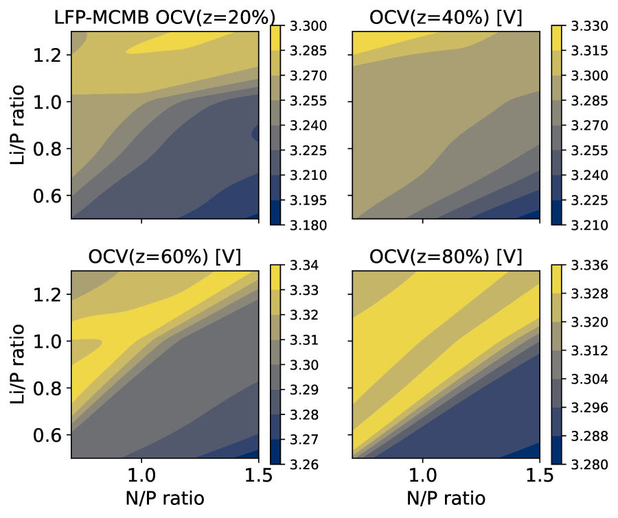
(a) $U_{\mathrm{OCV}}(z;r_{\mathrm{N/P}},z^{+}_{0})$

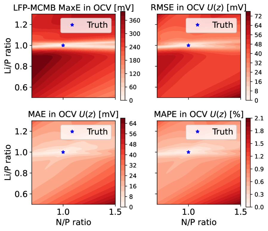
(b) $\|U_{\mathrm{OCV}}(z;r_{\mathrm{N/P}},z^{+}_{0})-U_{\mathrm{OCV}}(z;r_{\mathrm{N/P}}=1,z^{+}_{0}=1)\|$

Figure 2: Left: Cell OCV at SOC $z=20\%$, 40%, 60%, and 80% with different $(r_{\mathrm{N/P}},z^{+}_{0})$ pairs. Note the varied OCV sensitivity at different $z$’s. Right: Maximum errors (MaxE), Root-mean-square errors (RMSE), mean absolute errors (MAE), and mean absolute percentage errors (MAPE) between cell OCV with an arbitrary $(r_{\mathrm{N/P}},z^{+}_{0})$ pair and OCV with $r_{\mathrm{N/P}}=1$ and $z^{+}_{0}=1$ (marked as truth). Note in certain regions, RMSE and especially MaxE are relatively high but MAE is low, implying that the errors in the OCV curve are distributed very unevenly along $z$.

The upper and lower cutoff voltage also define the cell total capacity $\hat{Q}_{\mathrm{max}}$, which is the charge throughput associated with the SOC interval $0\leq z\leq 1$. The electrode SOC limits in (10) also relate the electrode capacity to their full-cell counterpart by charge conservation:

$$\hat{Q}_{\mathrm{max}}=(z_{\mathrm{max}}^{-}-z_{\mathrm{min}}^{-})\hat{Q}_{\mathrm{max}}^{-}=(z_{\mathrm{max}}^{+}-z_{\mathrm{min}}^{+})\hat{Q}_{\mathrm{max}}^{+}.$$ (12)

We have already mentioned that the four electrode SOC limits are parametrized by $r_{\mathrm{N/P}}$ and $z^{+}_{0}$ only, so $\hat{Q}_{\mathrm{max}}$ also depends on these two dimensionless quantities, but is additionally parametrized by the dimensional $\hat{Q}_{\mathrm{max}}^{+}$. Of course $\hat{Q}_{\mathrm{max}}^{+}$ is not the only choice, but in our opinion, it is the most natural and intuitive one since it is the denominator of both $r_{\mathrm{N/P}}$ and $z^{+}_{0}$. Equivalently, $\hat{Q}_{\mathrm{max}}$ can also be parametrized by the three-dimensional SOH parameter $\hat{Q}_{\mathrm{max}}^{\mathrm{Li}}$, $\hat{Q}_{\mathrm{max}}^{-}$, and $\hat{Q}_{\mathrm{max}}^{+}$. We will discuss the trade-off between these two options.

Since what Coulomb counting records is the charge or discharge throughput, sometimes we also want to express cell OCV in terms of, say charge throughput $\hat{Q}$, instead of the dimensionless SOC $z$. Assume $\hat{Q}$ counts from the fully discharged state at $U_{\mathrm{min}}$, we readily have $z=\hat{Q}/\hat{Q}_{\mathrm{max}}$ and it ultimately yields

$$U_{\mathrm{OCV}}(\hat{Q})=U^{+}_{\mathrm{OCP}}(z^{+}_{\mathrm{max}}-\hat{Q}/\hat{Q}_{\mathrm{max}}^{+})-U^{-}_{\mathrm{OCP}}(z^{-}_{\mathrm{min}}+\hat{Q}/\hat{Q}_{\mathrm{max}}^{-}),$$ (13)

which is essentially the same as (3) used by [11], except that $U_{\mathrm{OCV}}(\hat{Q})$ under our formulation here are parametrized by three independent SOH parameters $r_{\mathrm{N/P}}$, $z^{+}_{0}$, and $\hat{Q}_{\mathrm{max}}^{+}$ that do not depend on the choice of $U_{\mathrm{max}}$ or $U_{\mathrm{min}}$.

In the above analysis, we have assumed no LLI or LAM during charging or discharging. In practice, due to very slow degradation compared to charging and discharging, this is a good approximation within a few cycles and we only need to gradually adjust the SOH parameters upon cell aging. Even if we want to account for the minor degradation within a cycle, such as what manifests in Coulombic efficiency and capacity retention, the sensitivity gradients derived in the following lend us readily to a rigorous first-order analysis framework to be demonstrated in section 3.2.

2.3 Parametric Sensitivity: Electrode DV Fraction and Role of Fixed Cutoff Voltage

We first establish sensitivity results for a general parameter $\alpha$ of an electrode-specific cell OCV model $U_{\mathrm{OCV}}(z)$, which will then be applied to various specific SOH parameters. For the most general case, any input functional relation to eq. 11 that must be specified might depend on $\alpha$:

$$U_{\mathrm{OCP}}^{+}(z^{+},\alpha),\quad U_{\mathrm{OCP}}^{-}(z^{-},\alpha),\quad z^{+}(z^{-},\alpha),$$ (14)

which together constitute the final $U_{\mathrm{OCV}}(z,\alpha)$.

By the chain rule, we have (derivation details in Supporting Information)

$$\mathrm{\partial}_{\alpha}U_{\mathrm{OCV}}(z)= ~{}\mathrm{\partial}_{\alpha}U^{+}_{\mathrm{OCP}}(z^{+})+\mathrm{d}_{z^{+}}U^{+}_{\mathrm{OCP}}\cdot\mathrm{\partial}_{\alpha}z^{+}(z)$$ (15)

$$-\mathrm{\partial}_{\alpha}U^{-}_{\mathrm{OCP}}(z^{-})-\mathrm{d}_{z^{-}}U^{-}_{\mathrm{OCP}}\cdot\mathrm{\partial}_{\alpha}z^{-}(z),$$

$$\mathrm{\partial}_{\alpha}z^{+}(z)=\mathrm{\partial}_{\alpha}z^{+}(z^{-})-r_{\mathrm{N/P}}\mathrm{\partial}_{\alpha}z^{-}(z),$$ (16)

$$\mathrm{\partial}_{\alpha}z^{-}(z)=(1-z)\mathrm{\partial}_{\alpha}z^{-}_{\mathrm{min}}+z\mathrm{\partial}_{\alpha}z^{-}_{\mathrm{max}}.$$ (17)

$$\mathrm{\partial}_{\alpha}z^{-}(U_{\mathrm{OCV}})=\frac{\mathrm{\partial}_{\alpha}U_{\mathrm{OCP}}^{+}(z^{+})+\mathrm{d}_{z^{+}}U_{\mathrm{OCP}}^{+}\cdot\mathrm{\partial}_{\alpha}z^{+}(z^{-})-\mathrm{\partial}_{\alpha}U_{\mathrm{OCP}}^{-}(z^{-})}{r_{\mathrm{N/P}}\mathrm{d}_{z^{+}}U_{\mathrm{OCP}}^{+}+\mathrm{d}_{z^{-}}U_{\mathrm{OCP}}^{-}}.$$ (18)

$$\mathrm{\partial}_{\alpha}z^{-}_{\mathrm{min}}=\mathrm{\partial}_{\alpha}z^{-}(U_{\mathrm{min}}),\qquad\mathrm{\partial}_{\alpha}z^{-}_{\mathrm{max}}=\mathrm{\partial}_{\alpha}z^{-}(U_{\mathrm{max}}).$$ (19)

One subtlety here is that $z^{-}_{\mathrm{min}}$ is defined implicitly by the lower cutoff voltage as $U_{\mathrm{OCV}}(z^{-}_{\mathrm{min}})=U_{\mathrm{min}}$. Therefore, calculating $\mathrm{\partial}_{\alpha}z^{-}_{\mathrm{min}}$ reduces to differentiating the implicit function $z^{-}(U_{\mathrm{OCV}},\alpha)$ defined by $U_{\mathrm{OCV}}(z^{-},\alpha)$.

Since generically, we have $\mathrm{\partial}_{\alpha}z^{\pm}(z)\neq 0$, the change of $\alpha$ may cause the same $z$ to correspond to a different $z^{\pm}$. In particular, the electrode SOC limits $z^{-}_{\mathrm{min}}$, $z^{-}_{\mathrm{max}}$, $z^{+}_{\mathrm{min}}$, and $z^{+}_{\mathrm{max}}$ at the upper and lower cutoff voltage can change with $\alpha$, causing the “charge/discharge end-point slippage” [17, 16]. In contrast, the PE-NE relative slippage indicated by $\mathrm{\partial}_{\alpha}z^{+}(z^{-})\neq 0$ causing one $z^{-}$ to correspond to a different $z^{+}$ will also occur unless both $r_{\mathrm{N/P}}$ and $z^{+}_{0}$ are fixed, i.e. the ratio $\hat{Q}_{\mathrm{max}}^{-}:\hat{Q}_{\mathrm{max}}^{+}:\hat{Q}_{\mathrm{max}}^{\mathrm{Li}}$ stays the same. A lot of researchers have studied such electrode slippage due to SEI growth during charging, but what we have derived above reveal a bigger picture of other potential underlying mechanisms.

The $z^{-}(z)$ and $z^{+}(z)$ slippage also causes the electrode potential $U^{\pm}_{\mathrm{OCV}}(z^{\pm}(z))$ and consequently the cell OCV $U_{\mathrm{OCV}}(z)$ to change for a particular $z$. Therefore, a certain cell SOC $z$ does not anchor to any electrode SOC $z^{\pm}$ or any OCV value (except for $z=0$ and $z=1$ in the latter case). The cell SOC $z$ simply indicates the relative remaining discharge throughput against total capacity $\hat{Q}_{\mathrm{max}}$ until fully discharged. This is probably the only persistent physical meaning of a so-defined cell SOC $z$.

In addition to the cell OCV $U_{\mathrm{OCV}}(z)$ that is independent of the total capacity, we can also characterize the parametric sensitivity of total capacity $\hat{Q}_{\mathrm{max}}=(z_{\mathrm{max}}^{-}-z_{\mathrm{min}}^{-})\hat{Q}_{\mathrm{max}}^{-}$ by

$$\mathrm{\partial}_{\alpha}\hat{Q}_{\mathrm{max}}=(\mathrm{\partial}_{\alpha}z_{\mathrm{max}}^{-}-\mathrm{\partial}_{\alpha}z_{\mathrm{min}}^{-})\hat{Q}_{\mathrm{max}}^{-}+(z_{\mathrm{max}}^{-}-z_{\mathrm{min}}^{-})\mathrm{\partial}_{\alpha}\hat{Q}_{\mathrm{max}}^{-}.$$ (20)

Any particular parameter will usually not appear in all three funcitonal relations in (14), which will thus simplify eqs. 15, 16, 17, 18 and 19. There are two main types of such cases. The first type is a parameter that only affects the two electrode OCP relations but not $z^{+}(z^{-})$, such as temperature [4] or parameters governing the component changes in composite electrode active materials [18] if they do not also affect the electrode capacity. In this case, eqs. 16 and 18 reduce to

$$\mathrm{\partial}_{\alpha}z^{+}(z)=-r_{\mathrm{N/P}}\mathrm{\partial}_{\alpha}z^{-}(z),$$ (21)

$$\mathrm{\partial}_{\alpha}z^{-}(U_{\mathrm{OCV}})=\frac{\mathrm{\partial}_{\alpha}U_{\mathrm{OCP}}^{+}(z^{+})-\mathrm{\partial}_{\alpha}U_{\mathrm{OCP}}^{-}(z^{-})}{r_{\mathrm{N/P}}\mathrm{d}_{z^{+}}U_{\mathrm{OCP}}^{+}+\mathrm{d}_{z^{-}}U_{\mathrm{OCP}}^{-}}.$$ (22)

We will not look into this type of parameters in this work.

The other type includes $r_{\mathrm{N/P}}$ and $z^{+}_{0}$ or their reparametrization, which are related to LLI and LAM and affect only $z^{+}(z^{-})$ but not the electrode OCP. In this case, eqs. 15 and 18 reduce to:

$$\mathrm{\partial}_{\alpha}U_{\mathrm{OCV}}(z)=\mathrm{d}_{z^{+}}U^{+}_{\mathrm{OCP}}\cdot\mathrm{\partial}_{\alpha}z^{+}(z)-\mathrm{d}_{z^{-}}U^{-}_{\mathrm{OCP}}\cdot\mathrm{\partial}_{\alpha}z^{-}(z),$$ (23)

$$\mathrm{\partial}_{\alpha}z^{-}(U_{\mathrm{OCV}})=\frac{\mathrm{d}_{z^{+}}U_{\mathrm{OCP}}^{+}}{r_{\mathrm{N/P}}\mathrm{d}_{z^{+}}U_{\mathrm{OCP}}^{+}+\mathrm{d}_{z^{-}}U_{\mathrm{OCP}}^{-}}\mathrm{\partial}_{\alpha}z^{+}(z^{-}).$$ (24)

The physical meaning of the apparently complicated fraction coefficient in (24) can be revealed by defining the dimensional counterparts of the electrode and cell SOC as

$$\hat{Q}^{\pm}=z^{\pm}\hat{Q}^{\pm}_{\mathrm{max}},\qquad\hat{Q}=z\hat{Q}_{\mathrm{max}},$$ (25)

and with charge conservation $\mathrm{d}\hat{Q}=\mathrm{d}\hat{Q}^{-}=-\mathrm{d}\hat{Q}^{+}$, rewriting the fraction as

$$\frac{1}{r_{\mathrm{N/P}}}\frac{r_{\mathrm{N/P}}\mathrm{d}_{z^{+}}U_{\mathrm{OCP}}^{+}}{r_{\mathrm{N/P}}\mathrm{d}_{z^{+}}U_{\mathrm{OCP}}^{+}+\mathrm{d}_{z^{-}}U_{\mathrm{OCP}}^{-}}=\frac{1}{r_{\mathrm{N/P}}}\frac{\mathrm{d}_{\hat{Q}^{+}}U_{\mathrm{OCP}}^{+}}{\mathrm{d}_{\hat{Q}^{+}}U_{\mathrm{OCP}}^{+}+\mathrm{d}_{\hat{Q}^{-}}U_{\mathrm{OCP}}^{-}}=\frac{1}{r_{\mathrm{N/P}}}\frac{\mathrm{d}_{\hat{Q}}U_{\mathrm{OCP}}^{+}}{\mathrm{d}_{\hat{Q}}U_{\mathrm{OCV}}}.$$

Since $\mathrm{d}_{\hat{Q}^{+}}U_{\mathrm{OCP}}^{+}$ and $\mathrm{d}_{\hat{Q}^{-}}U_{\mathrm{OCP}}^{-}$ are both negative, the second fraction factor above can be interpreted as the fraction of the PE contribution to the full-cell differential voltage.

Due to the important role played by this fraction in subsequent sensitivity gradients and its clear physical meaning, we call it the PE DV (differential voltage) fraction and denote it by

$$\lambda^{+}=\frac{r_{\mathrm{N/P}}\mathrm{d}_{z^{+}}U_{\mathrm{OCP}}^{+}}{r_{\mathrm{N/P}}\mathrm{d}_{z^{+}}U_{\mathrm{OCP}}^{+}+\mathrm{d}_{z^{-}}U_{\mathrm{OCP}}^{-}}=\frac{\mathrm{d}_{\hat{Q}^{+}}U_{\mathrm{OCP}}^{+}}{\mathrm{d}_{\hat{Q}^{+}}U_{\mathrm{OCP}}^{+}+\mathrm{d}_{\hat{Q}^{-}}U_{\mathrm{OCP}}^{-}}\in[0,1]$$ (26)

and the NE DV fraction is simply $\lambda^{-}=1-\lambda^{+}$. Figures 1(b) and 1(d) show $\lambda^{+}(z^{-},z^{+})$ and how $\lambda^{+}(z)$ is obtained analogously to how $U_{\mathrm{OCV}}(z)$ is obtained from $U_{\mathrm{OCV}}(z^{-},z^{+})$ in figs. 1(a) and 1(c). Note that compared to $U_{\mathrm{OCV}}(z^{-},z^{+})$, which is independent of $r_{\mathrm{N/P}}$ or $z^{+}_{0}$, $\lambda^{+}(z^{-},z^{+})$ as defined by 26 does depend on $r_{\mathrm{N/P}}$, although empirically this dependence is weak and does not alter the overall pattern of $\lambda^{+}(z^{-},z^{+})$. Therefore, we still overlay the $\lambda^{+}$ landscape at $r_{\mathrm{N/P}}=1$ in fig. 1(b) with segments of different $(r_{\mathrm{N/P}},z^{+}_{0})$ pairs for illustration.

Figure 3: Electrode SOC limits (left) and cathode DV fractions (right) at different N/P ratio $r_{\mathrm{N/P}}$ and Li/P ratio $z^{+}_{0}$. The top row regards the fully charged state $U_{\mathrm{OCV}}=U_{\mathrm{max}}$, where the variation mostly depends on $z^{+}_{0}/r_{\mathrm{N/P}}$, which is essentially the Li/N ratio, and has a sharp change at $z^{+}_{0}/r_{\mathrm{N/P}}=1$. In contrast, the bottom is at the fully discharged state $U_{\mathrm{OCV}}=U_{\mathrm{min}}$, whose variation mostly depends on the Li/P ratio and has a sharp change at $z^{+}_{0}=1$.

Since in eq. 17, we only need (24) at the lower and upper cutoff voltage, we specifically define

$$\lambda^{+}_{\mathrm{l}}=\frac{r_{\mathrm{N/P}}\left.\mathrm{d}_{z^{+}}U_{\mathrm{OCP}}^{+}\right|_{z^{+}_{\mathrm{max}}}}{r_{\mathrm{N/P}}\left.\mathrm{d}_{z^{+}}U_{\mathrm{OCP}}^{+}\right|_{z^{+}_{\mathrm{max}}}+\left.\mathrm{d}_{z^{-}}U_{\mathrm{OCP}}^{-}\right|_{z^{-}_{\mathrm{min}}}},\quad\lambda^{+}_{\mathrm{u}}=\frac{r_{\mathrm{N/P}}\left.\mathrm{d}_{z^{+}}U_{\mathrm{OCP}}^{+}\right|_{z^{+}_{\mathrm{min}}}}{r_{\mathrm{N/P}}\left.\mathrm{d}_{z^{+}}U_{\mathrm{OCP}}^{+}\right|_{z^{+}_{\mathrm{min}}}+\left.\mathrm{d}_{z^{-}}U_{\mathrm{OCP}}^{-}\right|_{z^{-}_{\mathrm{max}}}}$$ (27)

associated with $U_{\mathrm{min}}$ and $U_{\mathrm{max}}$, respectively. The above also implies that the sole reason why the electrode DV fractions play a role in our sensitivity analysis is the dependence of cell SOC $z$ and total capacity $\hat{Q}_{\mathrm{max}}$ on the arbitrarily specified lower and upper cutoff voltage.

The PE DV fraction $\lambda^{+}_{\mathrm{u}}$ and $\lambda^{+}_{\mathrm{l}}$ also quantify to what extent each electrode limits the charging or discharging towards the respective cutoff voltage, which has been studied in the context of discerning Coulombic efficiency and capacity retention [19, 16]. When $\lambda^{+}_{\mathrm{l}}\approx 1$, it implies that the cell reaches $U_{\mathrm{min}}$ in discharging mainly because the PE gets filled up with $\mathrm{Li}^{+}$ due to $\hat{Q}_{\mathrm{max}}^{\mathrm{Li}}>\hat{Q}_{\mathrm{max}}^{+}$, or equivalently $z^{+}_{0}>1$, so its potential sharply drops, which is called PE-limited discharging. In contrast, when $\lambda^{+}_{\mathrm{l}}\approx 0$, the cell reaches $U_{\mathrm{min}}$ mostly due to the $\mathrm{Li}^{+}$ depletion in the NE and thus the steep rise of its potential, hence called NE-limited discharging. We can likewise define PE- and NE-limited charging. Figure 3 illustrates how the electrode SOC limits and PE DV fractions vary with the N/P ratio $r_{\mathrm{N/P}}$ and Li/P ratio $z^{+}_{0}$, which can be divided into four quadrants depending on whether $z^{+}_{0}>1$ and $z^{+}_{0}>r_{\mathrm{N/P}}$, or more intuitively, whether $\hat{Q}_{\mathrm{max}}^{\mathrm{Li}}>\hat{Q}_{\mathrm{max}}^{+}$ and $\hat{Q}_{\mathrm{max}}^{\mathrm{Li}}>\hat{Q}_{\mathrm{max}}^{-}$. We will go into more depth concerning these four regimes in section 2.5.

With the introduction of the PE DV fraction $\lambda^{+}$, eq. 19 simplifies to

$$\mathrm{\partial}_{\alpha}z^{-}_{\mathrm{min}}=\frac{\lambda^{+}_{\mathrm{l}}}{r_{\mathrm{N/P}}}\mathrm{\partial}_{\alpha}z^{+}(z^{-}_{\mathrm{min}}),\quad\mathrm{\partial}_{\alpha}z^{-}_{\mathrm{max}}=\frac{\lambda^{+}_{\mathrm{u}}}{r_{\mathrm{N/P}}}\mathrm{\partial}_{\alpha}z^{+}(z^{-}_{\mathrm{max}}),$$ (28)

which paves the way for deriving the sensitivity gradients with respect to $r_{\mathrm{N/P}}$ and $z^{+}_{0}$.

2.4 SOH-Sensitivity Gradients of Electrode SOC Limits and Cell OCV

Before proceeding, we must point out a subtlety omitted in previous parts. A partial derivative with respect to a particular parameter $\alpha$ itself is ambiguous, because it also depends on the complete parametrization, i.e. choices of parameters other than $\alpha$. All the previous results still hold, but we must specify the full set of parameters before carrying out concrete calculations.

We know that $U_{\mathrm{OCV}}(z)$ can be parametrized by $r_{\mathrm{N/P}}$ and $z^{+}_{0}$, so $(r_{\mathrm{N/P}},z^{+}_{0})$ serves as the complete parameter set for the following partial differentiation. From eq. 6, we can easily obtain

$$\mathrm{\partial}_{r_{\mathrm{N/P}}}z^{+}(z^{-})=-z^{-},\qquad\mathrm{\partial}_{z^{+}_{0}}z^{+}(z^{-})=1.$$ (29)

We first derive the counterparts of eqs. 15, 16, 17, 18 and 19 for $r_{\mathrm{N/P}}$:

$$\frac{\mathrm{\partial}z^{-}(U_{\mathrm{OCV}})}{\mathrm{\partial}r_{\mathrm{N/P}}}=\left.\frac{-z^{-}\lambda^{+}}{r_{\mathrm{N/P}}}\right|_{U_{\mathrm{OCV}}},$$ (30)

$$\frac{\mathrm{\partial}z^{-}_{\mathrm{min}}}{\mathrm{\partial}r_{\mathrm{N/P}}}=\frac{-z^{-}_{\mathrm{min}}\lambda^{+}_{\mathrm{l}}}{r_{\mathrm{N/P}}},\qquad\frac{\mathrm{\partial}z^{-}_{\mathrm{max}}}{\mathrm{\partial}r_{\mathrm{N/P}}}=\frac{-z^{-}_{\mathrm{max}}\lambda^{+}_{\mathrm{u}}}{r_{\mathrm{N/P}}},$$ (31)

$$\frac{\mathrm{\partial}z^{-}(z)}{\mathrm{\partial}r_{\mathrm{N/P}}}=-\frac{(1-z)z^{-}_{\mathrm{min}}\lambda^{+}_{\mathrm{l}}+zz^{-}_{\mathrm{max}}\lambda^{+}_{\mathrm{u}}}{r_{\mathrm{N/P}}},\qquad\frac{\mathrm{\partial}z^{+}(z)}{\mathrm{\partial}r_{\mathrm{N/P}}}=-(1-z)z^{-}_{\mathrm{min}}\lambda^{-}_{\mathrm{l}}-zz^{-}_{\mathrm{max}}\lambda^{-}_{\mathrm{u}},$$ (32)

$$\frac{\mathrm{\partial}U_{\mathrm{OCV}}(z)}{\mathrm{\partial}r_{\mathrm{N/P}}}=\frac{\mathrm{d}U^{+}_{\mathrm{OCP}}}{\mathrm{d}z^{+}}\frac{\mathrm{\partial}z^{+}(z)}{\mathrm{\partial}r_{\mathrm{N/P}}}-\frac{\mathrm{d}U^{-}_{\mathrm{OCP}}}{\mathrm{d}z^{-}}\frac{\mathrm{\partial}z^{-}(z)}{\mathrm{\partial}r_{\mathrm{N/P}}}.$$ (33)

As we can see, both $\mathrm{\partial}_{r_{\mathrm{N/P}}}z^{\pm}(z)$ vary linearly with $z$, which is not surprising since $z^{\pm}(z)$ have to remain linear by definition of $z$.

(a) $U_{\mathrm{OCV}}(z^{-};r_{\mathrm{N/P}},z^{+}_{0}=1)$

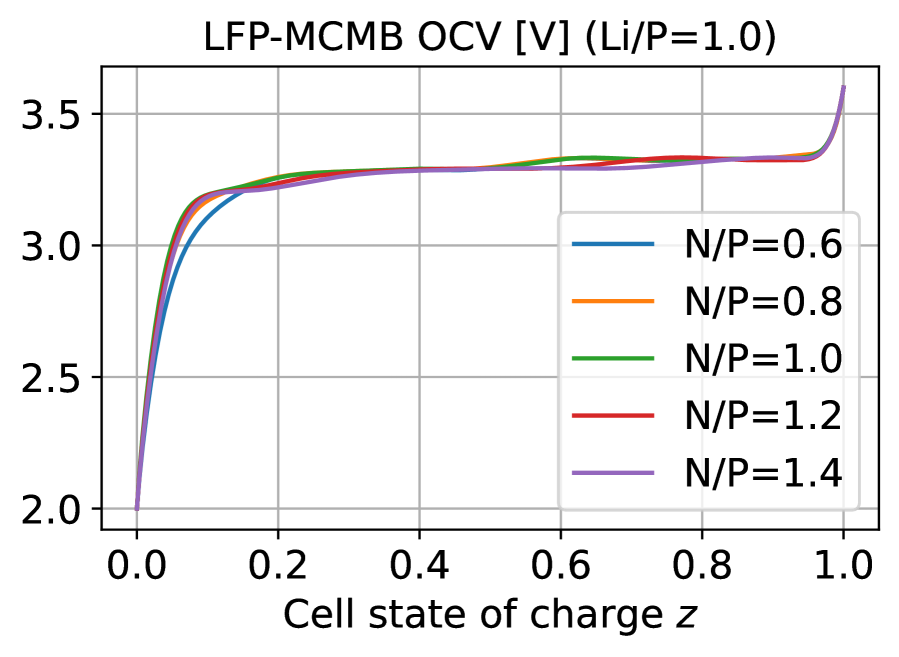
(b) $U_{\mathrm{OCV}}(z;r_{\mathrm{N/P}},z^{+}_{0}=1)$

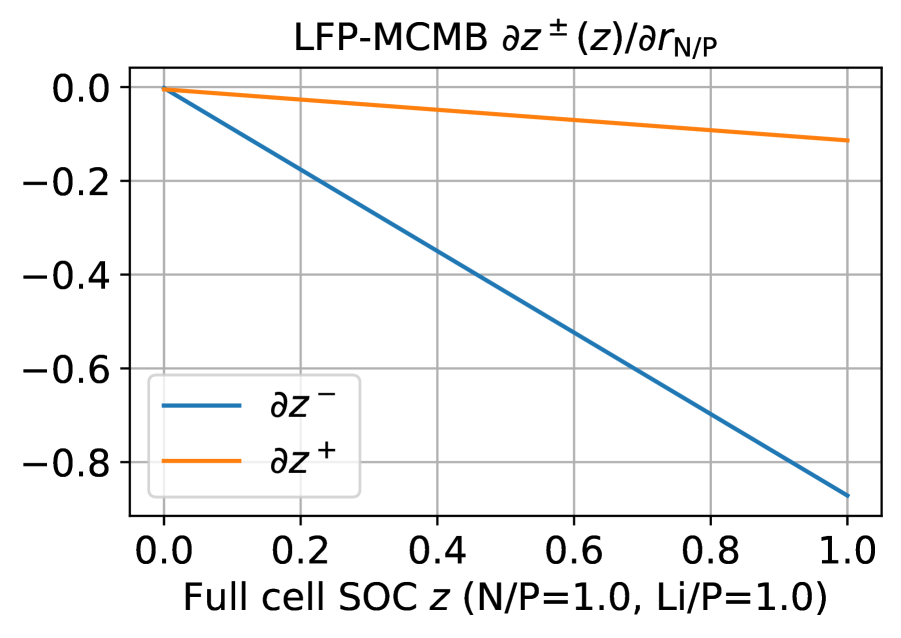
(c) $\mathrm{\partial}_{r_{\mathrm{N/P}}}z^{\pm}(z;r_{\mathrm{N/P}}=1,z^{+}_{0}=1)$

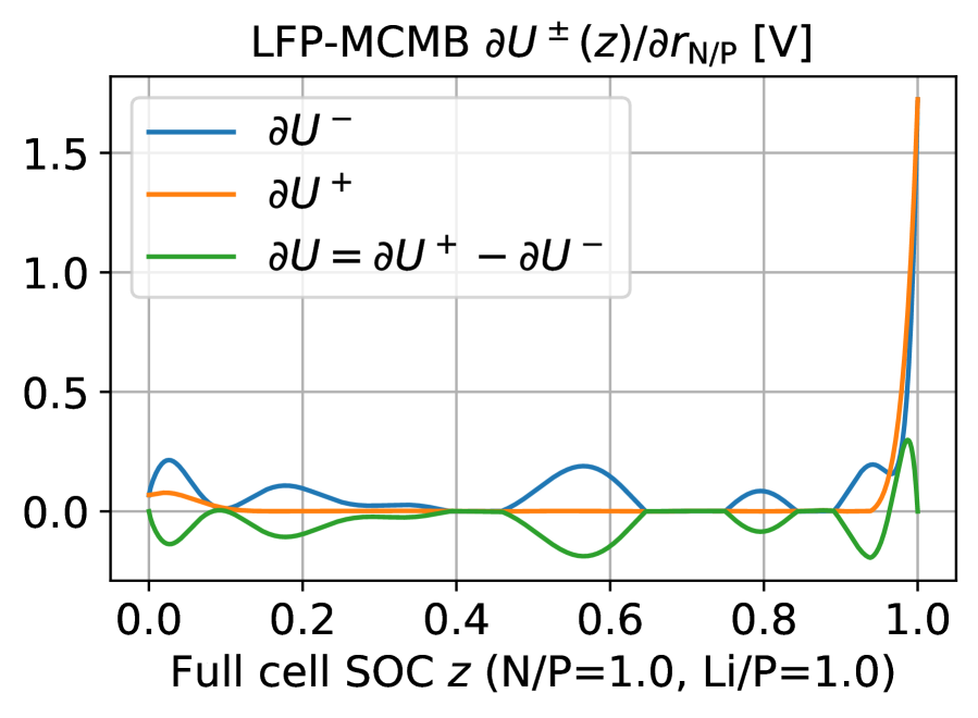
(d) $\mathrm{\partial}_{r_{\mathrm{N/P}}}U_{\mathrm{OCP}}^{\pm}(z)$ and $\mathrm{\partial}_{r_{\mathrm{N/P}}}U_{\mathrm{OCV}}(z)$

Figure 4: Top: Variation of $z^{-}$-based (top left) and $z$-based (top right) cell OCV when $r_{\mathrm{N/P}}$ changes and $z^{+}_{0}=1$. Bottom: Derivative-based local sensitivity of $z^{\pm}(z)$ (bottom left) and of $z$-based electrode OCPs and cell OCV (bottom right) with respect to $r_{\mathrm{N/P}}$. All the sensitivity derivatives are evaluated at $r_{\mathrm{N/P}}=1$ and $z^{+}_{0}=1$.

Figure 4 demonstrates empirically how the $z^{-}$-based OCV $U_{\mathrm{OCV}}(z^{-})$ and $z$-based OCV $U_{\mathrm{OCV}}(z)$ vary with the N/P ratio $r_{\mathrm{N/P}}$ on the top, and the $r_{\mathrm{N/P}}$-derivatives $\mathrm{\partial}_{r_{\mathrm{N/P}}}z^{\pm}(z)$, $\mathrm{\partial}_{r_{\mathrm{N/P}}}U_{\mathrm{OCP}}^{\pm}(z)$, and $\mathrm{\partial}_{r_{\mathrm{N/P}}}U_{\mathrm{OCV}}(z)$ evaluated at $r_{\mathrm{N/P}}=1$. Figure 4(a) shows that $z^{-}_{\mathrm{max}}$ quickly decreases with increasing $r_{\mathrm{N/P}}$, while $z^{-}_{\mathrm{min}}$ is insensitive to $r_{\mathrm{N/P}}$ in this case, which is consistent with $\mathrm{\partial}_{r_{\mathrm{N/P}}}z^{-}(z=1)<-0.8$ and $\mathrm{\partial}_{r_{\mathrm{N/P}}}z^{-}(z=0)\approx 0$ as indicated by fig. 4(c). On the other hand, due to the OCP curves in both electrodes being rather flat for a large mid-SOC range, $U_{\mathrm{OCV}}(z)$ is not very sensitive to $r_{\mathrm{N/P}}$ overall (fig. 4(b)) and the several narrow SOC windows with relatively high sensitivity are also aligned with what the $r_{\mathrm{N/P}}$-derivatives imply in fig. 4(d).

Next, we carry out the same sensitivity analysis with respect to $z^{+}_{0}$:

$$\frac{\mathrm{\partial}z^{-}(U_{\mathrm{OCV}})}{\mathrm{\partial}z^{+}_{0}}=\left.\frac{\lambda^{+}}{r_{\mathrm{N/P}}}\right|_{U_{\mathrm{OCV}}},$$ (34)

$$\frac{\mathrm{\partial}z^{-}_{\mathrm{min}}}{\mathrm{\partial}z^{+}_{0}}=\frac{\lambda^{+}_{\mathrm{l}}}{r_{\mathrm{N/P}}},\qquad\frac{\mathrm{\partial}z^{-}_{\mathrm{max}}}{\mathrm{\partial}z^{+}_{0}}=\frac{\lambda^{+}_{\mathrm{u}}}{r_{\mathrm{N/P}}},$$ (35)

$$\frac{\mathrm{\partial}z^{-}(z)}{\mathrm{\partial}z^{+}_{0}}=\frac{(1-z)\lambda^{+}_{\mathrm{l}}+z\lambda^{+}_{\mathrm{u}}}{r_{\mathrm{N/P}}},\qquad\frac{\mathrm{\partial}z^{+}(z)}{\mathrm{\partial}z^{+}_{0}}=(1-z)\lambda^{-}_{\mathrm{l}}+z\lambda^{-}_{\mathrm{u}},$$ (36)

$$\frac{\mathrm{\partial}U_{\mathrm{OCV}}(z)}{\mathrm{\partial}z^{+}_{0}}=\frac{\mathrm{d}U^{+}_{\mathrm{OCP}}}{\mathrm{d}z^{+}}\frac{\mathrm{\partial}z^{+}(z)}{\mathrm{\partial}z^{+}_{0}}-\frac{\mathrm{d}U^{-}_{\mathrm{OCP}}}{\mathrm{d}z^{-}}\frac{\mathrm{\partial}z^{-}(z)}{\mathrm{\partial}z^{+}_{0}}.$$ (37)

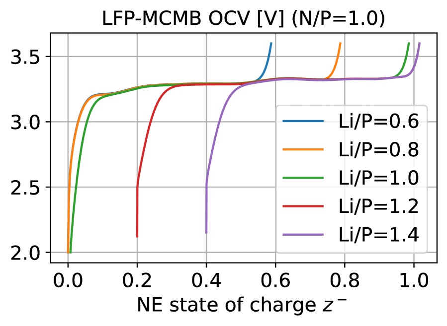
(a) $U_{\mathrm{OCV}}(z^{-};r_{\mathrm{N/P}}=1,z^{+}_{0})$

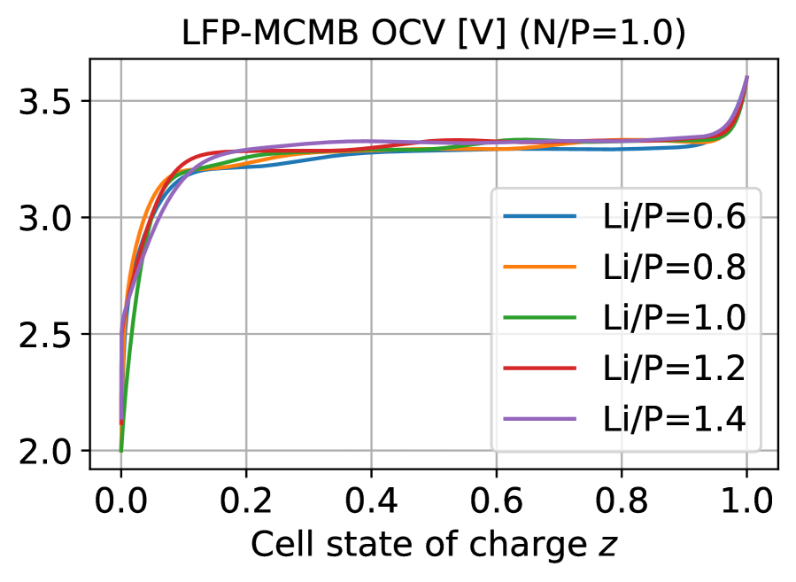
(b) $U_{\mathrm{OCV}}(z;r_{\mathrm{N/P}}=1,z^{+}_{0})$

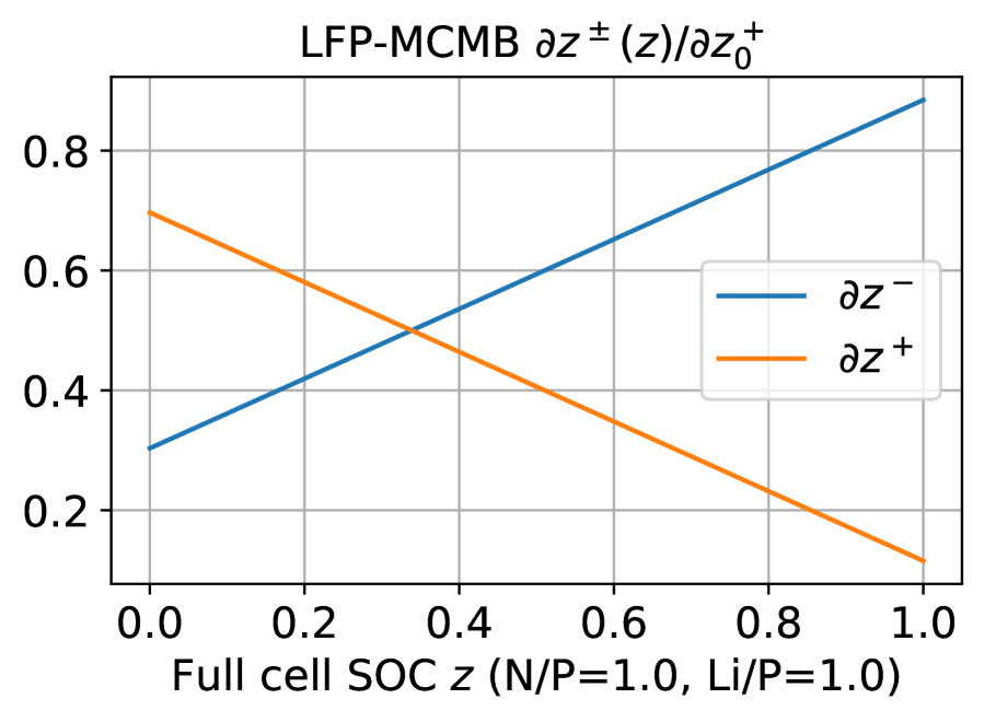
(c) $\mathrm{\partial}_{z^{+}_{0}}z^{\pm}(z;r_{\mathrm{N/P}}=1,z^{+}_{0}=1)$

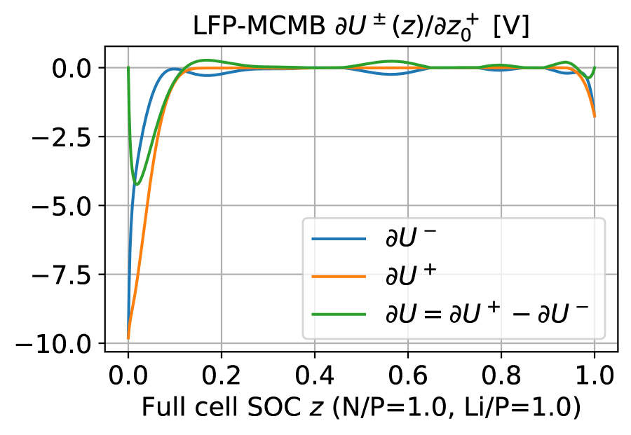
(d) $\mathrm{\partial}_{z^{+}_{0}}U_{\mathrm{OCP}}^{\pm}(z)$ and $\mathrm{\partial}_{z^{+}_{0}}U_{\mathrm{OCV}}(z)$

Figure 5: Top: Variation of $z^{-}$-based (top left) and $z$-based (top right) cell OCV when Li/P ratio $z^{+}_{0}$ changes and $r_{\mathrm{N/P}}=1$. Bottom: Derivative-based local sensitivity of $z^{\pm}(z)$ (bottom left) and of $z$-based electrode OCPs and cell OCV (bottom right) with respect to $z^{+}_{0}$. All the sensitivity derivatives are evaluated at $r_{\mathrm{N/P}}=1$ and $z^{+}_{0}=1$.

Again, fig. 5, which is the $z^{+}_{0}$-counterpart of fig. 4, shows the consistency between empirical and analytical sensitivity results. Note that the electrode SOC limits always increase with the lithium inventory as implied by figs. 5(a) and 5(c), which is also consistent with fig. 3.

2.5 SOH-Sensitivity Gradients of Total Capacity: Four Characteristic Regimes

Besides for the cell OCV $U_{\mathrm{OCV}}(z)$, we can also compute the sensitivity derivatives for the total capacity $\hat{Q}_{\mathrm{max}}=(z_{\mathrm{max}}^{-}-z_{\mathrm{min}}^{-})r_{\mathrm{N/P}}\hat{Q}_{\mathrm{max}}^{+}$ by eq. 20. Note, however, that besides the dimensionless $r_{\mathrm{N/P}}$ and $z^{+}_{0}$, $\hat{Q}_{\mathrm{max}}$ also depends on the dimensional $\hat{Q}_{\mathrm{max}}^{+}$. Therefore, for $\hat{Q}_{\mathrm{max}}(r_{\mathrm{N/P}},z^{+}_{0},\hat{Q}_{\mathrm{max}}^{+})$, we can obtain the following parameter-derivatives:

$$\frac{\mathrm{\partial}\hat{Q}_{\mathrm{max}}}{\mathrm{\partial}r_{\mathrm{N/P}}}=(z^{-}_{\mathrm{max}}\lambda^{-}_{\mathrm{u}}-z^{-}_{\mathrm{min}}\lambda^{-}_{\mathrm{l}})\hat{Q}_{\mathrm{max}}^{+},\quad\frac{\mathrm{\partial}\hat{Q}_{\mathrm{max}}}{\mathrm{\partial}z^{+}_{0}}=(\lambda^{+}_{\mathrm{u}}-\lambda^{+}_{\mathrm{l}})\hat{Q}_{\mathrm{max}}^{+},\quad\frac{\mathrm{\partial}\hat{Q}_{\mathrm{max}}}{\mathrm{\partial}\hat{Q}_{\mathrm{max}}^{+}}=(z_{\mathrm{max}}^{-}-z_{\mathrm{min}}^{-})r_{\mathrm{N/P}}$$ (38)

where we have used eqs. 31 and 35.

In contrast to $U_{\mathrm{OCV}}(z)$, the total capacity $\hat{Q}_{\mathrm{max}}$ can be alternatively parametrized by $\hat{Q}_{\mathrm{max}}^{\mathrm{Li}}$, $\hat{Q}_{\mathrm{max}}^{-}$, and $\hat{Q}_{\mathrm{max}}^{+}$, all of which are of the same dimension of charges. To derive the parametric derivatives for this case, one subtlety is that we need to translate $z^{+}(z^{-};r_{\mathrm{N/P}},z^{+}_{0})$ to

$$z^{+}(z^{-};\hat{Q}_{\mathrm{max}}^{\mathrm{Li}},\hat{Q}_{\mathrm{max}}^{-},\hat{Q}_{\mathrm{max}}^{+})=\frac{\hat{Q}_{\mathrm{max}}^{\mathrm{Li}}}{\hat{Q}_{\mathrm{max}}^{+}}-\frac{\hat{Q}_{\mathrm{max}}^{-}}{\hat{Q}_{\mathrm{max}}^{+}}z^{-},$$ (39)

which yields

$$\frac{\mathrm{\partial}z^{+}(z^{-})}{\mathrm{\partial}\hat{Q}_{\mathrm{max}}^{\mathrm{Li}}}=\frac{1}{\hat{Q}_{\mathrm{max}}^{+}},\qquad\frac{\mathrm{\partial}z^{+}(z^{-})}{\mathrm{\partial}\hat{Q}_{\mathrm{max}}^{-}}=\frac{-z^{-}}{\hat{Q}_{\mathrm{max}}^{+}},\qquad\frac{\mathrm{\partial}z^{+}(z^{-})}{\mathrm{\partial}\hat{Q}_{\mathrm{max}}^{+}}=\frac{-z^{+}}{\hat{Q}_{\mathrm{max}}^{+}}.$$ (40)

Note that in deriving (38), we have implicitly used

$$\frac{\mathrm{\partial}z^{+}(z^{-};r_{\mathrm{N/P}},z^{+}_{0},\hat{Q}_{\mathrm{max}}^{+})}{\mathrm{\partial}\hat{Q}_{\mathrm{max}}^{+}}=0\neq\frac{\mathrm{\partial}z^{+}(z^{-};\hat{Q}_{\mathrm{max}}^{\mathrm{Li}},\hat{Q}_{\mathrm{max}}^{-},\hat{Q}_{\mathrm{max}}^{+})}{\mathrm{\partial}\hat{Q}_{\mathrm{max}}^{+}},$$

which examplifies the partial differentiation ambiguity without specifying the complete parametrization as mentioned. Now using eq. 28, we have

$$\frac{\mathrm{\partial}z^{-}_{\mathrm{min}}}{\mathrm{\partial}\hat{Q}_{\mathrm{max}}^{\mathrm{Li}}}=\frac{\lambda^{+}_{\mathrm{l}}}{\hat{Q}_{\mathrm{max}}^{-}},\qquad\frac{\mathrm{\partial}z^{-}_{\mathrm{max}}}{\mathrm{\partial}\hat{Q}_{\mathrm{max}}^{\mathrm{Li}}}=\frac{\lambda^{+}_{\mathrm{u}}}{\hat{Q}_{\mathrm{max}}^{-}},$$ (41)

$$\frac{\mathrm{\partial}z^{-}_{\mathrm{min}}}{\mathrm{\partial}\hat{Q}_{\mathrm{max}}^{-}}=\frac{-z^{-}_{\mathrm{min}}\lambda^{+}_{\mathrm{l}}}{\hat{Q}_{\mathrm{max}}^{-}},\qquad\frac{\mathrm{\partial}z^{-}_{\mathrm{max}}}{\mathrm{\partial}\hat{Q}_{\mathrm{max}}^{-}}=\frac{-z^{-}_{\mathrm{max}}\lambda^{+}_{\mathrm{u}}}{\hat{Q}_{\mathrm{max}}^{-}},$$ (42)

$$\frac{\mathrm{\partial}z^{-}_{\mathrm{min}}}{\mathrm{\partial}\hat{Q}_{\mathrm{max}}^{+}}=\frac{-z^{+}_{\mathrm{max}}\lambda^{+}_{\mathrm{l}}}{\hat{Q}_{\mathrm{max}}^{-}},\qquad\frac{\mathrm{\partial}z^{-}_{\mathrm{max}}}{\mathrm{\partial}\hat{Q}_{\mathrm{max}}^{+}}=\frac{-z^{+}_{\mathrm{min}}\lambda^{+}_{\mathrm{u}}}{\hat{Q}_{\mathrm{max}}^{-}},$$ (43)

which by eq. 20, finally give the sensitivity derivatives:

$$\frac{\mathrm{\partial}\hat{Q}_{\mathrm{max}}}{\mathrm{\partial}\hat{Q}_{\mathrm{max}}^{\mathrm{Li}}}=\lambda^{+}_{\mathrm{u}}-\lambda^{+}_{\mathrm{l}},\qquad\frac{\mathrm{\partial}\hat{Q}_{\mathrm{max}}}{\mathrm{\partial}\hat{Q}_{\mathrm{max}}^{-}}=z^{-}_{\mathrm{max}}\lambda^{-}_{\mathrm{u}}-z^{-}_{\mathrm{min}}\lambda^{-}_{\mathrm{l}},\qquad\frac{\mathrm{\partial}\hat{Q}_{\mathrm{max}}}{\mathrm{\partial}\hat{Q}_{\mathrm{max}}^{+}}=z^{+}_{\mathrm{max}}\lambda^{+}_{\mathrm{l}}-z^{+}_{\mathrm{min}}\lambda^{+}_{\mathrm{u}}.$$ (44)

There are several advantages of the above all-capacity parametrization. First, it is conceptually straightforward because the cell total capacity $\hat{Q}_{\mathrm{max}}$ is the direct result of the synergy between the lithium inventory $\hat{Q}_{\mathrm{max}}^{\mathrm{Li}}$, the anode capacity $\hat{Q}_{\mathrm{max}}^{-}$, and the cathode capacity $\hat{Q}_{\mathrm{max}}^{+}$. Moreover, they are all of the same dimension and thus directly comparable, which also makes the parametric derivatives dimensionless and intuitive with values being readily interpretable. For example, $\mathrm{\partial}_{\hat{Q}_{\mathrm{max}}^{-}}\hat{Q}_{\mathrm{max}}$ indicates the fraction of NE capacity change that indeed manifests in cell total capacity. As a result, the three derivatives in eq. 44 can be used to indicate to what extent each factor is the bottleneck dominating the change of total capacity. A derivative $\mathrm{\partial}_{Q}\hat{Q}_{\mathrm{max}}$ close to $1$ implies the factor being limiting, while a value close to $0$ hints the opposite.

Interestingly, if we examine the sign and range of these three derivatives carefully, we can find that they are not necessarily positive. We know that $0\leq\lambda^{+}\leq 1$, and if each electrode potential window covers the whole active range in operation as is typically the case, we also have $0\leq z_{\mathrm{min}}^{\pm}<z_{\mathrm{max}}^{\pm}\leq 1$. Under these conditions, we have the following bounds:

$$-1\leq\mathrm{\partial}_{\hat{Q}_{\mathrm{max}}^{\mathrm{Li}}}\hat{Q}_{\mathrm{max}},~{}\mathrm{\partial}_{\hat{Q}_{\mathrm{max}}^{-}}\hat{Q}_{\mathrm{max}},~{}\mathrm{\partial}_{\hat{Q}_{\mathrm{max}}^{+}}\hat{Q}_{\mathrm{max}}\leq 1.$$ (45)

Moreover, $z_{\mathrm{min}}^{\pm}$ is often close to $0$ while $z_{\mathrm{max}}^{\pm}$ close to $1$, so typically we should have

$$\mathrm{\partial}_{\hat{Q}_{\mathrm{max}}^{-}}\hat{Q}_{\mathrm{max}},~{}\mathrm{\partial}_{\hat{Q}_{\mathrm{max}}^{+}}\hat{Q}_{\mathrm{max}}\geq 0,$$

and they will hardly be much smaller than $0$ even if they ever become negative. A negative derivative of this kind simply means loss of active materials or lithium inventory will, counterintuitively, increase the total capacity.

For lithium inventory $\hat{Q}_{\mathrm{max}}^{\mathrm{Li}}$, it is actually not hard to imagine such a case. Cell total capacity indicates the amount of $\mathrm{Li}^{+}$ that can be shuttled from one electrode to the other, so too few $\mathrm{Li}^{+}$ will definitely limit the capacity, but so will too many $\mathrm{Li}^{+}$ because there will be no space for them to move, so both electrodes easily get filled up. In that case, discharging is PE-limited so $\lambda^{+}_{\mathrm{l}}\approx 1$, while charging is NE-limited so $\lambda^{+}_{\mathrm{u}}\approx 0$, and the two together yield $\mathrm{\partial}_{\hat{Q}_{\mathrm{max}}^{\mathrm{Li}}}\hat{Q}_{\mathrm{max}}\approx-1$. It is therefore intuitive why loss of lithium inventory in such scenarios will boost the total capacity. However, it should also be noted that a normal cell rarely falls into this regime because in typical cell assembly, only the PE is filled with $\mathrm{Li}^{+}$ while the NE is totally $\mathrm{Li}^{+}$-free. A cell with surplus lithium is usually manufactured deliberately by prelithiating the NE before the assembly [3].

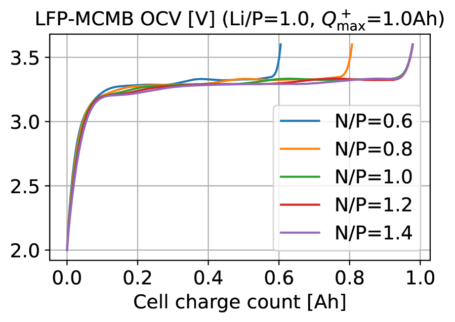
(a) $U_{\mathrm{OCV}}(Q_{\mathrm{c}};r_{\mathrm{N/P}},z^{+}_{0}=1,\hat{Q}_{\mathrm{max}}^{+}=1\mathrm{Ah})$

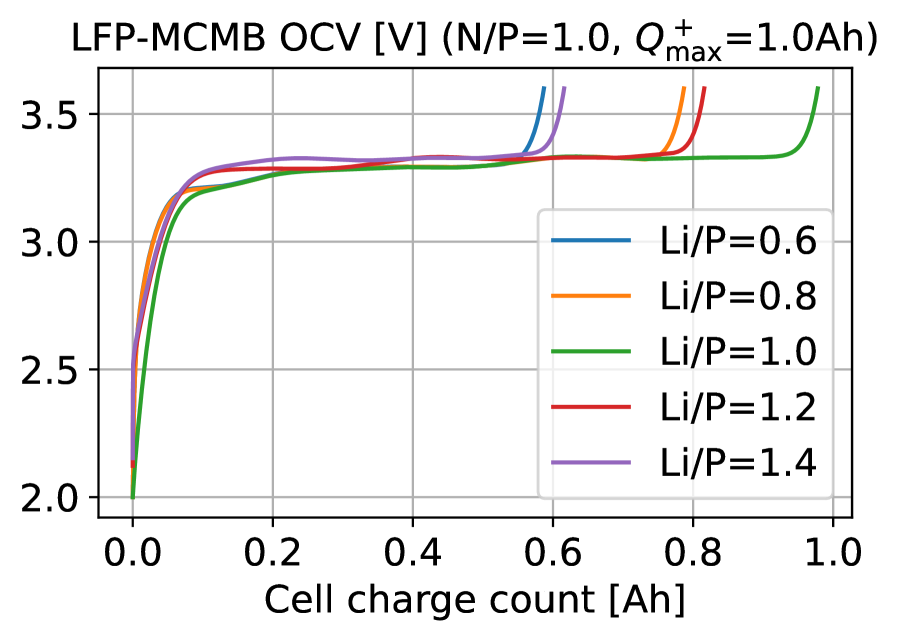
(b) $U_{\mathrm{OCV}}(Q_{\mathrm{c}};r_{\mathrm{N/P}}=1,z^{+}_{0},\hat{Q}_{\mathrm{max}}^{+}=1\mathrm{Ah})$

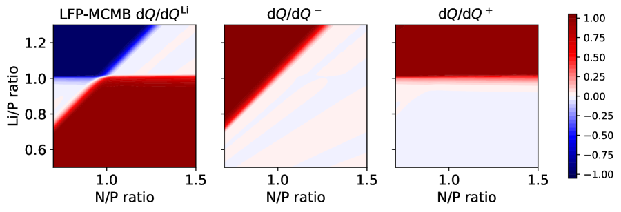
(c) $\mathrm{\partial}_{\hat{Q}_{\mathrm{max}}^{\mathrm{Li}}}\hat{Q}_{\mathrm{max}}$, $\mathrm{\partial}_{\hat{Q}_{\mathrm{max}}^{-}}\hat{Q}_{\mathrm{max}}$, and $\mathrm{\partial}_{\hat{Q}_{\mathrm{max}}^{+}}\hat{Q}_{\mathrm{max}}$

Figure 6: Top: Variation of $Q_{\mathrm{c}}$-based cell OCV and total capacity $\hat{Q}_{\mathrm{max}}$ when $r_{\mathrm{N/P}}$ changes and $z^{+}_{0}=1$ (top left) and when $z^{+}_{0}$ changes and $r_{\mathrm{N/P}}=1$ (top right), both assuming $\hat{Q}^{+}_{\mathrm{max}}=1\mathrm{Ah}$. For the former case, this implies that $\hat{Q}_{\mathrm{max}}^{-}$ changes while $\hat{Q}_{\mathrm{max}}^{\mathrm{Li}}=\hat{Q}^{+}_{\mathrm{max}}=1\mathrm{Ah}$. Bottom: Gradient-based sensitivity of total capacity with respect to the amount of lithium inventory, NE, and PE active materials at different $(r_{\mathrm{N/P}},z^{+}_{0})$ pairs.

Note that although $\hat{Q}_{\mathrm{max}}$ depends on all three of $\hat{Q}_{\mathrm{max}}^{\mathrm{Li}}$, $\hat{Q}_{\mathrm{max}}^{-}$, and $\hat{Q}_{\mathrm{max}}^{+}$, the dimensionless derivatives in (44) only depend on the also dimensionless $r_{\mathrm{N/P}}$ and $z^{+}_{0}$. Therefore, we can visualize the different regimes of a cell where the total capacity is limited by the three components to different extents by plotting the three profiles of $\mathrm{\partial}_{\hat{Q}_{\mathrm{max}}^{(\cdot)}}\hat{Q}_{\mathrm{max}}(r_{\mathrm{N/P}},z^{+}_{0})$ as shown in fig. 6. If we look at figs. 6 and 3 together, we can see how the four-quadrant pattern from $z^{\pm}_{\mathrm{min/max}}$ and $\lambda^{+}_{\mathrm{l/u}}$ propagates into $\mathrm{\partial}_{\hat{Q}_{\mathrm{max}}^{(\cdot)}}\hat{Q}_{\mathrm{max}}$ through (44). The characteristics of the four SOH regimes are summarized in table 1.

	Li $>$ N	Li $<$ N
	$\lambda^{-}_{\mathrm{u}}\rightarrow 1,\quad\mathrm{\partial}_{\hat{Q}_{\mathrm{max}}^{-}}\hat{Q}_{\mathrm{max}}\rightarrow 1$	$\lambda^{-}_{\mathrm{u}}\rightarrow 0,\quad\mathrm{\partial}_{\hat{Q}_{\mathrm{max}}^{-}}\hat{Q}_{\mathrm{max}}\rightarrow 0$
Li $>$ P	$\hat{Q}_{\mathrm{max}}^{\mathrm{Li}}>\hat{Q}_{\mathrm{max}}^{\pm}$	$\hat{Q}_{\mathrm{max}}^{-}>\hat{Q}_{\mathrm{max}}^{\mathrm{Li}}>\hat{Q}_{\mathrm{max}}^{+}$
$\lambda^{+}_{\mathrm{l}}\rightarrow 1,\quad\mathrm{\partial}_{\hat{Q}_{\mathrm{max}}^{+}}\hat{Q}_{\mathrm{max}}\rightarrow 1$	$\mathrm{\partial}_{\hat{Q}_{\mathrm{max}}^{\mathrm{Li}}}\hat{Q}_{\mathrm{max}}\rightarrow-1$	$\mathrm{\partial}_{\hat{Q}_{\mathrm{max}}^{\mathrm{Li}}}\hat{Q}_{\mathrm{max}}\rightarrow 0$
Li $<$ P	$\hat{Q}_{\mathrm{max}}^{+}>\hat{Q}_{\mathrm{max}}^{\mathrm{Li}}>\hat{Q}_{\mathrm{max}}^{-}$	$\hat{Q}_{\mathrm{max}}^{\mathrm{Li}}<\hat{Q}_{\mathrm{max}}^{\pm}$
$\lambda^{+}_{\mathrm{l}}\rightarrow 0,\quad\mathrm{\partial}_{\hat{Q}_{\mathrm{max}}^{+}}\hat{Q}_{\mathrm{max}}\rightarrow 0$	$\mathrm{\partial}_{\hat{Q}_{\mathrm{max}}^{\mathrm{Li}}}\hat{Q}_{\mathrm{max}}\rightarrow 0$	$\mathrm{\partial}_{\hat{Q}_{\mathrm{max}}^{\mathrm{Li}}}\hat{Q}_{\mathrm{max}}\rightarrow 1$

Table 1: Four regimes of sensitivity of cell total capacity $\hat{Q}_{\mathrm{max}}$ to lithium inventory $\hat{Q}_{\mathrm{max}}^{\mathrm{Li}}$ and active materials $\hat{Q}_{\mathrm{max}}^{\pm}$ divided by the relative amount between $\hat{Q}_{\mathrm{max}}^{\mathrm{Li}}$ and $\hat{Q}_{\mathrm{max}}^{-}$ (Li/N) and between $\hat{Q}_{\mathrm{max}}^{\mathrm{Li}}$ and $\hat{Q}_{\mathrm{max}}^{+}$ (Li/P). The Li/N ratio determines whether the end-of-charge is limited by NE filling up or PE being emptied, and $\hat{Q}_{\mathrm{max}}^{-}$ is only identifiable when NE is limiting end-of-charge. Likewise, the Li/P ratio determines whether the end-of-discharge is limited by PE filling up or NE being emptied, and $\hat{Q}_{\mathrm{max}}^{+}$ is only identifiable when PE is limiting end-of-discharge. In contrast, $\hat{Q}_{\mathrm{max}}^{\mathrm{Li}}$ is only identifiable when the two ratio are both larger or smaller than 1, where the surplus and lack of lithium become the capacity bottleneck, respectively.

On the other hand, the other parametrization $\hat{Q}_{\mathrm{max}}(r_{\mathrm{N/P}},z^{+}_{0},\hat{Q}_{\mathrm{max}}^{+})$ is not without advantage. We know the $z$-based cell OCV $U_{\mathrm{OCV}}(z)$ depends on $r_{\mathrm{N/P}}$ and $z^{+}_{0}$ only, and $\hat{Q}^{+}_{\mathrm{max}}$ only comes into the picture when the cell total capacity $\hat{Q}_{\mathrm{max}}$ is concerned. Therefore, the original parametrization confines all the dimensional contributions to $\hat{Q}_{\mathrm{max}}$ within the single $\hat{Q}^{+}_{\mathrm{max}}$, which is structurally more aligned with the underlying parametric dependence.

3 Applications of Analytic Identifiability

3.1 Evaluating Parameter Identifiability from OCV Measurements by Fisher Information

One immediate application of the sensitivity gradients is to quantify the minimal estimation errors in the latent SOH parameters from noisy voltage measurements. The simple idea is if we measure $y=f(\theta)$ with standard error $\sigma_{y}$ to estimate $\theta$, and we know $\theta$ and $y$ are close to some $\theta_{0}$ and $y_{0}=f(\theta_{0})$, respectively, we can linearize $f(\theta)$ around $\theta_{0}$ and thus $\sigma_{y}/\sigma_{\theta}=\mathrm{d}_{\theta}f(\theta_{0})$, which yields a standard error $\sigma_{\theta}=\sigma_{y}/\mathrm{d}_{\theta}f(\theta_{0})$. When this is generalized to the vector case with $m$ measurements $\bm{y}=\bm{f}(\bm{\theta})\in\mathbb{R}^{m}$ and $d$ underlying parameters $\bm{\theta}\in\mathbb{R}^{d}$, the derivative becomes the Jacobi matrix $\nabla_{\bm{\theta}}\bm{f}\in\mathbb{R}^{m\times d}$ and the $\sigma_{\bm{y}}^{2}$ and $\sigma_{\theta}^{2}$ become the error covariance $\bm{C}_{\bm{y}}\in\mathbb{R}^{m\times m}$ and $\bm{C}_{\bm{\theta}}\in\mathbb{R}^{d\times d}$, respectively. Aided by a square root of the symmetric positive definite $\bm{C}_{\bm{y}}$, we can obtain the vector counterpart of $\sigma_{\theta}=\sigma_{y}/\mathrm{d}_{\theta}f(\theta_{0})$ as

$$\bm{C}_{\bm{\theta}}^{-1}(\bm{\theta}_{0})=\nabla_{\bm{\theta}}^{\mathrm{T}}\bm{f}(\bm{\theta}_{0})\bm{C}_{\bm{y}}^{-1}\nabla_{\bm{\theta}}\bm{f}(\bm{\theta}_{0}).$$ (46)

If we solve the weighted NLS (nonlinear least squares) to obtain

$$\theta_{*}(\hat{\bm{y}})=\operatorname*{arg\,min}_{\bm{\theta}}(\bm{f}(\bm{\theta})-\hat{\bm{y}})^{\mathrm{T}}\bm{C}_{\bm{y}}^{-1}(\bm{f}(\bm{\theta})-\hat{\bm{y}}),$$ (47)

where $\hat{\bm{y}}$ are actual measured values of $\bm{y}$, substituting $\bm{\theta}_{*}$ to $\bm{\theta}_{0}$ in (46) yields a standard error covariance for the optimizer $\bm{\theta}_{*}$. Note, however, that such gradient-based identifiability results are only valid locally and are based on the premise that $\bm{\theta}_{*}$ is near the ground truth $\bm{\theta}_{\mathrm{tr}}$ and $\hat{\bm{y}}$ are noisy unbiased measurements of $\bm{f}(\bm{\theta}_{\mathrm{tr}})$ with covariance $\bm{C}_{\bm{y}}$. If the nonlinear optimization does not ever get close to $\bm{\theta}_{\mathrm{tr}}$, of course the above results are irrelevant to how close $\bm{\theta}_{*}$ is to $\bm{\theta}_{\mathrm{tr}}$.

When the weighted NLS optimizer $\bm{\theta}_{*}$ is equivalently formulated as the maximum likelihood estimator $\bm{\theta}_{*}(\hat{\bm{y}})=\operatorname*{arg\,max}_{\bm{\theta}}p(\hat{\bm{y}}|\bm{\theta})$ with a Gaussian likelihood $\bm{y}|\bm{\theta}\sim\mathcal{N}(\bm{f}(\bm{\theta}),\bm{C}_{\bm{y}})$, (46) turns out to be the well known Fisher information matrix [20]

$$\bm{F}_{\bm{y}}(\theta_{*})=\mathbb{E}_{\bm{y}|\bm{\theta}_{*}}[\nabla_{\bm{\theta}}^{\mathrm{T}}\ln p(\bm{y}|\bm{\theta_{*}})\nabla_{\bm{\theta}}\ln p(\bm{y}|\bm{\theta_{*}})]=\nabla_{\bm{\theta}}^{\mathrm{T}}\bm{f}(\bm{\theta}_{*})\bm{C}_{\bm{y}}^{-1}\nabla_{\bm{\theta}}\bm{f}(\bm{\theta}_{*}).$$ (48)

Under this probabilistic framework, the inverse Fisher information matrix is the Cramér-Rao lower bound of the covariance of all unbiased estimator $\hat{\bm{\theta}}(\hat{y})$, i.e. $(\mathrm{Cov}(\hat{\bm{\theta}}(\hat{y}))-\bm{F}_{\bm{y}}^{-1}(\theta_{\mathrm{tr}}))$ is semi-positive definite [21, sec. 11.10]. Although we do not know $\theta_{\mathrm{tr}}$ in practice, and the maximum likelihood estimator $\bm{\theta}_{*}(\hat{\bm{y}})$ is not necessarily unbiased, we can still use the inverse of (48) as a semi-heuristic error covariance, as [11, 15] have done for their OCV model parametrization (3). Due to the cutoff-voltage constraint between the two electrode SOC limits in their parameters, extra treatments are needed to evaluate the Fisher information matrix. The independent and cutoff-voltage-agnostic parametrization introduced in this work allows this to be done with more ease.

In practice, we can usually assume that the errors in different measurements are independent, which translates to $\bm{C}_{\bm{y}}=\mathrm{Diag}(\sigma_{y_{i}}^{2})$ being diagonal. In this case, the contributions of different measurements to $\bm{C}_{\bm{\theta}}^{-1}$ become additive rank-1 updates:

$$\bm{C}_{\bm{\theta}}^{-1}=\sum_{i=1}^{m}\frac{1}{\sigma_{y_{i}}^{2}}\nabla_{\bm{\theta}}^{\mathrm{T}}f_{i}(\bm{\theta}_{0})\nabla_{\bm{\theta}}f_{i}(\bm{\theta}_{0}).$$ (49)

If a complete OCV curve has been observed, naturally the total capacity $\hat{Q}_{\mathrm{max}}$ is also directly measured by Coulomb counting. What remains to be done is identifying the N/P and Li/P ratio $\bm{\theta}=[r_{\mathrm{N/P}},z^{+}_{0}]$ from the $(z_{i},\hat{U}_{i})$ pairs. Assume $z_{i}$ is accurate and every $\hat{U}_{i}$ has a standard error $\sigma_{U}$. Since $f_{i}(\theta)=U_{\mathrm{OCV}}(z_{i};r_{\mathrm{N/P}},z^{+}_{0})$ here, we have

$$\nabla_{\bm{\theta}}U_{\mathrm{OCV}}(z_{i})=[\mathrm{\partial}_{r_{\mathrm{N/P}}}U_{\mathrm{OCV}}(z_{i}),\mathrm{\partial}_{z^{+}_{0}}U_{\mathrm{OCV}}(z_{i})],$$ (50)

which together with (49) evaluated at the NLS optimizer $\bm{\theta}_{*}$ yields error covariance for $[r_{\mathrm{N/P}},z^{+}_{0}]$.

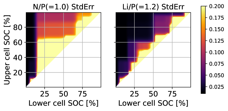
(a) $r_{\mathrm{N/P}}=1$ and $z^{+}_{0}=1.2$

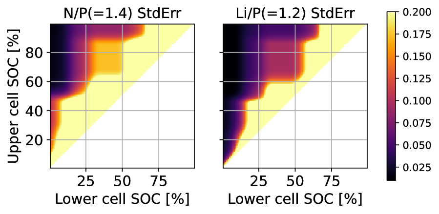
(b) $r_{\mathrm{N/P}}=1.4$ and $z^{+}_{0}=1.2$

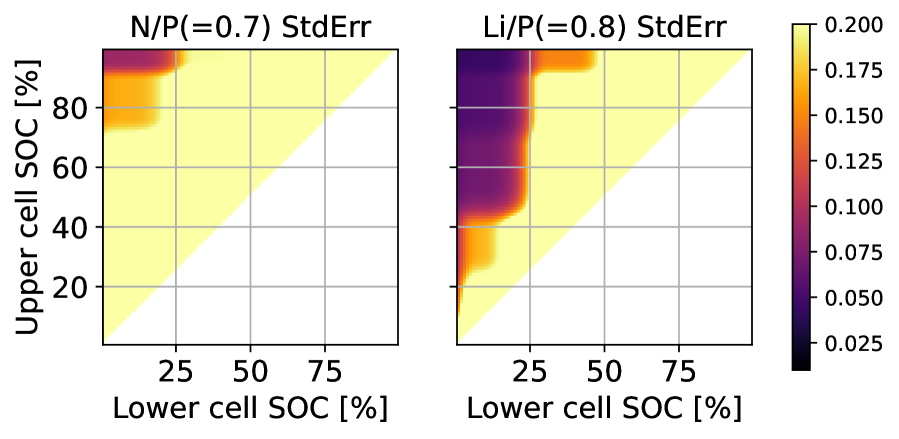
(c) $r_{\mathrm{N/P}}=0.7$ and $z^{+}_{0}=0.8$

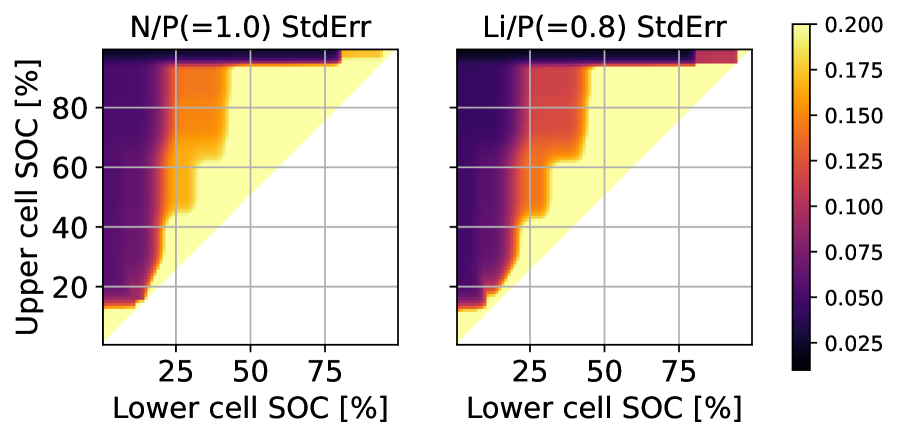
(d) $r_{\mathrm{N/P}}=1$ and $z^{+}_{0}=0.8$

Figure 7: Standard estimation errors of the N/P ratio $r_{\mathrm{N/P}}$ and Li/P ratio $z^{+}_{0}$ based on OCV measurements sampled at every $1\%$ SOC within any cell SOC window $[z_{\mathrm{lower}},z_{\mathrm{upper}}]$ at least $1\%$ apart. The errors are obtained as the square root of the diagonals of the inverse Fisher information matrix evaluated at different pairs of $(r_{\mathrm{N/P}},z^{+}_{0})$ values. The standard OCV measurement error is assumed to be $\sigma_{U}=5\mathrm{mV}$.

The above results are applied to the same LFP-graphite chemistry as used before with four different $(r_{\mathrm{N/P}},z^{+}_{0})$ pairs to examine how informative OCV measurements from certain SOC windows are about the N/P ratio $r_{\mathrm{N/P}}$ and Li/P ratio $z^{+}_{0}$, as shown in fig. 7. We choose the OCV at SOC $z=1\%,2\%,\ldots,99\%$ as candidate measurements and traverse every SOC window $[z_{\mathrm{lower}},z_{\mathrm{upper}}]$ with ends from them that contains at least two measurements. The standard error of OCV measurements is assumed to be $\sigma_{U}=5\mathrm{mV}$, and the standard estimation errors of $r_{\mathrm{N/P}}$ and $z^{+}_{0}$ for each SOC window obtained by the square root of $\mathrm{diag}(\bm{C}_{\bm{\theta}})$ are demonstrated in each sub-figure of fig. 7. We limit the color bar to the range of $[0.01,0.2]$ to visualize the practically relevant features, because a standard error larger than $0.2$ for $r_{\mathrm{N/P}}$ and $z^{+}_{0}$ having a value around 1 means the estimation is almost useless. On the other hand, the OCV model is not perfect in practice, and model errors will limit the estimation accuracy in the first place, so we consider an estimation error of under $0.01$ in this ideal setup as more than enough. Hence, in fig. 7, a dark zone indicates small-enough errors while a bright zone implies ineffective estimation.

Note that if one SOC window is nested in another, the OCV measurements of the latter also contain all those in the former, so the estimation error is monotonically decreasing vertically and increasing horizontally. Moreover, we see the errors having a sharp change in certain SOC, indicating the OCV measurements at such SOC to be particularly sensitive to $r_{\mathrm{N/P}}$ and $z^{+}_{0}$, agreeing with figs. 4(d) and 5(d). We can also observe that estimating $r_{\mathrm{N/P}}$ is harder than estimating $z^{+}_{0}$ in this case, which is consistent with fig. 2(b), and OCV values at low SOC are overall more informative than those at high SOC.

3.2 Interpreting Incremental Capacity Fade: Relating LLI and LAM to Coulombic Efficiency and Capacity Retention

In practice, we are not only interested in the current extent of capacity fade, but also concerned with the speed of capacity fade, which can help us project the life span of a cell. The speed of capacity fade is usually estimated by cycling a cell within a certain SOC window under the same protocol and counting the charge throughput during each charging and discharging step with high-precision coulometry to monitor their minute differences [17]. The SOC window is usually specified by the upper and lower cutoff voltage and the cell is ensured to reach them at the end of charging and discharging by either cycling at a very small C-rate (e.g. 0.05C) or attaching a CV (constant-voltage) phase at the corresponding cutoff voltage to the end of both charging and discharging with a small cutoff current. Since the incremental capacity loss is typically small for a well-manufactured and properly functioning cell, we can use the sensitivity derivatives derived previously for a cell OCV curve under a rigorous first-order analysis framework to relate the observable metrics regarding the speed of capacity fade to the underlying rates of LLI and LAM.

Suppose a cell is initially fully discharged (i.e. $U_{\mathrm{OCV}}=U_{\mathrm{min}}$) and undergoes the following two charge-discharge cycles:

$$\mathrm{D}_{0}\xrightarrow{Q_{\mathrm{c1}}}\mathrm{C}_{1}\xrightarrow{Q_{\mathrm{d1}}}\mathrm{D}_{1}\xrightarrow{Q_{\mathrm{c2}}}\mathrm{C}_{2}\xrightarrow{Q_{\mathrm{d2}}}\mathrm{D}_{2},$$ (51)

where $\mathrm{D}_{i}$ and $\mathrm{C}_{i}$ denote the cell state at the end of $i$-th discharging and charging, respectively, while $Q_{\mathrm{d}i}$ and $Q_{\mathrm{c}i}$ refer to the $i$-th discharge and charge capacity, respectively, measured by the Coulomb counting. With these capacity measurements, we can define the Coulombic efficiency and capacity retention as

$$\eta=\frac{Q_{\mathrm{d1}}}{Q_{\mathrm{c1}}},\qquad\mathrm{CR}=\frac{Q_{\mathrm{d2}}}{Q_{\mathrm{d1}}}.$$ (52)

Of course, this is not the only way to define them, and we will discuss later the subtle implications of using alternative definitions.

Typically, both $\eta$ and $\mathrm{CR}$ are smaller than but very close to $1$ due to slow cycle aging, i.e.

$$0<1-\eta\ll 1,\qquad 0<1-\mathrm{CR}\ll 1,$$ (53)

unless in anomalous cases where the cell has somehow not yet reached reasonable equilibrium in the end of charging or discharging [22]. In particular, $\eta<1$ implies that the charge capacity $Q_{\mathrm{c1}}$ is larger than the discharge capacity $Q_{\mathrm{d1}}$, which has been primarily attributed to the reductive side reactions competing with lithium intercalation at the NE during charging, of which the SEI (solid-electrolyte interface) layer growth and lithium plating are considered the major mechanisms. Since such side reactions do not (fully) revert during lithium disintercalation at the NE in discharging, the charge throughput difference associated with these side reactions manifest itself in the aggregate count. Meanwhile, some lithium ions will be permanently consumed and no longer able to participate in cycling, hence contributing to LLI. On the other hand, any incremental LLI or LAM will typically reduce the discharge capacity from cycle to cycle, so $\mathrm{CR}<1$ is quite straightforward.

Next, we will define the underlying rates of LLI and LAM in cycle aging that cause the observed $\eta<1$ and $\mathrm{CR}<1$. Since kinetic effects including side reaction rates are often not symmetric between charging and discharging, we define the rates of LLI and LAM separately for these two cases. First, we quantify the rate of LLI by the electrode Coulombic efficiency defined as the fraction of charges passing through the electrode that translate to the changes of cyclable lithium stored in the electrode:

$$\mathrm{Charging:}\quad\eta_{\mathrm{red}}^{-}=\frac{\Delta\hat{Q}^{-}}{Q_{\mathrm{c}}},\quad\eta_{\mathrm{ox}}^{+}=\frac{-\Delta\hat{Q}^{+}}{Q_{\mathrm{c}}};$$ (54)

$$\mathrm{Discharging:}\quad\eta_{\mathrm{ox}}^{-}=\frac{-\Delta\hat{Q}^{-}}{Q_{\mathrm{d}}},\quad\eta_{\mathrm{red}}^{+}=\frac{\Delta\hat{Q}^{+}}{Q_{\mathrm{d}}},$$ (55)

where $\Delta\hat{Q}^{\pm}$ denotes the change of $\hat{Q}^{\pm}$ from the beginning to the end of charging/discharging, recalling that $\hat{Q}^{\pm}=z^{\pm}\hat{Q}_{\mathrm{max}}^{\pm}$ is the instantaneous amount of cyclable lithium in an electrode.

Note that with LLI and LAM continuously taking place, although operating parameters such as the upper and lower cutoff voltage can be fixed, the SOH parameters $\hat{Q}_{\mathrm{max}}^{\pm}$ and $\hat{Q}_{\mathrm{max}}^{\mathrm{Li}}$, and consequently $z^{\pm}_{\mathrm{max}}$ and $z^{\pm}_{\mathrm{min}}$, are constantly varying, so their values at each of $\mathrm{D}_{i}$ and $\mathrm{C}_{i}$ can be different. Another subtlety lies in that the electrode Coulombic efficiency defined above not only accounts for electrochemical side reactions as conventionally implied by the term, but is also affected by any degradation mechanism that can alter the total amount of cyclable lithium in the electrode, such as particle cracking, electrolyte dry-out, and electric contact loss, which can all cause certain active materials that might be partially lithiated to become permanently isolated, forming some dead zones and contributing to both LAM and LLI.

Also note that the above definitions entail that if side reactions are the major culprit of LLI, the $\eta^{\pm}$’s are less than $1$ when side reactions are in the same redox direction as the main ones, i.e. reductive during lithium intercalation and oxidative during disintercalation, as is usually the case, but of course, this is just a sign convention and does not preclude the possibility of $\eta^{\pm}>1$. Moreover, side reactions do not necessarily reduce cyclable lithium. Indeed, only reductive side reactions do so while to the opposite, oxidative ones increase cyclable lithium, because some lithium supposed to be disintercalated do not have to now and can remain in the electrode thanks to other oxidative reactions that share the oxidative current.

The electrode Coulombic efficiency $\eta^{\pm}$’s defined as eq. 54 are quantities averaged over the whole charging/discharging half cycle. Of course, we can also define their instantaneous counterparts such as

$$\eta_{\mathrm{red}}^{-}=\frac{\mathrm{d}\hat{Q}^{-}}{\mathrm{\delta}Q_{\mathrm{c}}}=\frac{\mathrm{d}_{t}\hat{Q}^{-}}{I_{\mathrm{c}}}=\frac{\mathrm{d}_{t}\hat{Q}^{-}}{I_{\mathrm{red}}^{-}},\qquad\eta_{\mathrm{ox}}^{+}=\frac{-\mathrm{d}\hat{Q}^{+}}{\mathrm{\delta}Q_{\mathrm{c}}}=\frac{-\mathrm{d}_{t}\hat{Q}^{+}}{I_{\mathrm{c}}}=\frac{\mathrm{d}_{t}\hat{Q}^{+}}{I_{\mathrm{red}}^{+}},$$ (56)

which can be unified as

$$\eta^{\pm}=\frac{\mathrm{d}\hat{Q}^{\pm}}{\mathrm{\delta}Q_{\mathrm{red}}^{\pm}}=\frac{\mathrm{d}_{t}\hat{Q}^{\pm}}{I_{\mathrm{red}}^{\pm}}$$ (57)

for both electrodes and for both charging and discharging. Here $I_{\mathrm{red}}^{\pm}$ and $\mathrm{\delta}Q_{\mathrm{red}}^{\pm}$ denote the electrode current and incremental electrode charge throughput, respectively, both measured in the reductive direction so $I_{\mathrm{red}}^{+}=-I_{\mathrm{red}}^{-}$ and $\mathrm{\delta}Q_{\mathrm{red}}^{+}=-\mathrm{\delta}Q_{\mathrm{red}}^{-}$. These instantaneous $\eta^{\pm}$’s are not likely constants and will typically vary significantly across different electrode SOC and current. For example, lithium plating at the NE is known to be much more severe at high NE SOC during fast charging. Due to such variability and the limited granularity of our half-cycle analysis setup (51), we adopt the half-cycle-averaged definitions (54) as metrics for the LLI rate.

Last but not least, since our subsequent first-order analysis concerns the small quantities $(1-\eta^{\pm})$ much more than the $\eta^{\pm}$’s themselves, we introduce the following trivial definition of electrode Coulombic inefficiency for notational convenience:

$$\beta^{\pm}_{\mathrm{red}}=1-\eta^{\pm}_{\mathrm{red}},\qquad\beta^{\pm}_{\mathrm{ox}}=1-\eta^{\pm}_{\mathrm{ox}}.$$ (58)

In contrast to the case of LLI, the definitions of LAM rates are much more straightforward:

$$\mathrm{Charging:}\quad\alpha_{\mathrm{red}}^{-}=\frac{-\Delta\hat{Q}_{\mathrm{max}}^{-}}{Q_{\mathrm{c}}},\quad\alpha_{\mathrm{ox}}^{+}=\frac{-\Delta\hat{Q}_{\mathrm{max}}^{+}}{Q_{\mathrm{c}}};$$ (59)

$$\mathrm{Discharging:}\quad\alpha_{\mathrm{ox}}^{-}=\frac{-\Delta\hat{Q}_{\mathrm{max}}^{-}}{Q_{\mathrm{d}}},\quad\alpha_{\mathrm{red}}^{+}=\frac{-\Delta\hat{Q}_{\mathrm{max}}^{+}}{Q_{\mathrm{d}}}.$$ (60)

As has been mentioned, we typically have

$$0<\alpha_{\mathrm{red}}^{\pm},~{}\alpha_{\mathrm{ox}}^{\pm}\ll 1.$$ (61)

Inspired by the form of eqs. 59 and 60, we can also define their counterpart for lithium inventory $\hat{Q}_{\mathrm{max}}^{\mathrm{Li}}$ and relate it to the previously defined electrode Coulombic efficiency:

$$\alpha_{\mathrm{c}}^{\mathrm{Li}}=\frac{-\Delta\hat{Q}_{\mathrm{max}}^{\mathrm{Li}}}{Q_{\mathrm{c}}}=\frac{-(\Delta\hat{Q}^{+}+\Delta\hat{Q}^{-})}{Q_{\mathrm{c}}}=\eta_{\mathrm{ox}}^{+}-\eta_{\mathrm{red}}^{-}=\beta_{\mathrm{red}}^{-}-\beta_{\mathrm{ox}}^{+},$$ (62)

$$\alpha_{\mathrm{d}}^{\mathrm{Li}}=\frac{-\Delta\hat{Q}_{\mathrm{max}}^{\mathrm{Li}}}{Q_{\mathrm{d}}}=\frac{-(\Delta\hat{Q}^{+}+\Delta\hat{Q}^{-})}{Q_{\mathrm{d}}}=\eta_{\mathrm{ox}}^{-}-\eta_{\mathrm{red}}^{+}=\beta_{\mathrm{red}}^{+}-\beta_{\mathrm{ox}}^{-}.$$ (63)

Note how the rightmost two expressions clearly encode the opposite contributions of reductive and oxidative side reactions to LLI. It turns out that the $\eta^{\pm}$’s will frequently enter our subsequent analysis through $\alpha_{\mathrm{c}}^{\mathrm{Li}}$ and $\alpha_{\mathrm{d}}^{\mathrm{Li}}$.

With the various metrics for the rates of LAM and LLI precisely defined, we can proceed to relate them to the observed Coulombic efficiency $\eta$ and capacity retention $\mathrm{CR}$. The first step is to relate the observed charge and discharge capacity to the underlying cell total capacity. Suppose charging and discharging are ensured to traverse the whole range between the fully discharged and charged state. When there is no LAM or LLI, all three of charge, discharge, and total capacity should coincide. Now if there is some slow cycle aging characterized by

$$|\beta^{\pm}_{\mathrm{red}}|,~{}|\beta^{\pm}_{\mathrm{ox}}|,~{}|\alpha^{\pm}_{\mathrm{red}}|,~{}|\alpha^{\pm}_{\mathrm{ox}}|\ll 1,$$ (64)

the charge and discharge capacity shall slightly deviate from the total capacity. Besides, the total capacity itself will also have a small discrepancy before and after charging/discharging. Up to first-order approximation, these deviations is linear in the $\alpha^{\pm}$’s and $\beta^{\pm}$’s, and since aging is slow, this linear approximation should be a good characterization of the aging.

By calculating the small changes of $\hat{Q}_{\mathrm{max}}^{\mathrm{Li}}$ and $\hat{Q}_{\mathrm{max}}^{\pm}$ based on the LLI and LAM rates, we can use the previously obtained derivatives with respect to them to express the small changes in all other quantities in terms of the LLI and LAM rates (derivation details in Support Information). In particular, we can obtain the cell Coulombic efficiency as

$$\eta_{\mathrm{c,d}}=\frac{Q_{\mathrm{d1}}}{Q_{\mathrm{c1}}}\approx\frac{1+\beta_{\mathrm{ox}}^{-}\lambda^{-}_{\mathrm{l}}+\beta_{\mathrm{red}}^{+}\lambda^{+}_{\mathrm{l}}+\alpha_{\mathrm{ox}}^{-}z^{-}_{\mathrm{min}}\lambda^{-}_{\mathrm{l}}-\alpha_{\mathrm{red}}^{+}z^{+}_{\mathrm{max}}\lambda^{+}_{\mathrm{l}}}{1+\beta_{\mathrm{red}}^{-}\lambda^{-}_{\mathrm{l}}+\beta_{\mathrm{ox}}^{+}\lambda^{+}_{\mathrm{l}}-\alpha_{\mathrm{red}}^{-}z^{-}_{\mathrm{min}}\lambda^{-}_{\mathrm{l}}+\alpha_{\mathrm{ox}}^{+}z^{+}_{\mathrm{max}}\lambda^{+}_{\mathrm{l}}},$$ (65)

where the subscript of $\eta_{\mathrm{c,d}}$ indicates that in this definition of $\eta$, the charge step precedes the discharge one. With further first-order approximation, the above reduces to

$$\eta_{\mathrm{c,d}}\approx 1-(\beta_{\mathrm{red}}^{-}-\beta_{\mathrm{ox}}^{-})\lambda^{-}_{\mathrm{l}}-(\beta_{\mathrm{ox}}^{+}-\beta_{\mathrm{red}}^{+})\lambda^{+}_{\mathrm{l}}+(\alpha_{\mathrm{red}}^{-}+\alpha_{\mathrm{ox}}^{-})z^{-}_{\mathrm{min}}\lambda^{-}_{\mathrm{l}}-(\alpha_{\mathrm{ox}}^{+}+\alpha_{\mathrm{red}}^{+})z^{+}_{\mathrm{max}}\lambda^{+}_{\mathrm{l}}.$$ (66)

First, let us verify that the signs are aligned with our physical intuition. Since cathode LAM delays charging but hastens discharging, both $\alpha_{\mathrm{ox}}^{+}$ and $\alpha_{\mathrm{red}}^{+}$ tend to reduce $\eta_{\mathrm{c,d}}$. In contrary, anode LAM hastens charging while delays discharging, so both $\alpha_{\mathrm{red}}^{-}$ and $\alpha_{\mathrm{ox}}^{-}$ contribute positively. On the other hand, side reactions competing with the lithium (dis)intercalation happening at the same electrode always delay reaching the end of charge/discharge, so side reactions during charging associated with $\beta_{\mathrm{red}}^{-}$ and $\beta_{\mathrm{ox}}^{+}$ increase charge capacity and thus decrease $\eta_{\mathrm{c,d}}$, while those during discharging have the opposite effect.

Second, eq. 66 implies that the side reactions or LAM processes during charging and discharging affect the Coulombic efficiency only in an aggregate manner under first-order approximation. In other words, the contribution of each aging process during charging and that during discharging are indistinguishable. Therefore, if we define the overall charge-discharge average rate for each $\alpha^{\pm}$ and $\beta^{\pm}$ as

$$\bar{\beta}_{\mathrm{red}}^{-}=\frac{\beta_{\mathrm{red}}^{-}-\beta_{\mathrm{ox}}^{-}}{2},\quad\bar{\beta}_{\mathrm{ox}}^{+}=\frac{\beta_{\mathrm{ox}}^{+}-\beta_{\mathrm{red}}^{+}}{2},\quad\bar{\alpha}^{-}=\frac{\alpha_{\mathrm{red}}^{-}+\alpha_{\mathrm{ox}}^{-}}{2},\quad\bar{\alpha}^{+}=\frac{\alpha_{\mathrm{ox}}^{+}+\alpha_{\mathrm{red}}^{+}}{2},$$ (67)

eq. 66 can be simplified to

$$\eta_{\mathrm{c,d}}\approx 1-2(\bar{\beta}_{\mathrm{red}}^{-}-\bar{\alpha}^{-}z^{-}_{\mathrm{min}})\lambda^{-}_{\mathrm{l}}-2(\bar{\beta}_{\mathrm{ox}}^{+}+\bar{\alpha}^{+}z^{+}_{\mathrm{max}})\lambda^{+}_{\mathrm{l}}.$$ (68)

Note that when averaging the electrode side reaction rates $\beta^{\pm}$, we must specify whether reduction or oxidation is used as the positive direction. Since side reactions are usually much more prominent during charging, we assume that the NE side reactions are overall reductive while the PE ones oxidative.

One ostensible caveat of approximating (65) by (66) is losing the distinguishability between charge and discharge aging, because the two indeed contribute to $\eta_{\mathrm{c,d}}$ differently according to (65). However, this distinguishability is only a higher-order effect and keep in mind that several first-order approximations have been made to obtain (65) in the first place, which renders any seemingly remaining higher-order effects mere artifacts of a particular path of derivation. For example, [16] generalizes [19]’s result of the dependence of Coulombic efficiency on side reaction rates. Under our framework and notations, they have assumed $\alpha^{\pm}_{\mathrm{red}}=\alpha^{\pm}_{\mathrm{ox}}=0$, which according to (65), should yield

$$\eta_{\mathrm{c,d}}\approx\frac{1+\beta_{\mathrm{ox}}^{-}\lambda^{-}_{\mathrm{l}}+\beta_{\mathrm{red}}^{+}\lambda^{+}_{\mathrm{l}}}{1+\beta_{\mathrm{red}}^{-}\lambda^{-}_{\mathrm{l}}+\beta_{\mathrm{ox}}^{+}\lambda^{+}_{\mathrm{l}}}.$$

This is essentially equation (9) in [16], which should have been reduced to

$$\eta_{\mathrm{c,d}}\approx 1-(\beta_{\mathrm{red}}^{-}-\beta_{\mathrm{ox}}^{-})\lambda^{-}_{\mathrm{l}}-(\beta_{\mathrm{ox}}^{+}-\beta_{\mathrm{red}}^{+})\lambda^{+}_{\mathrm{l}}.$$ (69)

In the majority of their paper, they have further assumed

$$\bar{\beta}_{\mathrm{red}}^{-}=\beta_{\mathrm{red}}^{-}=-\beta_{\mathrm{ox}}^{-},\quad\bar{\beta}_{\mathrm{ox}}^{+}=\beta_{\mathrm{ox}}^{+}=-\beta_{\mathrm{red}}^{+},$$

which simplifies the Coulombic efficiency to

$$\eta_{\mathrm{c,d}}\approx\frac{1-\bar{\beta}_{\mathrm{red}}^{-}\lambda^{-}_{\mathrm{l}}-\bar{\beta}_{\mathrm{ox}}^{+}\lambda^{+}_{\mathrm{l}}}{1+\bar{\beta}_{\mathrm{red}}^{-}\lambda^{-}_{\mathrm{l}}+\bar{\beta}_{\mathrm{ox}}^{+}\lambda^{+}_{\mathrm{l}}},$$

and is essentially equation (1) in [16]. Likewise, this should have been further simplified to

$$\eta_{\mathrm{c,d}}\approx 1-2\bar{\beta}_{\mathrm{red}}^{-}\lambda^{-}_{\mathrm{l}}-2\bar{\beta}_{\mathrm{ox}}^{+}\lambda^{+}_{\mathrm{l}}.$$

The simulation results in [16] clearly show the linear dependence of $\eta_{\mathrm{c,d}}$ on $I_{\mathrm{red}}/I$ and $I_{\mathrm{ox}}/I$, which justifies using the above linear approximation. On the other hand, even if the side reactions are so significant that linear approximation is no longer adequate, the fractional form of (65) is still based on linear approximation and is not the exact solution, so it is inaccurate and unreliable, either. Hence, keeping the first-order approximation results in an intermediate seemingly nonlinear form simply retains not only unnecessary but also misleading complexity.

One last remark regarding Coulombic efficiency is that according to eq. 68, it depends only on the electrode DV fractions at the lower cutoff voltage but not those at the upper, i.e. $\lambda^{\pm}_{\mathrm{l}}$ but not $\lambda^{\pm}_{\mathrm{u}}$, which has also been pointed out by [16]. However, this turns out to be only an artifact of defining Coulombic efficiency conventionally based on a charge-discharge cycle, i.e. with the charge step preceding the discharge one. In principle, nothing stops us from quantifying the Coulombic efficiency instead by a discharge-charge cycle:

$$\eta_{\mathrm{d,c}}=\frac{Q_{\mathrm{c2}}}{Q_{\mathrm{d1}}}\approx 1-2(\bar{\beta}_{\mathrm{red}}^{-}-\bar{\alpha}^{-}z^{-}_{\mathrm{max}})\lambda^{-}_{\mathrm{u}}-2(\bar{\beta}_{\mathrm{ox}}^{+}+\bar{\alpha}^{+}z^{+}_{\mathrm{min}})\lambda^{+}_{\mathrm{u}}.$$ (70)

We can find that the above shares the same form as eq. 68 for $\eta_{\mathrm{c,d}}$, except with $\lambda^{\pm}_{\mathrm{l}}$ in the latter replaced by $\lambda^{\pm}_{\mathrm{u}}$, and the two end-of-discharge SOC limits switching to their end-of-charge counterparts, respectively. This pattern is also intuitive physically, because in a charge-discharge cycle, the fully charged state is shared by the two steps so the difference between charge and discharge capacity is solely due to the change of the fully-discharged state at the lower cutoff voltage. Hence, $\eta_{\mathrm{c,d}}$ depends only on quantities associated with the fully discharged state, while the opposite applies to $\eta_{\mathrm{d,c}}$.

Deriving eq. 70 for $\eta_{\mathrm{d,c}}$ also facilitates calculating the capacity retention since

$$\mathrm{CR}_{\mathrm{d}}=\frac{Q_{\mathrm{d2}}}{Q_{\mathrm{d1}}}=\left.\frac{Q_{\mathrm{d2}}}{Q_{\mathrm{c2}}}\middle/\frac{Q_{\mathrm{d1}}}{Q_{\mathrm{c2}}}\right.\approx\frac{\eta_{\mathrm{c,d}}}{\eta_{\mathrm{d,c}}}.$$ (71)

Therefore, substituting eqs. 68 and 70 into the above yields

$$\mathrm{CR}_{\mathrm{d}}\approx 1-2\bar{\alpha}^{\mathrm{Li}}(\lambda^{+}_{\mathrm{u}}-\lambda^{+}_{\mathrm{l}})-2\bar{\alpha}^{-}(z^{-}_{\mathrm{max}}\lambda^{-}_{\mathrm{u}}-z^{-}_{\mathrm{min}}\lambda^{-}_{\mathrm{l}})-2\bar{\alpha}^{+}(z^{+}_{\mathrm{max}}\lambda^{+}_{\mathrm{l}}-z^{+}_{\mathrm{min}}\lambda^{+}_{\mathrm{u}}).$$ (72)

We can similarly calculate $\mathrm{CR}_{\mathrm{c}}=Q_{\mathrm{c2}}/Q_{\mathrm{c1}}$ and find out that $\mathrm{CR}_{\mathrm{d}}\approx\mathrm{CR}_{\mathrm{c}}$. Therefore, when aging is slow and first-order approximation is concerned, we do not need to specify what capacity we are talking about regarding capacity retention across one cycle, because they are simply the same.

With eqs. 68, 70 and 72, we have obtained a complete first-order characterization of how the incremental capacity fade is manifested in Coulombic efficiency and capacity retention. Note that the conventional choice of examining $\eta_{\mathrm{c,d}}$ and $\mathrm{CR}$ yields exactly the same information from examining $\eta_{\mathrm{c,d}}$ and $\eta_{\mathrm{d,c}}$ instead. However, although $\mathrm{CR}$ of the former might be more intuitive, the latter is probably more amenable to analysis because $\mathrm{CR}$ involves parameters associated with both the fully charged and discharged state, while $\eta_{\mathrm{d,c}}$ and $\eta_{\mathrm{c,d}}$ depend on the two separately.

For example, if LAM is negligible compared to side reactions, we have

$$\eta_{\mathrm{c,d}}\approx 1-2\bar{\beta}_{\mathrm{red}}^{-}\lambda^{-}_{\mathrm{l}}-2\bar{\beta}_{\mathrm{ox}}^{+}\lambda^{+}_{\mathrm{l}},\qquad\eta_{\mathrm{d,c}}\approx 1-2\bar{\beta}_{\mathrm{red}}^{-}\lambda^{-}_{\mathrm{u}}-2\bar{\beta}_{\mathrm{ox}}^{+}\lambda^{+}_{\mathrm{u}}.$$ (73)

If the two are measured in two consecutive cycles, and we somehow also have access to the electrode SOC limits and DV fractions (e.g. by a reference electrode in a three-electrode setup), we can immediately solve for the two electrode side reaction rates unless $\lambda^{+}_{\mathrm{u}}\approx\lambda^{+}_{\mathrm{l}}$ (hence also $\lambda^{-}_{\mathrm{u}}\approx\lambda^{-}_{\mathrm{l}}$), which makes the linear system ill-conditioned. In the general case with LAM also present, we have four unknown aging rates and thus need four equations to solve for them. One possibility to obtain another two independent equations is to wait for a period of cell operation before measuring $\eta_{\mathrm{c,d}}$ and $\eta_{\mathrm{d,c}}$ again, when the electrode SOC limits and DV fractions might have gone through some appreciable changes upon a finite amount of LAM and LLI. Of course, we must assume that the aging rates remain more or less constant throughout for this calculation to make sense.

4 Conclusions, Discussions, and Future Work

In this work, we study the electrode-specific OCV model assembled from the PE and NE OCP and propose a minimal and intuitive parametrization based on the dimensionless N/P ratio $r_{\mathrm{N/P}}=\hat{Q}_{\mathrm{max}}^{-}/\hat{Q}_{\mathrm{max}}^{+}$ and the Li/P ratio $z^{+}_{0}=\hat{Q}_{\mathrm{max}}^{\mathrm{Li}}/\hat{Q}_{\mathrm{max}}^{+}$, which are independent, cutoff-voltage-agnostic, pristine-condition-agnostic, and intuitively linked to the lithium inventory $\hat{Q}_{\mathrm{max}}^{\mathrm{Li}}$ and active material amounts $\hat{Q}_{\mathrm{max}}^{\pm}$. Estimating them thus gives us important information about the degradation mode of LLI, LAMn, and LAMp. Along the way, we also clarify several confusions regarding electrode stoichiometry $x^{\pm}$ versus electrode SOC $z^{\pm}$, precise meaning of cell SOC $z$ and SOH, and their relations to the artificially specified upper and lower cutoff voltage.

We then analytically derive the sensitivity gradients of the electrode SOC limits and $z$-based cell OCV $U_{\mathrm{OCV}}(z)$ with respect to the N/P and Li/P ratio. Such analytic results not only offer a closed-form expression to easily calculate these derivatives, but the form of the expressions also provides insights into how each factor affects the parametric sensitivity. In particular, the concept of PE and NE DV fraction naturally emerges in the derivation, which characterize which electrode is dominating the OCV changes at each cell SOC and are instrumental in propagating the effects of a fixed upper and lower cutoff voltage into the sensitivity gradients. The local sensitivity delineated by these parametric derivatives are visualized and verified by simulations and comparison against empirical sensitivity results.

Furthermore, we derive the sensitivity gradients of cell total capacity $\hat{Q}_{\mathrm{max}}$ with respect to the lithium inventory $\hat{Q}_{\mathrm{max}}^{\mathrm{Li}}$ and active material amounts $\hat{Q}_{\mathrm{max}}^{\pm}$. These dimensionless derivatives intuitively indicate to what extent each degradation mode of LLI, LAMn, and LAMp is limiting the apparent total capacity. Visualizing the pattern of their dependence on the N/P and Li/P ratio reveals four characteristic regimes regarding their identifiability.

We also demonstrate two applications of these analytic results in practice. The first regards estimating the N/P and Li/P ratio from complete OCV curve measurements using NLS. We show how to obtain an NLS estimator error covariance from the Fisher information matrix, which directly depends on the sensitivity gradients, and how such information helps us choose an SOC window that yields informative OCV measurements. The second application concerns incremental degradation, where we show how the sensitivity gradients help us relate the observed Coulombic efficiency and capacity retention to the underlying LLI and LAM rate using rigorous first-order analysis. This clarifies and extends previous results, providing new insights into alternatives of these metrics.

We want to emphasize that any statements based on sensitivity gradients are only valid locally, i.e. valid for a small range of parameters around the point at which the gradients are evaluated. More empirical tools from statistical inference will be needed to discern global sensitivity, and we will report our findings in future work.

Another limitation is that we have only discussed inferring degradation modes from OCV measurements, which has a relatively restricted scope of application in practice. To go beyond OCV measurements, we need to somehow estimate the cell SOC or OCV from terminal voltage recorded in finite-current operation. This can either be done by simple $IR_{0}$ corrections based on equivalent internal resistance $R_{0}$ [23], or by more sophisticated model-based filtering such as in a battery management system [5].

References

- Edge et al. [2021] J. S. Edge, S. O’Kane, R. Prosser, N. D. Kirkaldy, A. N. Patel, A. Hales, A. Ghosh, W. Ai, J. Chen, J. Jiang, Lithium Ion Battery Degradation: What you need to know, Physical Chemistry Chemical Physics (2021). Publisher: Royal Society of Chemistry.
- Attia et al. [2022] P. M. Attia, A. Bills, F. B. Planella, P. Dechent, G. d. Reis, M. Dubarry, P. Gasper, R. Gilchrist, S. Greenbank, D. Howey, O. Liu, E. Khoo, Y. Preger, A. Soni, S. Sripad, A. G. Stefanopoulou, V. Sulzer, Review—“Knees” in Lithium-Ion Battery Aging Trajectories, Journal of The Electrochemical Society 169 (2022) 060517. URL: https://doi.org/10.1149/1945-7111/ac6d13. doi:10.1149/1945-7111/ac6d13, publisher: The Electrochemical Society.
- Birkl et al. [2017] C. R. Birkl, M. R. Roberts, E. McTurk, P. G. Bruce, D. A. Howey, Degradation diagnostics for lithium ion cells, Journal of Power Sources 341 (2017) 373–386. URL: https://www.sciencedirect.com/science/article/pii/S0378775316316998. doi:10.1016/j.jpowsour.2016.12.011.
- Plett [2015] G. L. Plett, Battery management systems: Battery modeling, volume 1 of Power engineering series, Artech House, 2015.
- Plett [2016] G. L. Plett, Battery management systems: Equivalent-circuit methods, volume 2 of Artech House Power engineering series, Artech House, 2016.
- Andre et al. [2013] D. Andre, C. Appel, T. Soczka-Guth, D. U. Sauer, Advanced mathematical methods of SOC and SOH estimation for lithium-ion batteries, Journal of Power Sources 224 (2013) 20–27. URL: https://www.sciencedirect.com/science/article/pii/S0378775312015303. doi:10.1016/j.jpowsour.2012.10.001.
- Ng et al. [2020] M.-F. Ng, J. Zhao, Q. Yan, G. J. Conduit, Z. W. Seh, Predicting the state of charge and health of batteries using data-driven machine learning, Nature Machine Intelligence 2 (2020) 161–170. URL: http://www.nature.com/articles/s42256-020-0156-7. doi:10.1038/s42256-020-0156-7.
- Dubarry et al. [2012] M. Dubarry, C. Truchot, B. Y. Liaw, Synthesize battery degradation modes via a diagnostic and prognostic model, Journal of Power Sources 219 (2012) 204–216. URL: https://www.sciencedirect.com/science/article/pii/S0378775312011330. doi:10.1016/j.jpowsour.2012.07.016.
- Olson et al. [2023] J. Z. Olson, C. M. López, E. J. F. Dickinson, Differential Analysis of Galvanostatic Cycle Data from Li-Ion Batteries: Interpretative Insights and Graphical Heuristics, Chemistry of Materials 35 (2023) 1487–1513. URL: https://doi.org/10.1021/acs.chemmater.2c01976. doi:10.1021/acs.chemmater.2c01976, publisher: American Chemical Society.
- Dahn et al. [2012] H. M. Dahn, A. J. Smith, J. C. Burns, D. A. Stevens, J. R. Dahn, User-Friendly Differential Voltage Analysis Freeware for the Analysis of Degradation Mechanisms in Li-Ion Batteries, Journal of The Electrochemical Society 159 (2012) A1405. URL: https://iopscience.iop.org/article/10.1149/2.013209jes/meta. doi:10.1149/2.013209jes, publisher: IOP Publishing.
- Mohtat et al. [2019] P. Mohtat, S. Lee, J. B. Siegel, A. G. Stefanopoulou, Towards better estimability of electrode-specific state of health: Decoding the cell expansion, Journal of Power Sources 427 (2019) 101–111. URL: https://www.sciencedirect.com/science/article/pii/S0378775319303593. doi:10.1016/j.jpowsour.2019.03.104.
- Sulzer et al. [2021] V. Sulzer, S. G. Marquis, R. Timms, M. Robinson, S. J. Chapman, Python Battery Mathematical Modelling (PyBaMM), Journal of Open Research Software 9 (2021) 14. URL: http://openresearchsoftware.metajnl.com/articles/10.5334/jors.309/. doi:10.5334/jors.309.
- Pastor-Fernández et al. [2019] C. Pastor-Fernández, T. F. Yu, W. D. Widanage, J. Marco, Critical review of non-invasive diagnosis techniques for quantification of degradation modes in lithium-ion batteries, Renewable and Sustainable Energy Reviews 109 (2019) 138–159. URL: https://www.sciencedirect.com/science/article/pii/S136403211930200X. doi:10.1016/j.rser.2019.03.060.
- Xu et al. [2023] R. Xu, Y. Wang, Z. Chen, Data-Driven Battery Aging Mechanism Analysis and Degradation Pathway Prediction, Batteries 9 (2023) 129. URL: https://www.mdpi.com/2313-0105/9/2/129. doi:10.3390/batteries9020129.
- Lee et al. [2020] S. Lee, P. Mohtat, J. B. Siegel, A. G. Stefanopoulou, J.-W. Lee, T.-K. Lee, Estimation Error Bound of Battery Electrode Parameters With Limited Data Window, IEEE Transactions on Industrial Informatics 16 (2020) 3376–3386. doi:10.1109/TII.2019.2952066, conference Name: IEEE Transactions on Industrial Informatics.
- Rodrigues [2022] M.-T. F. Rodrigues, Capacity and Coulombic Efficiency Measurements Underestimate the Rate of SEI Growth in Silicon Anodes, Journal of The Electrochemical Society 169 (2022) 080524. URL: https://dx.doi.org/10.1149/1945-7111/ac8a21. doi:10.1149/1945-7111/ac8a21, publisher: IOP Publishing.
- Smith et al. [2011] A. J. Smith, J. C. Burns, D. Xiong, J. R. Dahn, Interpreting High Precision Coulometry Results on Li-ion Cells, Journal of The Electrochemical Society 158 (2011) A1136. URL: https://iopscience.iop.org/article/10.1149/1.3625232/meta. doi:10.1149/1.3625232, publisher: IOP Publishing.
- Schmitt et al. [2022] J. Schmitt, M. Schindler, A. Oberbauer, A. Jossen, Determination of degradation modes of lithium-ion batteries considering aging-induced changes in the half-cell open-circuit potential curve of silicon–graphite, Journal of Power Sources 532 (2022) 231296. URL: https://www.sciencedirect.com/science/article/pii/S0378775322003123. doi:10.1016/j.jpowsour.2022.231296.
- Tornheim and O’Hanlon [2020] A. Tornheim, D. C. O’Hanlon, What do Coulombic Efficiency and Capacity Retention Truly Measure? A Deep Dive into Cyclable Lithium Inventory, Limitation Type, and Redox Side Reactions, Journal of The Electrochemical Society 167 (2020) 110520. URL: https://dx.doi.org/10.1149/1945-7111/ab9ee8. doi:10.1149/1945-7111/ab9ee8, publisher: IOP Publishing.
- Ly et al. [2017] A. Ly, M. Marsman, J. Verhagen, R. Grasman, E.-J. Wagenmakers, A Tutorial on Fisher Information, 2017. URL: http://arxiv.org/abs/1705.01064, arXiv:1705.01064 [math, stat].
- Cover and Thomas [2006] T. M. Cover, J. A. Thomas, Elements of information theory, 2nd ed ed., Wiley-Interscience, Hoboken, N.J, 2006.
- Gyenes et al. [2014] B. Gyenes, D. A. Stevens, V. L. Chevrier, J. R. Dahn, Understanding Anomalous Behavior in Coulombic Efficiency Measurements on Li-Ion Batteries, Journal of The Electrochemical Society 162 (2014) A278. URL: https://iopscience.iop.org/article/10.1149/2.0191503jes/meta. doi:10.1149/2.0191503jes, publisher: IOP Publishing.
- Schmitt et al. [2023] J. Schmitt, M. Rehm, A. Karger, A. Jossen, Capacity and degradation mode estimation for lithium-ion batteries based on partial charging curves at different current rates, Journal of Energy Storage 59 (2023) 106517. URL: https://www.sciencedirect.com/science/article/pii/S2352152X22025063. doi:10.1016/j.est.2022.106517.