Efficient Anatomical Labeling of Pulmonary Tree Structures via Implicit Point-Graph Networks

Abstract

Pulmonary diseases rank prominently among the principal causes of death worldwide. Curing them will require, among other things, a better understanding of the many complex 3D tree-shaped structures within the pulmonary system, such as airways, arteries, and veins. In theory, they can be modeled using high-resolution image stacks. Unfortunately, standard CNN approaches operating on dense voxel grids are prohibitively expensive. To remedy this, we introduce a point-based approach that preserves graph connectivity of tree skeleton and incorporates an implicit surface representation. It delivers SOTA accuracy at a low computational cost and the resulting models have usable surfaces. Due to the scarcity of publicly accessible data, we have also curated an extensive dataset to evaluate our approach and will make it public.

pulmonary tree labeling, graph, point cloud, implicit function, 3D deep learning.

1 Introduction

In recent years, since pulmonary diseases[1, 2, 3] have become the leading causes of global mortality [4], pulmonary research has gained increasing attention. In studies related to pulmonary disease, understanding pulmonary anatomies through medical imaging is important due to the known association between pulmonary disease and inferred metrics from lung CT images [5, 6, 7, 8, 9, 10].

The tree-shaped pulmonary structures—airways, arteries, and veins, as depicted by Fig. 1—have high branching factors and play a crucial role in the respiratory system in the lung. Multi-class semantic segmentation of the pulmonary trees, where each class represents a specific division or branch of tree according to the medical definition of the pulmonary segments, is an effective approach to modeling their intricacies. In pulmonary tree labeling, the derived quantitative characteristics [6, 11, 8] not only associate with lung diseases and pulmonary-related medical applications [9, 10] but are also crucial for surgical navigation [7]. This work focuses on methodologies for efficient and accurate anatomical labeling of pulmonary airways, arteries, and veins.

Figure 1: Pulmonary Tree Labeling. (a) The pulmonary tree consists of three anatomic structures (airway, artery and vein). (b) Given a binary volume representing a tree structure as input, we attempt to label each voxel into one of 19 classes based on the branching regions, i.e., the pulmonary segments.

Among deep learning approaches, convolutional neural networks (CNN) have become the de facto standard approach to semantic segmentation[12, 13]. One of their strengths is that they yield volumes with well-defined surfaces. However, they are computationally demanding when processing large 3D volumes and often deliver unsatisfactory results when operating at a reduced resolution (Fig. 2 (a)) or local patches (Fig. 2 (b)), either leading to a lack of details or global context. In contrast, point-cloud representations [14, 15] have lower computational requirements while perserving global structures (Fig. 2 (c)). Besides, considering the inherent tree structures of pulmonary airways, arteries and veins, graph modeling (Fig. 2 (d)) that preserves the connectivity and structural topology is also visible [16, 17, 18]. Nevertheless, extracting usable surfaces from point clouds or graphs is yet non-trivial.

To be computationally efficient while enabling continuous surface definition and tree topology preservation, as illustrated in Fig. 2 (e), we introduce an approach that combines skeleton graph and point representations, with an implicit surface representation to yield a feature field. Connectivity constraints, based on the skeleton graphs, are imposed on the surfaces reconstructed from the feature field, achieved at a low computational cost without sacrificing accuracy. The proposed Implicit Point-Graph Network (IPGN) includes backbone point and graph networks, Point-Graph Fusion layers for deep feature fusion and an Implicit Point Module to model the implicit surface in 3D, allowing for fast classification inference at arbitrary locations. Furthermore, thanks to the flexibility of implicit representations, the IPGN trained for pulmonary tree labeling can be extended to pulmonary segment reconstruction by simply modifying the inference method (Sec. 6).

As illustrated by Fig. 7, our approach produces high-quality dense reconstructions of pulmonary structures at an acceptable computational cost. To evaluate it quantitatively, we compiled the Pulmonary Tree Labeling (PTL) dataset illustrated in Fig. 1. It contains manual annotations for 19 different components of pulmonary airways, arteries, and vein, which will be made publicly available as a multi-class semantic segmentation benchmark for pulmonary trees. Our method achieves SOTA performance on this dataset while being the most computationally efficient.

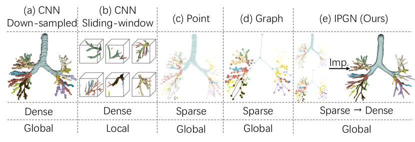
Figure 2: A Comparison of Data Representation for Pulmonary Tree Labeling. The CNN-based methods are either low-resolution (down-sampled) or local (sliding-window). The standard sparse representation like point and graph is global but it is not-trivial to reconstruct high-quality dense volume. Our method that combines point, graph, and implicit functions produces high-quality dense reconstruction efficiently.

2 Related Works

2.1 Pulmonary Anatomy Segmentation

In pulmonary-related studies, image-based understanding of pulmonary anatomies is important as metrics inferred from lung imaging have shown to be related to severity, development and therapeutic outcome of pulmonary diseases[5, 6, 7, 8, 9, 10].

Previously, CNN-based methods have been tailored for comprehension of different pulmonary anatomies, such as pulmonary lobe[19], airway [20]. artery-vein[21, 22] and fissure[23]. Among various pulmonary anatomies, tree-shaped pulmonary structures have drawn a lot of research attention. For pulmonary airway tree, not only is proper segmentation crucial for surgical navigation[7], segmentation-derived attributes like airway counts[6], thickness of wall[11] and morphological changes[8] also have association with lung diseases. For pulmonary vasculature including arteries and veins, quantitative attributes extracted from segmentation are also commonly applied in multiple pulmonary-related medical applications like emboli detection[9] and hypertension[10].

Previous works specifically on pulmonary tree segmentation either apply graph-only modeling or leverage graph-CNN multi-task learning. A Tree-Neural Network[16] leverages handcrafted features on a tailored hyper-graph for pulmonary bronchial tree segmentation to address the inherent problem of overlapping distribution of features. A recent[18] work on airway segmentation proposes graph modeling to incorporate structural context to local CNN feature from each airway branch. Yet, both works merely provide labeling to pulmonary tree branches that are pre-defined at pixel level, and thus are not for semantic segmentation, where defining accurate borders between neighboring branches remains a challenge. Applicable to binary or raw images of pulmonary structures, SG-Net [17] employs CNN features for detecting of landmarks, constructing graphs for CNN-graph multi-task learning.

Although these methods are graph-based, the graph construction procedure varies. While one treats each pre-defined branch as a node[18], disrupting the original spatial structure, another is parameter-based[16], causing the quality of the constructed tree highly dependent on the parameter selection, and finally, the SG-Net[17] established its graph node by learned landmark prediction, whose structural quality can not be ensured. In our setup, the skeleton graphs are based on a thinning algorithm[24], with no modeling or hyper-parameters tuning involved, and all spatial and connection relationships between tree segments are acquired directly from the original dense volume (Fig. 1). Additionally, as CNN methods incur memory footprint that grows in cubical, they are expensive when facing large 3D volumes.

2.2 3D Deep Learning

Deep learning on 3D geometric data is a specialized field that focuses on extending neural networks to handle non-Euclidean domains such as point clouds, graphs (or meshes), and implicit surfaces.

Point-based methods have emerged as a novel approach for 3D geometric modeling. As sparse 3D data, point cloud can be modeled in a variety of ways, such as multi-layer perception[25, 26], convolution [27, 28], graph [29] and transformer [30, 31]. Point-based methods have also been validated in the medical image analysis domain[14, 15].

Since the initial introduction [32], graph learning has become a powerful tool for analyzing graph-structured data, being widely applied to medical images analysis[16, 18, 17] or bioinformatics[33]. Meshes represent a specialized form of graph, typically characterized by a collection of triangular faces to depict the object surfaces, and are extensively employed in the field of graphics. Additionally, they also maintain some applications in the domain of medical imaging [34, 35].

While point-based methods enable computation-efficient modeling on volumetric data, graph learning is lightweight and learns structural context within geometric data. Combining point and graph methods is advantageous in our task. However, extracting surfaces (or dense volumes) from sparse point-based or graph-based prediction is non-trivial, which leads us to introduce implicit surface representation to address this issue.

Deep implicit functions have been successful at modeling 3D shapes [36, 37, 38, 39, 40, 41, 42]. Typically, the implicit function predicts occupancy or signed distance at continuous locations, thus capable of reconstructing 3D shapes at arbitrary resolutions [43]. Moreover, implicit networks could be trained with randomly sampled points, which lowers the computation burden during training. These characteristics suggest that implicit functions have inherent advantages when reconstructing the sparse prediction of pulmonary tree labeling into dense.

3 Problem Formulation

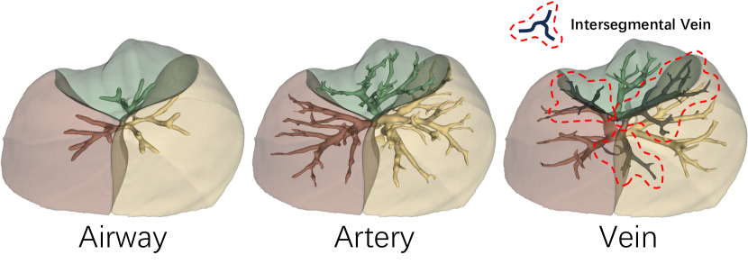
Figure 3: Visualization of Pulmonary Tree and Pulmonary Segment Anatomy. Each pulmonary tree branch corresponds to a pulmonary segment. The intersegmental vein, which lies along the pulmonary segment border, is highlighted in red.

3.1 Pulmonary Tree Labeling

In this study, we address the pulmonary tree labeling problem in 3D CT images. Specifically, given a binary volumetric image of a pulmonary tree, our objective is to provide accurate 19-class segmentation of the pulmonary airway, artery, and vein trees into segmental-level branches and components, demonstrated in Fig. 1 (b). Through this process, each foreground pixel will be assigned to its respective semantic class.

When evaluating the segmentation performance, we consider the presence of intersegmental veins and the potential ambiguity in their class assignment. Intersegmental veins are veins that lie along the border between two neighboring pulmonary segments [44], highlighted in Fig. 3. As pulmonary tree branches are involved in the boundary definition of pulmonary segments[43], intersegmental veins pose an inherent challenge in their class definition. To address this issue, we mask out the intersegmental veins during the evaluation and only focus on segmentation of the pulmonary airway, artery, and veins within each individual segment.

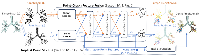
Figure 4: Overview of the proposed Implicit Point-Graph Network (IPGN) for Pulmonary Tree Labeling. The pipeline pre-processes dense volume to graph and point cloud input for feature fusion learning. The Point-Graph Fusion layers enhance point features with graph context, and the Implicit Point Module produces dense prediction efficiently.

3.2 Dataset

3.2.1 Overview

From multiple medical centers, we compile the Pulmonary Tree Labeling (PTL) dataset containing annotated pulmonary tree structures for 800 subjects. For each subject, there are 3 volumetric images containing its pulmonary airway, artery, and vein, illustrated in Fig. 1 (b). In each volume, the annotations consist of 19 classes, where labels 1 to 10 represent branches located in the left lung, labels 11 to 18 represent those in the right lung, and class 19 represents extra-pulmonary structures while 0 is background.

All 3D volumes have shapes $N\times 512\times 512$, where $512\times 512$ represents the CT slice dimension, and $N$ denotes the number of CT slices, ranging from 181 to 798. Z-direction spacings of these scans range from 0.5mm to 1.5mm. Manual annotations are produced by a junior radiologist and verified by a senior radiologist. During the modeling process, the images are converted to binary as input, and the original annotated image is the prediction target. The dataset is randomly split into 70% train, 10% validation, and 20% test samples.

3.2.2 Skeleton Graph

We utilize a software application vesselvio[45], which applies a thinning algorithm[24], to pre-process the volumetric data and derive a skeleton graph in 3D space for each pulmonary structure, illustrated by Fig. 2 (d). The graphs consist of nodes that represent branch bifurcation points and edges that represent anatomical connections. In this manually derived graph dataset, the label for each graph node and edge is recovered from the dense volume. Therefore, the task within this graph dataset involves performing a 19-class classification for both graph nodes and edges.

3.3 Evaluation Metrics

For segmentation performance evaluation, classification accuracy and micro-averaged dice scores are used as metrics. For point-level results on dense volume, the classification accuracy measures the percentage of correctly classified points in the dense volume. The dice score, on the other hand, assesses the overlap between the predicted segment and the ground truth segment, providing a measure of similarity. For graph-level node and edge classification, the same metrics can be applied. The classification accuracy measures the percentage of correctly classified nodes and edges in the pre-processed skeleton graph dataset (Sec. 3.2.2). The dice score can also be used to assess the similarity of the predicted graph structure with the ground truth graph structure.

4 Methodology

Our objective is centered around the anatomical labeling of pulmonary trees. That is to say, given an input of binary volumes of a pulmonary tree—derivable from manual annotations or model predictions—we aim to execute a 19-class semantic segmentation on every non-zero voxel. However, diverging from standard methodologies reliant on CNNs, we down-sample the raw dense volume to a point cloud while concurrently extracting a skeleton graph. Our approach (Sec. 4.1) engages in representation learning individually on the sparse representations of both the point cloud and the skeleton graph, and a fusion module is employed to perform deep integration of point-graph representations (Sec. 4.2). Ultimately, to reconstruct the predictions based on sparse representations back to dense, we introduce implicit functions to facilitate efficient reconstruction (Sec. 4.3).

4.1 Implicit Point-Graph Network Architecture

Given a binary volumetric image of a pulmonary tree (Fig. 4 (a)), a graph (Fig. 4 (b)) is constructed with VesselVio[45] from the original volume and a set of points are randomly sampled from the tree voxels to construct a point cloud (Fig. 4 (c)). While the point cloud is a sparse representation of the volume, the graph represents a skeleton of the pulmonary tree.

We first introduce the general notation rule for both point and graph elements. While the coordinates of $M$ points and $N$ graph nodes are represented as P and G, single point or graph element is expressed as p and g, where $\textbf{P}=\{{\textbf{p}}_{1},\textbf{p}_{2},...,\textbf{p}_{m}\}$, $\textbf{G}=\{\textbf{g}_{1},\textbf{g}_{2},...,\textbf{g}_{n}\}$. The superscript notation $\textbf{p}^{(i)}$ represents an element’s feature at the $i$-th network layer.

At input, the 3-dimensional $\{x,y,z\}$ point coordinates, P $\in$ $\mathbb{R}^{M\times 3}$ and graph nodes, G $\in$ $\mathbb{R}^{N\times 3}$ are utilized as initial feature. We use a point neural network, and a graph neural network as initial feature encoders, from which we extract a 128-dimensional intermediate feature for each point and graph node, expressed as $\textbf{P}^{(0)}$ $\in$ $\mathbb{R}^{M\times 128}$ and $\textbf{G}^{(0)}$ $\in$ $\mathbb{R}^{N\times 128}$.

Subsequently, initial features from both branches $\textbf{P}^{(0)}$ and $\textbf{G}^{(0)}$ are incorporated within one or multiple Point-Graph Fusion layers, which allow for two-way feature integration based on feature propagation[46] and ball-query&grouping[26]. Let the input to a Point-Graph Fusion layer be defined as $\textbf{P}^{(i-1)}$ and $\textbf{G}^{(i-1)}$, the feature out of the fusion layer is $\textbf{P}^{(i)}$ and $\textbf{G}^{(i)}$. The last Point-Graph Fusion layer outputs $\textbf{P}^{(l)}$ and $\textbf{G}^{(l)}$ after $l$ Point-Graph Fusion layers for deep feature fusion. Finally, a lightweight MLP network and a GNN projects the fusion feature to 19-dimensional vectors for graph (Fig. 4 (d)) and point predictions (Fig. 4 (e)).

An Implicit Point Module is further introduced to reconstruct the dense volumes, which consists of a feature propagation process and an MLP network. As features are extracted by the Point-Graph Network, the Implicit Point Module leverages the extracted multi-stage point features for fast dense volume segmentation. Given a query point $\textbf{p}_{q}$ with at arbitrary coordinates, the module locates $p_{q}$’s $k$-nearest point elements from the point cloud: $\{\textbf{p}_{1},\textbf{p}_{2},...,\textbf{p}_{k}\}$, and extracts their multi-stage features $\{\textbf{z}_{1},\textbf{z}_{2},...,\textbf{z}_{k}\}$ from the backbone Network for feature propagation into a multi-stage representation $\textbf{z}_{q}$ of the query point $\textbf{p}_{q}$. After propagating the point feature $\textbf{z}_{q}$, the MLP network $\mathcal{H}$ is utilized to make class predictions. By applying this process to all foreground points, we can efficiently generate a dense volume reconstruction (Fig. 4 (f)).

To avoid naming ambiguity, we refer to the aforementioned complete network as Implicit Point-Graph Network (IPGN), and that sans the implicit part as Point-Graph Network (PGN).

4.2 Point-Graph Feature Fusion

The essence of our point-graph fusion learning approach lies in leveraging coordinate information as a basis for querying neighboring elements in the opposite branch. To achieve feature integration, We adopt ball-query & grouping for point-to-graph feature merging and feature propagation for graph-to-point feature merging.

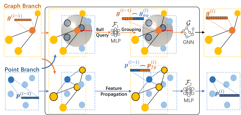
Figure 5: Point-Graph Fusion Layer. The details of the Point-Graph Fusion layer are presented. Here, $\mathcal{F}_{1}$ and $\mathcal{F}_{2}$ are MLP networks while $\mathcal{G}$ represents a graph neural network.

For the ball-query & grouping method in the $i$-th Point-Graph Fusion layer, a graph node $g$ searches for all opposite point elements within a given ball with radius $r$ as $\{\textbf{p}_{1},\textbf{p}_{2},...,\textbf{p}_{b}\}$. Then, an MLP module $\mathcal{F}_{1}:\mathbb{R}^{D}\rightarrow\mathbb{R}^{D}$ independently project the point feature vectors to an updated representation of all queried points, Then, a feature-wise max-pooling layer aggregates all updated point features as point representation of the node g, expressed as:

$$\textbf{g}^{(i)}_{bq}=\max_{j}\left(\mathcal{F}_{1}(\textbf{p}^{(i-1)}_{j})\right)$$ (1)

Subsequently, the ball-queried feature $\textbf{g}^{(i)}_{bq}$ is combined with the current feature $\textbf{g}^{(i-1)}$ before using a graph neural network $\mathcal{G}:\mathbb{R}^{2D}\rightarrow\mathbb{R}^{D_{next}}$ to perform graph convolution for feature fusion, resulting an updated feature representation of the node, $\textbf{g}^{(i)}$ $\in$ $\mathbb{R}^{D_{next}}$, as input to the next Point-Graph Fusion layer.

For feature fusion from graph to point, feature propagation is utilized. In the process, each query point p with feature $\emph{p}^{(i-1)}$ $\in$ $\mathbb{R}^{D}$ at the $i$-th fusion layer locates its $k$-nearest graph nodes $\{\emph{n}_{1},\emph{n}_{2},...,\emph{n}_{k}\}$ in coordinate space. With $k$-nearest neighbors, the query point p acquires summarized graph feature $\textbf{p}^{(i)}_{fp}$ by weighted summation (Eq. 2) of the $k$ node features $\{\textbf{g}^{(i-1)}_{1},\textbf{g}^{(i-1)}_{2},...,\textbf{g}^{(i-1)}_{k}\}$ $\in$ $\mathbb{R}^{D}$, where the weights are based on the normalized reciprocal distances. Let the distance between the query point and $k$ neighbor nodes be $\{\emph{d}_{1},\emph{d}_{2},...,\emph{d}_{k}\}$, the propagation can be expressed as:

$$\textbf{p}^{(i)}_{fp}=\frac{\sum_{j=1}^{k}{\textbf{g}^{(i-1)}_{j}\times\frac{1}{d_{j}}}}{\sum_{l=1}^{k}\frac{1}{d_{l}}}$$ (2)

Then, the aggregated feature for point p, $\textbf{p}^{(i)}_{fp}$ $\in$ $\mathbb{R}^{D}$ is concatenated with the incoming point feature $\textbf{p}^{(i-1)}$ to create $\textbf{p}^{(i)}_{concat}$ $\in$ $\mathbb{R}^{2D}$. Finally, an MLP module $\mathcal{F}_{2}:\mathbb{R}^{2D}\rightarrow\mathbb{R}^{D_{next}}$ projects the concatenated point feature to the input dimension of the next layer as $\textbf{p}^{(i)}$ $\in$ $\mathbb{R}^{D_{next}}$.

4.3 Implicit Dense Volume Reconstruction

To acquire dense volume segmentation results, the naive method is to sample all points from the pulmonary tree and group into multiple non-overlapping point clouds for full inferences. For example, for a point cloud containing $6k$ points, when the total number of foreground points in dense volume is around $180k$, the number of forward passes required to reconstruct the dense would be around $30$. However, repeated inferences is computationally inefficient because the graph input remains identical and the point cloud is globally invariant during the $30$ inferences.

Figure 6: Implicit Point Module. For any query point, the Implicit Point Module consumes multi-stage features from a Point-Graph Network with feature propagation and a neural network to provide a label. $\mathcal{H}$ represents an MLP.

To avoid repetitive computation, we propose the Implicit Point Module in Fig. 6 for efficient and arbitrary point inference, enabling fast dense volume reconstruction in 3-steps. First, for arbitrary point coordinates $\textbf{p}_{q}=(x_{q},y_{q},z_{q})\in\mathbb{R}^{3}$ as input, its $k$ nearest-neighbor points $\{\textbf{p}_{1},\textbf{p}_{2},...,\textbf{p}_{k}\}$ in point cloud (Fig. 6 (a)) are queried. Second, for the $i$-th nearest neighbor point $p_{i}$, its corresponding features in different stages of the network are extracted and concatenated to form a multi-stage feature vector $\textbf{z}_{i}=\{\textbf{p}^{(0)}_{i}\frown\textbf{p}^{(1)}_{i}\frown...\frown\textbf{p}^{(l)}_{i}\}$, where $l$ denotes the number of Point-Graph Fusion layers. A feature propagation (Fig. 6 (b)), similar to Eq. 2, is performed to aggregate $\{\textbf{z}_{1},\textbf{z}_{2},...,\textbf{z}_{k}\}$ into the feature representation $\textbf{z}_{q}$ for the query point. Finally, an MLP network $\mathcal{H}$ projects the feature $\textbf{z}_{q}$ into a 19-dimensional vector for final classification (Fig. 6 (c)). For dense volume segmentation results, simply sample all foreground points and query through the module for prediction.

4.4 Model Details

The IPGN is a customizable pipeline. For ball query in point-to-graph fusion, we set ball radius $r$ = 0.1, and the maximum queried point is 24. For feature propagation in both graph-to-point fusion and the Implicit Point Module, we set $k$=3 for the $k$-nearest neighbor search. During the entire Point-Graph Network backbone, we set the intermediate fusion features to be 128-dimensional.

4.4.1 Training

At the point branch, we experimented with two point models, PointNet++ [26] or Point Transformer [31] as initial feature encoders. For the graph encoder, we apply an 11-layer GAT[47] as the initial feature encoder. Prior to the training of the network, the feature encoders at point and graph branches are independently trained on the corresponding point and graph segmentation tasks and kept frozen.

The Point-Graph Network and the Implicit Point Module are trained simultaneously. First, we perform a forward pass on the Point-Graph Network, generating multi-stage point and graph features as well as predictions for the $M$ input points and $N$ graph elements. Subsequently, another set of $M^{\prime}$ foreground points are randomly sampled, and perform forward inference on the Implicit Point Module for $M^{\prime}$ predictions. After acquiring $M+M^{\prime}$ point and $N$ graph predictions, we apply the Cross-Entropy loss for training.

The two point encoder candidates: PointNet++ and Point Transformer, are both trained for 120 epochs with a learning rate of 0.002 while the GAT graph encoder is trained for 240 epochs with a learning rate of 0.02. The IPGN pipeline is trained for 100 epochs with a learning rate of 0.01 and for every 45 epochs, the learning rates are divided by 2. To improve model robustness, we employ random rotation, shift, and scaling as data augmentation during training.

4.4.2 Inference

Testing on the dense volume input involves a 2-step procedure. First, the input point cloud and graph perform inference and generate multi-stage features through the backbone Point-Graph Network. In the second step, we sample all foreground points on the pulmonary tree structure and feed them to the Implicit Point Module in an iterative manner for predictions. With predictions for all dense volume elements, we simply reconstruct the volume by placing the predicted point labels at the 3D coordinates.

5 Experiments

				Airway						Artery						Vein
	Feature			Point-level		Graph-level				Point-level		Graph-level				Point-level		Graph-level
						Node		Edge				Node		Edge				Node		Edge
Methods	CNN	Point	Graph	Acc	Dice	Acc	Dice	Acc	Dice	Acc	Dice	Acc	Dice	Acc	Dice	Acc	Dice	Acc	Dice	Acc	Dice
Voxel / Point
3D-Unet (down-sampled)[48]	✓			62.9	58.5	-	-	-	-	67.1	61.4	-	-	-	-	63.0	54.0	-	-	-	-
3D-Unet (down-sampled) + KP[17]	✓			63.6	56.9	-	-	-	-	67.2	61.3	-	-	-	-	63.7	55.0	-	-	-	-
3D-Unet (sliding-window)[48]	✓			61.0	39.8	-	-	-	-	51.0	22.5	-	-	-	-	52.6	28.7	-	-	-	-
PointNet[25]		✓		87.4	79.1	-	-	-	-	86.6	80.0	-	-	-	-	79.6	70.8	-	-	-	-
PointNet++[26]		✓		90.1	82.9	-	-	-	-	89.0	82.5	-	-	-	-	82.5	75.7	-	-	-	-
Point Transformer[31]		✓		91.1	87.8	-	-	-	-	90.1	86.5	-	-	-	-	83.4	77.7	-	-	-	-
Graph
GCN[32]			✓	84.0	82.8	87.8	85.5	85.5	83.0	80.2	79.6	83.2	82.1	81.8	80.4	74.6	73.7	74.7	73.5	71.7	70.4
GIN[49]			✓	85.3	84.6	90.5	88.8	87.6	85.6	82.1	81.4	86.0	84.9	84.3	82.8	75.0	74.0	75.8	74.3	72.5	70.9
GraphSage[50]			✓	86.6	86.0	92.8	91.7	89.5	88.0	83.0	82.4	87.8	86.7	85.8	84.5	76.7	75.9	79.9	79.1	76.1	75.0
HyperGraph[16]			✓	86.7	86.0	93.4	93.0	89.2	88.8	82.9	82.2	89.3	89.0	86.3	85.7	76.4	75.7	79.6	79.4	76.1	75.8
HyperGraph + Handcrafted Features[16]			✓	86.4	85.8	93.0	92.8	88.9	88.7	82.5	81.8	89.0	88.6	86.1	85.2	76.3	75.7	79.6	79.5	75.8	75.4
GAT[47]			✓	86.9	86.3	94.1	92.7	90.8	89.1	84.0	83.4	89.6	88.7	87.6	86.3	76.7	76.0	80.3	79.0	76.7	75.3
GAT [47] + Handcrafted Features [16]			✓	86.9	86.3	94.0	92.5	90.7	88.8	84.1	83.7	89.4	88.4	87.4	86.2	77.1	76.1	79.5	78.1	75.6	74.1
Point + Graph
GAT [47] (PointNet++ Features)[26]		✓	✓	87.2	86.7	94.4	94.6	91.7	91.8	84.5	83.8	91.8	90.5	89.1	88.6	77.6	76.3	81.8	80.4	78.3	77.0
PGN (PointNet++[26])		✓	✓	91.0	87.7	95.2	95.1	92.3	92.3	89.9	86.8	92.9	92.9	90.0	89.9	83.8	77.4	82.9	82.8	79.6	79.4
IPGN (PointNet++[26])		✓	✓	91.0	87.5	95.2	95.1	92.3	92.3	89.9	86.6	92.9	92.9	90.0	89.9	83.6	77.5	82.9	82.8	79.6	79.4
PGN (Point Transformer[31])		✓	✓	91.6	88.4	95.3	95.0	92.6	92.7	90.7	87.2	93.0	92.6	90.2	89.9	83.8	78.6	82.5	82.3	78.7	78.8
IPGN (Point Transformer[31])		✓	✓	91.5	88.5	95.3	95.0	92.6	92.7	90.7	87.2	93.0	92.6	90.2	89.9	83.7	78.3	82.5	82.3	78.7	78.8

Table 1: Model Performance at Graph-Level and Point-Level on the PTL dataset. This table contains performance metrics results at point-level and graph-level. Different baseline methods using different feature contexts are presented to compare against the proposed methods on the Pulmonary Tree Labeling dataset. PGN: Point-Graph Network without implicit functions. IPGN: Implicit Point Graph Network.

5.1 Experiment Setting

By default, all experiments use dense volume as initial input. While CNN is natural for manipulating dense volume, we pre-process the dense volume to point clouds and skeleton graphs for point and graph experiments. We present the experiment metrics at the point-level and graph-level. The performance at graph-level represents how structural components and connections within a graph are recognized. Moreover, point-level dense volume performance evaluation can be achieved using CNN methods, point-based methods with repeated inferences and graph-based models after post-processing (section 5.1.3). Therefore, the evaluations in point-level across convolution, point, and graph methods are consistent and fair.

5.1.1 CNNs

In CNN experiments, given a 3D input, the task involves providing semantic segmentation prediction for the pulmonary tree in the image and all CNN methods apply a combination of dice loss and the cross-entropy loss for training. During testing, the image background is excluded from the metric computation.

Among the CNN experiments, we employ 3D-unet[48] as the basic setup. Based on the 3D-Unet, we also implement a multi-task key-point regression method[17], abbreviated as ”3D-Unet + KP”. More specifically, an additional regression prediction head predicts a heatmap representing how likely is the location of a graph node as a key-point. In these two CNN-based experiments, data are down-sampled to $96\times 96\times 96$ due to limited GPU memory during training and validation. During testing, the input is down-sampled for inference and re-scaled to the original dimension $N\times 512\times 512$ for evaluation.

To address the issue of high memory usage and information loss by compromised resolution, we apply a sliding window approach in another CNN experiment, in which local 3D patches with dimension $96\times 96\times 96$ from the original image are used for training and validation purposes. During testing, the predictions obtained from the sliding-window technique were assembled back onto the original image for evaluation.

5.1.2 Point Clouds

Point-based experiments involve treating a set of tubular voxels of a pulmonary tree as a point cloud for sparse representation for modeling. At the output, point-based model provides per-point classification prediction.

During training and validation of the experiments, we randomly sampled 6000 foreground elements as point cloud input. During testing, all foreground points are sampled, randomly permuted, and grouped into multiple point clouds. Then each point cloud containing 6000 points is iteratively fed into the model for evaluation. Consequently, the inference processes provide a prediction for all foreground elements as dense volume results. In terms of baselines, PointNet[25], PointNet++[26] and Point Transformer[31] are tested.

5.1.3 Graphs

Graph experiments utilize the skeleton graph generated from dense volume by software[45] as graph structure, and evaluate networks’ ability to recognize key-point and structural connections within the skeleton tree, respectively represented by per-node and per-edge performance.

In graph experiments, we leverage multiple graph neural networks (GNN) such as GAT[47], GraphSage[50], and graph network with pre-trained point-based features as input. We ensure fair comparisons across all GNNs by using 14 respective layers. After acquiring node features, features from the source node and destination node are interpolated by averaging for edge features before an MLP network projects all features to 19-dimension for final predictions.

Furthermore, we implement a post-processing technique to dilate graph-based prediction to dense volume prediction. Specifically, given any voxel, the algorithm searches for the label of the nearest graph element as its own label. Therefore, all graph baselines also provide point-level prediction metrics.

5.1.4 Ours

As discussed in depth in section 4, we perform experiments combining point learning with graph learning. For the proposed Point-Graph network, the input and output setups for the point branch and graph branch are identical to those of point experiments and graph experiments. To speed up dense reconstruction, we incorporate the Implicit Point Module for point-based prediction, evaluated at point-level.

5.2 Model Performance Comparison

In this section, we perform a comparative analysis based on Table 1. The statistics presented in this section are the average performance over the 3 pulmonary structures.

At graph-level evaluation, among GNN methods with graph-only context, GAT[47] model, with minimal tuning, outperforms most baselines with considerable margin, displaying the advantage of attention mechanism in pulmonary tree setting. In addition to graph modeling with 3D coordinate features, the performance of the GAT[47] model, and a hypergraph[16] model with handcrafted features[16] are presented. Compared to applying coordinate features as input, GAT with handcrafted features suffers from a slight drop of 0.4% in accuracy. On the other hand, applying handcrafted features to the hypergraph[51] model also translates to a performance drop. These results suggest that in graph settings, tailor-designed features don’t provide more valuable information than 3D coordinates. Further insights are provided in section 5.5.1.

For graph performance in settings with both graph and point context, GAT (PointNet++ feature) has the lowest performance among all. Nevertheless, it still outperforms any other graph-context-only baseline by a margin of around 1.4% in accuracy at minimum. Such a gap in performance indicates that the integration of point-context into graph learning is beneficial. For the proposed Point-Graph Network and IPGN, their performances beat all baselines in both metrics, displaying superiority in point-graph fusion learning.

At point-level, CNN methods achieve the worst performance. Two 3D-Unet[48, 17] methods based on down-sampled input yield unsatisfying metrics, indicating that training CNN methods on reduced resolution leads to inferior modeling. As an attempt to train on the original resolution without memory restriction, the 3D-Unet[48] experiment with sliding-window strategy reports the poorest performances at both accuracy and dice, likely due to lack of global context.

Among point-based methods, the Point Transformer[31] achieves the overall best performances. In terms of graph-based methods, their point-level results generally report lower accuracy, while offering relatively high dice scores compared to point baselines despite the lack of local shape context: The highest dice score from graph methods is only 1.7% behind that of Point Transformer. In our view, such dice quality based on graph can be attributed to the accurate prediction of graph nodes, which is equivalent to border prediction as nodes represent bifurcation points in a tree. Additionally, in CNN, point-based, and the point-graph fusion methods, accuracy is generally higher than dice score. We believe that because the extra-pulmonary structure (Fig. 1, colored in light blue) possesses a large volume and has a distinct location, it could be easily recognized, boosting the accuracy over the dice score.

For settings with point and graph context, the proposed Point-Graph Network and IPGN based on pre-trained PointNet++[26] feature reports similar performance as Point Transformer[31], showing that tree-topology context provides a similar benefit as the long-range dependency information from Point Transformer. Point-Graph Network and IPGN based on Point Transformer achieve SOTA results among all settings.

5.3 Dense Volume Reconstruction

Methods	Model	Airway			Artery			Vein
		Time (s)	Acc (%)	Dice (%)	Time (s)	Acc (%)	Dice (%)	Time (s)	Acc (%)	Dice (%)
Voxel	3D-Unet[48] (downsampled)	8.16	62.9	58.5	8.02	67.1	61.4	7.46	63.0	54.0
Voxel	3D-Unet[48] (sliding-window)	9.43	61.0	39.8	11.88	51.0	22.5	12.44	52.6	28.7
Point	PointNet++[26]	4.51	90.1	82.9	9.17s	89.0	82.5	9.65	82.5	75.7
Point	Point Transformer[31]	10.97	91.1	87.8	21.94	90.1	86.5	23.25	83.4	77.7
Graph	GAT[47]	1.15	86.9	86.3	2.05	84.0	83.4	2.24	76.7	76.0
Point + Graph	PGN (PointNet++[26])	5.65	91.0	87.7	12.40	89.9	86.8	13.16	83.8	77.6
Point + Graph	IPGN (PointNet++[26])	1.30	91.0	87.5	1.49	89.9	86.6	1.57	83.6	77.5
Point + Graph	PGN (Point Transformer[31])	12.10	91.6	88.4	24.28	90.7	87.2	25.81	83.8	78.6
Point + Graph	IPGN (Point Transformer[31])	2.32	91.5	88.5	2.29	90.7	87.2	2.39	83.7	78.3

Table 2: Inference Speed and Segmentation Metrics. This table compares the dense volume segmentation test time and quality across graph-based, point-based, and point-graph fusion methods. The test times are measured in seconds while accuracy and dice score present segmentation quality.

In this subsection, we focus on the Implicit Point Module (Fig. 6), which aims to enhance the efficiency of labeled dense volume reconstruction (Fig. 4 (f)). As discussed previously in Sec. 1, the integration of the implicit module is necessary as high-performing point models like Point Transformer[31] could still be computationally expensive at test time: with repeated inferences for dense prediction, its computation cost grows in cubicle, similar to CNN. Experiments are completed to compare the efficiency using the Point Implicit module against using the Point-Graph Network as well as various baseline methods. The reconstruction efficiency is represented as the average run-time in seconds, for dense volume prediction across the Pulmonary Tree Labeling test set.

Regarding volume reconstruction efficiency, the test time of convolution methods, graph-based method, point-based method, and our methods were measured. For all setups, we evaluate and present the inference time and quality for dense volume segmentation in Table 2. Apart from model inference costs, test time is composed of various operations in different setups. For CNN with down-sampled input, test time includes down-sampling and up-sampling operations. For graph baselines, time measurement takes post-processing into account. Finally, test time for IPGN includes a forward pass on the Point-Graph Network and the subsequent Implicit Point Module inference on all remaining points.

The results demonstrated the superiority of the IPGN in dense volume reconstruction. Qualitatively, the Point-Graph Network and IPGN achieve nearly identical performance. In terms of efficiency, IPGN only requires $1.5$ seconds on average with PointNet++[26] as point encoder and $2.3$ seconds with Point Transformer[31]. Although the graph-based method records a similar time cost, it fails to generate quality results. Further, all other methods are relatively inefficient. Therefore, the proposed IPGN pipeline is the all-around optimal solution for dense volume segmentation for pulmonary structures.

These findings highlight the practical utility of the proposed module, as it allows for fast and efficient point inference without compromising quality. The Implicit Point Module serves as a valuable contribution in overcoming the computational challenges associated with analyzing the pulmonary tree, enabling rapid decision-making in clinical settings.

5.4 Qualitative Analysis with Visualization

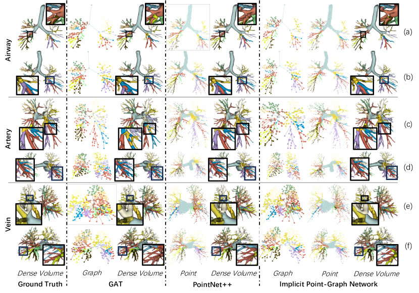
Figure 7: Visualization of Segmentation Results. This figure displays segmentation results using GAT[47] (graph-only context), PointNet++[26] (point-only context) and IPGN (with GAT and PointNet++ backbones) methods along with the ground truth. For each method class, the corresponding predictions in their initial form prior to dense volume prediction are also presented.

In the qualitative analysis section, we employ 2 concrete cases each from the airway, artery, and vein tree to demonstrate the efficacy of our method. Fig. 7 (a-f) showcases the results of full pulmonary tree segmentation using graph-only method, point-only method, and the Implicit Graph-Point Network, against the ground truth image.

The graph-based predictions from Fig. 7 (b-d) reveal instances of incorrect graph predictions leading to anomalous outcomes, where multiple class labels appear in the same branch, thereby inducing inconsistent branch predictions. For point-based method, due to its sparse representation in individual forward passes, point predictions often lose details and disrupt the borders between branches (Fig. 7 (a,c,e)), resulting in volumes that lack smoothness and quality.

Conversely, the proposed IPGN offers various advantages. Firstly, our method accurately classifies distal branches, illustrated by dense volume prediction in Fig. 7 (d,f). Additionally, our method effectively defines clear and uninterrupted borders between the child branches at bifurcation points. This is especially valuable when a parent node branches into multiple child branches belonging to different classes, as demonstrated in Fig. 7 (b,e). By integrating graph and point context into the modeling process, our method enhances the segmentation capabilities at bifurcation points and distal branches, ultimately producing smoother and more uniform branch predictions.

5.5 Ablation Experiments

5.5.1 Feature Input Selection

In this section, we examine the effect of different input features for the skeleton graph node. The candidates are 3D coordinates feature and handcrafted feature. As coordinate feature is simply the $\{x,y,z\}$ coordinates, handcrafted feature follows the feature design from TNN[16], containing structural, positional, and morphological features.

We perform experiments on a GAT[47] and a 5-layer MLP network to evaluate the impact of coordinate features and handcrafted features, reported in Table 3. Based on the MLP experiment, handcrafted feature achieves 81.4% node accuracy on average while raw coordinate only reports 74.4%. Conversely, in the experiment with GAT[47], applying the coordinate feature achieves overall best performances, reaching 88.17% while the handcrafted feature trails behind.

The results indicate that the handcrafted feature provides more information and produces better performance in an MLP setting, where the neural network simply learns a non-linear projection without any global or tree topology context. Once the connections between graph nodes are established through edge in graph modeling, the handcrafted feature completely loses its advantages over the raw coordinate feature, which implies that the handcrafted feature could be learned during graph learning and the learned graph-based feature is more beneficial to graph segmentation quality.

Method	Features		Airway		Artery		Vein
	Handcrafted	Raw Coord	Node Acc	Edge Acc	Node Acc	Edge Acc	Node Acc	Edge Acc
MLP	✓		84.6	-	81.3	-	78.4	-
		✓	72.4	-	76.1	-	74.6	-
	✓	✓	84.4	-	81.2	-	78.5	-
GAT[47]	✓		93.3	90.1	89.4	76.5	79.8	75.9
		✓	94.0	90.4	90.0	88.2	80.5	77.2
	✓	✓	93.6	90.6	89.5	87.5	79.8	76.1

Table 3: Impact of Feature Input. This table shows the experiment results using a GAT[47] model and an MLP network for modeling on different feature inputs.

5.5.2 Input Selection For Implicit Point Module

In this section, we present the results of an ablation study where we explore the impact of multi-stage features using different layers of the intermediate feature vector as input to the implicit module.

In the experiment, we initially utilized the feature output of the final Point-Graph Fusion layer as the sole input to the implicit module. Motivated by the design of DenseNet[52], we experimented with adding feature outputs from shallower intermediate blocks, forming multi-stage features, and report the performance with each feature addition until the initial point feature. Table 4 demonstrates that combining multi-stage features, along with the initial point (PointNet++[26]) feature, enhances the predictive capabilities of our model, contributing to better performance. Finally, the best-performing configuration we observed involved using all available features, yielding results on par with the full modeling approach.

	$\textbf{P}^{(3)}$	$\textbf{P}^{(2)}\frown\textbf{P}^{(3)}$	$\textbf{P}^{(1)}\frown\textbf{P}^{(2)}\frown\textbf{P}^{(3)}$	$\textbf{P}^{(0)}\frown\textbf{P}^{(1)}\frown\textbf{P}^{(2)}\frown\textbf{P}^{(3)}$
Airway	90.7	90.8	90.9	91.0
Artery	89.6	89.7	89.9	89.9
Vein	82.9	83.3	83.6	83.6

Table 4: Multi-stage Point Feature Input for Implicit Point Module. This table presents the results using different combinations of concatenated multi-stage features from the backbone network as input to the Point Implicit Module.

6 Extended Application:
Reconstruction of Pulmonary Segments

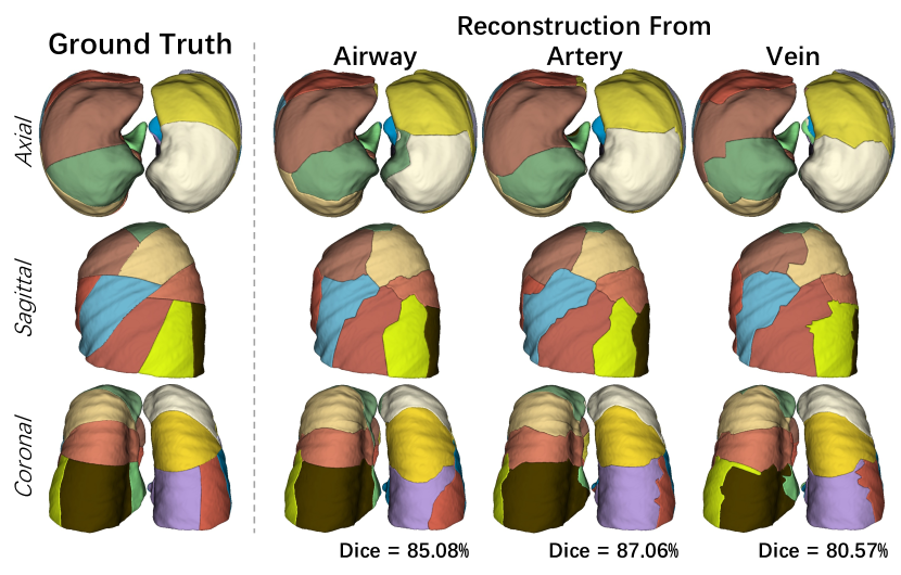
Figure 8: Pulmonary Segments Visualization. The pulmonary segments reconstruction based on the airway, artery, and vein trees is presented against ground truth in multiple views.

The Implicit Point Module plays a vital role in defining implicit surfaces between different classes within the pulmonary tree, allowing for efficient dense reconstruction of the pulmonary tree. As the module utilizes the point-graph feature field for labeling, the input coordinates are not constrained to the tubular voxel/point. Consequently, any point within the pulmonary lobe can be assigned a class label.

Pulmonary segments are subdivisions within the pulmonary lobes and their boundaries are determined based on the 18 branches of the pulmonary trees of our interest[43]. By utilizing the extracted point-graph feature field from the airway, artery, or vein tree, our module can accurately infer information for all points within the lobe. This enables us to achieve a natural semantic reconstruction of the pulmonary segments, depicted in Fig. 8.

Compared to the ground truth, the tree-segmentation-induced pulmonary segments reconstruction achieves 80.13%, 82.15% and 76.20% prediction accuracy and 79.89%, 81.85% and 76.16% micro-average dice scores, respectively for pulmonary airway, artery, and vein. Future works can potentially produce better pulmonary segment reconstruction by integrating features from the three pulmonary trees or leveraging the explicit pulmonary lobe boundaries as additional guidelines.

7 Conclusion

In conclusion, we take an experimentally comprehensive deep-dive into pulmonary tree segmentation based on the compiled PTL dataset. A novel architecture Implicit Point-Graph Network (IPGN) is presented for accurate and efficient pulmonary tree segmentation. Our method leverages a dual-branch point-graph fusion model to effectively capture the complex branching structure of the respiratory system. Extensive experiment results demonstrate that by implicit modeling on point-graph features, the proposed model achieves state-of-the-art segmentation quality with minimum computation cost for practical dense volume reconstruction. The advancements made in this study could potentially enhance the diagnosis, management, and treatment of pulmonary diseases, ultimately improving patient outcomes in this critical area of healthcare.

References

- [1] M. Decramer, S. I. Rennard et al., “Copd as a lung disease with systemic consequences – clinical impact, mechanisms, and potential for early intervention,” COPD: Journal of Chronic Obstructive Pulmonary Disease, vol. 5, pp. 235 – 256, 2008.
- [2] P. M. Marcus, E. J. Bergstralh, R. M. Fagerstrom, D. E. Williams, R. S. Fontana, W. R. Taylor, and P. C. Prorok, “Lung cancer mortality in the mayo lung project: impact of extended follow-up.” Journal of the National Cancer Institute, vol. 92 16, pp. 1308–16, 2000.
- [3] C. Nunes, A. M. Pereira, and M. Morais‐Almeida, “Asthma costs and social impact,” Asthma research and practice, vol. 3, 2017.
- [4] S. Quaderi and J. R. Hurst, “The unmet global burden of copd,” Global Health, Epidemiology and Genomics, vol. 3, 2018.
- [5] J.-P. Charbonnier, E. Pompe et al., “Airway wall thickening on ct: Relation to smoking status and severity of copd.” Respiratory medicine, vol. 146, pp. 36–41, 2019.
- [6] M. Kirby, N. Tanabe et al., “Computed tomography total airway count is associated with number of micro-ct terminal bronchioles.” American journal of respiratory and critical care medicine, 2019.
- [7] Y. Qin, M. Chen, H. Zheng, Y. Gu, M. Shen, J. Yang, X. Huang, Y. M. Zhu, and G.-Z. Yang, “Airwaynet: A voxel-connectivity aware approach for accurate airway segmentation using convolutional neural networks,” ArXiv, vol. abs/1907.06852, 2019.
- [8] R. J. Shaw, R. Djukanović et al., “The role of small airways in lung disease.” Respiratory medicine, vol. 96 2, pp. 67–80, 2002.
- [9] P. A. Loud, D. S. Katz et al., “Deep venous thrombosis with suspected pulmonary embolism: Detection with combined ct venography and pulmonary angiography,” Radiology, vol. 219, no. 2, pp. 498–502, 2001, pMID: 11323478.
- [10] Y. Shen, C. Wan et al., “Ct-base pulmonary artery measurement in the detection of pulmonary hypertension: a meta-analysis and systematic review.” Medicine, vol. 93 27, p. e256, 2014.
- [11] B. M. Smith, E. A. Hoffman et al., “Comparison of spatially matched airways reveals thinner airway walls in copd. the multi-ethnic study of atherosclerosis (mesa) copd study and the subpopulations and intermediate outcomes in copd study (spiromics),” Thorax, vol. 69, no. 11, pp. 987–996, 2014.
- [12] Z. Zhou, M. M. R. Siddiquee et al., “Unet++: A nested u-net architecture for medical image segmentation,” DLMIA MICCAI Workshop, vol. 11045, pp. 3–11, 2018.
- [13] Z. Zhou, M. M. R. Siddiquee, N. Tajbakhsh, and J. Liang, “Unet++: Redesigning skip connections to exploit multiscale features in image segmentation,” IEEE Transactions on Medical Imaging, vol. 39, no. 6, pp. 1856–1867, 2019.
- [14] J. Yang, S. Gu et al., “RibSeg dataset and strong point cloud baselines for rib segmentation from CT scans,” in Conference on Medical Image Computing and Computer Assisted Intervention. Springer International Publishing, 2021, pp. 611–621.
- [15] L. Jin, S. Gu, D. Wei, J. K. Adhinarta, K. Kuang, Y. J. Zhang, H. Pfister, B. Ni, J. Yang, and M. Li, “Ribseg v2: A large-scale benchmark for rib labeling and anatomical centerline extraction,” IEEE Transactions on Medical Imaging, 2023.
- [16] W. Yu, H. Zheng et al., “Tnn: Tree neural network for airway anatomical labeling,” IEEE Transactions on Medical Imaging, vol. 42, no. 1, pp. 103–118, 2023.
- [17] Z. Tan, J. Feng, and J. Zhou, “Sgnet: Structure-aware graph-based network for airway semantic segmentation,” in Conference on Medical Image Computing and Computer Assisted Intervention. Cham: Springer International Publishing, 2021, pp. 153–163.
- [18] W. Xie, C. Jacobs, J.-P. Charbonnier, and B. van Ginneken, “Structure and position-aware graph neural network for airway labeling,” arXiv Preprint, vol. abs/2201.04532, 2022.
- [19] S. E. Gerard and J. M. Reinhardt, “Pulmonary lobe segmentation using a sequence of convolutional neural networks for marginal learning,” International Symposium on Biomedical Imaging, pp. 1207–1211, 2019.
- [20] M. Zhang, Y. Wu et al., “Multi-site, multi-domain airway tree modeling,” Medical Image Analysis, p. 102957, 2023.
- [21] P. Nardelli, D. Jimenez-Carretero et al., “Pulmonary artery–vein classification in ct images using deep learning,” IEEE Transactions on Medical Imaging, vol. 37, pp. 2428–2440, 2018.
- [22] Y. Qin, H. Zheng et al., “Learning tubule-sensitive cnns for pulmonary airway and artery-vein segmentation in ct,” IEEE Transactions on Medical Imaging, vol. 40, pp. 1603–1617, 2020.
- [23] S. E. Gerard, T. J. Patton et al., “Fissurenet: A deep learning approach for pulmonary fissure detection in ct images,” IEEE Transactions on Medical Imaging, vol. 38, pp. 156–166, 2019.
- [24] T. Lee, R. Kashyap, and C. Chu, “Building skeleton models via 3-d medial surface axis thinning algorithms,” CVGIP: Graphical Models and Image Processing, vol. 56, no. 6, pp. 462–478, 1994.
- [25] C. Qi, H. Su, K. Mo, and L. J. Guibas, “Pointnet: Deep learning on point sets for 3d classification and segmentation,” Conference on Computer Vision and Pattern Recognition, pp. 77–85, 2016.
- [26] C. Qi, L. Yi, H. Su, and L. J. Guibas, “Pointnet++: Deep hierarchical feature learning on point sets in a metric space,” in Advances in Neural Information Processing Systems, 2017.
- [27] Y. Li, R. Bu et al., “Pointcnn: Convolution on x-transformed points,” Conference on Computer Vision and Pattern Recognition, 2018.
- [28] Z. Liu, H. Tang, Y. Lin, and S. Han, “Point-voxel cnn for efficient 3d deep learning,” ArXiv, vol. abs/1907.03739, 2019.
- [29] Z.-H. Lin, S. Y. Huang, and Y. Wang, “Convolution in the cloud: Learning deformable kernels in 3d graph convolution networks for point cloud analysis,” Conference on Computer Vision and Pattern Recognition, pp. 1797–1806, 2020.
- [30] J. Yang, Q. Zhang et al., “Modeling point clouds with self-attention and gumbel subset sampling,” in Conference on Computer Vision and Pattern Recognition, 2019, pp. 3323–3332.
- [31] H. Zhao, L. Jiang, J. Jia, P. H. Torr, and V. Koltun, “Point transformer,” in International Conference on Computer Vision, 2021, pp. 16 259–16 268.
- [32] T. Kipf and M. Welling, “Semi-supervised classification with graph convolutional networks,” arXiv Preprint, vol. abs/1609.02907, 2016.
- [33] J. M. Jumper, R. Evans et al., “Highly accurate protein structure prediction with alphafold,” Nature, vol. 596, pp. 583 – 589, 2021.
- [34] U. Wickramasinghe, E. Remelli, G. Knott, and P. Fua, “Voxel2mesh: 3d mesh model generation from volumetric data,” in Conference on Medical Image Computing and Computer Assisted Intervention. Springer, 2020, pp. 299–308.
- [35] U. Wickramasinghe, P. Jensen, M. Shah, J. Yang, and P. Fua, “Weakly supervised volumetric image segmentation with deformed templates,” in Conference on Medical Image Computing and Computer Assisted Intervention. Springer, 2022, pp. 422–432.
- [36] Z. Chen and H. Zhang, “Learning implicit fields for generative shape modeling,” Conference on Computer Vision and Pattern Recognition, pp. 5932–5941, 2018.
- [37] J. Chibane, T. Alldieck, and G. Pons-Moll, “Implicit functions in feature space for 3d shape reconstruction and completion,” Conference on Computer Vision and Pattern Recognition, pp. 6968–6979, 2020.
- [38] X. Huang, J. Yang et al., “Representation-agnostic shape fields,” in International Conference on Learning Representations, 2022.
- [39] L. M. Mescheder, M. Oechsle et al., “Occupancy networks: Learning 3d reconstruction in function space,” Conference on Computer Vision and Pattern Recognition, pp. 4455–4465, 2018.
- [40] J. J. Park, P. R. Florence et al., “Deepsdf: Learning continuous signed distance functions for shape representation,” Conference on Computer Vision and Pattern Recognition, pp. 165–174, 2019.
- [41] S. Peng, M. Niemeyer et al., “Convolutional occupancy networks,” arXiv Preprint, vol. abs/2003.04618, 2020.
- [42] J. Yang, U. Wickramasinghe et al., “Implicitatlas: learning deformable shape templates in medical imaging,” in Conference on Computer Vision and Pattern Recognition, 2022, pp. 15 861–15 871.
- [43] K. Kuang, L. Zhang et al., “What makes for automatic reconstruction of pulmonary segments,” arXiv Preprint, vol. abs/2207.03078, 2022.
- [44] H. Oizumi, H. Kato et al., “Techniques to define segmental anatomy during segmentectomy.” Annals of cardiothoracic surgery, vol. 3 2, pp. 170–5, 2014.
- [45] J. R. Bumgarner and R. J. Nelson, “Open-source analysis and visualization of segmented vasculature datasets with vesselvio,” Cell Reports Methods, vol. 2, no. 4, p. 100189, 2022.
- [46] E. Rossi, H. Kenlay et al., “On the unreasonable effectiveness of feature propagation in learning on graphs with missing node features,” ArXiv, vol. abs/2111.12128, 2021.
- [47] P. Velickovic, G. Cucurull et al., “Graph attention networks,” arXiv Preprint, vol. abs/1710.10903, 2017.
- [48] Ö. Çiçek, A. Abdulkadir et al., “3d u-net: Learning dense volumetric segmentation from sparse annotation,” in Conference on Medical Image Computing and Computer Assisted Intervention, 2016.
- [49] K. Xu, W. Hu, J. Leskovec, and S. Jegelka, “How powerful are graph neural networks?” arXiv Preprint, vol. abs/1810.00826, 2018.
- [50] W. L. Hamilton, Z. Ying, and J. Leskovec, “Inductive representation learning on large graphs,” in Advances in Neural Information Processing Systems, 2017.
- [51] Y. Feng, H. You et al., “Hypergraph neural networks,” in Proceedings of the AAAI conference on artificial intelligence, vol. 33, no. 01, 2019, pp. 3558–3565.
- [52] G. Huang, Z. Liu, and K. Q. Weinberger, “Densely connected convolutional networks,” Conference on Computer Vision and Pattern Recognition, pp. 2261–2269, 2016.