Evanescent Electron Wave Spin

Abstract

Our study shows that an evanescent electron wave exists outside both finite and infinite quantum wells, by solving exact solutions of the Dirac equation in a cylindrical quantum well and maintaining wavefunction continuity at the boundary. Furthermore, we demonstrate that the evanescent wave spins concurrently with the wave inside the quantum well, by deriving analytical expressions of the current density in the whole region. Our findings suggest that it is possible to probe or eavesdrop on quantum spin information through the evanescent wave spin without destroying the entire spin state. The wave spin picture interprets spin as a global and deterministic property of the electron wave that includes both the evanescent and confined wavefunctions. This suggests that a quantum process or device based on the manipulation and probing of the electron wave spin is deterministic in nature rather than probabilistic.

I Electron wave spin

The electron spin has attracted significant attention especially in recent years due to its potential applications in information sciences and technologies, such as quantum computing [1],[2] and spintronics [3]. If future computers rely on the precise manipulation of the electron spin, it is crucial to develop a deeper understanding of this property beyond a simplistic interpretation as a superluminal spinning particle.

In recent works [4],[5], it has been argued that the electron spin is a wave property that can be fully described by current densities calculated using the Dirac theorem. The authors demonstrate the existence of a stable circulating current density for an electron confined in an infinite quantum well, which exhibits a multi-vortex topology at excited states. The electron wave spin exhibits geometric and topological characteristics when it interacts with an electromagnetic field, leading to various effects, including fractional spin and modified Zeeman splitting.

It is noted that the electron wave spin was investigated previously in the infinite quantum well, where the wave function outside the well is typically assumed to be zero [6]. Although this model is widely used that has helped gain much insight into many quantum effects inside the quantum well, it assumes the wavefunction outside the well to be exactly zero, which causes a problem in maintaining continuity for both the wavefunction and its derivative at the boundary in both the Schrödinger and Dirac theorems [7]. In reality, all potentials are finite, and therefore, there exists a non-negligible wavefunction outside the well, even when the eigenenergy of the electron is below a finite or an infinite quantum well potential. The wavefunction outside the well shall decay rapidly, thus is evanescent in analogy to the evanescent waves observed in optics.

An intriguing question arises as to whether the evanescent electron wave also spins. An intuitive answer to this question suggests that an evanescent wave shall also spin due to the continuation of wavefunctions and the prevailing algebraic structure of the Dirac equation. The existence of an evanescent wave spin shall raise intriguing possibilities for probing the spin from outside the well without collapsing the spin inside, analogous to the evanescent optical wave sensing [8], [9], [10].

In this paper, we plan to demonstrate the evanescent wave spin by solving the Dirac equation in a quantum well rigorously and obtaining analytical expressions for the wavefunctions and current densities both inside and outside the quantum well. We will demonstrate that the evanescent wave diminishes at high potentials but remains within the skin depth region even for the infinite quantum well due to the wavefunction continuity at the boundary. Finally, we intend to discuss the implications of these findings on quantum detection and quantum information technologies.

II Dirac electron in a finite cylindrical quantum well

We will derive exact solutions of the Dirac equation in a finite cylindrical quantum well and obtain analytical expressions for the current density. The eigenenergy values will be solved numerically through the boundary condition equations.

The Dirac equation in the cylindrical coordinate is

$$\frac{1}{c}\frac{\partial}{\partial t}\psi(\pmb{r},t)=\{-\pmb{\alpha}\cdot\pmb{\nabla}-i\frac{mc^{2}}{\hbar c}\gamma^{0}-i\frac{1}{\hbar c}U(\pmb{r})\}\psi(\pmb{r},t),$$ (1)

where $(\rho,\phi,z)$ represent polar, azimuthal angle and z coordinate, respectively. The operator

$$\pmb{\alpha}\cdot\pmb{\nabla}=\alpha_{\rho}\frac{\partial}{\partial\rho}+\alpha_{\phi}\frac{1}{\rho}\frac{\partial}{\partial\phi}+\alpha_{z}\frac{\partial}{\partial z}$$ (2)

contains $\alpha-$matrix in cylindrical coordinate

$$\alpha_{\rho} = \left(\begin{array}[]{cccc}0&0&0&e^{-i\phi}\\ 0&0&e^{i\phi}&0\\ 0&e^{-i\phi}&0&0\\ e^{i\phi}&0&0&0\\ \end{array}\right);$$ (7)

$$\alpha_{\phi} = \left(\begin{array}[]{cccc}0&0&0&-ie^{-i\phi}\\ 0&0&ie^{i\phi}&0\\ 0&-ie^{-i\phi}&0&0\\ ie^{i\phi}&0&0&0\\ \end{array}\right);$$ (12)

$$\alpha_{z} = \left(\begin{array}[]{cccc}0&0&1&0\\ 0&0&0&-1\\ 1&0&0&0\\ 0&-1&0&0\\ \end{array}\right),$$ (17)

with the following properties

$$\sigma_{\rho}^{2}=\sigma_{\phi}^{2}=\sigma_{z}^{2}=1,$$

$$\sigma_{\rho}\sigma_{\phi}=i\alpha_{z},$$

$$\sigma_{\rho}\sigma_{\phi}+\sigma_{\phi}\sigma_{\rho}=0.$$

We now let the potential

$$U(\pmb{r})=U(\rho)=\Bigl{\{}\begin{array}[]{cc}0,&\rho<R\\ U,&\rho>R\\ \end{array}$$ (19)

represent a finite cylindrical quantum well of potential $U$ and radius $R$. The wavefunction in the quantum well can be expressed by the separation of variables

$$\psi(\pmb{r},t)=e^{-i\mathcal{E}t/\hbar}e^{iP_{z}z/\hbar}\tilde{\psi}(\phi,\rho),$$ (20)

where the momentum along z-direction is set $P_{z}=0$ for our discussion and $\mathcal{E}$ is the eigenenergy to be determined by the boundary conditions.

Plugging Eq. 20 into Eq. 1 to obtain the equation

$$\{-i\frac{\mathcal{E}}{\hbar c}+\alpha_{\rho}\frac{\partial}{\partial\rho}+\alpha_{\phi}\frac{1}{\rho}\frac{\partial}{\partial\phi}+i\frac{mc^{2}}{\hbar c}\gamma^{0}+i\frac{1}{\hbar c}U(\rho)\}\tilde{\psi}(\phi,\rho)=0.$$ (21)

$\tilde{\psi}(\phi,\rho)$ is a four-spinor that can be written as

$$\tilde{\psi}(\phi,\rho)=\left(\begin{array}[]{c}\mu_{A}(\phi,\rho)\\ \mu_{B}(\phi,\rho)\\ \end{array}\right),$$ (22)

where $\mu_{A}(\phi,\rho)$ and $\mu_{B}(\phi,\rho)$ are two component spinor wavefunctions known as the large and small components of the Dirac wavefunctions that follow the equations

$$-i\frac{\mathcal{E}-U(\rho)-mc^{2}}{\hbar c}\mu_{A}(\phi,\rho)=$$

$$\left(\begin{array}[]{cc}0&e^{-i\phi}\frac{\partial}{\partial\rho}-ie^{-i\phi}\frac{1}{\rho}\frac{\partial}{\partial\phi}\\ e^{i\phi}\frac{\partial}{\partial\rho}+ie^{i\phi}\frac{1}{\rho}\frac{\partial}{\partial\phi}&0\\ \end{array}\right)\mu_{B}(\phi,\rho);$$ (25)

$$-i\frac{\mathcal{E}-U(\rho)+mc^{2}}{\hbar c}\mu_{B}(\phi,\rho)=$$

$$\left(\begin{array}[]{cc}0&e^{-i\phi}\frac{\partial}{\partial\rho}-ie^{-i\phi}\frac{1}{\rho}\frac{\partial}{\partial\phi}\\ e^{i\phi}\frac{\partial}{\partial\rho}+ie^{i\phi}\frac{1}{\rho}\frac{\partial}{\partial\phi}&0\\ \end{array}\right)\mu_{A}(\phi,\rho).$$ (28)

The above equations are combined to give the equation for $\mu_{A}(\phi,\rho)$,

$$\left(\frac{\partial^{2}}{\partial\rho^{2}}+\frac{1}{\rho}\frac{\partial}{\partial\rho}+\frac{1}{\rho^{2}}\frac{\partial^{2}}{\partial\phi^{2}}\right)\mu_{A}(\phi,\rho)=\Bigl{\{}\begin{array}[]{cc}-\zeta^{2}\mu_{A}(\rho),&\rho<R;\\ \\ \xi^{2}\mu_{A}(\rho),&\rho>R,\end{array}$$ (30)

where $\zeta$ and $\xi$ are wave numbers inside and outside the quantum well, respectively,

$$\zeta = \sqrt{\frac{\mathcal{E}^{2}-m^{2}c^{4}}{\hbar^{2}c^{2}}},$$

$$\xi = \sqrt{\frac{m^{2}c^{4}-(\mathcal{E}-U)^{2}}{\hbar^{2}c^{2}}},$$ (31)

and are both real numbers, since the quantum well potential falls in the range of

$$\mathcal{E}-mc^{2}<U<mc^{2}.$$ (32)

We now separate the variables of $\mu_{A}(\phi,\rho)$ for the spin-up electron,

$$\mu_{A}(\phi,\rho)=e^{il\phi}\mu_{A}(\rho)\left(\begin{array}[]{c}1\\ 0\\ \end{array}\right),$$ (33)

where $l$ is the azimuthal quantum number for the angular wavefunction $e^{il\phi}$.

The radial wavefunction $\mu_{A}(\rho)$ follows the equation by plugging Eq. 33 into Eq. 30,

$$\left(\frac{\partial^{2}}{\partial\rho^{2}}+\frac{1}{\rho}\frac{\partial}{\partial\rho}-\frac{l^{2}}{\rho^{2}}\right)\mu_{A}(\rho)=\Bigl{\{}\begin{array}[]{cc}-\zeta^{2}\mu_{A}(\rho),&\rho<R;\\ \\ \xi^{2}\mu_{A}(\rho),&\rho>R.\end{array}$$ (34)

$\mu_{A}(\rho)$ can be readily solved from Eq. 34 and $\mu_{B}(\phi,\rho)$ can be subsequently obtained from Eqs. II. Finally, the four component spinor wavefunction $\tilde{\psi}(\phi,\rho)$ in Eq. 22 for the spin up electron is obtained

$$\tilde{\psi}(\phi,\rho)=\bBigg@{5.5}\{\begin{array}[]{ll}e^{il\phi}\left(\begin{array}[]{c}J_{l}(\zeta\rho)\\ 0\\ 0\\ ie^{i\phi}\frac{\hbar c}{\mathcal{E}+mc^{2}}\{\frac{1}{2}\zeta\left[J_{l-1}(\zeta\rho)-J_{l+1}(\zeta\rho)\right]-\frac{l}{\rho}J_{l}(\zeta\rho)\}\\ \end{array}\right),&\rho\leq R;\\ \\ e^{il\phi}\left(\begin{array}[]{c}\kappa K_{l}(\xi\rho)\\ 0\\ 0\\ ie^{i\phi}\kappa\frac{\hbar c}{\mathcal{E}-U+mc^{2}}\{\frac{1}{2}\xi\left[-K_{l-1}(\xi\rho)-K_{l+1}(\xi\rho)\right]-\frac{l}{\rho}K_{l}(\xi\rho)\}\\ \end{array}\right),&\rho>R,\\ \end{array}$$ (35)

where $J_{l}$ and $K_{l}$ are the Bessel function and modified Bessel functions of order $l$, respectively. The constant $\kappa$ measures the relative magnitude between the wavefunctions inside and outside the quantum well.

We now apply the boundary condition of wavefunction continuation at $\rho=R$ to obtain

$$\kappa K_{l}(\xi R)=J_{l}(\zeta R)$$

$$\kappa\{\frac{1}{2}\xi\left[-K_{l-1}(\xi R)-K_{l+1}(\xi R)\right]-\frac{l}{R}K_{l}(\xi R)\}=$$

$$\frac{\mathcal{E}-U+mc^{2}}{\mathcal{E}+mc^{2}}\{\frac{1}{2}\zeta\left[J_{l-1}(\zeta R)-J_{l+1}(\zeta R)\right]-\frac{l}{R}J_{l}(\zeta R)\},$$

from which the eigenenergies $\mathcal{E}_{ln}$ and constant $\kappa$ can be solved numerically. Here $l$ and $n$ denote the azimuthal and radial quantum numbers, respectively. Numerical calculation can then be carried out for studying the wave properties in all regions.

III Evanescent electron wave

To simplify the discussion on the evanescent electron wave, we choose the lowest azimuthal quantum number $l=0$ for the wavefunction

$$\tilde{\psi}(\phi,\rho)=\bBigg@{5.5}\{\begin{array}[]{ll}\left(\begin{array}[]{c}J_{0}(\zeta\rho)\\ 0\\ 0\\ -ie^{i\phi}\frac{\hbar c}{\mathcal{E}+mc^{2}}\frac{1}{2}\zeta J_{1}(\zeta\rho)\\ \end{array}\right),&\rho\leq R;\\ \\ \left(\begin{array}[]{c}\kappa K_{0}(\xi\rho)\\ 0\\ 0\\ -i\kappa e^{i\phi}\frac{\hbar c}{\mathcal{E}-U+mc^{2}}\frac{1}{2}\xi K_{1}(\xi\rho)\\ \end{array}\right),&\rho>R.\\ \end{array}$$ (37)

The boundary conditions become

$$\kappa K_{0}(\xi R) = J_{0}(\zeta R)$$

$$\kappa\xi K_{1}(\xi R) = \frac{\mathcal{E}-U+mc^{2}}{\mathcal{E}+mc^{2}}\zeta J_{1}(\zeta R),$$

which can be combined to give the equation

$$\xi J_{0}(\zeta R)K_{1}(\xi R)=\frac{\mathcal{E}-U+mc^{2}}{\mathcal{E}+mc^{2}}\zeta K_{0}(\xi R)J_{1}(\zeta R),$$ (39)

from which the eigenenergies $\mathcal{E}$ and constant $\kappa$ can be solved numerically.

We now conduct the numerical study by choosing a quantum well of radius $R=10~{}\text{n}m$ and a series of potentials $U=0.01,0.1,1,10~{}\text{e}V$. For each potential, multiple eigenenergies can be found by solving the Eq. 39 numerically. As an example, for $U=0.01~{}\text{e}V$, only two eigenenergies are found within the quantum well, $\mathcal{E}_{01}-mc^{2}=1.53(meV)$ and $\mathcal{E}_{02}-mc^{2}=7.63(meV)$ that correspond to the ground state and first excited state, respectively. Fig. 1 shows the two eigenenergy solution as the inception points of functions $\xi J_{0}(\zeta R)K_{1}(\xi R)$ and $\frac{\mathcal{E}-U+mc^{2}}{\mathcal{E}+mc^{2}}\zeta K_{0}(\xi R)J_{1}(\zeta R)$ from Eq. 39.

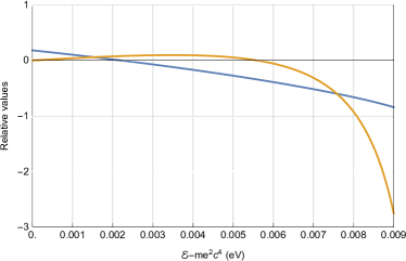
Figure 1: Numerical solution of the eigenenergies for the electron in a quantum well of $U=0.01~{}\text{e}V$ and $R=10~{}\text{nm}$.
The blue and orange curves representing $\xi J_{0}(\zeta R)K_{1}(\xi R)$ and $\frac{\mathcal{E}-U+mc^{2}}{\mathcal{E}+mc^{2}}\zeta K_{0}(\xi R)J_{1}(\zeta R)$ from Eq. 39 respectively intercept at eigenenergies $\mathcal{E}_{01}-mc^{2}=1.53(meV)$ and $7.63(meV)$ for the ground and excited state respectively.

We now calculate the ground state eigenenergies $\mathcal{E}_{01}-mc^{2}$ and $\kappa_{01}$ for all potentials, followed by the calculation of wave numbers $\zeta_{01}$ and $\xi_{01}$ with the help of Eqs. II. The results are listed in Table 1.

Table 1: Eigenenergy $\mathcal{E}_{01}$ and relative constant $\kappa_{01}$

$U$ (eV)	$\mathcal{E}_{01}-mc^{2}(meV)$	$\kappa_{01}$	$\zeta_{01}\text{(}m^{-1})$	$\xi_{01}\text{(}m^{-1})$
$0.01$	$1.53$	$44.1$	$2.00\times 10^{8}$	$4.71\times 10^{8}$
$0.10$	$1.95$	$2.23\times 10^{6}$	$2.26\times 10^{8}$	$1.60\times 10^{9}$
$1.00$	$2.12$	$2.32\times 10^{21}$	$2.36\times 10^{8}$	$5.12\times 10^{9}$
$10.0$	$2.18$	$1.75\times 10^{69}$	$2.39\times 10^{8}$	$1.62\times 10^{10}$

The numerical calculation shows that the electron wave tunnels out of the quantum well and behaves evanescent due to the characteristics of the modified Bessel functions. Fig. 2 plots the wavefunctions inside and outside the well for the ground state of $U=0.01~{}\text{e}V$. It is shown that substantial evanescent wave tunnels out of the quantum well, but satisfies wavefunction continuity at the boundary.

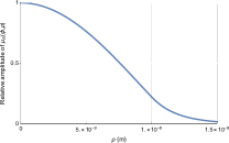
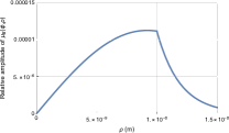
Figure 2: Wavefunction plot for the Dirac electron in a quantum well of $U=0.01~{}\text{eV}$ and $R=10~{}\text{nm}$.
The large component $\mu_{A}(\phi,\rho)$ (left) and small component $\mu_{B}(\phi,\rho)$ (right) wavefunctions demonstrate that substantial evanescent wave tunnels out of the quantum well, but satisfies wavefunction continuity at the boundary.

Table 1 shows that at higher potential, for example $U=10~{}\text{e}V$, the wave number $\zeta_{01}=2.39\times 10^{8}$ already approaches the wave number for the infinite quantum well $\zeta_{01}^{\inf}=2.40\times 10^{8}$, where zero wavefunction is assumed outside the well

$$J_{0}(\zeta_{01}^{\inf}R)=0.$$ (40)

Therefore, the wavefunctions $\mu_{A}(\phi,\rho)$ and $\mu_{B}(\phi,\rho)$ inside the quantum well are nearly the same as the wavefunctions in the infinite quantum well, as illustrated by Fig. 3. However, contrary to the conventional assumption, the wavefunctions outside the quantum well are diminished but not exactly zero, especially at the boundary for $\mu_{B}(\phi,\rho)$, so that the wavefunction continuity is always satisfied. The wavefunctions remain significant within a narrow region near the boundary known as the skin depth, but decay rapidly. The skin depth becomes narrower as the potential becomes higher, as is the case for an optical field confined in a waveguide [9].

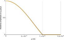
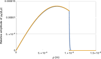
Figure 3: Wavefunction plot for the Dirac electron in a quantum well of $U=10~{}\text{eV}$ and $R=10~{}\text{nm}$.
The large component $\mu_{A}(\phi,\rho)$ (left) and small component $\mu_{B}(\phi,\rho)$ (right) wavefunctions (blue) inside the quantum well are nearly identical to the wavefunctions (orange) inside an infinite quantum well. The wavefunctions outside the quantum well are diminished but not exactly zero, especially at the boundary for $\mu_{B}(\phi,\rho)$, so that the wavefunction continuity is always satisfied.

The above analysis validates the infinite quantum well model to account for the quantum behavior of the electron inside the well. However, it also reveals that the evanescent wave diminishes but never vanishes to mathematical zero, circumventing the discontinuity problem at the boundary of the commonly-used infinite quantum well model.

IV Evanescent electron wave spin

We now investigate the spin nature of the evanescent electron wave that resides within the skin depth region outside the quantum well. Analytical expression of the current density is obtained by using the wavefunctions in Eq. 37,

$$j_{\rho} = -ec\psi^{\dagger}\alpha_{\rho}\psi=0,\textrm{e}verywhere;$$

$$j_{\phi} = -ec\psi^{\dagger}\alpha_{\phi}\psi=\biggl{\{}\begin{array}[]{ll}-\frac{e\hbar c^{2}}{\mathcal{E}+\text{m}c^{2}}\zeta J_{0}(\zeta\rho)J_{1}(\zeta\rho),&\rho\leq R\\ \\ -\kappa^{2}\frac{e\hbar c^{2}}{\mathcal{E}-U+\text{m}c^{2}}\xi K_{0}(\xi\rho)K_{1}(\xi\rho),&\rho>R,\\ \end{array}$$ (44)

where $-e=-1.602\times 10^{-19}\text{C}$ to represent the electron charge.

Eq. IV demonstrates that stable circulating current density exists both inside and outside the quantum well, as evidenced by the non-zero component $j_{\phi}$ in all regions and zero component $j_{\rho}$ everywhere. The evanescent electron wave is shown to spin concurrently with the electron wave inside the quantum well, as illustrated by the vector plot of Fig. 4. The current density continuity is observed at the boundary as a result of the wavefunction continuity at the boundary in Eqs. 35 and 37, which also ensure the charge density continuity.

The above analysis highlights the wave spin picture, in which the spin is a wave property encoded in the entire Dirac field. In other words, the evanescent wave is an integral part of the entire electron wave that possesses the wave spin property.

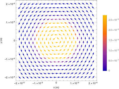
Figure 4: Vector plot of the current density for a spin-up ground state electron in a quantum well of $U=0.01~{}\text{e}V$ and $R=10~{}\text{nm}$. The evanescent wave spins concurrently with the wave inside the quantum well.

V Evanescent electron wave spin sensing

The discussion above raises questions about the security of spin quantum information and the possibility of novel evanescent electron wave spin sensing, which is analogous to evanescent optical wave sensing [8], [9], [10] that has already been employed in real applications. The evanescent optical wave is a part of an eigen electromagnetic wave outside an optic waveguide or fiber that can interact with matters around the waveguide. The main optic wave confined inside the waveguide is perturbed but largely maintained. Similarly, the evanescent electron wave is a part of an eigen electron wave outside a quantum well that can interact with an electromagnetic wave around the quantum well. The two schemes share the same fundamental matter-field interaction: $\pmb{j}(r)\cdot\pmb{A}(r)$, where $\pmb{j}(r)$ and $\pmb{A}(r)$ represent the electron wave and the electromagnetic wave, respectively. The interaction is usually small due to the nature of evanescent waves; therefore, the main wave inside the confinement is only perturbed but not destroyed. Thus, evanescent wave sensing offers a unique detection scheme as a partial wave interaction without destroying the main wave inside the confinement.

However, the evanescent electron wave contains the spin property as described by the current density $\pmb{j}(r)$ in Eq. IV. When it interacts with the electromagnetic field $\pmb{A}(r)$, only partial spin participates in the process that could result in the fractional spin effects as discussed in the previous study [5]. Such partial spin concept conflicts with the particle spin picture, where a single particle electron possesses a unit spin and can only manifest the full spin effect during interaction. In the particle electron spin picture, the electron carrying the full spin tunnels out of the quantum well with a probability density given by the square of the wavefunction $\psi^{\dagger}\psi$. If the spin is detected outside the quantum well, the spin information inside is destroyed since the electron that carries the full spin no longer exists within the quantum well.

The conflicting pictures are illustrated in Fig. 5, which comprises two figures for the electron in the same quantum well of $R=10~{}\text{nm}$ and $U=0.01~{}\text{e}V$.

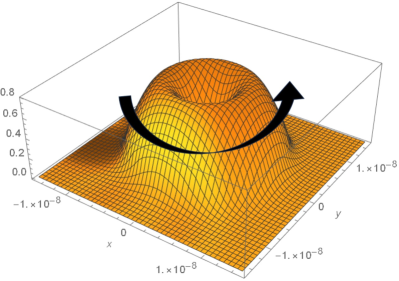
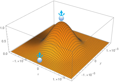
Figure 5: Conflicting views on the electron spin and tunnelling.
Upper figure illustrates the wave spin view that partial wave spin tunnels out of the quantum well with full certainty. The figure shows the three-dimension distribution of the current density that spins as a whole in all regions for the spin-up electron in a finite quantum well of $R=10~{}\text{nm}$ and $U=0.01~{}\text{e}V$.
Lower figure illustrates the particle spin view that full particle spin tunnels out of the quantum well with partial certainty. The figure shows the probability density $\psi^{\dagger}\psi$ of the particle electron of spin-up (represented by the ball and arrow) in the same quantum well.

The upper figure illustrates the wave spin picture by showing the spinning current density in all regions. The current density resembles the current density inside an infinite square well discussed previously [4]. Here, partial wave spin exists outside the quantum well but with full certainty.

The lower figure depicts the particle spin picture by showing the probability density and particle electron spin. Here, full particle spin tunnels out of the quantum well but with partial certainty.

The conflicting views reflect different interpretations of quantum mechanics, but resolving them has significant implications for emerging technology development, such as quantum computing. Quantum computing is generally regarded as a probabilistic process at the fundamental level due to the probabilistic interpretation of the wavefunction that describes the behavior of subatomic particles. By adopting the particle spin picture, which interprets spin as a local property pertaining to the particle electron, a spin-based quantum computer should also be considered as a probabilistic machine.

However, the wavefunction that is supposed to provide the probability density $\psi^{\dagger}\psi$ is deterministic itself since it is a vector in the Hilbert space. Consequently, the charge density $e\psi^{\dagger}\psi$ and current density $ec\psi^{\dagger}\alpha\psi$ are deterministic observables. We have shown that the electron spin is a wave property that can be fully described by the current density. Therefore, the electron wave spin is also a deterministic property. It is our view that a quantum process or device based on the manipulation and probing of the electron wave spin is deterministic in nature rather than probabilistic.

VI Conclusions

1. Our study shows that an evanescent electron wave exists outside both finite and infinite quantum wells, by solving exact solutions of the Dirac equation in a cylindrical quantum well and maintaining wavefunction continuity at the boundary.

2. Furthermore, we demonstrate that the evanescent wave spins concurrently with the wave inside the quantum well, by deriving analytical expressions of the current density in the whole region. Our findings suggest that it is possible to probe or eavesdrop on quantum spin information through the evanescent wave spin without destroying the entire spin state.

3. The wave spin picture interprets spin as a global and deterministic property of the electron wave that includes both the evanescent and confined wavefunctions. This suggests that a quantum process or device based on the manipulation and probing of the electron wave spin is deterministic in nature rather than probabilistic.

VII Acknowledgement

The authors would like to express their gratitude to Sumit Ghosh for the insightful discussion on the boundary condition issue of an infinite quantum well.

References

- National Academies of Sciences et al. [2019] E. National Academies of Sciences, D. Sciences, I. Board, C. Board, C. Computing, M. Horowitz, and E. Grumbling, Quantum Computing: Progress and Prospects (National Academies Press, 2019).
- Kloeffel and Loss [2013] C. Kloeffel and D. Loss, Annual Review of Condensed Matter Physics 4, 51 (2013).
- Hirohata et al. [2020] A. Hirohata, K. Yamada, Y. Nakatani, I.-L. Prejbeanu, B. Diény, P. Pirro, and B. Hillebrands, J. of Magnetism and Magnetic Materials 509, 166711 (2020).
- Gao [2022] J. Gao, J. Phys. Commun. 6, 081001 (2022).
- Gao and Shen [2023] J. Gao and F. Shen, Qeios. 10, 32388 (2023).
- Bransden and Joachain [2000] B. H. Bransden and C. J. Joachain, Quantum mechanics (2nd ed.) (Essex: Pearson Education, 2000).
- Bjorken and Drell [1964] J. D. Bjorken and S. D. Drell, Relativistic quantum mechanics, International series in pure and applied physics (McGraw-Hill, New York, NY, 1964).
- Huertas et al. [2019] C. S. Huertas, O. Calvo-Lozano, A. Mitchell, and L. M. Lechuga, Frontiers in Chemistry 7, 10.3389/fchem.2019.00724 (2019).
- Islam et al. [2023] S. Islam, B. Halder, and A. Refaie Ali, Sci. Rep. 13, 9906 (2023).
- Refaie Ali et al. [2023] A. Refaie Ali, N. Eldabe, and A. El Naby, Eur. Phys. J. Spec. Top. 10.1140/epjs/s11734- 023-00934-1 (2023).