Robust Stochastic Optimization via Gradient Quantile Clipping

Abstract

We introduce a clipping strategy for Stochastic Gradient Descent (SGD) which uses quantiles of the gradient norm as clipping thresholds. We prove that this new strategy provides a robust and efficient optimization algorithm for smooth objectives (convex or non-convex), that tolerates heavy-tailed samples (including infinite variance) and a fraction of outliers in the data stream akin to Huber contamination. Our mathematical analysis leverages the connection between constant step size SGD and Markov chains and handles the bias introduced by clipping in an original way. For strongly convex objectives, we prove that the iteration converges to a concentrated distribution and derive high probability bounds on the final estimation error. In the non-convex case, we prove that the limit distribution is localized on a neighborhood with low gradient. We propose an implementation of this algorithm using rolling quantiles which leads to a highly efficient optimization procedure with strong robustness properties, as confirmed by our numerical experiments.

1 Introduction

Stochastic gradient descent (SGD) [73] is the core optimization algorithm at the origin of most stochastic optimization procedures [45, 21, 43]. SGD and its variants are ubiquitously employed in machine learning in order to train most models [46, 6, 48, 78, 11, 55]. The convergence properties of SGD are therefore subjects of major interest. The first guarantees [62, 28] hold under strong statistical assumptions which require data to follow light-tailed sub-Gaussian distributions and provide error bounds in expectation. With the recent resurgence of interest for robust statistics [35, 23, 49, 71], variants of SGD based on clipping are shown to be robust to heavy-tailed gradients [29, 80], where the gradient samples are only required to have a finite variance. The latter requirement has been further weakened to the existence of a $q$-th moment for some $q>1$ in [77, 65]. In this paper, we go further and show that another variant of clipped SGD with proper thresholds is robust both to heavy tails and outliers in the data stream.

Robust statistics appeared in the 60s with the pioneering works of Huber, Tukey and others [81, 39, 37, 76, 30]. More recently, the field found new momentum thanks to a series of works about robust scalar mean estimation [16, 1, 42, 53] and the more challenging multidimensional case [33, 17, 52, 59, 20, 22, 50, 25]. These paved the way to the elaboration of a host of robust learning algorithms [32, 71, 49, 51, 67] which have to date overwhelmingly focused on the batch learning setting. We consider the setting of streaming stochastic optimization [10, 12, 57], which raises an additional difficulty coming from the fact that algorithms can see each sample only once and must operate under an $\mathcal{O}(d)$ memory and complexity constraint for $d$-dimensional optimization problems. A limited number of papers [80, 60, 26] propose theoretical guarantees for robust algorithms learning from streaming data.

This work introduces such an algorithm that learns from data on the fly and is robust both to heavy tails and outliers, with minimal computational overhead and sound theoretical guarantees.

We consider the problem of minimizing a smooth objective

$$\min_{\theta\in\mathbb{R}^{d}}\mathcal{L}(\theta):=\mathbb{E}_{\zeta}[\ell(\theta,\zeta)]$$ (1)

using observations $G(\theta,\zeta_{t})$ of the unknown gradient $\nabla\mathcal{L}(\theta)$, based on samples $(\zeta_{t})_{t\geq 0}$ received sequentially that include corruptions with probability $\eta<1/2$. Formulation (1) is common to numerous machine learning problems where $\ell$ is a loss function evaluating the fit of a model with parameters $\theta$ on a sample $\zeta$, the expectation $\mathbb{E}$ is w.r.t the unknown uncorrupted sample distribution.

We introduce quantile-clipped SGD (QC-SGD) which uses the iteration

$$\theta_{t+1}\!=\!\theta_{t}-\alpha_{\theta_{t}}\beta G(\theta_{t},\zeta_{t})\>\>\text{ with }\>\>\alpha_{\theta_{t}}\!=\!\min\Big{(}1,\frac{\tau_{\theta_{t}}}{\|G(\theta_{t},\zeta_{t})\|}\Big{)},$$ (2)

where $\beta>0$ is a constant step size and $\alpha_{\theta_{t}}$ is the clipping factor with threshold chosen as the $p$-th quantile $\tau_{\theta_{t}}=Q_{p}(\|\widetilde{G}(\theta_{t},\zeta_{t})\|)$ with $\widetilde{G}(\theta_{t},\zeta_{t})$ an uncorrupted sample of $\nabla\mathcal{L}(\theta_{t})$ and $p\in(0,1)$ (details will follow). Quantiles are a natural choice of clipping threshold which allows to handle heavy tails [75, 9] and corrupted data. For instance, the trimmed mean offers a robust and computationally efficient estimator of a scalar expectation [53]. Since the quantile $Q_{p}(\|\widetilde{G}(\theta_{t},\zeta_{t})\|)$ is non-observable, we introduce a method based on rolling quantiles in Section 5 which keeps the procedure $\mathcal{O}(d)$ both memory and complexity-wise.

Contributions.

Our main contributions are as follows:

• For small enough $\eta$ and well-chosen $p$, we show that, whenever the optimization objective is smooth and strongly convex, QC-SGD converges geometrically to a limit distribution such that the deviation around the optimum achieves the optimal dependence on $\eta.$

• In the non-corrupted case $\eta=0$ and with a strongly convex objective, we prove that a coordinated choice of $\beta$ and $p$ ensures that the limit distribution is sub-Gaussian with constant of order $\mathcal{O}(\sqrt{\beta}).$ In the corrupted case $\eta>0,$ the limit distribution is sub-exponential.

• For a smooth objective (non-convex) whose gradient satisfies an identifiability condition, we prove that the total variation distance between QC-SGD iterates and its limit distribution vanishes sub-linearly. In this case, the limit distribution is such that the deviation of the objective gradient is optimally controlled in terms of $\eta.$

• Finally, we provide experiments to demonstrate that QC-SGD can be easily implemented by estimating $Q_{p}(\|\widetilde{G}(\theta_{t},\zeta_{t})\|)$ with rolling quantiles. In particular, we show that the iteration is indeed robust to heavy tails and corruption on synthetic stochastic optimization tasks.

Our theoretical results are derived thanks to a modelling through Markov chains and hold under an $L_{q}$ assumption on the gradient distribution with $q>1$.

Related works.

Convergence in distribution of the Markov chain generated by constant step size SGD, relatively to the Wasserstein metric, was first established in [27]. Another geometric convergence result was derived in [87] for non-convex, non-smooth, but quadratically growing objectives, where a convergence statement relatively to a weighted total variation distance is given and a CLT is established. These papers do not consider robustness to heavy tails or outliers. Early works proposed stochastic optimization and parameter estimation algorithms which are robust to a wide class of noise of distributions [56, 68, 69, 72, 79, 19, 18, 61], where asymptotic convergence guarantees are stated for large sample sizes. Initial evidence of the robustness of clipped SGD to heavy tails was given by [88] who obtained results in expectation. Subsequent works derived high-confidence sub-Gaussian performance bounds under a finite variance assumption [29, 80] and later under an $L_{q}$ assumption [77, 65] with $q>1$.

Robust versions of Stochastic Mirror Descent (SMD) are introduced in [60, 44]. For a proper choice of the mirror map, SMD is shown to handle infinite variance gradients without any explicit clipping [85]. Finally, [26] studies heavy-tailed and outlier robust streaming estimation algorithms of the expectation and covariance. On this basis, robust algorithms for linear and logistic regression are derived. However, the involved filtering procedure is hard to implement in practice and no numerical evaluation of the considered approach is proposed.

Agenda.

In Section 2 we set notations, state the assumptions required by our theoretical results and provide some necessary background on continuous state Markov chains. In Section 3, we state our results for strongly convex objectives including geometric ergodicity of QC-SGD (Theorem 1), characterizations of the limit distribution and deviation bounds on the final estimate. In Section 4, we remove the convexity assumption and obtain a weaker ergodicity result (Theorem 2) and characterize the limit distribution in terms of the deviations of the objective gradient. Finally, we present a rolling quantile procedure in Section 5 and demonstrate its performance through a few numerical experiments on synthetic data.

2 Preliminaries

The model parameter space is $\mathbb{R}^{d}$ endowed with the Euclidean norm $\|\cdot\|$, $\mathcal{B}(\mathbb{R}^{d})$ is the Borel $\sigma$-algebra of $\mathbb{R}^{d}$ and we denote by $\mathcal{M}_{1}(\mathbb{R}^{d})$ the set of probability measures over $\mathbb{R}^{d}.$ We assume throughout the paper that the objective $\mathcal{L}$ is smooth.

Assumption 1.

The objective $\mathcal{L}$ is $L$-Lipschitz-smooth, namely

$$\mathcal{L}(\theta^{\prime})\leq\mathcal{L}(\theta)+\langle\nabla\mathcal{L}(\theta),\theta^{\prime}-\theta\rangle+\frac{L}{2}\|\theta-\theta^{\prime}\|^{2}$$

with $L<+\infty$ for all $\theta,\theta^{\prime}\in\mathbb{R}^{d}$.

The results from Section 3 below use the following

Assumption 2.

The objective $\mathcal{L}$ is $\mu$-strongly convex, namely

$$\mathcal{L}(\theta^{\prime})\geq\mathcal{L}(\theta)+\langle\nabla\mathcal{L}(\theta),\theta^{\prime}-\theta\rangle+\frac{\mu}{2}\|\theta-\theta^{\prime}\|^{2}$$

with $\mu>0$ for all $\theta,\theta^{\prime}\in\mathbb{R}^{d}$.

An immediate consequence of Assumption 2 is the existence of a unique minimizer $\theta^{\star}=\operatorname*{argmin}_{\theta\in\mathbb{R}^{d}}\mathcal{L}(\theta).$ The next assumption formalizes our corruption model.

Assumption 3 ($\eta$-corruption).

The gradients $(G(\theta_{t},\zeta_{t}))_{t\geq 0}$ used in Iteration (2) are sampled as $G(\theta_{t},\zeta_{t})=U_{t}\widecheck{G}(\theta_{t})+(1-U_{t})\widetilde{G}(\theta_{t},\zeta_{t})$ where $U_{t}$ are i.i.d Bernoulli random variables with parameter $\eta<1/2,$ $\widecheck{G}(\theta_{t})\sim\mathcal{D}_{\mathcal{O}}(\theta_{t})$ with $\mathcal{D}_{\mathcal{O}}(\theta_{t})$ an arbitrary distribution and $\widetilde{G}(\theta_{t},\zeta_{t})\sim\mathcal{D}_{\mathcal{I}}(\theta_{t})$ follows the true gradient distribution and is independent from the past given $\theta_{t}$.

Assumption 3 is an online analog of the Huber contamination model [36, 39] where corruptions occur with probability $\eta$ and where the distribution of corrupted samples is not fixed and may depend on the current iterate $\theta_{t}$. The next assumption requires the true gradient distribution to be unbiased and diffuse.

Assumption 4.

For all $\theta$, non-corrupted gradient samples $\widetilde{G}(\theta,\zeta)\sim\mathcal{D}_{\mathcal{I}}(\theta)$ are such that

$$\widetilde{G}(\theta,\zeta)=\nabla\mathcal{L}(\theta)+\varepsilon_{\theta},$$ (3)

where $\varepsilon_{\theta}$ is a centered noise $\mathbb{E}[\varepsilon_{\theta}|\theta]=0$ with distribution $\delta\nu_{\theta,1}+(1-\delta)\nu_{\theta,2}$ where $\delta>0$ and $\nu_{\theta,1},\nu_{\theta,2}$ are distributions over $\mathbb{R}^{d}$ such that $\nu_{\theta,1}$ admits a density $h_{\theta}$ w.r.t. the Lebesgue measure satisfying

$$\inf_{\|\omega\|\leq R}h_{\theta}(\omega)>\varkappa(R)>0$$

for all $R>0$, where $\varkappa(\cdot)$ is independent of $\theta.$

Assumption 4 imposes a weak constraint, since it is satisfied, for example, as soon as the noise $\varepsilon_{\theta}$ admits a density w.r.t. Lebesgue’s measure. Our last assumption formalizes the requirement of a finite moment for the gradient error.

Assumption 5.

There is $q>1$ such that for $\widetilde{G}(\theta,\zeta)\sim\mathcal{D}_{\mathcal{I}}(\theta),$ we have

$$\mathbb{E}\big{[}\|\varepsilon_{\theta}\|^{q}\>|\>\theta\big{]}^{1/q} =\mathbb{E}\big{[}\big{\|}\widetilde{G}(\theta,\zeta)-\nabla\mathcal{L}(\theta)\big{\|}^{q}\>|\>\theta\big{]}^{1/q}\leq A_{q}\|\theta-\theta^{\star}\|+B_{q}$$ (4)

for all $\theta\in\mathbb{R}^{d},$ where $A_{q},B_{q}>0$. When $\mathcal{L}$ is not strongly convex, we further assume that $A_{q}=0.$

The bound (4) captures the case of arbitrarily high noise magnitude through the dependence on $\|\theta-\theta^{\star}\|.$ This is consistent with common strongly convex optimization problems such as least squares regression. For non-strongly convex $\mathcal{L}$, we require $A_{q}=0$ since $\theta^{\star}$ may not exist.

Definition 1.

If $X$ is a real random variable, we say that $X$ is $K$-sub-Gaussian for $K>0$ if

$$\mathbb{E}\exp(\lambda^{2}X^{2})\leq e^{\lambda^{2}K^{2}}\quad\text{for}\quad|\lambda|\leq 1/K.$$ (5)

We say that $X$ is $K$-sub-exponential for $K>0$ if

$$\mathbb{E}\exp(\lambda|X|)\leq\exp(\lambda K)\quad\text{ for all}\quad 0\leq\lambda\leq 1/K.$$ (6)

The convergence results presented in this paper use the following formalism of continuous state Markov chains. Given a step size $\beta>0$ and a quantile $p\in(0,1),$ we denote by $P_{\beta,p}$ the Markov transition kernel governing the Markov chain $(\theta_{t})_{t\geq 0}$ generated by QC-SGD, so that

$$\mathbb{P}(\theta_{t+1}\in A\>|\>\theta_{t})=P_{\beta,p}(\theta_{t},A)$$

for $t\geq 0$ and $A\in\mathcal{B}(\mathbb{R}^{d})$. The transition kernel $P_{\beta,p}$ acts on probability distributions $\nu\in\mathcal{M}_{1}(\mathbb{R}^{d})$ through the mapping $\nu\to\nu P_{\beta,p}$ which is defined, for all $A\in\mathcal{B}(\mathbb{R}^{d})$, by $\nu P_{\beta,p}(A)=\int_{A}P_{\beta,p}(\theta,A)d\nu(\theta)=\mathbb{P}(\theta_{t+1}\in A\>|\>\theta_{t}\sim\nu).$ For $n\geq 1,$ we similarly define the multi-step transition kernel $P_{\beta,p}^{n}$ which is such that $P^{n}_{\beta,p}(\theta_{t},A)=\mathbb{P}(\theta_{t+n}\in A\>|\>\theta_{t})$ and acts on probability distributions $\nu\in\mathcal{M}_{1}(\mathbb{R}^{d})$ through $\nu P_{\beta,p}^{n}=(\nu P_{\beta,p})P_{\beta,p}^{n-1}.$ Finally, we define the total variation (TV) norm of a signed measure $\nu$ as

$$2\|\nu\|_{\operatorname{TV}} =\sup_{f:|f|\leq 1}\int f(\theta)\nu(d\theta)=\sup_{A\in\mathcal{B}(\mathbb{R}^{d})}\nu(A)-\inf_{A\in\mathcal{B}(\mathbb{R}^{d})}\nu(A).$$

In particular, we recover the TV distance between $\nu_{1},\nu_{2}\in\mathcal{M}_{1}(\mathbb{R}^{d})$ as $d_{\operatorname{TV}}(\nu_{1},\nu_{2})=\|\nu_{1}-\nu_{2}\|_{\operatorname{TV}}.$

3 Strongly Convex Objectives

We are ready to state our convergence result for the stochastic optimization of a strongly convex objective using QC-SGD with $\eta$-corrupted samples.

Theorem 1 (Geometric ergodicity).

Let Assumptions 1-5 hold and assume there is a quantile $p\in[\eta,1-\eta]$ such that

$$\kappa:=(1-\eta)p\mu-\eta L-(1-p)^{-\frac{1}{q}}A_{q}(1-p(1-\eta))>0.$$ (7)

Then, for a step size $\beta$ satisfying

$$\beta<\frac{1}{4}\frac{\kappa}{\mu^{2}+6L^{2}+16\eta^{-\frac{2}{q}}A_{q}^{2}},$$ (8)

the Markov chain $(\theta_{t})_{t\geq 0}$ generated by QC-SGD with parameters $\beta$ and $p$ converges geometrically to a unique invariant measure $\pi_{\beta,p}$: for any initial $\theta_{0}\in\mathbb{R}^{d},$ there is $\rho<1$ and $M<\infty$ such that after $T$ iterations

$$\big{\|}\delta_{\theta_{0}}P_{\beta,p}^{T}-\pi_{\beta,p}\big{\|}_{\operatorname{TV}}\leq M\rho^{T}\big{(}1+\|\theta_{0}-\theta^{\star}\|^{2}\big{)},$$

where $\delta_{\theta_{0}}$ is the Dirac measure located at $\theta_{0}.$

The proof of Theorem 1 is given in Appendix C.2 and relies on the geometric ergodicity result of [58, Chapter 15] for Markov chains with a geometric drift property. A similar result for quadratically growing objectives was established by [87] and convergence w.r.t. Wasserstein’s metric was shown in [27] assuming uniform gradient co-coercivity. However, robustness was not considered in these works. The restriction $p\in[\eta,1-\eta]$ comes from the consideration that other quantiles are not estimable in the event of $\eta$-corruption. Condition (7) is best interpreted for the choice $p=1-\eta$ in which case it translates into $\eta^{1-{1/q}}\leq\mathcal{O}(\mu/(L+A_{q}))$ implying that it is verified for $\eta$ small enough within a limit fixed by the problem conditioning. A similar condition with $q=2$ appears in [26, Theorem E.9] which uses a finite variance assumption.

The constants $M$ and $\rho$ controlling the geometric convergence speed in Theorem 1 depend on the parameters $\beta,p$ and the initial $\theta_{0}.$ Among choices fulfilling the convergence conditions, it is straightforward that greater step size $\beta$ and $\theta_{0}$ closer to $\theta^{\star}$ lead to faster convergence. However, the dependence in $p$ is more intricate and should be evaluated through the resulting value of $\kappa$. We provide a more detailed discussion about the value of $\rho$ in Appendix B.

The choice $p=1-\eta$ appears to be ideal since it leads to optimal deviation of the invariant distribution around the optimum $\theta^{\star}$ which is the essence of our next statement.

Proposition 1.

Assume the same as in Theorem 1 and condition (7) with the choice $p=1-\eta$. For step size $\beta$ satisfying (8), $q\geq 2$, and additionally:

$$\beta\leq{\eta^{2-2/q}/\kappa},$$ (9)

for $\theta\sim\pi_{\beta,1-\eta}$, we have the following upper bound:

$$\mathbb{E}\|\theta-\theta^{\star}\|^{2}\leq\Big{(}\frac{6\eta^{1-1/q}B_{q}}{\kappa}\Big{)}^{2}.$$

Proposition 1 is proven in Appendix C.3. An analogous result holds for $q\in(1,2)$ but requires a different proof and can be found in Appendix C.4. Proposition 1 may be compared to [87, Theorem 3.1] which shows that the asymptotic estimation error can be reduced arbitrarily using a small step size. However, this is impossible in our case since we consider corrupted gradients. The performance of Proposition 1 is best discussed in the specific context of linear regression where gradients are given as $G(\theta,(X,Y))=X(X^{\top}\theta-Y)$ for samples $X,Y\in\mathbb{R}^{d}\times\mathbb{R}$ such that $Y=X^{\top}\theta^{\star}+\epsilon$ with $\epsilon$ a centered noise. In this case, a finite moment of order $k$ for the data implies order $k/2$ for the gradient corresponding to an $\eta^{1-2/k}$ rate in Proposition 1. Since Assumption 5 does not include independence of the noise $\epsilon$ from $X,$ this corresponds to the negatively correlated moments assumption of [2] being unsatisfied. Consequently, Proposition 1 is information-theoretically optimal in $\eta$ based on [2, Corollary 4.2]. Nonetheless, the poor dimension dependence through $B_{q}$ may still be improved. If the gradient is sub-Gaussian with constant $K$, we would have $B_{q}\lesssim K\sqrt{q}$ for $q\geq 1$ (see [83] for a reference), in which case, the choice $q=\log(1/\eta)$ recovers the optimal rate in $\eta\sqrt{\log(1/\eta)}$ for the Gaussian case.

We now turn to showing strong concentration properties for the invariant distribution $\pi_{\beta,p}.$ For this purpose, we restrict the optimization to a bounded and convex set $\Theta\subset\mathbb{R}^{d}$ and replace Iteration (2) by the projected iteration

$$\theta_{t+1}=\Pi_{\Theta}\big{(}\theta_{t}-\alpha_{\theta_{t}}\beta G(\theta_{t},\zeta_{t})\big{)},$$ (10)

where $\Pi_{\Theta}$ is the projection onto $\Theta$. Assuming that the latter contains the optimum $\theta^{\star}\in\Theta,$ one can check that the previous results continue to hold thanks to the inequality

$$\|\Pi_{\Theta}(\theta)-\theta^{\star}\|=\|\Pi_{\Theta}(\theta)-\Pi_{\Theta}(\theta^{\star})\|\leq\|\theta-\theta^{\star}\|,$$

which results from the convexity of $\Theta.$ The restriction of the optimization to a bounded set allows us to uniformly bound the clipping threshold $\tau_{\theta}$, which is indispensable for the following result.

Proposition 2.

In the setting of Theorem 1, consider projected QC-SGD (10) and let $\overline{\tau}=\sup_{\theta\in\Theta}\tau_{\theta},D=\operatorname{diam}(\Theta)$ the diameter of $\Theta$ and $\overline{B}_{q}=A_{q}D+B_{q}.$

• Consider the non-corrupted case $\eta=0$ and set the quantile $p$ such that $p\geq 1-(\beta\mu)^{\frac{q}{2(q-1)}}.$ Then, for $\theta\sim\pi_{\beta,p},$ the variable $\|\theta-\theta^{\star}\|$ is sub-Gaussian in the sense of Definition 1 with constant

  $$K=4\sqrt{\frac{2\beta(\overline{B}_{q}^{2}+\overline{\tau}^{2})}{p\mu}}.$$

• Consider the corrupted case $\eta>0,$ and set the quantile $p\in[\eta,1-\eta]$ such that Inequality (7) holds. Then, for $\theta\sim\pi_{\beta,p},$ the variable $\|\theta-\theta^{\star}\|$ is sub-exponential in the sense of Definition 1 with constant

  $$K=\frac{7\overline{\tau}+(1-p)^{1-1/q}\overline{B}_{q}}{p\mu}.$$

The proof can be found in Appendix C.5. The strong concentration properties given by Proposition 2 for the invariant distribution appear to be new. Still, the previous result remains asymptotic in nature. High confidence deviation bounds for an iterate $\theta_{t}$ can be derived by leveraging the convergence in Total Variation distance given by Theorem 1 leading to the following result.

Corollary 1.

In the setting of Proposition 2, in the absence of corruption $\eta=0,$ after $T$ iterations, for $\delta>0,$ we have

$$\mathbb{P}\bigg{(}\big{\|}\theta_{T}-\theta^{\star}\big{\|}>4\sqrt{\overline{B}_{q}^{2}+\overline{\tau}^{2}} \sqrt{\frac{2\beta\log(e/\delta)}{p\mu}}\bigg{)}\leq\delta+\rho^{T}M\big{(}1+\|\theta_{0}-\theta^{\star}\|^{2}\big{)}.$$

Choosing a smaller step size $\beta$ in Corollary 1 allows to improve the deviation bound. However, this comes at the cost of weaker confidence because of slower convergence due to a greater $\rho.$ See Appendix B for a discussion including a possible compromise. Corollary 1 may be compared to the results of [29, 80, 77, 65] which correspond to $\beta\approx 1/T$ and have a similar dependence on the dimension through the gradient variance. Although their approach is also based on gradient clipping, they use different thresholds and proof methods. In the presence of corruption, the invariant distribution is not sub-Gaussian. This can be seen by considering the following toy Markov chain:

$$X_{t+1}=\begin{cases}\alpha X_{t}+\xi&\text{w.p.}\quad 1-\eta\\ X_{t}+\tau&\text{w.p.}\quad\eta\end{cases}$$

where $\alpha<1,\tau>0$ are constants and $\xi$ is a positive random noise. Using similar methods to the proof of Theorem 1, one can show that $(X_{t})_{t\geq 0}$ converges (for any initial $X_{0}$) to an invariant distribution whose moments can be shown to grow linearly, indicating a sub-exponential distribution and excluding a sub-Gaussian one. We provide additional details for the underlying argument in Appendix C.6. For the corrupted case, the sub-exponential property stated in Proposition 2 holds with a constant $K$ of order $\overline{\tau}/\mu$, which is not satisfactory and leaves little room for improvement due to the inevitable bias introduced by corruption. Therefore, we propose the following procedure in order to obtain a high confidence estimate, similarly to Corollary 1.

Input: Step size $\beta>0$, quantile index $p\in(0,1)$, initial parameter $\theta_{0}\in\Theta$, horizon $T$ and

number of concurrent iterates $N\geq 1.$

Optimize multiple parameters $\theta^{(1)}_{t},\dots,\theta^{(N)}_{t}$ starting from a common $\theta_{0}=\theta^{(n)}_{0}$ for $n\in\llbracket N\rrbracket=:\{1,\ldots,N\}$ and $T$ steps $t=0,\ldots,T$ using the following cycling iteration:

$$\theta^{(n)}_{t+1}\!=\!\begin{cases}\theta^{(n)}_{t}\!-\!\alpha_{\theta^{(n)}_{t}}\beta G\big{(}\theta^{(n)}_{t},\zeta_{t}\big{)}&\text{ if }t\!\equiv\!n\!-\!1\bmod N,\\ \theta^{(n)}_{t}&\text{ otherwise.}\end{cases}$$ (11)

Compute $r_{ij}=\big{\|}\theta_{T}^{(i)}-\theta_{T}^{(j)}\big{\|}$ for $i,j\in\llbracket N\rrbracket.$

For $j\!\in\!\llbracket N\rrbracket$, let $r^{(j)}\!\in\!\mathbb{R}_{+}^{N}$ be the vector $r_{j,:}\!:=\![r_{j,1},\ldots,r_{j,N}]$ sorted in non decreasing order.

Compute the aggregated estimator as $\widehat{\theta}=\theta_{T}^{(\widehat{i})}$ with $\widehat{i}=\operatorname*{argmin}_{i\in\llbracket N\rrbracket}r^{(i)}_{N/2}.$

return $\widehat{\theta}$

Algorithm 1 Aggregation of cycling iterates

Algorithm 1 uses ideas from [35] (see also [59, 44]) and combines a collection of weak estimators (only satisfying $L_{2}$ bounds) into a strong one with sub-exponential deviation. The aggregated estimator $\widehat{\theta}$ satisfies the high probability bound given in the next result.

Corollary 2.

Assume the same as in Theorem 1 and Proposition 1. Consider $\widehat{\theta}$ given by Algorithm 1, with the assumption that the gradient sample sets used for each $\big{(}\theta_{T}^{(n)}\big{)}_{n\in\llbracket N\rrbracket}$ in Equation (11) are independent. For $\delta>0,$ if $N\geq 16\log(1/\delta)$ and $T$ satisfies

$$T\geq N\log(15M(1+\|\theta_{0}-\theta^{\star}\|^{2}))/\log(1/\rho),$$

then, with probability at least $1-\delta,$ we have

$$\big{\|}\widehat{\theta}-\theta^{\star}\big{\|}\leq\frac{27\eta^{1-\frac{1}{q}}\overline{B}_{q}}{\kappa}.$$ (12)

We obtain a high confidence version of the bound in expectation previously stated in Proposition 1. As argued before, the above bound depends optimally on $\eta.$ Similar bounds to (12) are obtained for $q=2$ in [26] for streaming mean estimation, linear and logistic regression. Their results enjoy better dimension dependence but are less general than ours. In addition, the implementation of the associated algorithm is not straightforward whereas our method is quite easy to use (see Section 5).

4 Smooth Objectives

In this section, we drop Assumption 2 and consider the optimization of possibly non-convex objectives. Consequently, the existence of a unique optimum $\theta^{\star}$ and the quadratic growth of the objective are no longer guaranteed. This motivates us to use a uniform version of Assumption 5 with $A_{q}=0$ since the gradient is no longer assumed coercive and its deviation moments can be taken as bounded. In this context, we obtain the following weaker (compared to Theorem 1) ergodicity result for QC-SGD.

Theorem 2 (Ergodicity).

Let Assumptions 1, 3, 4 and 5 hold with $A_{q}=0$ (uniformly bounded moments) and positive objective $\mathcal{L}$. Let $(\theta_{t})_{t\geq 0}$ be the Markov chain generated by QC-SGD with step size $\beta$ and quantile $p\in[\eta,1-\eta]$. Assume that $p$ and $\beta$ are such that $3p(1-\eta)/4>L\beta+\eta$ and that the subset of $\mathbb{R}^{d}$ given by

$$\Big{\{}\theta:\frac{1}{2}\big{\|}\nabla\mathcal{L}(\theta)\big{\|}^{2}\!\leq\!\frac{B_{q}^{2}\big{(}(1\!-\!p)^{-\frac{2}{q}}(L\beta\!+\!2\eta^{2})\!+\!2\eta^{2-\frac{2}{q}}\big{)}}{p(1\!-\!\eta)(3p(1\!-\!\eta)/4\!-\!L\beta\!-\!\eta)}\Big{\}}$$ (13)

is bounded. Then, for any initial $\theta_{0}\in\mathbb{R}^{d},$ there exists $M<+\infty$ such that after $T$ iterations

$$\big{\|}\delta_{\theta_{0}}P_{\beta,p}^{T}-\pi_{\beta,p}\big{\|}_{\operatorname{TV}}\leq\frac{M}{T},$$ (14)

where $\pi_{\beta,p}$ is a unique invariant measure and where $\delta_{\theta_{0}}$ is the Dirac measure located at $\theta_{0}.$

The proof is given in Appendix C.9 and uses ergodicity results from [58, Chapter 13]. Theorem 2 provides convergence conditions for an SGD Markov chain on a smooth objective in a robust setting. We are unaware of anterior results of this kind in the literature. Condition (13) requires that the true gradient exceeds the estimation error at least outside of a bounded set. If this does not hold, the gradient would be dominated by the estimation error, leaving no hope for the iteration to converge. Observe that, for no corruption ($\eta=0$), the condition is always fulfilled for some $\beta$ and $p$. Note also that without strong convexity (Assumption 2), convergence occurs at a slower sublinear rate which is consistent with the optimization rate expected for a smooth objective (see  [13, Theorem 3.3]).

As previously, we complement Theorem 1 with a characterization of the invariant distribution.

Proposition 3.

Under the conditions of Theorem 2, assume that the choice $p=1-\eta$ is such that the set (13) is bounded. For step size $\beta\leq\eta^{2}/L,$ the stationary measure $\theta\sim\pi_{\beta,1-\eta}$ satisfies

$$\mathbb{E}\big{\|}\nabla\mathcal{L}(\theta)\big{\|}^{2}\leq\frac{5\eta^{2-\frac{2}{q}}B_{q}^{2}}{p(1-\eta)\big{(}3p(1-\eta)/4-L\beta-\eta\big{)}}.$$ (15)

The statement of Proposition 3 is clearly less informative than Propositions 1 and 2 since it only pertains to the gradient rather than, for example, the excess risk. This is due to the weaker assumptions that do not allow to relate these quantities. Still, the purpose remains to find a critical point and is achieved up to $\mathcal{O}(\eta^{1-1/q})$ precision according to this result. Due to corruption, the estimation error on the gradient cannot be reduced beyond $\Omega(\eta^{1-{1/q}})$ [70, 34, 24]. Therefore, one may draw a parallel with a corrupted mean estimation task, in which case, the previous rate is, in fact, information-theoretically optimal.

5 Implementation and Numerical Experiments

The use of the generally unknown quantile $Q_{p}(\|\widetilde{G}(\theta_{t},\zeta_{t})\|)$ in QC-SGD constitutes the main obstacle to its implementation. For strongly convex objectives, one may use a proxy such as $a\|\theta_{t}-\theta_{\mathrm{ref}}\|+b$ with positive $a,b$ and $\theta_{\mathrm{ref}}\in\mathbb{R}^{d}$ an approximation of $\theta^{\star}$ serving as reference point. This choice is consistent with Assumptions 1 and 5, see Lemma 2 in Appendix C.

Input: Step size $\beta>0$, quantile index

$p\in(0,1)$, initial parameter $\theta_{0}\in\mathbb{R}^{d}$, $\tau_{\mathrm{unif}}>0$, buffer $B$ of size $S$ and horizon $T.$

Fill $B$ with $S-1$ values equal to $\tau_{\mathrm{unif}}$.

for $t=0\dots T-1$ do

       Draw a sample $G(\theta_{t},\zeta_{t})$ and add $\|G(\theta_{t},\zeta_{t})\|$ to $B.$

       $\widehat{Q}_{p}\leftarrow\lfloor pS\rfloor$ rank element of $B$.

       $\theta_{t+1}\leftarrow\theta_{t}-\beta\mathrm{clip}(G(\theta_{t},\zeta_{t}),\widehat{Q}_{p})$

       Delete the oldest value in $B$.

      

end for

return $\theta_{T}$

Algorithm 2 Rolling QC-SGD

In the non-strongly convex case, a constant threshold can be used since the gradient is a priori uniformly bounded, implying the same for the quantiles of its deviations. In practice, we propose a simpler and more direct approach: we use a rolling quantile procedure, described in Algorithm 2. The latter stores the values $(\|G(\theta_{t-j},\zeta_{t-j})\|)_{1\leq j\leq S}$ in a buffer of size $S\in\mathbb{N}^{*}$ and replaces $Q_{p}(\|\widetilde{G}(\theta_{t},\zeta_{t})\|)$ in QC-SGD by an estimate $\widehat{Q}_{p}$ which is the $\lfloor pS\rfloor$-th order statistic in the buffer. Note that only the norms of previous gradients are stored in the buffer, limiting the memory overhead to $\mathcal{O}(S)$. The computational cost of $\widehat{Q}_{p}$ can also be kept to $\mathcal{O}(S)$ per iteration thanks to a bookkeeping procedure (see Appendix A).

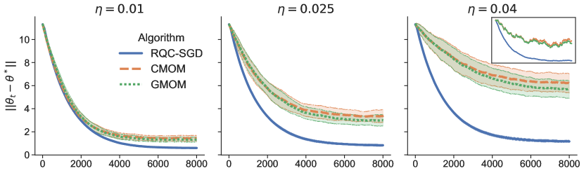
Figure 1: Evolution of $\|\theta_{t}-\theta^{\star}\|$ ($y$-axis) against iteration $t$ ($x$-axis) for the expectation estimation task, averaged over 100 runs at different corruption levels $\eta$ (bands widths correspond to the standard deviation of the 100 runs). For $\eta=0.04,$ the evolution on a single run is also displayed. We observe good performance for RQC-SGD for increasing $\eta$ while CMOM and GMOM are more sensitive.

We implement this procedure for a few tasks and compare its performance with relevant baselines. We do not include a comparison with [26] whose procedure has no implementation we are aware of and is difficult to use in practice due to its dependence on a number of unknown constants. All our experiments consider an infinite horizon, dimension $d=128$, and a constant step size for all methods.

Expectation estimation.

We estimate the expectation of a random vector $X$ by minimizing the objective $\mathcal{L}(\theta)=\frac{1}{2}\|\theta-\theta^{\star}\|^{2}$ with $\theta^{\star}=\mathbb{E}[X]$ using a stream of both corrupted and heavy-tailed samples, see Appendix A for details. We run RQC-SGD (Algorithm 2) and compare it to an online version of geometric and coordinate-wise Median-Of-Means (GMOM and CMOM) [14, 15] which use block sample means to minimize an $L_{1}$ objective (see Appendix A). Although these estimators are a priori not robust to $\eta$-corruption, we ensure that their estimates are meaningful by limiting $\eta$ to $4\%$ and using blocks of $10$ samples. Thus, blocks are corrupted with probability $<1/2$ so that the majority contains only true samples. Figure 1 displays the evolution of $\|\theta_{t}-\theta^{\star}\|$ for each method averaged over 100 runs for increasing $\eta$ and constant step size. We also display a single run for $\eta=0.04$. We observe that RQC-SGD is only weakly affected by the increasing corruption whereas the performance of GMOM and CMOM quickly degrades with $\eta$, leading to unstable estimates.

Linear regression.

We consider least-squares linear regression and compare RQC-SGD with Huber’s estimator [38] and clipped SGD (designated as CClip($\lambda$)) with three clipping levels $\lambda\sigma_{\max}\sqrt{d}$ for $\lambda\in\{0.8,1.0,1.2\}$ where $\sigma_{\max}$ is a fixed data scaling factor. These thresholds provide a rough estimate of the gradient norm. We generate covariates $X$ and labels $Y$ both heavy-tailed and corrupted. Corruption in the data stream is generated according to Assumption 3 with outliers represented either by aberrant values or fake samples $Y=X^{\top}\theta_{\mathrm{fake}}+\epsilon$ using a false parameter $\theta_{\mathrm{fake}}$, see Appendix A for further details on data generation and fine tuning of the Huber parameter. All methods are run with constant step size and averaged results over $100$ runs are displayed on Figure 2 (top row).

As anticipated, Huber’s loss function is not robust to corrupted covariates. In contrast, using gradient clipping allows convergence to meaningful estimates. Although this holds true for a constant threshold, Figure 2 shows it may considerably slow the convergence if started away from the optimum. In addition, the clipping level also affects the final estimation precision and requires tuning. Both of the previous issues are well addressed by RQC-SGD whose adaptive clipping level allows fast progress of the optimization and accurate convergence towards a small neighborhood of the optimum.

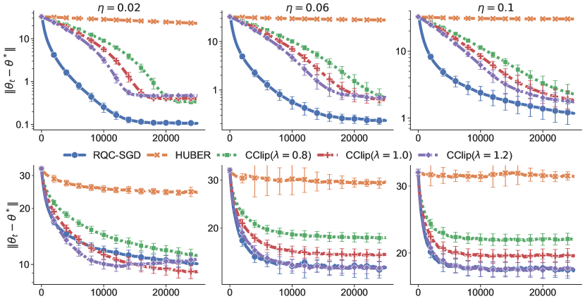
Figure 2: Evolution of $\|\theta_{t}-\theta^{\star}\|$ on the tasks of linear regression (top row) and logistic regression (bottom row) averaged over 100 runs at increasing corruption levels (error bars represent half the standard deviation). Estimators based on Huber’s loss are strongly affected by data corruption. SGD with constant clipping thresholds is robust but slow to converge for linear regression and requires tuning for better final precision. RQC-SGD combines fast convergence with good final precision thanks to its adaptive clipping strategy.

Logistic regression.

Finally, we test the same methods on logistic regression. Huber’s baseline is represented by the modified Huber loss (also known as quadratic SVM [89]). We generate data similarly to the previous task except for the labels which follow $Y\sim\operatorname{Bernoulli}(\sigma(X^{\top}\theta^{\star}))$ with $\sigma$ the sigmoid function. Corrupted labels are either uninformative, flipped or obtained with a fake $\theta_{\mathrm{fake}}$ (see details in Appendix A). Results are displayed on the bottom row of Figure 2.

As previously, Huber’s estimator performs poorly with corruption. However, constant clipping appears to be better suited when the gradient is bounded, so that the optimization is less affected by its underestimation. We observe, nonetheless, that a higher clipping level may lead to poor convergence properties, even at a low corruption rate. Note also that the constant levels we use are based on prior knowledge about the data distribution and would have to be fine tuned in practice. Meanwhile, the latter issue is well addressed by quantile clipping. Finally, notice that no algorithm truly approaches the true solution for this task. This reflects the difficulty of improving upon Proposition 3 which only states convergence to a neighborhood where the objective gradient is comparable to the estimation error in magnitude.

6 Conclusion

We introduced a new clipping strategy for SGD and proved that it defines a stochastic optimization procedure which is robust to both heavy tails and outliers in the data stream. We also provided an efficient rolling quantile procedure to implement it and demonstrated its performance through numerical experiments on synthetic data. Future research directions include improving the dimension dependence in our bounds, possibly by using sample rejection rules or by considering stochastic mirror descent [63, 4] clipped with respect to a non Euclidean norm. This may also procure robustness to higher corruption rates. Another interesting research track is the precise quantification of the geometric convergence speed of the Markov chain generated by constant step size SGD on a strongly convex objective.

Acknowledgements

This research is supported by the Agence Nationale de la Recherche as part of the “Investissements d’avenir” program (reference ANR-19-P3IA-0001; PRAIRIE 3IA Institute).

Supplementary Material

Robust Stochastic Optimization via Gradient Quantile Clipping

Appendix A Experimental details

As previously mentioned, the dimension is set to $d=128$ in all our experiments. We also set $\sigma_{\min}=1$ and $\sigma_{\max}=5$ as minimum and maximum scaling factors. For all tasks and algorithms, the optimization starts from $\theta_{0}=0.$

Bookkeeping in RQC-SGD

The buffer in Algorithm 2 stores values in sorted order along with their “ages”. The most recent and oldest values have ages $0$ and $S-1$ respectively. At each iteration, a new gradient is received, all ages are incremented and the oldest value is replaced by the new one with age $0.$ The latter is then sorted using one iteration of insertion sort. The estimate $\widehat{Q}_{p}$ is retrieved at each iteration as the value at position $\lfloor pS\rfloor.$

A.1 Mean estimation

Data generation

We compute a matrix $\Sigma=(AA^{\top}+A^{\top}A)/2$ where $A\in\mathbb{R}^{d\times d}$ is a random matrix with i.i.d centered Gaussian entries with variance $1/d$ sampled once and for all. We generate true samples as $X=\mathbf{1}+\Sigma V$ where $V$ is a vector of i.i.d symmetrized Pareto random variables with parameter $2$ and $\mathbf{1}\in\mathbb{R}^{d}$ denotes the vector with all entries equal to $1.$

We draw corrupted samples as $\widecheck{X}=10\widecheck{V}-100\times\mathbf{1}$ where $\widecheck{V}$ is a vector of i.i.d symmetrized Pareto variables with parameter $1.5.$ We use step size $\beta=10^{-3}.$

GMOM and CMOM

The geometric and coordinatewise Median-Of-Means estimators (GMOM and CMOM) optimize the following objectives respectively:

$$\mathbb{E}\big{\|}\theta-\overline{X}_{N_{b}}\|_{2}\quad\text{and}\quad\mathbb{E}\big{\|}\theta-\overline{X}_{N_{b}}\big{\|}_{1},$$

where $\overline{X}_{N_{b}}$ is the average of $N_{b}$ independent copies of $X.$ The block size is set to $N_{b}=10$ in the whole experiment. The above objectives are optimized by computing samples of $\overline{X}_{N_{b}}$ in a streaming fashion so that one step is made for each ${N_{b}}$ samples. In order to compensate for this inefficiency we multiply the step size by $N_{b}$ for both GMOM and CMOM. For GMOM, we additionally multiply the step size by $\sqrt{d}$ in order to compensate the normalization included in the gradient formula.

RQC-SGD

For mean estimation, we implement RQC-SGD (Algorithm 2) with buffer size $S=100,p=0.2$ and $\tau_{\mathrm{unif}}=10.$

A.2 Linear regression

Data generation

We choose the true parameter $\theta^{\star}$ by independently sampling its coordinate uniformly in the interval $[-5,+5].$ The true covariates are sampled as $X=\Sigma V$ where $\Sigma$ is a diagonal matrix with entries sampled uniformly in the interval $[\sigma_{\min},\sigma_{\max}]$ (once and for all) and $V$ is a vector of i.i.d symmetrized Pareto random variables with parameter $2.$ The labels are sampled as $Y=X^{\top}\theta^{\star}+\epsilon$ where $\epsilon$ is a symmetrized Pareto random variable with parameter $2.$

The corrupted samples are obtained according to one of the following possibilities with equal probability:

• $X=1000(\max_{i}\Sigma_{ii})v+W$ where $v$ is a fixed unit vector and $W$ is a standard Gaussian vector and $Y\sim\operatorname{Bernoulli}(1/2).$

• $X=1000(\max_{i}\Sigma_{ii})V$ with $V$ a unit norm random vector with uniform distribution and $Y=1000(Z+U)$ where $Z$ is a random sign and $U$ is uniform over $[-1/5,1/5].$

• $X=10V$ with $V$ a random vector with i.i.d entries following a symmetrized Log-normal distribution and $Y=X^{\top}\theta_{\mathrm{fake}}+\epsilon$ with $\theta_{\mathrm{fake}}$ a fake parameter drawn similarly to $\theta^{\star}$ once and for all and $\epsilon$ a standard Gaussian variable.

We use step size $\beta=10^{-3}.$

Huber parameter

In order to tune the parameter $\delta$ of Huber’s loss function, we proceed as follows:

• For each corruption level $\eta,$ we consider $10$ candidate values $\delta_{j}=10^{j/2-5}$ for $0\leq j<10.$

• For each candidate $\delta_{j}$, we train $250$ estimators $\big{(}\widehat{\theta}_{\delta_{j}}^{(i)}\big{)}_{i\in\llbracket 250\rrbracket}$ using $1000$ samples each.

• We choose $\widehat{j}$ for which the average $\frac{1}{250}\sum_{i\in\llbracket 250\rrbracket}\big{\|}\widehat{\theta}_{\delta_{j}}^{(i)}-\theta^{\star}\big{\|}$ is minimal and use $\widehat{\delta}=\delta_{\widehat{j}}$ as parameter.

RQC-SGD

For linear regression, we run RQC-SGD with buffer size $S=100$ and $\tau_{\mathrm{unif}}=10.$ The quantile value was set to $p=0.1$ for $\eta\in\{0.02,0.06\}$ and $p=0.05$ for $\eta=0.1$.

A.3 Logistic regression

Data generation

The true parameter $\theta^{\star}$ and covariates $X$ are chosen similarly to linear regression. Given $X$, the label $Y$ is set to $+1$ with probability $\sigma(X^{\top}\theta^{\star})$ where $\sigma$ is the sigmoid function $\sigma(x)=(1+e^{-x})^{-1}$ and to $-1$ otherwise.

The corrupted covariates are determined similarly to linear regression while the labels are set as follows in each respective case:

• $Y$ is set to $+1$ or $-1$ with equal probability.

• $Y=-\operatorname{sign}(X^{\top}\theta^{\star}).$

• $Y=\operatorname{sign}(X^{\top}\theta_{\mathrm{fake}})$ with $\theta_{\mathrm{fake}}$ a fake parameter drawn similarly to $\theta^{\star}$ once and for all.

We use step size $\beta=6\times 10^{-3}.$

Huber parameter

The same procedure is used to tune the parameter of the modified Huber loss as for linear regression.

RQC-SGD

For logistic regression, we run RQC-SGD with buffer size $S=100$ and $\tau_{\mathrm{unif}}=10$. The quantile value was set to $p=1-\eta-0.1$ for $\eta=0.02$ and $p=1-\eta-0.05$ otherwise.

A.4 Used assets

We implemented our experiments using python and a number of its libraries listed below along with their licenses:

• matplotlib (3.3.4) [40], license: https://github.com/matplotlib/matplotlib/blob/master/LICENSE/LICENSE

• numba (0.51.2) [47], BSD 2-Clause “Simplified” License

• numpy (1.19.2) [31], BSD-3-Clause License

• pandas (1.3.4) [66], BSD-3-Clause License

• python (3.8.5) [82], Python Software Foundation Licence version 2

• scipy (1.6.1) [84], BSD 3-Clause License

• seaborn (0.12.2) [86], BSD-3-Clause License

All experiments were run on an Apple M1 MacBook Pro with 8-cores and 16GB of RAM.

Appendix B Geometric convergence speed and relation to step size

The geometric Markov chain convergence stated in Theorem 1 occurs at a speed determined by the contraction factor $\rho$ which mainly depends on the step size $\beta$ and quantile $p$ defining the iteration. Therefore, an explicit formulation of this dependency is necessary to precisely quantify the convergence speed. This question is lightly touched upon in [87] whose Proposition 2.1 is an analogous SGD ergodicity result. Like Theorem 1, the latter relies on the Markov chain theory presented in [58]. It is argued in [87] that a vanishing step size $\beta\to 0$ causes $\rho$ to be close to one, leading to slow convergence but with smaller bias. However, these considerations remain asymptotic and do not quite address the convergence speed issue.

More generally, the precise estimation of the factor $\rho$ goes back to the evaluation of the convergence speed of a Markov chain satisfying a geometric drift property. Near optimal results exist for chains with particular properties such as stochastic order [54, 74], reversibility [41] or special assumptions on the renewal distribution [7]. Unfortunately, such properties do not hold for SGD. Let $(\theta_{t})_{t\geq 0}$ be a Markov chain satisfying the drift property:

$$\Delta V(\theta)\leq\begin{cases}(1-\lambda)V(\theta)&\text{for }\quad\theta\notin\mathcal{C}\\ b&\text{for }\quad\theta\in\mathcal{C}\end{cases}$$

with $\lambda\in(0,1),b<+\infty,V$ a real function such that $V(\theta)\geq 1$ for all $\theta$ and $\mathcal{C}$ a (bounded) small set (see [58, Chapter 5]). Then, based on the available literature [3, 5], $(\theta_{t})_{t\geq 0}$ converges as in Theorem 1 with $\rho\approx 1-\lambda^{3},$ the latter estimation being unimprovable without further information on $(\theta_{t})_{t\geq 0}$ (see the discussion following Theorem 3.2 in [3]). For the specific setting of Theorem 1 (and more generally for SGD by setting $p=1$), this only yields an excessively pessimistic estimate

$$\rho\approx 1-(p\beta\mu)^{3}$$ (16)

whereas it is reasonable to conjecture that $\rho\approx 1-p\beta\mu.$ The suboptimality of (16) is felt in the uncorrupted case in Proposition 2 and Corollary 1 where one is tempted to set $\beta$ of order $1/T,$ with $T$ the horizon, reducing the bias to $\mathcal{O}(1/\sqrt{T}).$ However, this results in an unacceptable sample cost of order $T^{3}$ before convergence occurs. On the other hand, assuming the estimate $\rho\approx 1-p\beta\mu$ holds, using a step size of order $\log(T)/T$ allows to combine fast convergence and near optimal statistical performance. Finally, note that in the corrupted case, the optimal statistical rate is $\mathcal{O}(\eta^{1-1/q})$ so that striking such a compromise is unnecessary.

Appendix C Proofs

C.1 Preliminary lemmas

Lemma 1.

Grant Assumptions 1 and 2. For any $\theta,\theta^{\prime}\in\mathbb{R}^{d}$ and $\beta\leq\frac{2}{\mu+L}$ we have :

$$\big{\|}\theta-\beta\nabla\mathcal{L}(\theta)-(\theta^{\prime}-\beta\nabla\mathcal{L}(\theta^{\prime}))\big{\|}^{2}\leq(1-\beta\mu)^{2}\|\theta-\theta^{\prime}\|^{2}$$ (17)

Proof.

For $\beta\leq\frac{2}{\mu+L},$ we have:

$$\big{\|}\theta-\beta\nabla\mathcal{L}(\theta)- (\theta^{\prime}-\beta\nabla\mathcal{L}(\theta^{\prime}))\big{\|}^{2}$$

$$=\|\theta-\theta^{\prime}\|^{2}-2\beta\langle\theta-\theta^{\prime},\nabla\mathcal{L}(\theta)-\nabla\mathcal{L}(\theta^{\prime})\rangle+\beta^{2}\|\nabla\mathcal{L}(\theta)-\nabla\mathcal{L}(\theta^{\prime})\|^{2}$$

$$\leq(1-\beta^{2}\mu L)\|\theta-\theta^{\prime}\|^{2}-\beta(2-\beta(\mu+L))\langle\nabla\mathcal{L}(\theta)-\nabla\mathcal{L}(\theta^{\prime}),\theta-\theta^{\prime}\rangle)$$

$$\leq(1-\beta^{2}\mu L)\|\theta-\theta^{\prime}\|^{2}-\beta(2-\beta(\mu+L))\mu\|\theta-\theta^{\prime}\|^{2}$$

$$=(1-\beta^{2}\mu L-2\beta\mu+\beta^{2}\mu(\mu+L))\|\theta-\theta^{\prime}\|^{2}$$

$$=(1-\beta\mu)^{2}\|\theta-\theta^{\prime}\|^{2},$$

where we used the inequalities :

$$\big{\|}\nabla\mathcal{L}(\theta)-\nabla\mathcal{L}(\theta^{\prime})\big{\|}^{2} \leq(\mu+L)\langle\nabla\mathcal{L}(\theta)-\nabla\mathcal{L}(\theta^{\prime}),\theta-\theta^{\prime}\rangle-\mu L\|\theta-\theta^{\prime}\|^{2}$$ (18)

$$\mu\|\theta-\theta^{\prime}\|^{2} \leq\langle\nabla\mathcal{L}(\theta)-\nabla\mathcal{L}(\theta^{\prime}),\theta-\theta^{\prime}\rangle,$$ (19)

valid for all $\theta,\theta^{\prime}$. Inequality (18) is stated, for example, in [64, Theoerem 2.1.12] (see also [13, Lemma 3.11] and (19) is just a characterization of strong convexity (see for instance [64, Theorem 2.1.9]). ∎

In the sequel we will write gradient samples $G(\theta,\zeta)$ and $\widetilde{G}(\theta,\zeta)$ simply as $G(\theta)$ and $\widetilde{G}(\theta)$ respectively in order to lighten notation. The following lemma will be needed in the proof of Theorem 1.

Lemma 2.

Let Assumptions 4 and 5 hold. Let $\theta\in\mathbb{R}^{d}$ be fixed and let $\widetilde{G}(\theta)\sim\mathcal{D}_{\mathcal{I}}(\theta)$ be a non corrupted gradient sample. Choosing the clipping threshold as $\tau_{\theta}=Q_{p}(\|\widetilde{G}(\theta)\|)$ for some $p\in(0,1)$ and denoting $\alpha_{\theta}=\min\Big{(}1,\frac{\tau_{\theta}}{\|G(\theta)\|}\Big{)}$ the clipping factor and its average $\overline{\alpha}_{\theta}=\mathbb{E}\big{[}\alpha_{\theta}|\theta,G(\theta)\!=\!\widetilde{G}(\theta)\!\sim\!\mathcal{D}_{\mathcal{I}}(\theta)\big{]}$ we have:

$$\big{\|}\mathbb{E}[\alpha_{\theta}\widetilde{G}(\theta)]-\overline{\alpha}_{\theta}\nabla\mathcal{L}(\theta)\big{\|}\leq(1-p)^{1-1/q}\big{(}A_{q}\|\theta-\theta^{\star}\|+B_{q}\big{)},$$ (20)

$$\tau_{\theta} \leq\big{\|}\nabla\mathcal{L}(\theta)\big{\|}+Q_{p}(\|\varepsilon_{\theta}\|)$$

$$\leq\big{\|}\nabla\mathcal{L}(\theta)\big{\|}+(1-p)^{-1/q}\big{(}A_{q}\|\theta-\theta^{\star}\|+B_{q}\big{)}.$$ (21)

If Assumption 5 holds with $q\geq 2$ then we also have

$$\mathbb{E}\big{\|}\alpha_{\theta}\widetilde{G}(\theta)-\mathbb{E}[\alpha_{\theta}\widetilde{G}(\theta)]\big{\|}^{2}\leq\big{(}A_{q}\|\theta-\theta^{\star}\|+B_{q}\big{)}^{2}+5(1-p)\tau_{\theta}^{2}.$$ (22)

Proof.

We condition on the event that the sample $G(\theta)$ is not corrupted i.e. $G(\theta)\!=\!\widetilde{G}(\theta)\!\sim\!\mathcal{D}_{\mathcal{I}}(\theta).$ Noticing that $\mathbf{1}_{\|\widetilde{G}(\theta)\|\leq\tau_{\theta}}=1-\mathbf{1}_{\|\widetilde{G}(\theta)\|>\tau_{\theta}}$ and using the equality $\mathbb{E}[\widetilde{G}(\theta)]=\nabla\mathcal{L}(\theta),$ we find :

$$\mathbb{E}[ \alpha_{\theta}\widetilde{G}(\theta)]-\overline{\alpha}_{\theta}\nabla\mathcal{L}(\theta)=\mathbb{E}\big{[}(\alpha_{\theta}-\overline{\alpha}_{\theta})\big{(}\widetilde{G}(\theta)-\nabla\mathcal{L}(\theta)\big{)}\big{]}$$

$$=\mathbb{E}\big{[}(1-\overline{\alpha}_{\theta})\big{(}\widetilde{G}(\theta)-\nabla\mathcal{L}(\theta)\big{)}\mathbf{1}_{\|\widetilde{G}(\theta)\|\leq\tau_{\theta}}\big{]}+\mathbb{E}\big{[}(\alpha_{\theta}-\overline{\alpha}_{\theta})\big{(}\widetilde{G}(\theta)-\nabla\mathcal{L}(\theta)\big{)}\mathbf{1}_{\|\widetilde{G}(\theta)\|>\tau_{\theta}}\big{]}$$

$$=(\overline{\alpha}_{\theta}-1)\mathbb{E}\big{[}\big{(}\widetilde{G}(\theta)-\nabla\mathcal{L}(\theta)\big{)}\mathbf{1}_{\|\widetilde{G}(\theta)\|>\tau_{\theta}}\big{]}-\overline{\alpha}_{\theta}\mathbb{E}\big{[}\big{(}\widetilde{G}(\theta)-\nabla\mathcal{L}(\theta)\big{)}\mathbf{1}_{\|\widetilde{G}(\theta)\|>\tau_{\theta}}\big{]}$$

$$\quad+\mathbb{E}\big{[}\big{(}\tau_{\theta}/\|\widetilde{G}(\theta)\|\big{)}\big{(}\widetilde{G}(\theta)-\nabla\mathcal{L}(\theta)\big{)}\mathbf{1}_{\|\widetilde{G}(\theta)\|>\tau_{\theta}}\big{]}$$

$$=-\mathbb{E}\big{[}\big{(}1-\tau_{\theta}/\|\widetilde{G}(\theta)\|\big{)}\big{(}\widetilde{G}(\theta)-\nabla\mathcal{L}(\theta)\big{)}\mathbf{1}_{\|\widetilde{G}(\theta)\|>\tau_{\theta}}\big{]}.$$

Using our choice of $\tau_{\theta}$ and Hölder’s inequality, we find :

$$\big{\|}\mathbb{E}[\alpha_{\theta}\widetilde{G}(\theta)]-\overline{\alpha}_{\theta}\nabla\mathcal{L}(\theta)\big{\|} \leq\mathbb{E}\big{[}\mathbf{1}_{\|\widetilde{G}(\theta)\|>\tau_{\theta}}\big{|}1-\tau_{\theta}/\|\widetilde{G}(\theta)\|\big{|}\big{\|}\widetilde{G}(\theta)-\nabla\mathcal{L}(\theta)\big{\|}\big{]}$$

$$\leq\mathbb{E}\big{[}\mathbf{1}_{\|\widetilde{G}(\theta)\|>\tau_{\theta}}\big{\|}\widetilde{G}(\theta)-\nabla\mathcal{L}(\theta)\big{\|}\big{]}$$

$$\leq(1-p)^{1-1/q}\mathbb{E}\big{[}\|\widetilde{G}(\theta)-\nabla\mathcal{L}(\theta)\big{\|}^{q}\big{]}^{1/q}$$

$$\leq(1-p)^{1-1/q}\big{(}A_{q}\|\theta-\theta^{\star}\|+B_{q}\big{)},$$

which proves (20). To show (21), we first write the inequality:

$$\tau_{\theta}=Q_{p}(\|\widetilde{G}(\theta)\|)=Q_{p}(\|\nabla\mathcal{L}(\theta)+\varepsilon_{\theta}\|)\leq\|\nabla\mathcal{L}(\theta)\|+Q_{p}(\|\varepsilon_{\theta}\|),$$

which holds since $\|\widetilde{G}(\theta)\|$ is a positive random variable. Further, using Assumption 5, we have:

$$1-p=\mathbb{P}\big{(}\|\varepsilon_{\theta}\|>Q_{p}(\|\varepsilon_{\theta}\|)\big{)}\leq\frac{\mathbb{E}[\|\varepsilon_{\theta}\|^{q}]}{Q_{p}(\|\varepsilon_{\theta}\|)^{q}}\leq\Big{(}\frac{A_{q}\|\theta-\theta^{\star}\|+B_{q}}{Q_{p}(\|\varepsilon_{\theta}\|)}\Big{)}^{q}.$$

It only remains to take the $q$-th root and plug the obtained bound on $Q_{p}(\|\varepsilon_{\theta}\|)$ back above to obtain (21).

To show (22), we define the event $\mathcal{E}=\{\|\widetilde{G}(\theta)\|\leq\tau_{\theta}\}$ and denote $\overline{\mathcal{E}}$ its complement such that $\mathbb{P}(\mathcal{E})=p=1-\mathbb{P}(\overline{\mathcal{E}}).$ We write

$$\mathbb{E}\big{\|}\alpha_{\theta}\widetilde{G}(\theta)-\mathbb{E}[\alpha_{\theta}\widetilde{G}(\theta)]\big{\|}^{2} =p\mathbb{E}\big{[}\big{\|}\alpha_{\theta}\widetilde{G}(\theta)-\mathbb{E}[\alpha_{\theta}\widetilde{G}(\theta)]\big{\|}^{2}|\mathcal{E}\big{]}$$

$$\quad+(1-p)\mathbb{E}\big{[}\big{\|}\alpha_{\theta}\widetilde{G}(\theta)-\mathbb{E}[\alpha_{\theta}\widetilde{G}(\theta)]\big{\|}^{2}|\overline{\mathcal{E}}\big{]}$$

$$\leq p\mathbb{E}\big{[}\big{\|}\alpha_{\theta}\widetilde{G}(\theta)-\mathbb{E}[\alpha_{\theta}\widetilde{G}(\theta)]\big{\|}^{2}|\mathcal{E}\big{]}+4(1-p)\tau_{\theta}^{2}$$

$$=p\mathbb{E}\big{[}\big{\|}\alpha_{\theta}\widetilde{G}(\theta)-\mathbb{E}[\alpha_{\theta}\widetilde{G}(\theta)|\mathcal{E}]\big{\|}^{2}|\mathcal{E}\big{]}$$

$$\quad+p\big{\|}\mathbb{E}[\alpha_{\theta}\widetilde{G}(\theta)|\mathcal{E}]-\mathbb{E}[\alpha_{\theta}\widetilde{G}(\theta)]\big{\|}^{2}+4(1-p)\tau_{\theta}^{2}$$

$$=p\mathbb{E}\big{[}\big{\|}\alpha_{\theta}\widetilde{G}(\theta)-\mathbb{E}[\alpha_{\theta}\widetilde{G}(\theta)|\mathcal{E}]\big{\|}^{2}|\mathcal{E}\big{]}$$

$$\quad+p\big{\|}(1-p)\mathbb{E}[\alpha_{\theta}\widetilde{G}(\theta)|\mathcal{E}]-(1-p)\mathbb{E}[\alpha_{\theta}\widetilde{G}(\theta)|\overline{\mathcal{E}}]\big{\|}^{2}+4(1-p)\tau_{\theta}^{2}$$

$$\leq p\mathbb{E}\big{[}\big{\|}\alpha_{\theta}\widetilde{G}(\theta)-\mathbb{E}[\alpha_{\theta}\widetilde{G}(\theta)|\mathcal{E}]\big{\|}^{2}|\mathcal{E}\big{]}+4p(1-p)^{2}\tau_{\theta}^{2}+4(1-p)\tau_{\theta}^{2}$$

$$\leq p\mathbb{E}\big{[}\big{\|}\alpha_{\theta}\widetilde{G}(\theta)-\mathbb{E}[\alpha_{\theta}\widetilde{G}(\theta)|\mathcal{E}]\big{\|}^{2}|\mathcal{E}\big{]}+5(1-p)\tau_{\theta}^{2}$$

where we used that $\mathbb{E}[\alpha_{\theta}\widetilde{G}(\theta)]=p\mathbb{E}[\alpha_{\theta}\widetilde{G}(\theta)|\mathcal{E}]+(1-p)\mathbb{E}[\alpha_{\theta}\widetilde{G}(\theta)|\overline{\mathcal{E}}]$ and $p(1-p)\leq 1/4.$ In addition, we have

$$p\mathbb{E}\big{[}\big{\|}\alpha_{\theta}\widetilde{G}(\theta)-\mathbb{E}[\alpha_{\theta}\widetilde{G}(\theta)|\mathcal{E}]\big{\|}^{2}|\mathcal{E}\big{]} =p\mathbb{E}\big{[}\big{\|}\widetilde{G}(\theta)-\mathbb{E}[\widetilde{G}(\theta)|\mathcal{E}]\big{\|}^{2}|\mathcal{E}\big{]}\leq\mathbb{E}\big{[}\big{\|}\widetilde{G}(\theta)-\mathbb{E}[\widetilde{G}(\theta)]\big{\|}^{2}\big{]}$$

$$\leq\mathbb{E}\big{[}\big{\|}\widetilde{G}(\theta)-\nabla\mathcal{L}(\theta)\big{\|}^{q}\big{]}^{2/q}\leq\big{(}A_{q}\|\theta-\theta^{\star}\|+B_{q}\big{)}^{2}.$$

The first inequality is obtained by applying Lemma 3 to each coordinate of $\widetilde{G}(\theta)$ while conditioning on $\theta.$ The second one uses Jensen’s inequality and the third results from Assumption 5. ∎

Lemma 3.

Let $Y$ be a real random variable and $\mathcal{E}$ an event, then we have the inequality

$$\mathbb{P}(\mathcal{E})\mathbb{E}[(Y-\mathbb{E}[Y|\mathcal{E}])^{2}|\mathcal{E}]\leq\mathbb{E}(Y-\mathbb{E}[Y])^{2}.$$

Proof.

Define the conditional variance of a real random variable $Y$ w.r.t. another variable $Y$ as $\operatorname{Var}(Y|X)=\mathbb{E}[(Y-\mathbb{E}[Y|X])^{2}|X].$

By Eve’s law (see for instance [8, Theorem 9.5.4]) we have the identity

$$\operatorname{Var}(Y)=\mathbb{E}[\operatorname{Var}(Y|X)]+\operatorname{Var}(\mathbb{E}[Y|X]),$$

which entails the inequality $\operatorname{Var}(Y)\geq\mathbb{E}[\operatorname{Var}(Y|X)].$ Applying the latter with $X=\mathbf{1}_{\mathcal{E}}$ yields

$$\mathbb{E}(Y-\mathbb{E}[Y])^{2}=\operatorname{Var}(Y)\geq\mathbb{P}(\mathcal{E})\mathbb{E}[(Y-\mathbb{E}[Y|\mathcal{E}])^{2}|\mathcal{E}]+(1-\mathbb{P}(\mathcal{E}))\mathbb{E}[(Y-\mathbb{E}[Y|\overline{\mathcal{E}}])^{2}|\overline{\mathcal{E}}],$$

which implies the result. ∎

We show the geometric ergodicity of the SGD Markov chain $(\theta_{t})_{t\geq 0}$ by relying on [58, Theorem 15.0.1]. We will show that the following function :

$$V(\theta):=1+\|\theta-\theta^{\star}\|^{2},$$

satisfies a geometric drift property. We define the action of the transition kernel $P_{\beta,p}$ on real integrable functions $f$ over $\mathbb{R}^{d}$ through:

$$P_{\beta,p}f(\theta)=\mathbb{E}\big{[}f(\theta-\alpha_{\theta}\beta G(\theta))\big{]}.$$

We also define the variation operator:

$$\Delta f(\theta):=P_{\beta,p}f(\theta)-f(\theta).$$

In many of our proofs, we will make use of the following adjustable bound.

Fact 1.

For any real numbers $a,b$ and positive $\epsilon,$ we have the inequality

$$2ab\leq a^{2}\epsilon+b^{2}/\epsilon.$$

C.2 Proof of Theorem 1

First, we define $\underline{\tau}=\inf_{\theta}\tau_{\theta}.$ Note that Assumption 4 excludes the existence of $\theta$ such that $\widetilde{G}(\theta)=0$ almost surely, therefore, we have $\underline{\tau}>0.$

Thanks to Assumption 4 and conditioning on $\theta_{t}=\theta\in\mathbb{R}^{d}$ for $t\geq 0$, the distribution of $\theta_{t+1}$ has a strictly positive density at least on a ball of radius $\beta\underline{\tau}$ around $\theta_{t}.$ This implies that the chain is aperiodic since $P_{\beta,p}(\theta_{t},W_{\theta_{t}})>0$ for any neighborhood $W_{\theta_{t}}$ contained in the previous ball. Moreover, by induction, the distribution of $\theta_{t+m}$ has positive density at least on a ball of radius $m\beta\underline{\tau}$ around $\theta_{t}.$ Thus for $m$ high enough we have $P_{\beta,p}^{m}(\theta_{t},A)>0$ for any set $A$ with non zero Lebesgue measure. It follows that the Markov chain is irreducible w.r.t. Lebesgue’s measure and is thus $\psi$-irreducible (see [58, Chapter 4]).

For fixed $\theta,$ noticing that condition (8) implies $\beta<\frac{2}{\mu+L},$ using Lemma 1 and denoting $\alpha_{\theta}$ and $\overline{\alpha}_{\theta}$ as in Lemma 2, we find:

$$P_{\beta,p}\|\theta-\theta^{\star}\|^{2} =\mathbb{E}\|\theta-\beta\alpha_{\theta}G(\theta)-\theta^{\star}\|^{2}$$

$$\leq\eta\mathbb{E}\big{(}\|\theta-\theta^{\star}\|+\beta\tau_{\theta}\big{)}^{2}+(1-\eta)\mathbb{E}\big{[}\|\theta-\alpha_{\theta}\beta\widetilde{G}(\theta)-\theta^{\star}\|^{2}\big{]}$$

$$\leq\eta\mathbb{E}\big{(}\|\theta-\theta^{\star}\|+\beta\tau_{\theta}\big{)}^{2}+(1-\eta)\mathbb{E}\big{[}\|\theta-\overline{\alpha}_{\theta}\beta\nabla\mathcal{L}(\theta)-\theta^{\star}\|^{2}-$$

$$\quad 2\beta\langle\theta-\overline{\alpha}_{\theta}\beta\nabla\mathcal{L}(\theta)-\theta^{\star},\alpha_{\theta}\widetilde{G}(\theta)-\overline{\alpha}_{\theta}\nabla\mathcal{L}(\theta)\rangle+\beta^{2}\|\alpha_{\theta}\widetilde{G}(\theta)-\overline{\alpha}_{\theta}\nabla\mathcal{L}(\theta)\|^{2}\big{]}$$

$$\leq\eta\mathbb{E}\big{(}\|\theta-\theta^{\star}\|+\beta\tau_{\theta}\big{)}^{2}+(1-\eta)\mathbb{E}\big{[}\big{(}\|\theta-\overline{\alpha}_{\theta}\beta\nabla\mathcal{L}(\theta)-\theta^{\star}\|$$

$$\quad+\beta\big{\|}\mathbb{E}[\alpha_{\theta}\widetilde{G}(\theta)]-\overline{\alpha}_{\theta}\nabla\mathcal{L}(\theta)\big{\|}\big{)}^{2}+\beta^{2}\tau_{\theta}^{2}\big{]},$$

where the last step uses that

$$\mathbb{E}\big{\|}\alpha_{\theta}\widetilde{G}(\theta)-\overline{\alpha}_{\theta}\nabla\mathcal{L}(\theta)\big{\|}^{2} =\mathbb{E}\big{\|}\alpha_{\theta}\widetilde{G}(\theta)-\mathbb{E}[\alpha_{\theta}\widetilde{G}(\theta)]\big{\|}^{2}+\big{\|}\mathbb{E}[\alpha_{\theta}\widetilde{G}(\theta)]-\overline{\alpha}_{\theta}\nabla\mathcal{L}(\theta)\big{\|}^{2}$$

$$=\mathbb{E}\big{\|}\alpha_{\theta}\widetilde{G}(\theta)\big{\|}^{2}-\big{\|}\mathbb{E}[\alpha_{\theta}\widetilde{G}(\theta)]\big{\|}^{2}+\big{\|}\mathbb{E}[\alpha_{\theta}\widetilde{G}(\theta)]-\overline{\alpha}_{\theta}\nabla\mathcal{L}(\theta)\big{\|}^{2}$$

$$\leq\tau_{\theta}^{2}+\big{\|}\mathbb{E}[\alpha_{\theta}\widetilde{G}(\theta)]-\overline{\alpha}_{\theta}\nabla\mathcal{L}(\theta)\big{\|}^{2}.$$

Using Lemmas 1 and 2 and Assumption 5, we arrive at:

$$P_{\beta,p}\|\theta-\theta^{\star}\|^{2} \leq\big{(}\eta+(1-\eta)(1-\overline{\alpha}_{\theta}\beta\mu)^{2}\big{)}\mathbb{E}\|\theta-\theta^{\star}\|^{2}+$$

$$\quad 2\beta\mathbb{E}\big{[}\|\theta-\theta^{\star}\|\big{(}\eta\tau_{\theta}+(1-\eta)(1-\overline{\alpha}_{\theta}\beta\mu)\big{\|}\mathbb{E}[\alpha_{\theta}\widetilde{G}(\theta)]-\overline{\alpha}_{\theta}\nabla\mathcal{L}(\theta)\big{\|}\big{)}\big{]}+$$

$$\quad\beta^{2}\big{(}\tau_{\theta}^{2}+(1-\eta)\big{\|}\mathbb{E}[\alpha_{\theta}\widetilde{G}(\theta)]-\overline{\alpha}_{\theta}\nabla\mathcal{L}(\theta)\big{\|}^{2}\big{)}$$

$$\leq\mathbb{E}\big{[}\mathfrak{A}\|\theta-\theta^{\star}\|^{2}+2\beta\mathfrak{B}\|\theta-\theta^{\star}\|\big{]}+\beta^{2}\mathfrak{C}$$

$$\leq(\mathfrak{A}+\beta\kappa)\mathbb{E}\big{[}\|\theta-\theta^{\star}\|^{2}\big{]}+\frac{\beta\mathfrak{B}^{2}}{\kappa}+\beta^{2}\mathfrak{C},$$ (23)

where the last step uses Fact 1 and we defined the quantities:

$$\mathfrak{A} =1-2\beta\big{(}(1-\eta)\overline{\alpha}_{\theta}\mu-\eta L-(1-p)^{-\frac{1}{q}}A_{q}\big{(}\eta+(1-\eta)(1-\overline{\alpha}_{\theta}\beta\mu)(1-p)\big{)}\big{)}+$$

$$\quad\beta^{2}\big{(}(1-\eta)(\overline{\alpha}_{\theta}\mu)^{2}+\big{(}L+(1-p)^{-\frac{1}{q}}A_{q}\big{)}^{2}+(1-\eta)(1-p)^{2-\frac{2}{q}}A_{q}^{2}\big{)}$$

$$\leq 1-2\beta\big{(}(1-\eta)p\mu-\eta L-(1-p)^{-\frac{1}{q}}A_{q}\big{(}1-p(1-\eta)\big{)}\big{)}+\beta^{2}\big{(}\mu^{2}+2L^{2}+4(1-p)^{-\frac{2}{q}}A_{q}^{2}\big{)},$$

$$\mathfrak{B} =(1-p)^{-\frac{1}{q}}B_{q}\big{(}\eta+(1-\eta)(1-\overline{\alpha}_{\theta}\beta\mu)(1-p)+\beta\big{(}L+(1-p)^{-\frac{1}{q}}A_{q}(1+(1-\eta)(1-p)^{2})\big{)}\big{)}$$

$$\leq(1-p)^{-\frac{1}{q}}B_{q}\big{(}\eta+(1-p)+\beta(L+2(1-p)^{-\frac{1}{q}}A_{q})\big{)},$$

$$\mathfrak{C} =(1-p)^{-\frac{2}{q}}B_{q}^{2}+(1-\eta)(1-p)^{2-\frac{2}{q}}B_{q}^{2}$$

$$\leq 2(1-p)^{-\frac{2}{q}}B_{q}^{2}.$$

Thanks to our choice of $\beta,$ we get that $\mathfrak{A}+\beta\kappa<1.$ It is now easy to check that $V(\theta)=1+\|\theta-\theta^{\star}\|^{2}$ satisfies the contraction

$$P_{\beta,p}V(\theta)\leq\underbrace{(\mathfrak{A}+\beta\kappa)}_{=:\widetilde{\lambda}<1}V(\theta)+\underbrace{1-(\mathfrak{A}+\beta\kappa)+\frac{\beta\mathfrak{B}^{2}}{\kappa}+\mathfrak{C}}_{=:\widetilde{b}}.$$

We now define the set $\mathcal{C}=\big{\{}\theta\in\mathbb{R}^{d}\>,\>V(\theta)\leq 2\widetilde{b}/(1-\widetilde{\lambda})\big{\}}$ for which we have:

$$\Delta V(\theta)\leq-\frac{1-\widetilde{\lambda}}{2}V(\theta)+\widetilde{b}\mathbf{1}_{\theta\in\mathcal{C}}.$$ (24)

For such $\mathcal{C},$ let $\Delta_{\mathcal{C}}=\operatorname{diam}(\mathcal{C})$ be its diameter and set $m_{\mathcal{C}}=\Big{\lceil}\frac{\Delta_{\mathcal{C}}}{\beta\underline{\tau}}\Big{\rceil}$. As previously mentioned in the beginning of the proof, conditioning on $\theta_{t}=\theta,$ the distribution of $\theta_{t+m}$ admits a positive density at least over a ball of radius $m\beta\underline{\tau}$ around $\theta$ i.e. there exists $h_{\theta}^{+m}(\omega)\geq 0$ satisfying

$$h_{\theta}^{+m}(\omega)>0\quad\text{for}\quad\|\theta-\omega\|<m\beta\underline{\tau}\quad\text{and}\quad P_{\beta,p}^{m}(\theta,A)\geq\int_{A}h_{\theta}^{+m}(\omega)d\omega\quad\text{for}\quad A\in\mathcal{B}(\mathbb{R}^{d}).$$

We then let $\underline{h}_{\mathcal{C}}(\omega)=\inf_{\theta\in\mathcal{C}}h_{\theta}^{+m_{\mathcal{C}}}(\omega)$ and define the measure $\nu_{\mathcal{C}}$ by:

$$\nu_{\mathcal{C}}(A)=\int_{A\cap\mathcal{C}}\underline{h}_{\mathcal{C}}(\theta)d\theta.$$

The above measure is non trivial since our choice of $m_{\mathcal{C}}$ ensures that $\underline{h}_{\mathcal{C}}$ defines a non zero density at least on $\mathcal{C}$. It follows that for all $\theta_{0}\in\mathcal{C},$ we have the following minorization property:

$$P_{\beta,p}^{m_{\mathcal{C}}}(\theta_{0},A)\geq\nu_{\mathcal{C}}(A)\quad\text{ for all }\quad A\in\mathcal{B}(\mathbb{R}^{d}).$$

This implies that the set $\mathcal{C}$ is $(m_{\mathcal{C}},\nu_{\mathcal{C}})$-small and, thanks to [58, Proposition 5.5.3], also a petite set (see definitions in [58, Chapter 5]).

We have shown that the Markov chain $(\theta_{t})$ satisfies condition (iii) of [58, Theorem 15.0.1]. By the latter result, it follows that it admits a unique invariant probability measure $\pi_{\beta,p}$ and there exist $r>1$ and $M<\infty$ such that:

$$\sum_{t\geq 0}r^{t}\big{\|}P_{\beta,p}(\theta_{0},\cdot)-\pi_{\beta,p}\big{\|}_{V}\leq MV(\theta_{0}).$$ (25)

Taking $\rho=r^{-1}$ concludes the proof.

C.3 Proof of Proposition 1

We consider the case $q\geq 2.$ Since the distribution $\pi_{\beta,p}$ is invariant by the transition kernel $P_{\beta,p},$ we can deduce that for $\theta\sim\pi_{\beta,p},$ we have:

$$\mathbb{E}\|\theta-\theta^{\star}\|^{2} =\mathbb{E}\|\theta-\beta\alpha_{\theta}G(\theta)-\theta^{\star}\|^{2}$$

$$\leq\eta\mathbb{E}\big{(}\|\theta-\theta^{\star}\|+\beta\tau_{\theta}\big{)}^{2}+(1-\eta)\mathbb{E}\big{[}\|\theta-\alpha_{\theta}\beta\widetilde{G}(\theta)-\theta^{\star}\|^{2}\big{]}$$

$$\leq\eta\mathbb{E}\big{(}\|\theta-\theta^{\star}\|+\beta\tau_{\theta}\big{)}^{2}+(1-\eta)\mathbb{E}\big{[}\|\theta-\overline{\alpha}_{\theta}\beta\nabla\mathcal{L}(\theta)-\theta^{\star}\|^{2}-$$

$$\quad 2\beta\langle\theta-\overline{\alpha}_{\theta}\beta\nabla\mathcal{L}(\theta)-\theta^{\star},\alpha_{\theta}\widetilde{G}(\theta)-\overline{\alpha}_{\theta}\nabla\mathcal{L}(\theta)\rangle+\beta^{2}\|\alpha_{\theta}\widetilde{G}(\theta)-\overline{\alpha}_{\theta}\nabla\mathcal{L}(\theta)\|^{2}\big{]}$$

$$\leq\eta\mathbb{E}\big{(}\|\theta-\theta^{\star}\|+\beta\tau_{\theta}\big{)}^{2}+(1-\eta)\mathbb{E}\big{[}\big{(}\|\theta-\overline{\alpha}_{\theta}\beta\nabla\mathcal{L}(\theta)-\theta^{\star}\|$$

$$\quad+\beta\big{\|}\mathbb{E}[\alpha_{\theta}\widetilde{G}(\theta)]-\overline{\alpha}_{\theta}\nabla\mathcal{L}(\theta)\big{\|}\big{)}^{2}+\beta^{2}\big{(}A_{q}\|\theta-\theta^{\star}\|+B_{q}\big{)}^{2}+5\beta^{2}(1-p)\tau_{\theta}^{2}\big{]},$$

where the last step uses that $\mathbb{E}\big{\|}\alpha_{\theta}\widetilde{G}(\theta)-\overline{\alpha}_{\theta}\nabla\mathcal{L}(\theta)\big{\|}^{2}=\mathbb{E}\big{\|}\alpha_{\theta}\widetilde{G}(\theta)-\mathbb{E}[\alpha_{\theta}\widetilde{G}(\theta)]\big{\|}^{2}+\big{\|}\mathbb{E}[\alpha_{\theta}\widetilde{G}(\theta)]-\overline{\alpha}_{\theta}\nabla\mathcal{L}(\theta)\big{\|}^{2}$ and Lemma 2. Using Lemmas 1 and 2 and Assumption 5 and grouping the terms by powers of $\|\theta-\theta^{\star}\|,$ we arrive at

$$\mathbb{E}\|\theta-\theta^{\star}\|^{2} \leq\big{(}\eta+(1-\eta)(1-\overline{\alpha}_{\theta}\beta\mu)^{2}\big{)}\mathbb{E}\|\theta-\theta^{\star}\|^{2}+$$

$$\quad 2\beta\mathbb{E}\big{[}\|\theta-\theta^{\star}\|\big{(}\eta\tau_{\theta}+(1-\eta)(1-\overline{\alpha}_{\theta}\beta\mu)\big{\|}\mathbb{E}[\alpha_{\theta}\widetilde{G}(\theta)]-\overline{\alpha}_{\theta}\nabla\mathcal{L}(\theta)\big{\|}\big{)}\big{]}+$$

$$\quad\beta^{2}\big{(}\eta\tau_{\theta}^{2}+(1-\eta)\big{(}\big{\|}\mathbb{E}[\alpha_{\theta}\widetilde{G}(\theta)]-\overline{\alpha}_{\theta}\nabla\mathcal{L}(\theta)\big{\|}^{2}+(A_{q}\|\theta-\theta^{\star}\|+B_{q})^{2}+$$ (26)

$$\quad 5(1-p)\tau_{\theta}^{2}\big{)}\big{)}$$

$$\leq\mathbb{E}\big{[}\mathfrak{A}\|\theta-\theta^{\star}\|^{2}+2\beta\mathfrak{B}\|\theta-\theta^{\star}\|\big{]}+\beta^{2}\mathfrak{C}$$

$$\leq(\mathfrak{A}+\beta\kappa)\mathbb{E}\big{[}\|\theta-\theta^{\star}\|^{2}\big{]}+\frac{\beta\mathfrak{B}^{2}}{\kappa}+\beta^{2}\mathfrak{C},$$ (27)

where we used Fact 1 and defined the quantities $\mathfrak{A},\mathfrak{B},\mathfrak{C}$ which may be bounded as follows

$$\mathfrak{A} =\eta+(1-\eta)(1-\overline{\alpha}_{\theta}\beta\mu)^{2}+2\beta(\eta(L+A_{q}(1-p)^{-1/q})+(1-\eta)(1-\overline{\alpha}_{\theta}\beta\mu)(1-p)^{-1/q}A_{q})$$

$$\quad+\beta^{2}((\eta+5(1-p))(L+(1-p)^{-1/q}A_{q})^{2}+4A_{q}^{2})$$

$$\leq 1-2\beta\big{(}(1-\eta)\overline{\alpha}_{\theta}\mu-\eta(L+A_{q}(1-p)^{-1/q})-(1-\eta)(1-\overline{\alpha}_{\theta}\beta\mu)(1-p)^{1-1/q}A_{q}\big{)}+$$

$$\quad\beta^{2}\big{(}(1-\eta)(\overline{\alpha}_{\theta}\mu)^{2}+(\eta+5(1-p))\big{(}L+(1-p)^{-\frac{1}{q}}A_{q}\big{)}^{2}+4A_{q}^{2}\big{)}$$

$$\leq 1-2\beta\big{(}(1-\eta)p\mu-\eta L-(1-p)^{-\frac{1}{q}}A_{q}\big{(}1-p(1-\eta)\big{)}\big{)}+\beta^{2}\big{(}\mu^{2}+12\eta L^{2}+16A_{q}^{2}\big{)}$$

$$=1-2\beta\kappa+\beta^{2}\big{(}\mu^{2}+12\eta L^{2}+16A_{q}^{2}\big{)},$$

$$\mathfrak{B} =\big{(}\eta(1-p)^{-1/q}+(1-\eta)(1-\overline{\alpha}_{\theta}\beta\mu)(1-p)^{1-1/q}\big{)}B_{q}+$$

$$\quad\beta\big{(}(\eta+5(1-p))(L+A_{q}(1-p)^{-1/q})(1-p)^{-1/q}B_{q}\big{)}$$

$$\leq(1-p)^{-1/q}B_{q}(\eta+(1-p)+\beta(\eta+5(1-p))(L+A_{q}\eta^{-1/q}))$$

$$\leq 2\eta^{1-1/q}B_{q}(1+3\beta(L+A_{q}\eta^{-1/q})),$$

$$\mathfrak{C} =\big{(}4+(\eta+5(1-p))(1-p)^{-2/q}\big{)}B_{q}^{2}\leq 10B_{q}^{2}.$$

The above bounds use the simple properties $p\leq\overline{\alpha}_{\theta}\leq 1,$ $0\leq\eta\leq 1,$ $1-\overline{\alpha}_{\theta}\beta\mu\leq 1,$ $q\geq 2,$ $(a+b)^{2}\leq 2a^{2}+2b^{2}$ for all $a,b$ and the choice $p=1-\eta.$

Hence, we have that:

$$\mathbb{E}\|\theta-\theta^{\star}\|^{2}\leq\frac{\beta\mathfrak{B}^{2}}{\kappa(1-\mathfrak{A}-\beta\kappa)}+\frac{\beta^{2}\mathfrak{C}}{1-\mathfrak{A}-\beta\kappa}.$$ (28)

Using (8), we find that

$$1-\mathfrak{A}-\beta\kappa\geq\beta\kappa-\beta^{2}(\mu^{2}+12\eta L^{2}+16A_{q}^{2})\geq 3\beta\kappa/4,$$ (29)

Moreover, using (8) and (9), we have

$$(1+3\beta(L+A_{q}\eta^{-1/q}))^{2} \leq 2+18\beta^{2}(L+A_{q}\eta^{-1/q})^{2}\leq 2+36\beta^{2}(L^{2}+2A_{q}^{2}\eta^{-2/q})$$

$$\leq 2+3\kappa\beta/2\leq 2+3\eta^{2-2/q}/2\leq 4$$

Putting everything together into (28) and using (9) once more, we find

$$\mathbb{E}\|\theta-\theta^{\star}\|^{2}\leq\frac{16\eta^{2-2/q}B_{q}^{2}}{3\kappa^{2}/4}+\frac{10\beta B_{q}^{2}}{3\kappa/4}\leq\frac{26\eta^{2-2/q}B_{q}^{2}}{3\kappa^{2}/4}\leq\frac{35\eta^{2-2/q}B_{q}^{2}}{\kappa^{2}}$$

which implies the result.

C.4 The case $q\in(1,2)$

A similar result to Proposition 1 holds for the case $q\in(1,2)$ but requires a different proof and is given below.

Proposition 4.

Let Assumptions 1-5 hold with $q\in(1,2)$ and assume that

$$\kappa^{\prime}:=(1-\eta)p\mu-q\eta L-2q\eta^{1-1/q}A_{q}>0.$$ (30)

Let QC-SGD be run with quantile $p=1-\eta$ and step size satisfying

$$\beta\leq\frac{\eta}{\kappa^{\prime}}\wedge\Big{(}\frac{\kappa^{\prime}}{86(L+A_{q})^{q}}\Big{)}^{\frac{1}{q-1}},$$ (31)

then the generated Markov chain $(\theta_{t})_{t}$ converges geometrically to a unique invariant measure $\pi_{\beta,1-\eta}$ as in Theorem 1. In addition, for $\theta\sim\pi_{\beta,1-\eta}$, we have

$$\mathbb{E}\|\theta-\theta^{\star}\|^{q}\leq 128\Big{(}\frac{\eta^{1-1/q}B_{q}}{\kappa^{\prime}}\Big{)}^{q}.$$

Proof.

One can see that conditions (7) and (8) of Theorem 1 with $p=1-\eta$ are implied by the assumptions. Therefore, the geometric convergence of the Markov chain follows.

In this proof, we will use the following inequalities valid for all positive $x,y$ and $\varepsilon$ and $q\in(1,2)$

$$(x+y)^{q}\leq 2^{q-1}(x^{q}+y^{q}),$$ (32)

$$(x+y)^{q}\leq x^{q}+qx^{q-1}y+y^{q},$$ (33)

(a consequence of the inequality $(1+a)^{q}\leq 1+qa+a^{q}$ for $a>0$),

$$(x+y)^{q-1}\leq x^{q-1}+y^{q-1},$$ (34)

and

$$xy\leq\frac{(x\varepsilon)^{q}}{q}+\frac{q-1}{q}(y/\varepsilon)^{q/(q-1)}$$ (35)

which is a consequence of Young’s inequality applied to the pair $x\varepsilon$ and $y/\varepsilon$ with exponent $q$ and its conjugate. We first write

$$\mathbb{E}\|\theta-\theta^{\star}\|^{q}=\mathbb{E}\|\theta-\beta\alpha_{\theta}G(\theta)-\theta^{\star}\|^{q} \leq\eta\mathbb{E}\big{(}\|\theta-\theta^{\star}\|+\beta\tau_{\theta}\big{)}^{q}+(1-\eta)\mathbb{E}\|\theta-\alpha_{\theta}\beta\widetilde{G}(\theta)-\theta^{\star}\|^{q}$$

Defining the notation $\mathbb{E}_{\theta}[\cdot]=\mathbb{E}[\cdot|{\theta}],$ we have

$$\mathbb{E} \|\theta-\alpha_{\theta}\beta\widetilde{G}(\theta)-\theta^{\star}\|^{q}=\mathbb{E}\big{[}\big{(}\|\theta-\overline{\alpha}_{\theta}\beta\nabla\mathcal{L}(\theta)-\theta^{\star}\|^{2}-$$

$$2\beta\langle\theta-\overline{\alpha}_{\theta}\beta\nabla\mathcal{L}(\theta)-\theta^{\star},\alpha_{\theta}\widetilde{G}(\theta)-\overline{\alpha}_{\theta}\nabla\mathcal{L}(\theta)\rangle+\beta^{2}\|\alpha_{\theta}\widetilde{G}(\theta)-\overline{\alpha}_{\theta}\nabla\mathcal{L}(\theta)\|^{2}\big{)}^{q/2}\big{]}$$

$$\leq\mathbb{E}\big{[}\big{(}\|\theta-\overline{\alpha}_{\theta}\beta\nabla\mathcal{L}(\theta)-\theta^{\star}\|^{2}-2\beta\langle\theta-\overline{\alpha}_{\theta}\beta\nabla\mathcal{L}(\theta)-\theta^{\star},\alpha_{\theta}\widetilde{G}(\theta)-\overline{\alpha}_{\theta}\nabla\mathcal{L}(\theta)\rangle+$$

$$\beta^{2}(\|\alpha_{\theta}\widetilde{G}(\theta)-\mathbb{E}_{\theta}[\alpha_{\theta}\widetilde{G}(\theta)]\|^{2}+2\langle\alpha_{\theta}\widetilde{G}(\theta)-\mathbb{E}_{\theta}[\alpha_{\theta}\widetilde{G}(\theta)],\mathbb{E}_{\theta}[\alpha_{\theta}\widetilde{G}(\theta)]-\overline{\alpha}_{\theta}\nabla\mathcal{L}(\theta)\rangle+$$

$$\|\mathbb{E}_{\theta}[\alpha_{\theta}\widetilde{G}(\theta)]-\overline{\alpha}_{\theta}\nabla\mathcal{L}(\theta)\|^{2})\big{)}^{q/2}\big{]}$$

$$\leq\mathbb{E}\big{[}\big{(}\|\theta-\overline{\alpha}_{\theta}\beta\nabla\mathcal{L}(\theta)-\theta^{\star}\|^{2}-2\beta\langle\theta-\overline{\alpha}_{\theta}\beta\nabla\mathcal{L}(\theta)-\theta^{\star},\mathbb{E}_{\theta}[\alpha_{\theta}\widetilde{G}(\theta)]-\overline{\alpha}_{\theta}\nabla\mathcal{L}(\theta)\rangle+$$

$$\beta^{2}(\mathbb{E}_{\theta}\|\alpha_{\theta}\widetilde{G}(\theta)-\mathbb{E}_{\theta}[\alpha_{\theta}\widetilde{G}(\theta)]\|^{2}+\|\mathbb{E}_{\theta}[\alpha_{\theta}\widetilde{G}(\theta)]-\overline{\alpha}_{\theta}\nabla\mathcal{L}(\theta)\|^{2})\big{)}^{q/2}\big{]}$$

$$\leq\mathbb{E}\big{(}\|\theta-\overline{\alpha}_{\theta}\beta\nabla\mathcal{L}(\theta)-\theta^{\star}\|+\beta\|\mathbb{E}_{\theta}[\alpha_{\theta}\widetilde{G}(\theta)]-\overline{\alpha}_{\theta}\nabla\mathcal{L}(\theta)\|\big{)}^{q}+\beta^{q}\mathbb{E}\|\alpha_{\theta}\widetilde{G}(\theta)-\mathbb{E}_{\theta}[\alpha_{\theta}\widetilde{G}(\theta)]\|^{q},$$

where we conditioned on $\theta$ and used Jensen’s inequality for $\mathbb{E}_{\theta}$ then a Cauchy-Schwarz inequality and (34). We focus on the last term. Defining the event $\mathcal{E}=\{\|\widetilde{G}(\theta)\|\leq\tau_{\theta}\}$ such that $\mathbb{P}(\mathcal{E})=p,$ we have

$$\mathbb{E}\|\alpha_{\theta}\widetilde{G}(\theta)-\mathbb{E}_{\theta}[\alpha_{\theta}\widetilde{G}(\theta)]\|^{q} =(1-p)\mathbb{E}[\|\alpha_{\theta}\widetilde{G}(\theta)-\mathbb{E}_{\theta}[\alpha_{\theta}\widetilde{G}(\theta)]\|^{q}|\overline{\mathcal{E}}]$$

$$\quad+p\mathbb{E}[\|\alpha_{\theta}\widetilde{G}(\theta)-\mathbb{E}_{\theta}[\alpha_{\theta}\widetilde{G}(\theta)]\|^{q}|\mathcal{E}]$$

$$\leq(1-p)(2\tau_{\theta})^{q}+p\mathbb{E}[\|\alpha_{\theta}\widetilde{G}(\theta)-\mathbb{E}_{\theta}[\alpha_{\theta}\widetilde{G}(\theta)]\|^{q}|\mathcal{E}].$$

In addition, using (34) twice, we find

$$\mathbb{E}[\|\alpha_{\theta}\widetilde{G}(\theta)-\mathbb{E}_{\theta}[\alpha_{\theta}\widetilde{G}(\theta)]\|^{q}|\mathcal{E}] \leq 2^{q-1}\big{(}\mathbb{E}[\|\alpha_{\theta}\widetilde{G}(\theta)-\overline{\alpha}_{\theta}\nabla\mathcal{L}(\theta)\|^{q}|\mathcal{E}]+$$

$$\|\overline{\alpha}_{\theta}\nabla\mathcal{L}(\theta)-\mathbb{E}_{\theta}[\alpha_{\theta}\widetilde{G}(\theta)]\|^{q}\big{)}$$

$$\leq 2^{q-1}\big{(}2^{q-1}\mathbb{E}[\|\widetilde{G}(\theta)-\nabla\mathcal{L}(\theta)\|^{q}|\mathcal{E}]+2^{q-1}(1-\overline{\alpha}_{\theta})^{q}\|\nabla\mathcal{L}(\theta)\|^{q}+$$

$$\|\overline{\alpha}_{\theta}\nabla\mathcal{L}(\theta)-\mathbb{E}_{\theta}[\alpha_{\theta}\widetilde{G}(\theta)]\|^{q}\big{)}.$$

Therefore, from the two previous displays and using Assumption 1, Lemma 2 and the inequality $p\mathbb{E}[\|\widetilde{G}(\theta)-\nabla\mathcal{L}(\theta)\|^{q}|\mathcal{E}]\leq\mathbb{E}[\|\widetilde{G}(\theta)-\nabla\mathcal{L}(\theta)\|^{q}]$, we get

$$\mathbb{E}\|\alpha_{\theta}\widetilde{G}(\theta)-\mathbb{E}_{\theta}[\alpha_{\theta}\widetilde{G}(\theta)]\|^{q} \leq(1-p)(2\tau_{\theta})^{q}+2^{2q-2}p(1-\overline{\alpha}_{\theta})^{q}L^{q}\|\theta-\theta^{\star}\|^{q}$$

$$\quad+(2^{2q-2}+2^{q-1}p(1-p)^{q-1})(A_{q}\|\theta-\theta^{\star}\|+B_{q})^{q}$$

We also have

$$(1-p)\tau_{\theta}^{q} \leq(1-p)((L+(1-p)^{-1/q}A_{q})\|\theta-\theta^{\star}\|+(1-p)^{-1/q}B_{q})^{q}$$

$$\leq((L+A_{q})\|\theta-\theta^{\star}\|+B_{q})^{q}.$$

Plugging into the previous display and simplifying leads to

$$\mathbb{E}\|\alpha_{\theta}\widetilde{G}(\theta) -\mathbb{E}_{\theta}[\alpha_{\theta}\widetilde{G}(\theta)]\|^{q}\leq 2^{2q-2}((L+A_{q})\|\theta-\theta^{\star}\|+B_{q})^{q}+2^{2q-2}p(1-\overline{\alpha}_{\theta})^{q}(L\|\theta-\theta^{\star}\|)^{q}$$

$$\quad+(2^{2q-2}+2^{q-1}p(1-p)^{q-1})(A_{q}\|\theta-\theta^{\star}\|+B_{q})^{q}$$

$$\leq 2^{2q-1}((L+A_{q})\|\theta-\theta^{\star}\|+B_{q})^{q}+(2^{2q-2}+2^{q-1}p(1-p)^{q-1})(A_{q}\|\theta-\theta^{\star}\|+B_{q})^{q}$$

$$\leq 14((L+A_{q})\|\theta-\theta^{\star}\|+B_{q})^{q}.$$ (36)

Using these inequalities along with Lemma 2 to bound $\mathbb{E}\|\theta-\theta^{\star}\|^{q},$ we find that

$$\mathbb{E}\|\theta-\theta^{\star}\|^{q} \leq\eta\mathbb{E}\big{(}\|\theta-\theta^{\star}\|+\beta\tau_{\theta}\big{)}^{q}+(1-\eta)\beta^{q}\mathbb{E}\|\alpha_{\theta}\widetilde{G}(\theta)-\mathbb{E}_{\theta}[\alpha_{\theta}\widetilde{G}(\theta)]\|^{q}$$

$$\quad+(1-\eta)\mathbb{E}\big{(}\|\theta-\overline{\alpha}_{\theta}\beta\nabla\mathcal{L}(\theta)-\theta^{\star}\|+\beta\|\mathbb{E}_{\theta}[\alpha_{\theta}\widetilde{G}(\theta)]-\overline{\alpha}_{\theta}\nabla\mathcal{L}(\theta)\|\big{)}^{q}$$

$$\leq\eta\mathbb{E}\big{(}\|\theta-\theta^{\star}\|^{q}+\beta^{q}\tau_{\theta}^{q}+q\beta\|\theta-\theta^{\star}\|^{q-1}\tau_{\theta}\big{)}+(1-\eta)\mathbb{E}\big{(}(1-\overline{\alpha}_{\theta}\beta\mu)^{q}\|\theta-\theta^{\star}\|^{q}$$

$$\quad+\beta^{q}\|\mathbb{E}_{\theta}[\alpha_{\theta}\widetilde{G}(\theta)]-\overline{\alpha}_{\theta}\nabla\mathcal{L}(\theta)\|^{q}+q\beta\|\theta-\theta^{\star}\|^{q-1}\|\mathbb{E}_{\theta}[\alpha_{\theta}\widetilde{G}(\theta)]-\overline{\alpha}_{\theta}\nabla\mathcal{L}(\theta)\|\big{)}$$

$$\quad+(1-\eta)\beta^{q}\mathbb{E}\|\alpha_{\theta}\widetilde{G}(\theta)-\mathbb{E}_{\theta}[\alpha_{\theta}\widetilde{G}(\theta)]\|^{q}$$

$$\leq\mathbb{E}\big{[}(1-(1-\eta)\overline{\alpha}_{\theta}\beta\mu)\|\theta-\theta^{\star}\|^{q}\big{]}+q\beta\mathbb{E}\big{[}\|\theta-\theta^{\star}\|^{q-1}\big{(}\eta\tau_{\theta}$$

$$\quad+(1-\eta)\|\mathbb{E}_{\theta}[\alpha_{\theta}\widetilde{G}(\theta)]-\overline{\alpha}_{\theta}\nabla\mathcal{L}(\theta)\|\big{)}+\beta^{q}\big{(}\eta\tau_{\theta}^{q}$$

$$\quad+(1-\eta)\big{(}\|\mathbb{E}_{\theta}[\alpha_{\theta}\widetilde{G}(\theta)]-\overline{\alpha}_{\theta}\nabla\mathcal{L}(\theta)\|^{q}+\|\alpha_{\theta}\widetilde{G}(\theta)-\mathbb{E}_{\theta}[\alpha_{\theta}\widetilde{G}(\theta)]\|^{q}\big{)}\big{)}\big{]}$$

$$\leq(1-\beta((1-\eta)p\mu-q\eta(L+(1-p)^{-1/q}A_{q})-q(1-\eta)(1-p)^{1-1/q}A_{q})$$

$$\quad+\beta^{q}2^{q-1}(\eta(L+(1-p)^{-1/q}A_{q})^{q}+(1-\eta)14(L+A_{q})^{q}$$

$$\quad+(1-\eta)(1-p)^{q-1}A_{q}^{q}))\mathbb{E}\|\theta-\theta^{\star}\|^{q}+q\beta\mathbb{E}\|\theta-\theta^{\star}\|^{q-1}\big{(}(1-\eta)(1-p)^{1-1/q}B_{q}$$

$$\quad+\eta(1-p)^{-1/q}B_{q}\big{)}+\beta^{q}2^{q-1}\big{(}\eta(1-p)^{-1}B_{q}^{q}+(1-\eta)(1-p)^{q-1}B_{q}^{q}+14B_{q}^{q}\big{)}$$

$$\leq\big{(}1-\beta\kappa^{\prime}+\beta^{q}2^{q-1}(16)(L+A_{q})^{q}\big{)}\mathbb{E}\|\theta-\theta^{\star}\|^{q}+2q\beta\eta^{1-1/q}B_{q}\mathbb{E}\|\theta-\theta^{\star}\|^{q-1}$$

$$\quad+\beta^{q}2^{q-1}(16)B_{q}^{q},$$

where the second inequality uses Lemma 1 and (33) twice, the third inequality rearranges according to powers of $\|\theta-\theta^{\star}\|$, the fourth one applies Lemma 2 and (36) and the last inequalities simplifies the factors. Applying (35), we have for all $\varepsilon>0$ that

$$\eta^{1-1/q}B_{q}\mathbb{E}\|\theta-\theta^{\star}\|^{q-1}\leq\frac{\varepsilon^{\frac{q}{q-1}}\mathbb{E}\|\theta-\theta^{\star}\|^{q}}{q/(q-1)}+\frac{(\eta^{1-1/q}B_{q}/\varepsilon)^{q}}{q}$$

and we choose $\varepsilon=\Big{(}\frac{\kappa^{\prime}}{8(q-1)}\Big{)}^{\frac{q-1}{q}}$. Plugging back above and using condition (31) on $\beta,$ we find

$$\mathbb{E}\|\theta-\theta^{\star}\|^{q} \leq\big{(}1-(3/4)\beta\kappa^{\prime}+32\beta^{q}(L+A_{q})^{q}\big{)}\mathbb{E}\|\theta-\theta^{\star}\|^{q}+2\beta(\eta^{1-1/q}B_{q}/\varepsilon)^{q}+32\beta^{q}B_{q}^{q}$$

Now using the condition $\beta\leq\eta/\kappa^{\prime}$ from (31) and rearranging the inequality, we finally arrive at

$$\mathbb{E}\|\theta-\theta^{\star}\|^{q} \leq(1-3\beta\kappa^{\prime}/8)\mathbb{E}\|\theta-\theta^{\star}\|^{q}+2\beta(\eta^{1-1/q}B_{q})^{q}\Big{(}\frac{\kappa^{\prime}}{8(q-1)}\Big{)}^{1-q}+32\beta^{q}B_{q}^{q}$$

$$\implies\mathbb{E}\|\theta-\theta^{\star}\|^{q} \leq\frac{8}{3}\Big{(}\frac{\eta^{1-1/q}B_{q}}{\kappa^{\prime}}\Big{)}^{q}\Big{(}2(8(q-1))^{q-1}+32\Big{)}$$

$$\leq 128\Big{(}\frac{\eta^{1-1/q}B_{q}}{\kappa^{\prime}}\Big{)}^{q},$$

which is the desired result. ∎

C.5 Proof of Proposition 2

We use the invariance of $\pi_{\beta,p}$ by the transition kernel $P_{\beta,p}.$ For real $\lambda,$ this implies the equality

$$\mathbb{E}\exp\big{(}\lambda^{2}\|\theta-\theta^{\star}\|^{2}\big{)}=\mathbb{E}\exp\big{(}\lambda^{2}\|\theta-\alpha_{\theta}\beta G(\theta)-\theta^{\star}\|^{2}\big{)}.$$ (37)

We then write:

$$\big{\|}\theta-\alpha_{\theta}\beta G(\theta)-\theta^{\star}\big{\|}^{2} =\big{\|}\theta-\overline{\alpha}_{\theta}\beta\nabla\mathcal{L}(\theta)-\theta^{\star}\big{\|}^{2}+\beta^{2}\big{\|}\alpha_{\theta}G(\theta)-\overline{\alpha}_{\theta}\nabla\mathcal{L}(\theta)\big{\|}^{2}$$

$$-2\beta \big{\langle}\theta-\overline{\alpha}_{\theta}\beta\nabla\mathcal{L}(\theta)-\theta^{\star},\alpha_{\theta}G(\theta)-\mathbb{E}[\alpha_{\theta}G(\theta)]+\mathbb{E}[\alpha_{\theta}G(\theta)]-\overline{\alpha}_{\theta}\nabla\mathcal{L}(\theta)\big{\rangle}.$$

We also have the inequality

$$\big{\|}\alpha_{\theta}G(\theta)-\overline{\alpha}_{\theta}\nabla\mathcal{L}(\theta)\big{\|}^{2}\leq 2\big{\|}\alpha_{\theta}G(\theta)-\mathbb{E}[\alpha_{\theta}G(\theta)]\big{\|}^{2}+2\big{\|}\mathbb{E}[\alpha_{\theta}G(\theta)]-\overline{\alpha}_{\theta}\nabla\mathcal{L}(\theta)\big{\|}^{2}.$$

Conditioning upon $\theta,$ we have that $\|\alpha_{\theta}G(\theta)-\mathbb{E}[\alpha_{\theta}G(\theta)]\|\leq 2\tau_{\theta}\leq 2\overline{\tau}.$ Moreover, the vector $\alpha_{\theta}G(\theta)-\mathbb{E}[\alpha_{\theta}G(\theta)]$ is centered, therefore it is sub-Gaussian with constant $2\overline{\tau}$ (see [83, Proposition 2.5.2]). Still conditioning on $\theta,$ using these two properties and a Cauchy-Schwarz inequality, we find:

$$\mathbb{E}\exp\big{(}\lambda^{2}\big{(}2\beta^{2}\big{\|}\alpha_{\theta}G(\theta)-\mathbb{E}[\alpha_{\theta}G(\theta)]\big{\|}^{2} -2\beta\big{\langle}\theta-\overline{\alpha}_{\theta}\beta\nabla\mathcal{L}(\theta)-\theta^{\star},\alpha_{\theta}G(\theta)-\mathbb{E}[\alpha_{\theta}G(\theta)]\big{\rangle}\big{)}\big{)}$$

$$\leq\exp\big{(}8\lambda^{2}\beta^{2}\overline{\tau}^{2}+16\lambda^{4}\beta^{2}\overline{\tau}^{2}\big{\|}\theta-\overline{\alpha}_{\theta}\beta\nabla\mathcal{L}(\theta)-\theta^{\star}\big{\|}^{2}\big{)}.$$

Putting everything together in (37), we get:

$$\mathbb{E} \exp(\lambda^{2}\|\theta-\theta^{\star}\|^{2})\leq\mathbb{E}\exp\big{(}\lambda^{2}\big{(}(1+16\lambda^{2}\beta^{2}\overline{\tau}^{2})\big{\|}\theta-\overline{\alpha}_{\theta}\beta\nabla\mathcal{L}(\theta)-\theta^{\star}\big{\|}^{2}+8\beta^{2}\overline{\tau}^{2}$$

$$\quad+2\beta^{2}\big{\|}\mathbb{E}[\alpha_{\theta}G(\theta)]-\overline{\alpha}_{\theta}\nabla\mathcal{L}(\theta)\big{\|}^{2}+2\beta\big{\|}\theta-\overline{\alpha}_{\theta}\beta\nabla\mathcal{L}(\theta)-\theta^{\star}\big{\|}\big{\|}\mathbb{E}[\alpha_{\theta}G(\theta)]-\overline{\alpha}_{\theta}\nabla\mathcal{L}(\theta)\big{\|}\big{)}\big{)}$$

$$\leq\mathbb{E}\exp\big{(}\lambda^{2}\big{(}(1+16\lambda^{2}\beta^{2}\overline{\tau}^{2}+\epsilon)\big{\|}\theta-\overline{\alpha}_{\theta}\beta\nabla\mathcal{L}(\theta)-\theta^{\star}\big{\|}^{2}+8\beta^{2}\overline{\tau}^{2}$$

$$\quad+2\beta^{2}(1+1/(2\epsilon))\big{\|}\mathbb{E}[\alpha_{\theta}G(\theta)]-\overline{\alpha}_{\theta}\nabla\mathcal{L}(\theta)\big{\|}^{2}\big{)}\big{)},$$

where we used Fact 1. Now, recalling that $\overline{\alpha}_{\theta}\geq p$, we set $\epsilon=\overline{\alpha}_{\theta}\beta\mu/2$ and restrict $\lambda$ to $\lambda\leq(4\overline{\tau}\sqrt{2\beta/p\mu})^{-1}$ to find:

$$\mathbb{E} \exp\big{(}\lambda^{2}\|\theta-\theta^{\star}\|^{2}\big{)}\leq\mathbb{E}\exp\big{(}\lambda^{2}\big{(}(1+16\lambda^{2}\beta^{2}\overline{\tau}^{2}+\epsilon)\|\theta-\overline{\alpha}_{\theta}\beta\nabla\mathcal{L}(\theta)-\theta^{\star}\|^{2}+8\beta^{2}\overline{\tau}^{2}$$

$$\quad+2\beta^{2}(1+1/(2\epsilon))\|\mathbb{E}[\alpha_{\theta}G(\theta)]-\overline{\alpha}_{\theta}\nabla\mathcal{L}(\theta)\|^{2}\big{)}\big{)}$$

$$\leq\mathbb{E}\exp\Big{(}\lambda^{2}\Big{(}(1\!+\!\overline{\alpha}_{\theta}\beta\mu)\big{\|}\theta\!-\!\overline{\alpha}_{\theta}\beta\nabla\mathcal{L}(\theta)\!-\!\theta^{\star}\big{\|}^{2}+8\beta^{2}\overline{\tau}^{2}+\frac{4\beta}{\overline{\alpha}_{\theta}\mu}\big{\|}\mathbb{E}[\alpha_{\theta}G(\theta)]-\overline{\alpha}\nabla\mathcal{L}(\theta)\big{\|}^{2}\Big{)}\Big{)}$$

$$\leq\mathbb{E}\exp\Big{(}\lambda^{2}\Big{(}(1+\overline{\alpha}_{\theta}\beta\mu)(1-\overline{\alpha}_{\theta}\beta\mu)^{2}\|\theta-\theta^{\star}\|^{2}+8\beta^{2}\overline{\tau}^{2}+\frac{4\beta}{\overline{\alpha}_{\theta}\mu}\big{(}(1-p)^{1-1/q}\overline{B}_{q}\big{)}^{2}\Big{)}\Big{)}$$

$$\leq\mathbb{E}\exp\big{(}\lambda^{2}\big{(}(1-\overline{\alpha}_{\theta}\beta\mu)(1-(\overline{\alpha}_{\theta}\beta\mu)^{2})\|\theta-\theta^{\star}\|^{2}+4\beta^{2}(2\overline{\tau}^{2}+\overline{B}_{q}^{2}/p)\big{)}\big{)},$$

where we used Lemma 1, inequality (20) from Lemma 2 (recall that $\eta=0$ in this context) and the imposed bound relating $\beta$ and $p.$

Finally, using Jensen’s inequality and the fact that $\overline{\alpha}_{\theta}\geq p\geq 1/2$ we get:

$$\mathbb{E}\exp\big{(}\lambda^{2}\|\theta-\theta^{\star}\|^{2}\big{)}\leq\exp\bigg{(}\frac{8\lambda^{2}\beta^{2}\big{(}\overline{\tau}^{2}+\overline{B}_{q}^{2}\big{)}}{\overline{\alpha}\beta\mu+(\overline{\alpha}\beta\mu)^{2}-(\overline{\alpha}\beta\mu)^{3}}\bigg{)}\leq\exp\bigg{(}\frac{8\lambda^{2}\beta\big{(}\overline{\tau}^{2}+\overline{B}_{q}^{2}\big{)}}{p\mu}\bigg{)},$$

which concludes the first part of the proof. We now consider the corrupted case $\eta>0$. Let $\lambda>0$ and write :

$$\mathbb{E}\big{[}\exp\big{(}\lambda\|\theta-\theta^{\star}\|\big{)}\big{]} =\mathbb{E}\big{[}\exp\big{(}\lambda\|\theta-\alpha_{\theta}\beta G(\theta)-\theta^{\star}\|\big{)}\big{]}$$

$$\leq\eta\mathbb{E}\big{[}\exp\big{(}\lambda\|\theta\!-\!\alpha_{\theta}\beta\widecheck{G}(\theta)\!-\!\theta^{\star}\|\big{)}\big{]}+(1\!-\!\eta)\mathbb{E}\big{[}\exp\big{(}\lambda\|\theta\!-\!\alpha_{\theta}\beta\widetilde{G}(\theta)\!-\!\theta^{\star}\|\big{)}\big{]}$$

$$\leq\eta\mathbb{E}\big{[}\exp\big{(}\lambda(\|\theta-\theta^{\star}\|+\beta\tau_{\theta})\big{)}\big{]}+(1-\eta)\mathbb{E}\big{[}\exp\big{(}\lambda\big{\|}\theta-\overline{\alpha}_{\theta}\beta\nabla\mathcal{L}(\theta)-\theta^{\star}\big{\|}$$

$$+\lambda\beta\big{(}\big{\|}\alpha_{\theta}\widetilde{G}(\theta)-\mathbb{E}[\alpha_{\theta}\widetilde{G}(\theta)]\big{\|}+\big{\|}\mathbb{E}[\alpha_{\theta}\widetilde{G}(\theta)]-\overline{\alpha}_{\theta}\nabla\mathcal{L}(\theta)\big{\|}\big{)}\big{)}\big{]}$$

$$\leq\eta\mathbb{E}\big{[}\exp\big{(}\lambda\|\theta-\theta^{\star}\|\big{)}\big{]}e^{\lambda\beta\overline{\tau}}$$

$$+(1-\eta)\mathbb{E}\big{[}\exp\big{(}\lambda(1-p\beta\mu)\|\theta-\theta^{\star}\|\big{)}\big{]}\exp\big{(}\lambda\beta(2\overline{\tau}+(1-p)^{1-1/q}\overline{B}_{q})\big{)},$$

where we used Lemma 1, the inequality $\alpha_{\theta}\geq p,$ the inequality $\big{\|}\alpha_{\theta}\widetilde{G}(\theta)-\mathbb{E}[\alpha_{\theta}\widetilde{G}(\theta)]\big{\|}\leq 2\tau_{\theta}\leq 2\overline{\tau}$ and (20) from Lemma 2. Using Hölder’s inequality, this leads to :

$$\mathbb{E}\big{[}\exp\big{(}\lambda\|\theta-\theta^{\star}\|\big{)}\big{]}\leq\Big{(}\frac{1-\eta}{1-\eta e^{\lambda\beta\overline{\tau}}}\Big{)}^{1/(p\beta\mu)}\exp\big{(}\lambda(2\overline{\tau}+(1-p)^{1-1/q}\overline{B}_{q})/(p\mu)\big{)}$$

Now we use the inequality $\log\big{(}\frac{1-\eta}{1-\eta e^{\lambda\beta\overline{\tau}}}\big{)}\leq\frac{\beta\overline{\tau}\lambda/\log(1/\eta)^{2}}{1-\beta\overline{\tau}\lambda/\log(1/\eta)}$ valid for $\lambda\geq 0$ which leads to:

$$\Big{(}\frac{1-\eta}{1-\eta e^{\lambda\beta\overline{\tau}}}\Big{)}^{1/(p\beta\mu)}\leq\exp\Big{(}\frac{2\lambda\overline{\tau}}{p\mu\log(1/\eta)^{2}}\Big{)}\quad\text{ for }\quad 0\leq\lambda\leq\frac{\log(1/\eta)}{2\beta\overline{\tau}}.$$

Using that $\eta<1/2,$ we find that for $0\leq\lambda\leq\frac{\log(1/\eta)}{2\beta\overline{\tau}}$, the following inequality holds :

$$\mathbb{E}[\exp(\lambda\|\theta-\theta^{\star}\|)] \leq\exp\Big{(}\frac{\lambda}{p\mu}\Big{(}2\overline{\tau}\Big{(}1+\frac{1}{\log(1/\eta)^{2}}\Big{)}+(1-p)^{1-1/q}\overline{B}_{q}\Big{)}\Big{)}$$

$$\leq\exp\Big{(}\frac{\lambda}{p\mu}\big{(}7\overline{\tau}+(1-p)^{1-1/q}\overline{B}_{q}\big{)}\Big{)}.$$

Noticing that $\beta\leq\frac{1}{\mu}$ allows to finish the proof.

C.6 Unimprovability of the sub-exponential property for $\eta>0$

We consider the Markov chain

$$X_{t+1}=\begin{cases}\alpha X_{t}+\xi&\text{w.p.}\quad 1-\eta\\ X_{t}+\tau&\text{w.p.}\quad\eta\end{cases}$$

Assuming that the distribution of the noise $\xi$ has a density, one can show that the chain is aperiodic and satisfies a minorization property as in the proof of Theorem 1 (see Appendix C.2).

Defining $V(x)=1+x,$ we can show that $V$ verifies a geometric drift property similar to (24). Consequently, Theorem 15.0.1 of [58] applies to the chain $(X_{t})_{t\geq 0}$ and implies that it converges geometrically to a limit distribution $\pi$ analogously to the claim of Theorem 1.

We denote $M_{k}^{k}=\mathbb{E}|X|^{k}$ the absolute moments of $X$ for $k\geq 1$ and show that $M_{k}=\Omega(k)$ (we merely provide a sketch and do not attempt to explicitly compute the involved constants). For $X\sim\pi$ following the invariant measure, using the recursion defining $X_{t}$ and the positivity of $\xi,$ it is easy to establish the inequality for $k\geq 1$

$$(1-\eta)(1-\alpha^{k})M_{k}^{k}\geq\eta\sum_{j=1}^{k}\binom{k}{j}\tau^{j}M^{k-j}_{k-j}$$

where one may use the convention that $M_{0}=1.$ We now postulate the induction hypothesis $M_{j}\geq Cj$ up to $j=k-1$ for some $k>1$ and $C>0.$ Using Stirling’s formula, we find:

$$\frac{(1-\eta)(1-\alpha^{k})}{\eta}M_{k}^{k} \geq\sum_{j=1}^{k}\binom{k}{j}\tau^{j}\big{(}C(k-j)\big{)}^{k-j}=\sum_{j=1}^{k}\frac{k!}{j!(k-j)!}\tau^{j}\big{(}C(k-j)\big{)}^{k-j}$$

$$\gtrsim\sum_{j=1}^{k}\sqrt{\frac{k}{j(k-j)}}\frac{k^{k}\tau^{j}\big{(}C(k-j)\big{)}^{k-j}}{j^{j}(k-j)^{k-j}}=\sum_{j=1}^{k}\sqrt{\frac{k}{j(k-j)}}\Big{(}\frac{\tau}{j}\Big{)}^{j}k^{k}C^{k-j}$$

$$\geq\frac{\tau}{C}(Ck)^{k}$$

where $\gtrsim$ denotes an inequality up to a universal constant and we took the term $j=1$ in the last step. It is only left to set $C$ small enough such that $\frac{\tau\eta}{C(1-\eta)(1-\alpha)}\geq 1$ in order to finish the induction. It follows that $M_{k}=\Omega(k)$ implying that $\pi$ may be sub-exponential but cannot be sub-Gaussian since that would require $M_{k}=\mathcal{O}(\sqrt{k})$ (see [83, Chapter 2] for a reference).

C.7 Proof of Corollary 1

We need the following lemma.

Lemma 4.

Let $X$ be a real sub-Gaussian random variable with constant $K$ then, with probability at least $\delta,$ we have :

$$|X|\leq K\sqrt{\log(e/\delta)}$$

Proof.

Using Chernoff’s method, we find for $t>0$ and $\lambda>0$:

$$\mathbb{P}\big{(}|X|>t\big{)} =\mathbb{P}\big{(}\lambda^{2}X^{2}>\lambda^{2}t^{2}\big{)}=\mathbb{P}\big{(}\exp(\lambda^{2}X^{2})>\exp(\lambda^{2}t^{2})\big{)}$$

$$\leq\mathbb{E}\exp(\lambda^{2}X^{2})e^{-\lambda^{2}t^{2}}\leq\exp\big{(}\lambda^{2}(K^{2}-t^{2})\big{)}.$$

Choosing $\lambda\!=\!1/K,$ we have $\exp\big{(}1\!-\!(t/K)^{2}\big{)}\!\leq\!\delta\!\!\iff\!\!t\!\geq\!K\sqrt{\log(e/\delta)}$ and the result follows. ∎

By Theorem 1, the Markov chain $(\theta_{t})_{t\geq 0}$ is geometrically converging to the invariant distribution $\pi_{\beta,p}$ w.r.t. the Total Variation distance so that for any event $\mathcal{E}\in\mathcal{B}(\mathbb{R}^{d}),$ we have:

$$\big{|}\mathbb{P}\big{(}\theta_{T}\in\mathcal{E}\big{)}-\mathbb{P}_{\theta\sim\pi_{\beta,p}}\big{(}\theta\in\mathcal{E}\big{)}\big{|}\leq M\rho^{T}V(\theta_{0}).$$ (38)

Proposition 2 states that, in the absence of corruption, for $\theta\sim\pi_{\beta,p}$, the variable $\|\theta-\theta^{\star}\|$ is sub-Gaussian with constant $K=4\sqrt{\frac{2\beta(B_{q}^{2}+\overline{\tau}^{2})}{p\mu}}$. It is only left to combine this conclusion with Lemma 4 in order to obtain the claimed bound.

C.8 Proof of Corollary 2

We assume without loss of generality that $T$ is a multiple of $N.$ Note that according to the assumptions, the estimators $\theta_{T}^{(n)}$ for $n\in\llbracket N\rrbracket$ are independent and for each $n$. For positive $\epsilon<1$ define the events $E_{n}:=\big{\{}\|\theta_{T}^{(n)}-\theta^{\star}\|\leq\frac{\eta^{1-\frac{1}{q}}B_{q}\sqrt{20}}{\kappa\epsilon}\big{\}}$. We first assume that $\sum_{n=1}^{N}\mathbf{1}_{E_{n}}>N/2$ then there exists $i^{\prime}\in\llbracket N\rrbracket$ such that

$$r^{(\widehat{i})}_{N/2}=\big{\|}\theta_{T}^{(\widehat{i})}-\theta_{T}^{(i^{\prime})}\big{\|}\leq\big{\|}\theta_{T}^{(\widehat{i})}-\theta^{\star}\big{\|}+\big{\|}\theta_{T}^{(i^{\prime})}-\theta^{\star}\big{\|}\leq 2\frac{\eta^{1-\frac{1}{q}}B_{q}\sqrt{20}}{\kappa\epsilon}.$$

Moreover, among the $N/2$ estimators closest to $\theta_{T}^{(\widehat{i})}$, at least one of them $\theta_{T}^{(i^{\prime\prime})}$ satisfies $\|\theta_{T}^{(i^{\prime\prime})}-\theta^{\star}\|\leq\frac{\eta^{1-\frac{1}{q}}B_{q}\sqrt{20}}{\kappa\epsilon}$ thus we find :

$$\big{\|}\widehat{\theta}-\theta^{\star}\big{\|}=\big{\|}\theta_{T}^{(\widehat{i})}-\theta^{\star}\big{\|} \leq\big{\|}\theta_{T}^{(\widehat{i})}-\theta_{T}^{(i^{\prime\prime})}\big{\|}+\big{\|}\theta_{T}^{(i^{\prime\prime})}-\theta^{\star}\big{\|}$$

$$\leq r^{(\widehat{i})}_{N/2}+\frac{\eta^{1-\frac{1}{q}}B_{q}\sqrt{20}}{\kappa\epsilon}\leq 3\frac{\eta^{1-\frac{1}{q}}B_{q}\sqrt{20}}{\kappa\epsilon}.$$ (39)

Notice that setting $\epsilon=1/2$ immediately yields (12). We now show that $\sum_{n=1}^{N}\mathbf{1}_{E_{n}}>N/2$ happens with high probability. Thanks to Theorem 1 and Proposition 1, we have:

$$\mathbb{P}(\overline{E}_{n})\leq\epsilon^{2}+\underbrace{M\rho^{T/N}\big{(}1+\|\theta_{0}-\theta^{\star}\|^{2}\big{)}}_{\epsilon^{\prime}}.$$

Consequently, the variables $\mathbf{1}_{\overline{E}_{n}}$ are stochastically dominated by Bernoulli variables with parameter $\epsilon^{2}+\epsilon^{\prime}$ so that their sum is stochastically dominated by a Binomial random variable $S:=\mathrm{Bin}(N,\epsilon^{2}+\epsilon^{\prime})$. We compute :

$$\mathbb{P}\Big{(}\sum_{n=1}^{N}\mathbf{1}_{E_{n}}<N/2\Big{)} =\mathbb{P}\Big{(}\sum_{n=1}^{N}\mathbf{1}_{\overline{E}_{n}}>N/2\Big{)}\leq\mathbb{P}\big{(}S-\mathbb{E}S>N/2-(\epsilon^{2}+\epsilon^{\prime})N\big{)}$$

$$\leq\exp\big{(}-2N(1/2-\epsilon^{2}-\epsilon^{\prime})^{2}\big{)}$$

$$\leq\exp\big{(}-2N(1/2-1/4-M\rho^{T/N}(1+\|\theta_{0}-\theta^{\star}\|^{2}))^{2}\big{)}$$

$$\leq\exp\big{(}-2N(1/4-1/15)^{2}\big{)}\leq\exp\big{(}-\log(1/\delta)\big{)}=\delta$$

where we used Hoeffding’s inequality, the choice $\epsilon=1/2$ and the fact that our condition on $T$ implies $M\rho^{T/N}(1+\|\theta_{0}-\theta^{\star}\|^{2}))^{2}\leq 1/15.$ The last inequalities result from our condition on $N$.

C.9 Proof of Theorem 2

As previously done in the proof of Theorem 1, we show that the Markov chain is aperiodic. We will now show that it satisfies a drift property. Let $\theta\in\Theta$ be fixed, we have:

$$\mathbb{E}\big{[}\mathcal{L}\big{(}\theta-\alpha_{\theta}\beta G(\theta)\big{)}\big{]}-\mathcal{L}(\theta) \stackrel{{\scriptstyle\Circled{1}}}{{\leq}}\mathbb{E}\Big{[}\eta\Big{(}-\beta\big{\langle}\nabla\mathcal{L}(\theta),\alpha_{\theta}\widecheck{G}(\theta)\big{\rangle}+\frac{L\beta^{2}}{2}\big{\|}\alpha_{\theta}\widecheck{G}(\theta)\big{\|}^{2}\Big{)}$$

$$\quad(1-\eta)\Big{(}-\beta\big{\langle}\nabla\mathcal{L}(\theta),\alpha_{\theta}\widetilde{G}(\theta)\big{\rangle}+\frac{L\beta^{2}}{2}\big{\|}\alpha_{\theta}\widetilde{G}(\theta)\big{\|}^{2}\Big{)}\Big{]}$$

$$\stackrel{{\scriptstyle\Circled{2}}}{{\leq}}\frac{L\beta^{2}\tau_{\theta}^{2}}{2}-\eta\beta\big{\langle}\nabla\mathcal{L}(\theta),\mathbb{E}[\alpha_{\theta}\widecheck{G}(\theta)]\big{\rangle}-\beta(1-\eta)\overline{\alpha}_{\theta}\big{\|}\nabla\mathcal{L}(\theta)\big{\|}^{2}$$

$$\quad-\beta(1-\eta)\big{\langle}\nabla\mathcal{L}(\theta),\mathbb{E}[\alpha_{\theta}\widetilde{G}(\theta)]-\overline{\alpha}_{\theta}\nabla\mathcal{L}(\theta)\big{\rangle}$$

$$\stackrel{{\scriptstyle\Circled{3}}}{{\leq}}-\beta(1-\eta)\overline{\alpha}_{\theta}\|\nabla\mathcal{L}(\theta)\|^{2}+\frac{L\beta^{2}\tau_{\theta}^{2}}{2}+\eta\beta\tau_{\theta}\|\nabla\mathcal{L}(\theta)\|$$

$$\quad+\beta(1-\eta)\|\nabla\mathcal{L}(\theta)\|\big{\|}\mathbb{E}[\alpha_{\theta}\widetilde{G}(\theta)]-\overline{\alpha}_{\theta}\nabla\mathcal{L}(\theta)\big{\|}$$

$$\stackrel{{\scriptstyle\Circled{4}}}{{\leq}}-\beta\|\nabla\mathcal{L}(\theta)\|^{2}\big{(}(1-\eta)\overline{\alpha}_{\theta}-L\beta-\eta\big{)}+L\beta^{2}Q_{p}(\|\varepsilon_{\theta}\|)^{2}$$

$$\quad+\beta\|\nabla\mathcal{L}(\theta)\|\big{(}\eta Q_{p}(\|\varepsilon_{\theta}\|)+(1-\eta)\big{\|}\mathbb{E}[\alpha_{\theta}\widetilde{G}(\theta)]-\overline{\alpha}_{\theta}\nabla\mathcal{L}(\theta)\big{\|}\big{)}$$

$$\stackrel{{\scriptstyle\Circled{5}}}{{\leq}}-\beta\|\nabla\mathcal{L}(\theta)\|^{2}\big{(}(1-\eta)\overline{\alpha}_{\theta}-L\beta-\eta-\epsilon/2\big{)}+L\beta^{2}Q_{p}(\|\varepsilon_{\theta}\|)^{2}$$

$$\quad+\frac{\beta}{2\epsilon}\big{(}\eta Q_{p}(\|\varepsilon_{\theta}\|)+(1-\eta)\big{\|}\mathbb{E}[\alpha_{\theta}\widetilde{G}(\theta)]-\overline{\alpha}_{\theta}\nabla\mathcal{L}(\theta)\big{\|}\big{)}^{2}$$

$$\stackrel{{\scriptstyle\Circled{6}}}{{\leq}}-\beta\|\nabla\mathcal{L}(\theta)\|^{2}\big{(}3p(1-\eta)/4-L\beta-\eta\big{)}+L\beta^{2}(1-p)^{-\frac{2}{q}}B_{q}^{2}$$

$$\quad+\frac{\beta B_{q}^{2}\big{(}\eta(1-p)^{-\frac{1}{q}}+(1-\eta)\eta^{1-\frac{1}{q}}\big{)}^{2}}{p(1-\eta)}$$

$$\leq-\beta\|\nabla\mathcal{L}(\theta)\|^{2}\big{(}3p(1-\eta)/4-L\beta-\eta\big{)}$$

$$\quad+\frac{\beta B_{q}^{2}\big{(}(1-p)^{-\frac{2}{q}}(L\beta+2\eta^{2})+2\eta^{2-\frac{2}{q}}\big{)}}{p(1-\eta)},$$ (40)

where $\Circled{1}$ uses Assumptions 1 and 3, $\Circled{2}$ and $\Circled{3}$ use that $\|\alpha_{\theta}\widetilde{G}(\theta)\|,\|\alpha_{\theta}\widecheck{G}(\theta)\|\leq\tau_{\theta}$, $\Circled{4}$ uses that $\tau_{\theta}\leq\|\nabla\mathcal{L}(\theta)\|+Q_{p}(\|\varepsilon_{\theta}\|)$ (see Lemma 2), $\Circled{5}$ uses Fact 1 and $\Circled{6}$ uses that $\overline{\alpha}_{\theta}\geq p,$ the choice $\epsilon=p(1-\eta)/2$ and Lemma 2. By assumption, we have $3p(1-\eta)/4-L\beta-\eta>0.$

Define the quantity $\xi=\frac{B_{q}^{2}\big{(}(1-p)^{-\frac{2}{q}}(L\beta+2\eta^{2})+2\eta^{2-\frac{2}{q}}\big{)}}{p(1-\eta)}$ and the set $\mathcal{C}:=\Big{\{}\theta\in\mathbb{R}^{d}:\frac{1}{2}\|\nabla\mathcal{L}(\theta)\|^{2}\leq\frac{\xi}{3p(1-\eta)/4-L\beta-\eta}\Big{\}}.$ By assumption, $\mathcal{C}$ is bounded and it is clear that the right hand side in (40) is negative outside $\mathcal{C}.$ Define the function $V(\theta)=\mathcal{L}(\theta)/(\beta\xi),$ which is positive and satisfies:

$$\Delta V(\theta)\leq-1+2\cdot\mathbf{1}_{\theta\in\mathcal{C}}.$$ (41)

In addition, we show similarly to Theorem 1 that the set $\mathcal{C}$ is small and, therefore, also petite according to the definitions of [58, Chapter 5]). Since $V$ is everywhere finite and bounded on $\mathcal{C}$ (because the latter is compact), the conditions of [58, Theorem 11.3.4] are fulfilled implying that the chain is Harris recurrent.

We have shown that the Markov chain verifies the fourth condition of [58, Theorem 13.0.1]. This allows us to conclude that the Markov chain is ergodic i.e. we have for any initial measure $\lambda$ that $\|\lambda P^{t}-\pi_{\beta,p}\|_{\operatorname{TV}}\to 0$ and the following sum is finite

$$\sum_{t}\big{\|}\lambda P_{\beta,p}^{t}-\pi_{\beta,p}\big{\|}_{\operatorname{TV}}<\infty.$$

In addition, by [58, Proposition 13.3.2] the terms in the above sum are non-increasing which implies that $\big{\|}\lambda P_{\beta,p}^{t}-\pi_{\beta,p}\big{\|}_{\operatorname{TV}}=\mathcal{O}(t^{-1})$ and the result follows.

C.10 Proof of Proposition 3

By Theorem 2, the assumptions imply that the Markov chain $(\theta_{t})_{t\geq 0}$ converges to an invariant distribution $\pi_{\beta,p}.$ For $\theta\sim\pi_{\beta,1-\eta},$ by invariance of $\pi_{\beta,1-\eta},$ we have that the variables $\mathcal{L}(\theta-\alpha_{\theta}\beta G(\theta))$ and $\mathcal{L}(\theta)$ are identically distributed. Taking the expectation w.r.t. $\theta,$ this implies the identity $\mathbb{E}[\mathcal{L}(\theta-\alpha_{\theta}\beta G(\theta))]=\mathbb{E}[\mathcal{L}(\theta)].$ Plugging into Inequality (40) from the proof of Theorem 2, we find

$$\mathbb{E}\big{[}\|\nabla\mathcal{L}(\theta)\|^{2}\big{]} \leq\frac{B_{q}^{2}\big{(}(1-p)^{-\frac{2}{q}}(L\beta+2\eta^{2})+2\eta^{2-\frac{2}{q}}\big{)}}{p(1-\eta)\big{(}3p(1-\eta)/4-L\beta-\eta\big{)}}$$

$$\leq\frac{B_{q}^{2}\big{(}3(1-p)^{-\frac{2}{q}}\eta^{2}+2\eta^{2-\frac{2}{q}}\big{)}}{p(1-\eta)\big{(}3p(1-\eta)/4-L\beta-\eta\big{)}}$$

$$\leq\frac{5B_{q}^{2}\eta^{2-\frac{2}{q}}}{p(1-\eta)\big{(}3p(1-\eta)/4-L\beta-\eta\big{)}}$$

where we used the choices $\beta\leq\frac{\eta^{2}}{L}$ and $p=1-\eta.$

References

• [1] Noga Alon, Yossi Matias, and Mario Szegedy. The space complexity of approximating the frequency moments. In Proceedings of the Twenty-Eighth Annual ACM Symposium on Theory of Computing, pages 20–29, 1996.
• [2] Ainesh Bakshi and Adarsh Prasad. Robust linear regression: Optimal rates in polynomial time. In Proceedings of the 53rd Annual ACM SIGACT Symposium on Theory of Computing, pages 102–115, 2021.
• [3] Peter H Baxendale. Renewal theory and computable convergence rates for geometrically ergodic markov chains. The Annals of Applied Probability, 15(1B):700–738, 2005.
• [4] Amir Beck and Marc Teboulle. Mirror descent and nonlinear projected subgradient methods for convex optimization. Operations Research Letters, 31(3):167–175, 2003.
• [5] Witold Bednorz. The kendall’s theorem and its application to the geometric ergodicity of markov chains. arXiv preprint arXiv:1301.1481, 2013.
• [6] Albert Benveniste, Michel Métivier, and Pierre Priouret. Adaptive Algorithms and Stochastic Approximations, volume 22. Springer Science & Business Media, 2012.
• [7] Kenneth S Berenhaut and Robert Lund. Geometric renewal convergence rates from hazard rates. Journal of Applied Probability, 38(1):180–194, 2001.
• [8] Joseph K Blitzstein and Jessica Hwang. Introduction to probability. Crc Press, 2019.
• [9] D. A. Bloch. A note on the estimation of the location parameter of the cauchy distribution. Journal of the American Statistical Association, 61:852–855, 1966.
• [10] Léon Bottou and Yann Cun. Large scale online learning. In S. Thrun, L. Saul, and B. Schölkopf, editors, Advances in Neural Information Processing Systems, volume 16. MIT Press, 2003.
• [11] Léon Bottou, Frank E Curtis, and Jorge Nocedal. Optimization methods for large-scale machine learning. SIAM review, 60(2):223–311, 2018.
• [12] Léon Bottou and Yann Lecun. On-line learning for very large data sets. Applied Stochastic Models in Business and Industry, 21:137 – 151, 03 2005.
• [13] Sébastien Bubeck. Convex optimization: Algorithms and complexity. Foundations and Trends® in Machine Learning, 8(3-4):231–357, 2015.
• [14] Hervé Cardot, Peggy Cénac, and Antoine Godichon-Baggioni. Online estimation of the geometric median in Hilbert spaces: Nonasymptotic confidence balls. The Annals of Statistics, 45(2):591 – 614, 2017.
• [15] Hervé Cardot, Peggy Cénac, and Pierre-André Zitt. Efficient and fast estimation of the geometric median in Hilbert spaces with an averaged stochastic gradient algorithm. Bernoulli, 19(1):18 – 43, 2013.
• [16] Olivier Catoni. Challenging the empirical mean and empirical variance: A deviation study. Annales de l’Institut Henri Poincaré, Probabilités et Statistiques, 48(4):1148 – 1185, 2012.
• [17] Olivier Catoni and Ilaria Giulini. Dimension-free pac-bayesian bounds for the estimation of the mean of a random vector. arXiv preprint arXiv:1802.04308, 2018.
• [18] Han-fu Chen and AI-JUN Gao. Robustness analysis for stochastic approximation algorithms. Stochastics and Stochastic Reports, 26(1):3–20, 1989.
• [19] Han-Fu Chen, Lei Guo, and Ai-Jun Gao. Convergence and robustness of the robbins-monro algorithm truncated at randomly varying bounds. Stochastic Processes and their Applications, 27:217–231, 1987.
• [20] Yeshwanth Cherapanamjeri, Nicolas Flammarion, and Peter L. Bartlett. Fast mean estimation with sub-gaussian rates. In Conference on Learning Theory, pages 786–806. PMLR, 2019.
• [21] Aaron Defazio, Francis Bach, and Simon Lacoste-Julien. Saga: A fast incremental gradient method with support for non-strongly convex composite objectives. Advances in Neural Information Processing Systems, 27, 2014.
• [22] Jules Depersin and Guillaume Lecué. Robust sub-Gaussian estimation of a mean vector in nearly linear time. The Annals of Statistics, 50(1):511–536, 2022.
• [23] Ilias Diakonikolas, Gautam Kamath, Daniel Kane, Jerry Li, Ankur Moitra, and Alistair Stewart. Robust estimators in high-dimensions without the computational intractability. SIAM Journal on Computing, 48(2):742–864, 2019.
• [24] Ilias Diakonikolas and Daniel M Kane. Recent advances in algorithmic high-dimensional robust statistics. arXiv preprint arXiv:1911.05911, 2019.
• [25] Ilias Diakonikolas, Daniel M Kane, and Ankit Pensia. Outlier robust mean estimation with subgaussian rates via stability. Advances in Neural Information Processing Systems, 33:1830–1840, 2020.
• [26] Ilias Diakonikolas, Daniel M Kane, Ankit Pensia, and Thanasis Pittas. Streaming algorithms for high-dimensional robust statistics. In International Conference on Machine Learning, pages 5061–5117. PMLR, 2022.
• [27] Aymeric Dieuleveut, Alain Durmus, and Francis Bach. Bridging the gap between constant step size stochastic gradient descent and Markov chains. The Annals of Statistics, 48(3):1348 – 1382, 2020.
• [28] Saeed Ghadimi and Guanghui Lan. Stochastic first-and zeroth-order methods for nonconvex stochastic programming. SIAM Journal on Optimization, 23(4):2341–2368, 2013.
• [29] Eduard Gorbunov, Marina Danilova, and Alexander Gasnikov. Stochastic optimization with heavy-tailed noise via accelerated gradient clipping. Advances in Neural Information Processing Systems, 33:15042–15053, 2020.
• [30] Frank R Hampel. A general qualitative definition of robustness. The Annals of Mathematical Statistics, 42(6):1887–1896, 1971.
• [31] Charles R. Harris, K. Jarrod Millman, Stéfan J. van der Walt, Ralf Gommers, Pauli Virtanen, David Cournapeau, Eric Wieser, Julian Taylor, Sebastian Berg, Nathaniel J. Smith, Robert Kern, Matti Picus, Stephan Hoyer, Marten H. van Kerkwijk, Matthew Brett, Allan Haldane, Jaime Fernández del Río, Mark Wiebe, Pearu Peterson, Pierre Gérard-Marchant, Kevin Sheppard, Tyler Reddy, Warren Weckesser, Hameer Abbasi, Christoph Gohlke, and Travis E. Oliphant. Array programming with NumPy. Nature, 585(7825):357–362, September 2020.
• [32] Matthew Holland and Kazushi Ikeda. Better generalization with less data using robust gradient descent. In Kamalika Chaudhuri and Ruslan Salakhutdinov, editors, Proceedings of the 36th International Conference on Machine Learning, volume 97 of Proceedings of Machine Learning Research, pages 2761–2770. PMLR, 09–15 Jun 2019.
• [33] Samuel B. Hopkins. Mean estimation with sub-Gaussian rates in polynomial time. The Annals of Statistics, 48(2):1193–1213, 2020.
• [34] Samuel B Hopkins and Jerry Li. Mixture models, robustness, and sum of squares proofs. In Proceedings of the 50th Annual ACM SIGACT Symposium on Theory of Computing, pages 1021–1034, 2018.
• [35] Daniel Hsu and Sivan Sabato. Loss minimization and parameter estimation with heavy tails. The Journal of Machine Learning Research, 17(1):543–582, 2016.
• [36] Peter J Huber. A robust version of the probability ratio test. The Annals of Mathematical Statistics, pages 1753–1758, 1965.
• [37] Peter J Huber. The 1972 wald lecture robust statistics: A review. The Annals of Mathematical Statistics, 43(4):1041–1067, 1972.
• [38] Peter J. Huber. Robust Regression: Asymptotics, Conjectures and Monte Carlo. The Annals of Statistics, 1(5):799 – 821, 1973.
• [39] Peter J Huber. Robust estimation of a location parameter. Breakthroughs in statistics: Methodology and distribution, pages 492–518, 1992.
• [40] J. D. Hunter. Matplotlib: A 2D graphics environment. Computing in Science & Engineering, 9(3):90–95, 2007.
• [41] Daniel C Jerison. Quantitative convergence rates for reversible markov chains via strong random times. arXiv preprint arXiv:1908.06459, 2019.
• [42] Mark R Jerrum, Leslie G Valiant, and Vijay V Vazirani. Random generation of combinatorial structures from a uniform distribution. Theoretical Computer Science, 43:169–188, 1986.
• [43] Rie Johnson and Tong Zhang. Accelerating stochastic gradient descent using predictive variance reduction. Advances in Neural Information Processing Systems, 26, 2013.
• [44] Anatoli Juditsky, Andrei Kulunchakov, and Hlib Tsyntseus. Sparse recovery by reduced variance stochastic approximation. Information and Inference: A Journal of the IMA, 12(2):851–896, 2023.
• [45] Diederik Kingma and Jimmy Ba. Adam: A method for stochastic optimization. International Conference on Learning Representations, 12 2014.
• [46] Harold J. Kushner and G. George Yin. Stochastic Approximation and Recursive Algorithms and Applications, volume 35. Springer New York, NY, 2003.
• [47] Siu Kwan Lam, Antoine Pitrou, and Stanley Seibert. Numba: a LLVM-based Python JIT compiler. In Proceedings of the Second Workshop on the LLVM Compiler Infrastructure in HPC, pages 1–6, 2015.
• [48] Guanghui Lan. First-Order and Stochastic Optimization Methods for Machine Learning, volume 1. Springer, 2020.
• [49] Guillaume Lecué and Matthieu Lerasle. Robust machine learning by median-of-means: Theory and practice. The Annals of Statistics, 48, 11 2017.
• [50] Zhixian Lei, Kyle Luh, Prayaag Venkat, and Fred Zhang. A fast spectral algorithm for mean estimation with sub-Gaussian rates. In Conference on Learning Theory, pages 2598–2612. PMLR, 2020.
• [51] Liu Liu, Yanyao Shen, Tianyang Li, and Constantine Caramanis. High dimensional robust sparse regression. In International Conference on Artificial Intelligence and Statistics, pages 411–421. PMLR, 2020.
• [52] Gábor Lugosi and Shahar Mendelson. Sub-gaussian estimators of the mean of a random vector. The Annals of Statistics, 47(2):783–794, 2019.
• [53] Gábor Lugosi and Shahar Mendelson. Robust multivariate mean estimation: The optimality of trimmed mean. The Annals of Statistics, 49(1):393 – 410, 2021.
• [54] Robert B Lund, Sean P Meyn, and Richard L Tweedie. Computable exponential convergence rates for stochastically ordered markov processes. The Annals of Applied Probability, 6(1):218–237, 1996.
• [55] Siyuan Ma, Raef Bassily, and Mikhail Belkin. The power of interpolation: Understanding the effectiveness of SGD in modern over-parametrized learning. In International Conference on Machine Learning, pages 3325–3334. PMLR, 2018.
• [56] Rainer Martin and Carl Masreliez. Robust estimation via stochastic approximation. IEEE Transactions on Information Theory, 21(3):263–271, 1975.
• [57] H Brendan McMahan, Gary Holt, David Sculley, Michael Young, Dietmar Ebner, Julian Grady, Lan Nie, Todd Phillips, Eugene Davydov, Daniel Golovin, et al. Ad click prediction: a view from the trenches. In Proceedings of the 19th ACM SIGKDD international conference on Knowledge discovery and data mining, pages 1222–1230, 2013.
• [58] Sean P Meyn and Richard L Tweedie. Markov Chains and Stochastic Stability. Springer London, 1993.
• [59] Stanislav Minsker. Geometric median and robust estimation in Banach spaces. Bernoulli, 21(4):2308 – 2335, 2015.
• [60] Alexander V Nazin, Arkadi S Nemirovsky, Alexandre B Tsybakov, and Anatoli B Juditsky. Algorithms of robust stochastic optimization based on mirror descent method. Automation and Remote Control, 80:1607–1627, 2019.
• [61] Alexander V Nazin, Boris T Polyak, and Alexandre B Tsybakov. Optimal and robust kernel algorithms for passive stochastic approximation. IEEE Transactions on Information Theory, 38(5):1577–1583, 1992.
• [62] Arkadi Nemirovski, Anatoli Juditsky, Guanghui Lan, and Alexander Shapiro. Robust stochastic approximation approach to stochastic programming. SIAM Journal on Optimization, 19(4):1574–1609, 2009.
• [63] Arkadij Semenovič Nemirovskij and David Borisovich Yudin. Problem Complexity and Method Efficiency in Optimization. A Wiley-Interscience publication. Wiley, 1983.
• [64] Yurii Nesterov. Introductory Lectures on Convex Optimization: A Basic Course. Springer Publishing Company, Incorporated, 1 edition, 2014.
• [65] Ta Duy Nguyen, Thien Hang Nguyen, Alina Ene, and Huy Le Nguyen. High probability convergence of clipped-SGD under heavy-tailed noise. arXiv preprint arXiv:2302.05437, 2023.
• [66] The pandas development team. pandas-dev/pandas: Pandas, February 2020.
• [67] Ankit Pensia, Varun Jog, and Po-Ling Loh. Robust regression with covariate filtering: Heavy tails and adversarial contamination. arXiv preprint arXiv:2009.12976, 2020.
• [68] Boris Teodorovich Polyak and Yakov Zalmanovich Tsypkin. Adaptive estimation algorithms: convergence, optimality, stability. Automation and Remote Control, 40(3):378–389, 1979.
• [69] Boris Teodorovich Polyak and Yakov Zalmanovich Tsypkin. Robust pseudogradient adaptation algorithms. Automation and Remote Control, 41(10):1404–1409, 1981.
• [70] Adarsh Prasad, Sivaraman Balakrishnan, and Pradeep Ravikumar. A robust univariate mean estimator is all you need. In International Conference on Artificial Intelligence and Statistics, pages 4034–4044. PMLR, 2020.
• [71] Adarsh Prasad, Arun Sai Suggala, Sivaraman Balakrishnan, and Pradeep Ravikumar. Robust estimation via robust gradient estimation. Journal of the Royal Statistical Society: Series B (Statistical Methodology), 82, 2018.
• [72] E Price and V VandeLinde. Robust estimation using the robbins-monro stochastic approximation algorithm. IEEE Transactions on Information Theory, 25(6):698–704, 1979.
• [73] Herbert Robbins and Sutton Monro. A stochastic approximation method. The Annals of Mathematical Statistics, pages 400–407, 1951.
• [74] Gareth O Roberts and Richard L Tweedie. Rates of convergence of stochastically monotone and continuous time markov models. Journal of Applied Probability, 37(2):359–373, 2000.
• [75] Thomas J. Rothenberg, Franklin M. Fisher, and C. B. Tilanus. A note on estimation from a cauchy sample. Journal of the American Statistical Association, 59(306):460–463, 1964.
• [76] Peter J Rousseeuw and Mia Hubert. Robust statistics for outlier detection. Wiley Interdisciplinary Reviews: Data Mining and Knowledge Discovery, 1(1):73–79, 2011.
• [77] Abdurakhmon Sadiev, Marina Danilova, Eduard Gorbunov, Samuel Horváth, Gauthier Gidel, Pavel Dvurechensky, Alexander Gasnikov, and Peter Richtárik. High-probability bounds for stochastic optimization and variational inequalities: the case of unbounded variance. arXiv preprint arXiv:2302.00999, 2023.
• [78] Shai Shalev-Shwartz, Yoram Singer, and Nathan Srebro. Pegasos: Primal estimated sub-gradient solver for svm. In Proceedings of the 24th International Conference on Machine Learning, pages 807–814, 2007.
• [79] Srdjan S Stanković and Branko D Kovačević. Analysis of robust stochastic approximation algorithms for process identification. Automatica, 22(4):483–488, 1986.
• [80] Che-Ping Tsai, Adarsh Prasad, Sivaraman Balakrishnan, and Pradeep Ravikumar. Heavy-tailed streaming statistical estimation. In International Conference on Artificial Intelligence and Statistics, pages 1251–1282. PMLR, 2022.
• [81] John Wilder Tukey. A survey of sampling from contaminated distributions. Contributions to Probability and Statistics, pages 448–485, 1960.
• [82] Guido Van Rossum and Fred L Drake Jr. Python reference manual. Centrum voor Wiskunde en Informatica Amsterdam, 1995.
• [83] Roman Vershynin. High-Dimensional Probability: An Introduction with Applications in Data Science, volume 47. Cambridge university press, 2018.
• [84] Pauli Virtanen, Ralf Gommers, Travis E. Oliphant, Matt Haberland, Tyler Reddy, David Cournapeau, Evgeni Burovski, Pearu Peterson, Warren Weckesser, Jonathan Bright, Stéfan J. van der Walt, Matthew Brett, Joshua Wilson, K. Jarrod Millman, Nikolay Mayorov, Andrew R. J. Nelson, Eric Jones, Robert Kern, Eric Larson, C J Carey, İlhan Polat, Yu Feng, Eric W. Moore, Jake VanderPlas, Denis Laxalde, Josef Perktold, Robert Cimrman, Ian Henriksen, E. A. Quintero, Charles R. Harris, Anne M. Archibald, Antônio H. Ribeiro, Fabian Pedregosa, Paul van Mulbregt, and SciPy 1.0 Contributors. SciPy 1.0: Fundamental Algorithms for Scientific Computing in Python. Nature Methods, 17:261–272, 2020.
• [85] Nuri Mert Vural, Lu Yu, Krishna Balasubramanian, Stanislav Volgushev, and Murat A Erdogdu. Mirror descent strikes again: Optimal stochastic convex optimization under infinite noise variance. In Conference on Learning Theory, pages 65–102. PMLR, 2022.
• [86] Michael L. Waskom. Seaborn: statistical data visualization. Journal of Open Source Software, 6(60):3021, 2021.
• [87] Lu Yu, Krishnakumar Balasubramanian, Stanislav Volgushev, and Murat A Erdogdu. An analysis of constant step size SGD in the non-convex regime: Asymptotic normality and bias. Advances in Neural Information Processing Systems, 34:4234–4248, 2021.
• [88] Jingzhao Zhang, Sai Praneeth Karimireddy, Andreas Veit, Seungyeon Kim, Sashank Reddi, Sanjiv Kumar, and Suvrit Sra. Why are adaptive methods good for attention models? Advances in Neural Information Processing Systems, 33:15383–15393, 2020.
• [89] Tong Zhang. Solving large scale linear prediction problems using stochastic gradient descent algorithms. In Proceedings of the Twenty-First International Conference on Machine Learning, page 116, 2004.